Estimate of halo ellipticity as a function of radius with flexions

2011

Xinzhong Er ^†^†thanks: E-mail:xer@nao.cas.cn Affiliation: National Astronomical Observatory of China, Chinese Academy of Sciences, Beijing 100012,China Shude Mao Affiliation: National Astronomical Observatory of China, Chinese Academy of Sciences, Beijing 100012,China Affiliation: Jodrell Bank Centre for Astrophysics, University of Manchester, Alan Turing Building, Manchester M13 9PL, UK Dandan Xu Affiliation: National Astronomical Observatory of China, Chinese Academy of Sciences, Beijing 100012,China Yixian Cao Affiliation: National Astronomical Observatory of China, Chinese Academy of Sciences, Beijing 100012,China

Accepted 2011 July 7; received 2011 June 11; in original form 2011 April 19

Abstract

The cold dark matter theory predicts triaxial dark matter haloes. The radial distribution of halo ellipticity depends on baryonic processes and the nature of dark matter particles (collisionless or collisional). Here we show that we can use lensing flexion ratios to measure the halo ellipticity as a function of radius. We introduce a weight function and study the relationship between the first and second order statistics of flexion ratios, both of which can be used to reduce the bias in the estimate of ellipticity. We perform numerical tests for our method, and demonstrate that it can reduce the bias and determine the halo ellipticity as a function of radius. We also point out that the minimum mean flexion ratio can be used to trace the centres of galaxy clusters.

Keywords:

cosmology – gravitational lensing – flexion – dark matter halo

1 Introduction

Structures of cluster- and galactic-sized dark matter haloes predicted by N-body simulations of Cold Dark Matter (CDM) have several important features, e.g. a nearly universal radial density profile for haloes over a wide range of masses (Navarro et al., 1996; Navarro et al., 1997), and triaxial shapes (Jing & Suto, 2002; Springel et al., 2004). These features are related to the nature of dark matter particles, the formation processes of galaxies and clusters, and their environments (Kuhlen et al., 2007; Maulbetsch et al., 2007; Debattista et al., 2008; Faltenbacher et al., 2009; Bett et al., 2010; Ragone-Figueroa et al., 2010; Wang et al., 2010; Vera-Ciro et al., 2011). For example, major mergers of dark matter haloes may play an important role in forming their shapes (van Haarlem & van de Weygaert, 1993). Mismatches between luminous galaxy shapes and total mass shapes provide evidence for the existence of dark matter (Suyu & Halkola, 2010). Numerical simulations under different assumptions predict dark matter haloes with different shapes (Bullock, 2002; Bailin & Steinmetz, 2005). For instance, collisionless CDM predicts prolate triaxial haloes (Allgood et al., 2006), while simulations with gas cooling suggest more spherical shapes of dark matter haloes (Kazantzidis et al., 2004). Moreover, taking into account the baryonic cooling effect, inner halo shapes are often found to be more spherical than their outer counterparts (Springel et al., 2004; Kazantzidis et al., 2004). In simulations without baryonic cooling, however, the opposite trend has been seen, i.e. the outer parts of haloes appear to be rounder than inner parts (Dubinski & Carlberg, 1991).

The shapes of cluster-sized haloes or galaxy-sized haloes can be studied with different approaches, such as X-ray observations and the Sunyaev-Zeldovich effect (Reblinsky, 2000; Lee & Suto, 2004; Wang & Fan, 2004; De Filippis et al., 2005; Sereno et al., 2006). One can also use the spatial distribution of satellite galaxies as a tracer for the shapes of their host dark matter haloes (Wang et al., 2008; Wang et al., 2010).

Gravitational lensing provides a powerful tool to study the mass distributions of clusters of galaxies as well as galaxy haloes (see Bartelmann & Schneider, 2001; Refregier, 2003; Schneider et al., 2006; Munshi et al., 2008, for reviews on weak lensing). This is because gravitational lensing probes the distribution of matter regardless of whether it is luminous or dark. Weak lensing techniques have been used for cluster mass reconstructions (Clowe et al., 2006; Bradač et al., 2008, e.g.) and for determining halo ellipticities (Hoekstra et al., 2004; Corless et al., 2009; Deb et al., 2010; Howell & Brainerd, 2010). The method of stacking galaxies to determine galaxy halo ellipticity was proposed in Natarajan & Refregier (2000) and has been used to determine ellipticities of both cluster- and galactic-sized haloes (Evans & Bridle, 2009; Mandelbaum et al., 2006). For example, a mean ellipticity of 0.46 has been found from a sample of 25 clusters using Subaru data (Oguri et al., 2010).

Flexion has been studied as the derivative of the surface mass density and the shear, responds to small-scale variations in the projected mass distribution (Goldberg & Natarajan, 2002; Goldberg & Bacon, 2005; Bacon et al., 2006). Different techniques have been developed to measure flexion (Irwin & Shmakova, 2006; Okura et al., 2007; Massey et al., 2007; Schneider & Er, 2008; Velander et al., 2010; Fluke & Lasky, 2011; Cain et al., 2011). Due to the complexity of deconvolving for the point spread function, current lensing image measurements are not accurate enough to fully study flexion. It has only been implemented on limited samples of real data. Okura et al. (2008) and Leonard et al. (2007) have performed flexion measurements to detect substructures in the cluster Abell 1689 using Subaru and HST data. Though flexion noise is still poorly understood, flexion can potentially contribute to cosmology in several aspects, such as exploring dark matter haloes of galaxies and clusters, especially substructures (Leonard et al., 2009; Bacon et al., 2010; Er et al., 2010), understanding the large scale structures through cosmic flexion (Munshi et al., 2011; Schaefer et al., 2011). Hilbert et al. (2011) also proposed to reduce the distance measurement errors of standard candles using lensing shear and flexion maps. In Hawken & Bridle (2009), galaxy halo ellipticity has been studied with flexion. Recently, Er & Schneider (2011, hereafter ES11) developed a new approach using the ratio of the tangential to radial flexion to estimate the halo ellipticity as a whole. The approach is independent of lens strength, i.e. the mass or the lens redshift. In particular, the flexion ratio is independent of the halo-centric distance. In this paper, for the first time, we use the flexion ratio to estimate how the halo ellipticity varies with radius.

In reality, there are several complications. For example, the background galaxy number density may not be sufficiently high, and galaxies may not be circularly symmetrically distributed. Even worse the intrinsic and other noises will cause an overestimate for the mass ellipticity. In this paper, we introduce a weight function and a method that combines the first and second order statistics of flexion ratios to reduce the bias (see Appendix A), we test our method with numerical simulations (Sect. 3). Our results are discussed in Sect. 4. The cosmology that we adopt throughout this paper is a $\Lambda$ CDM model with $\Omega_{\Lambda}=0.75$ , $\Omega_{m}=0.25$ , $\sigma_{8}=0.9$ and a Hubble constant $H_{0}=73\,{\rm km}\,{\rm s}^{-1}{\rm Mpc}^{-1}$ .

2 Basic formalism

The full formalism described here can be found in Bacon et al. (2006); Schneider & Er (2008). Weak lensing shear and flexion are conveniently described using a complex formalism. We adopt the thin lens approximation, assuming that the lensing mass distribution is projected onto a single lensing plane. The dimensionless projected mass density (convergence) can be written as $\kappa(\mbox{\boldmath$\theta$})=\Sigma(\mbox{\boldmath$\theta$})/\Sigma_{\rm cr}$ , where $\theta$ is the position coordinate, $\Sigma(\mbox{\boldmath$\theta$})$ is the projected mass density and $\Sigma_{\rm cr}$ is the critical density, given by

\Sigma_{\rm cr}={c^{2}\over 4\pi G}{D_{\rm s}(z_{s})\over D_{\rm d}D_{\rm ds}},

(1)

for a fiducial source located at redshift $z_{s}$ . Here $D_{\rm s}$ , $D_{\rm d}$ and $D_{\rm ds}$ are the angular diameter distance between the observer and the source, the observer and the lens and between the lens and the source, respectively.

The first-order image distortion is measured by shear $\gamma$ , which transforms a circular source into an elliptical one. The second order effect, which is called flexion, is described by two parameters. The spin-1 flexion is the complex derivative of $\kappa$

{\cal F}=\nabla_{\rm c}\kappa={\partial\kappa\over\partial\theta_{1}}+{\rm i}{\partial\kappa\over\partial\theta_{2}},

(2)

and the spin-3 flexion is the complex derivative of $\gamma$

{\cal G}=\nabla_{\rm c}\gamma.

(3)

2.1 Flexion ratio

The full definition of the flexion ratio can be found in ES11, here we only briefly describe the essential quantities. The flexion ratio is given by

r={{\cal F}_{T}\over{\cal F}_{R}},

(4)

where ${\cal F}_{T}$ and ${\cal F}_{R}$ are the tangential and radial components of the spin-1 flexion ${\cal F}$ , respectively. ES11 has shown that for an elliptical isodensity contour of the mass distribution, the flexion ratio provides an elegant estimator for the halo mass ellipticity $\epsilon$ and the orientation angle $\phi_{0}$

r(\phi)={|2\epsilon\sin 2(\phi-\phi_{0})|\over 1-2\epsilon\cos 2(\phi-\phi_{0})+\epsilon^{2}},

(5)

where $\phi$ is the polar angle, $\epsilon=(a-b)/(a+b)$ and $a$ , $b$ stands for the major and minor axes of the projected halo ellipse respectively. The expectation value of the flexion ratio is thus directly related to the halo ellipticity

	$\displaystyle\langle r\rangle$	$\displaystyle=$	$\displaystyle{1\over 2\pi}\int_{0}^{2\pi}{\rm d}\phi\left\|\frac{2\epsilon\sin 2(\phi-\phi_{0})}{1-2\epsilon\cos 2(\phi-\phi_{0})+\epsilon^{2}}\right\|$		(6)
		$\displaystyle=$	$\displaystyle{2\over\pi}\,{\rm ln}{1+\epsilon\over 1-\epsilon}\;.$		(6)

The second order moment of $r$ depends only on $\epsilon$

	$\displaystyle\langle r^{2}\rangle$	$\displaystyle=$	$\displaystyle{1\over 2\pi}\int_{0}^{2\pi}{\rm d}\phi\left(2\epsilon\sin 2(\phi-\phi_{0})\over 1-2\epsilon\cos 2(\phi-\phi_{0})+\epsilon^{2}\right)^{2}$		(7)
		$\displaystyle=$	$\displaystyle{2\epsilon^{2}\over 1-\epsilon^{2}}.$		(8)

We then have two estimators $\hat{\epsilon}$ and $\hat{\epsilon}^{\prime}$ for the halo ellipticity using $\langle r\rangle$ and $\langle r^{2}\rangle$

	$\displaystyle\hat{\epsilon}=\dfrac{{\rm e}^{\pi\langle r\rangle/2}-1}{{\rm e}^{\pi\langle r\rangle/2}+1};$		(9)
	$\displaystyle\hat{\epsilon}^{\prime}=\sqrt{\langle r^{2}\rangle\over 2+\langle r^{2}\rangle}.$		(10)

Due to the intrinsic and other noises, both estimators are biased. The bias behaviors in $\langle r\rangle$ and $\langle r^{2}\rangle$ are different. By comparing $\langle r\rangle$ and $\langle r^{2}\rangle$ , we can obtain an approximation for the bias $b_{r}$ (Eq.26), which we use to subtract from the observed $\langle r^{2}_{\rm obs}\rangle$ by

\langle r_{\rm clean}^{2}\rangle=\langle r^{2}_{\rm obs}\rangle-2\langle r\rangle b_{r}.

(11)

Notice the bias $b_{r}$ is not zero since it is not the same as the average noise, which is zero. Using $\langle r_{\rm clean}^{2}\rangle$ in Eq.(10), a “clean” estimator is obtained, and will be employed in the following section. A detailed description of bias reduction is given in Appendix A2.

3 Mass ellipticity as a function of radius

In this section we present how we estimate mass ellipticities at different radii using numerical simulations. For an elliptical isodensity contour mass distribution, the flexion ratio $r$ is independent of the angular distance to the centre of the lens $\theta$ . Therefore the ellipticity as a function of $\theta$ can be estimated. Several annular bins could be easily applied to the data. However, at small radii, the number of background galaxies in each bin is low, since it is proportional to $\theta$ for a fixed bin width. On the other hand, the flexion signal drops rapidly at large $\theta$ , $\propto\theta^{-2}$ in an isothermal halo, and even faster in an NFW halo, approximately $\propto\theta^{-3}$ ( $\theta>r_{s}$ , where $r_{s}$ is the scaling radius). One might expect a better signal-to-noise (S/N) ratio at smaller radii. In reality, both are biased for different reasons. At small radii we obtain an underestimate due to the lack of background galaxies, and at large radii the estimate is strongly affected by noise, which results in overestimates.

Shapes of dark matter haloes have been studied by many authors using numerical simulations (Jing & Suto, 2002; Bullock, 2002; Springel et al., 2004; Allgood et al., 2006). In these studies, there are different ways of modeling haloes as ellipsoids. One popular method uses some form of eigenvectors of the inertia tensor. Another method fits the isodensity surfaces of the halo as ellipsoids (Jing & Suto, 2002). In this paper, we employ the latter method. We fit the $n$ th isodensity contour using the $n$ th surface mass density $\kappa_{n}$ and estimate the major axis $a_{n}$ and minor axis $b_{n}$ . We then calculate the ellipticity using $(a_{n}-b_{n})/(a_{n}+b_{n})$ at the “effective” radius $\sqrt{a_{n}b_{n}}$ . The ellipticity derived using the flexion ratio approach will be compared with the ellipticity calculated in this way.

3.1 A halo modelled by an NFW profile

We first generate an a halo modelled by the NFW (Navarro et al. 1996, 1997) profile with constant ellipticity. The dimensionless surface mass density is written as (Bartelmann, 1996; Bacon et al., 2006)

\kappa(x)=2\kappa_{s}{f(x)\over x^{2}-1},

(12)

where $x$ is the radius in units of the scaling radius $r_{s}$ , such that $x=\theta/r_{s}$ and $\theta=\sqrt{\theta_{1}^{2}/(1+\epsilon)^{2}+\theta_{2}^{2}/(1-\epsilon)^{2}}$ . The ellipticity we choose is $\epsilon=0.15$ . We define $\kappa_{s}=\rho_{\rm crit}r_{s}\Delta_{c}/\Sigma_{\rm cr}$ , where $\Delta_{c}$ is the dimensionless characteristic density (see Appendix in Navarro et al. 1997). The lens halo is at redshift $z_{\rm d}=0.6$ and sources at $z_{s}=1.48$ . The halo has mass $M_{200}=1.8\times 10^{14}h^{-1}M_{\odot}$ and concentration parameter $c=7.2$ (the corresponding scaling radius $r_{s}=27$ arcsec). The function $f(x)$ is given by

f(x)=\begin{cases}1-\dfrac{2}{\sqrt{x^{2}-1}}{\rm arctan}\sqrt{\dfrac{x-1}{x+1}}\;\;(x>1);\\ \\ 0\quad\quad\quad\quad\quad\quad\quad\quad\quad\quad\quad\;\;(x=1);\\ \\ 1-\dfrac{2}{\sqrt{1-x^{2}}}{\rm arctanh}\sqrt{\dfrac{1-x}{1+x}}\;\;(x<1).\\ \end{cases}

(13)

The flexion data are generated by

{\cal F}(x)=-{2{\cal F}_{s}\over(x^{2}-1)^{2}}[2xf(x)-h(x)](\cos\phi+{\rm i}\sin\phi),

(14)

where ${\cal F}_{s}=\kappa_{s}D_{\rm d}/r_{s}$ . The polar angle can be determined from $\tan\phi=\dfrac{\theta_{2}(1+\epsilon)^{2}}{(1-\epsilon)^{2}\theta_{1}}$ , and

h(x)=\begin{cases}1-\dfrac{2x}{\sqrt{x^{2}-1}}{\rm arctan}\sqrt{\dfrac{x-1}{x+1}}-1/x\;\;(x>1);\\ \\ -1\quad\quad\quad\quad\quad\quad\quad\quad\quad\quad\quad\;\;(x=1);\\ \\ 1-\dfrac{2x}{\sqrt{1-x^{2}}}{\rm arctanh}\sqrt{\dfrac{1-x}{x+1}}-1/x\;\;(x<1).\\ \end{cases}

(15)

Two sets of mock data are generated. First we generate flexion data on $100\times 100$ grids in a field of $2\times 2$ arcmin². In the other data set we have 1000 flexion data on random locations in the same field. We add the intrinsic Gaussian flexion noises $0.03$ arcsec^-1 for the $\theta_{1}$ and $\theta_{2}$ components respectively (more details are given in Appendix B). The data are discarded if they are located too close to the halo centre, $\theta<\theta_{\rm min}=6$ arcsec or too far from the halo centre, $\theta>\theta_{\rm max}=55$ arcsec. Since a very large flexion cannot be measured (Schneider & Er, 2008), data points with $|{\cal F}|>0.5$ are also discarded. Moreover, due to the upper bound of flexion ratio (ES11), those with $r>4.5$ are discarded as well (in all the numerical tests below, similar filters but different $\theta_{\rm max}$ , $\theta_{\rm min}$ are employed). The ellipticity $\epsilon$ is also estimated using the surface mass density $\kappa$ as a comparison. We apply 8 bins in performing the flexion ratio method. In each annulus, an estimate for $\epsilon$ is obtained, as well as the radius, taken as the mean radius over all the data in the annulus. The result is shown in Fig. 1. For data with noise, 50 realisations are used. The mean values and standard deviations of our estimates over 50 realisations are shown by the diamonds and error bars. One can see that the ellipticity estimates using $\kappa$ (filled circles) and grid noise-free data (crosses) closely trace our input values. The results using data with noise have a mean error $<10\%$ at small radii ( $<30$ arcsec). However for the large radii, the results are dominated by the intrinsic noise, and thus are significantly overestimated as expected.

3.2 A galactic-sized halo

We take a galaxy halo from the Aquarius project (Springel et al., 2008), which is a suite of $N$ -body simulations of galaxy-sized CDM haloes. The halo Aq-F at resolution level 2 is selected for our test, with a softening length of $\sim 0.05h^{-1}$ kpc, mass resolution of $5\times 10^{3}h^{-1}M_{\odot}$ . The main halo contains about $1.4\times 10^{8}$ particles – a total mass of $7.2\times 10^{11}h^{-1}M_{\odot}$ within its virial radius of $153h^{-1}$ kpc. We place the halo at a lens redshift $z_{d}=0.6$ . The halo is then projected along 20 different directions to generate 20 different sets of mock data. The background sources are randomly located in a “source plane” at redshift $z_{s}=1.0$ . The $\kappa$ and flexion maps are generated on $100\times 100$ grids in the lens plane. The flexion for each image is linearly interpolated using values of the four nearest grid points. Furthermore, we add Gaussian intrinsic flexion noise ( $0.03$ arcsec^-1) to the data.

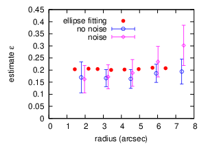
To test the ellipticity as a function of radius, we perform our method on stacked galaxy-galaxy lensing since the number density of background galaxies is not sufficient to study an individual galaxy. In each mock data projection, we use 10 flexion at random locations in an area of $20\times 20$ arcsec² (which is equal to 90 background galaxies/arcmin²). The data from 20 different projections are aligned and stacked with repect to the centre of the lens halo. 50 realisations are generated to calculate the mean value. Similar filters as in the last section are employed here, except that we discard data closer than 1 arcsec o the halo centre, or further than 8 arcsec away. The ellipticity using the surface mass density is calculated, and the average ellipticity over 20 projections is shown by the filled circles in Fig. 2. The open (blue) circles are the estimates from the flexion ratio method using data without intrinsic noise and the diamonds (purple) are those using noisy data. They are both averages over 50 realisations. The error bars represent the standard deviations in each bin. The error bars using noise free data in Fig. 2 are caused by the variances of halo ellipticities projected from different directions, while the error bars using noisy data are affected by the estimate error. We can see that the error bars increase with radius, as intrinsic noise becomes more important.

Refer to caption — Figure 1: Comparison of different halo ellipticity estimators using an NFW halo. The filled circles are estimated directly from fitting with surface mass ellipse, the crosses are estimated from the flexion ratio method (Sec. 3.2) with noise-free grid-based data. The diamonds are estimated using the clean method but with noisy data, and they are mean result over 50 realisations, the errors represent the standard deviations.

3.3 A cluster-sized halo

In addition, we test our approach on an $N$ -body simulated galaxy cluster halo. For galaxy clusters, we have more background galaxies in “observations”. Therefore the flexion number density is high enough to resolve an individual cluster. The test cluster halo PH-A-2 is taken from the PHOENIX simulations (Gao et al. 2011 in prep). At the second resolution level, the simulation has a softening length of $0.32h^{-1}$ kpc, mass resolution $5\times 10^{6}M_{\odot}h^{-1}$ . The main halo contains $1.5\times 10^{8}$ particles, with a total mass of $6.6\times 10^{14}M_{\odot}h^{-1}$ within a virial radius of $1.4h^{-1}$ Mpc. Two simulated cluster haloes are used to generate mock data: one has only the main halo, while the other one in addition includes massive subhaloes that are likely to have noticeable signatures. The number of subhaloes is about $5\%$ of the total subhaloes with mass $M>10^{9}M_{\odot}$ that are identified from the simulations. The halo is located at $z_{d}=0.5$ , while the background sources are chosen to be at $z_{s}=1.0$ . We project the same halo along 3 different directions to generate mock data.

In Fig. 3, the surface mass density $\kappa$ map from one projection (for the right panel in Fig. 4) is shown. One can see that there are some small scale fluctuations due to substructure. Moreover, the shape of the halo is not perfectly elliptical. It is easy to see that there is a bump on the left side of the halo. Both of these will cause some difficulties in estimating the halo ellipticity since flexion is sensitive to small scale variations. In each direction, we have 2 sets of data generated from the cluster haloes with and without subhaloes. We have 50 realisations with each having 800 background flexion data points on an area of $200\times 200$ arcsec². Such a configuration is available via the current surveys, e.g. the COSMOS survey has a background density of 76 galaxies/arcmin² (Schrabback et al., 2010). Similar filters as in previous sections with $\theta_{\rm min}=10$ arcsec and $\theta_{\rm max}=70$ arcsec are applied here. About 300 data points are obtained on average in each realisation. We make 6 bins in each realisation, and estimate the mean ellipticity and its standard deviation in each bin over the 50 realisations. The results are shown in Fig. 4. The filled circles are directly estimated from the surface mass density without substructure. The diamonds are the results from the data with the main halo, and the crosses are the results from the data with the main halo and the substructures. We can see that our estimates are slightly biased. The large error in the middle panel is caused by the intrinsic noise, which has very small ellipticity. In an additional test, we perform our estimates with a background galaxy number density of $45$ galaxies/arcmin² and obtain a similar result but with slightly larger errorbars ( $\sim 10\%$ ).

There are however some other reasons that can cause bias in our estimate. First of all, we need to point out that the estimate directly from mass is not the “true value” of the ellipticity. When we fit the iso-density contours using $\kappa$ , we notice that the orientations of different annuli are not aligned. Moreover, the annuli are not concentric, especially for clusters. Although our estimate using the flexion ratio does not depend on the radius or orientations, the binning of the data will be affected by the rapid variation of ellipticity and orientation. Secondly, the intrinsic noise and substructures will usually cause an overestimate (ES11). As pointed out by Bacon et al. (2010), the galaxy-galaxy lensing flexion varies due to substructures. As an additional test, we calculate the standard deviations of tangential flexion in each bin for our NFW halo and the PHOENIX halo with substructures. In Fig. 5, the values indicated by pluses are significantly smaller than the others since the NFW halo has regular shape and contains no substructures. The others from the PHOENIX halo have higher deviation as we expect. We can also see that the ellipticity also affects the deviations.

The centres of galaxy clusters are often not well determined from observations, e.g. it is often assumed that the mass centroid coincides with the brightest cluster galaxy, which may not be correct in all cases. Also mass and light peaks are often offset in the weak lensing shear method (Dietrich et al., 2011). On the other hand, in ES11 it has been found that a centroid offset to the true mass centre of the halo causes a slight overestimate of the halo ellipticity. The reason is that the flexion ratio is defined with respect to the true centre of halo mass, a centroid offset will introduce extra asymmetry in the estimate. Therefore, one can use the flexion ratio as a probe for the cluster centre, since $\langle r\rangle$ , $\langle r^{2}_{\rm obs}\rangle$ or an estimate of ellipticity, in principle, will reach its minimum when the flexion ratio is calculated with respect to the true mass centre. However the intrinsic and other kind of noises can cause some complications. In order to see this, we perform another test for the centroid offset problem. We generate 10 realisations of mock data. For each realisation, we use 100 random mock centres within 20 arcsec to the true mass centre. The flexion ratio and $\langle r^{2}_{\rm obs}\rangle$ are calculated with respect to the mock centre, and the result is shown in Fig. 6. One can see that although $\langle r^{2}_{\rm obs}\rangle$ does not reach minimum at the true centre of the cluster, the variance of $\langle r^{2}_{\rm obs}\rangle$ monotonically increases with the offset. This is also because, as we mentioned in the last paragraph, the mass distribution of galaxy clusters is complicated, e.g. the mass centre may vary with the radius. Nevertheless, the minimum flexion ratio statistics provides a complementary approach for cluster centre determination.

4 Conclusions and Discussions

In this paper, we have studied the flexion ratio method for estimating shapes of elliptical dark matter haloes. We performed numerical simulations to study our ellipticity estimators and obtained the halo ellipticity as a function of radius. In particular, for galactic-sized haloes, we are able to measure the mean variation of ellipticity with radius by stacking several galaxy samples. For cluster haloes, we can estimate the ellipticity as a function of radius for an individual galaxy cluster. We also point out that the minimum $\langle r^{2}_{\rm obs}\rangle$ provides another approach for determining the centre of galaxy clusters. Moreover, we introduced a weight function (in Appendix) to suppress the bias due to the asymmetric distribution of background galaxies. The variance of our estimate becomes significantly smaller after employing the weight function. We derived the second order statistics of the flexion ratio $\langle r^{2}\rangle$ and its analytical relation to $\langle r\rangle$ . By combining $\langle r\rangle$ and $\langle r^{2}\rangle$ , in principle the bias due to intrinsic noise can be subtracted. We provided a method to reduce the bias based on a linear approximation (For more details, see Eq. 25).

We however notice that there are some difficulties in estimating the halo ellipticity.

•

First of all, the noise model that we employ in this paper includes only intrinsic noise and numerical noise in the simulations. In reality there are other sources of noise, e.g. noises due to the point spread function and pixelisation. Moreover, the noise of flexion measurement appears different using different methods (Goldberg & Leonard, 2007). Thus the noise in practice may be non-Gaussian. Therefore, the results presented here are based on somewhat idealised observations.
•

The difficulty in reducing bias for small ellipticity haloes is mainly due to the lack of knowledge for the flexion noise behaviours. Moreover, the linear approximation that we employed is based on the assumption that the bias is independent of the halo ellipticity and is smaller than the flexion ratio signal. In reality, neither of these assumptions may be valid. In particular, for small elliptical haloes, our measurement will be dominated by intrinsic and other noises.
•

The optimal binning to the data is also difficult since we do not know how the ellipticity changes with radius. A coarse binning can only estimate the “mean” ellipticity. Moreover, as we show in the figures, flexion data on different radii have different signal-to-noise ratio (S/N), thus better data at small radii may be polluted by the low S/N data at large radii. On the other hand, if many bins are used, not enough galaxies will be contained within each bin.
•

The degeneracy of substructures and halo ellipticity: substructures behave similarly to intrinsic flexion in our estimate, but at different magnitudes. Substructures are therefore another kind of “noise”. On the other hand, flexion can be used to measure substructures in galaxies or clusters (e.g. their mass function and spatial distribution). Fig. 5 is a rough estimate by comparing the $\sigma_{F}$ magnitude without any knowledge of substructures or ellipticity. We can see that the combination of different approaches may constrain both shapes and substructures in dark matter haloes. Again good knowledge of flexion noise will be necessary. Also, a realistic model of the substructure mass function, and the spatial distribution of substructure will be helpful.

A high number density of background galaxies is desirable. Current surveys such as COSMOS may have sufficiently high galaxy number densities to enable our method to constrain mass ellipticities on a few radial bins for an individual galaxy cluster. This is again based on a simple noise model. In reality, the noise of high magnitude images is larger. The number density of high quality images using current observations may not as high as we used. For galaxy-sized haloes, we can perform stacking galaxy-galaxy lensing. Notice that different from the shear method, we do not need to align the major axis of the foreground galaxies. We do, however, assume that we can select dark matter haloes with similar shapes by carefully choosing the foreground galaxies according to their luminosity, colour and shape. The different morphologies will cause uncertainty in our estimate. On the other hand, the number density of galaxy-galaxy pairs will be very large in current and future surveys, i.e. the number of stacked galaxies in reality can be much higher than what we used in our test. Fig.2 indicates we can measure $\epsilon$ to standard deviation $\sigma_{\epsilon}\approx 0.05$ by stacking 20 foreground galaxies for $\epsilon\approx 0.2$ . With a much larger number of galaxies available in future observations, the accuracy of this measurement can be improved. The improvement will be Poissonian if there are no other sources of systematic errors. An accurate measurement of how the ellipticity varies with radius will provide a strong test of galaxy formation models.

Acknowledgments

We would like to thank Richard Long, Yougang Wang, Lin Yan and an anonymous referee for useful comments on the manuscript. We also thank Liang Gao for help on the PHOENIX simulation data.

Appendix A Bias estimate and reduction

In this appendix, we will introduce two approaches that will reduce the estimated error.

A.1 Weight function

One of the biases comes from the asymmetric distribution of background galaxies. To account for such effects, we introduce a weight function

w_{i}={1\over AN_{i}},

(16)

where $A$ is a normalisation, and $N_{i}$ is the number of background galaxies in a polar angle range $\Delta{\phi}$ centred at the $i$ th data. Therefore, the data is down-weighted where the number density is high. One can see that if the galaxy images are circularly symmetrically distributed with respect to the foreground lens galaxy/cluster, the weight function will be uniform $w_{i}=1/N$ , where $N$ is the total number of background galaxies. The weight function is employed when calculating the expectation flexion ratio from data

	$\displaystyle\bar{r}$	$\displaystyle=$	$\displaystyle\sum_{i=1}^{N}r_{i}w_{i};$		(17)
	$\displaystyle\bar{r^{2}}$	$\displaystyle=$	$\displaystyle\sum_{i=1}^{N}r^{2}_{i}w_{i}.$		(18)

A.2 Bias reduction

Due to the difficulty of measurement and our incomplete understanding of the point spread function (PSF), our knowledge about the intrinsic flexion is not sufficient to give an accurate noise model. Since flexion has a dimension of inverse length, the intrinsic flexion depends on the image size, and therefore the depth of survey. Moreover, Goldberg & Leonard (2007) found that different methods of measurement may lead to different noise behaviors.

In ES11, it has been found that estimates using flexion ratios will be larger than the true ones due to the intrinsic noise. Here we adopt a simple model for the bias in the flexion ratio $r$ , by assuming that the bias is independent of the halo ellipticity and lens strength. The observed mean flexion ratio can be written as

\langle r_{\rm obs}\rangle=\langle r\rangle+b_{r},

(19)

where $b_{r}$ stands for the bias in the $\langle r\rangle$ estimate. Notice that $b_{r}$ is not zero because the noise of the flexion ratio is not Gaussian (even if we assume that the noise of two flexion components is Gaussian, the ratio of two Gaussians no longer follows a Gaussian distribution). $\langle r^{2}\rangle$ can be obtained through two ways. First, we can directly calculate $\langle r^{2}_{\rm obs}\rangle$ from data using Eq.(18). Secondly, according to Eqs.(6) and (8), we have

\langle r^{2}_{\rm cal}\rangle={({\rm e}^{\pi\langle r\rangle/2}-1)^{2}\over 2{\rm e}^{\pi\langle r\rangle/2}}.

(20)

We can thus calculate $\langle r^{2}_{\rm cal}\rangle$ using Eq.(20) from $\langle r_{\rm obs}\rangle$ . The bias strength will be different in these two methods (Fig. 8). One can see that both estimates give larger values than the theoretical prediction (solid line), and they are different from each other. We make a first order expansion

$\displaystyle\langle r^{2}_{\rm obs}\rangle$	$\displaystyle=$	$\displaystyle\langle r^{2}\rangle+2\langle r\rangle b_{r}+O(b_{r}^{2});$	(21)
$\displaystyle\langle r^{2}_{\rm cal}\rangle$	$\displaystyle=$	$\displaystyle\langle r^{2}\rangle+{\partial\langle r^{2}\rangle\over\partial\langle r\rangle}b_{r}+O(b_{r}^{2})$	(22)
	$\displaystyle\approx$	$\displaystyle\langle r^{2}\rangle+{\pi\over 4}\left({\rm e}^{\pi\langle r\rangle/2}-{\rm e}^{-\pi\langle r\rangle/2}\right)b_{r}.$	(23)

The difference between $\langle r^{2}_{\rm obs}\rangle$ and $\langle r^{2}_{\rm cal}\rangle$ provides an estimate of the bias $b_{r}$ ,

	$\displaystyle\Delta$	$\displaystyle=$	$\displaystyle\langle r^{2}_{\rm obs}\rangle-\langle r^{2}_{\rm cal}\rangle$		(24)
		$\displaystyle\approx$	$\displaystyle\left(2\langle r\rangle-{\pi\over 4}\left({\rm e}^{\pi\langle r\rangle/2}-{\rm e}^{-\pi\langle r\rangle/2}\right)\right)b_{r}+O(b_{r}^{2}).$		(25)

We can subtract $b_{r}$ from the estimate, and obtain a relatively clean result. However, this only works for large $\epsilon$ . For small $\epsilon$ ( $\lesssim 0.1$ ), our approximation is no longer valid, since our measurements are dominated by noise. In the case of small $\epsilon$ , the $b_{r}^{2}$ term is larger than the other terms in Eq.(23), and thus cannot be neglected. Due to incomplete knowledge of the flexion noise, it is difficult to estimate when we should take the $b_{r}^{2}$ term into consideration. In practice, we first calculate $\langle r_{\rm obs}\rangle$ and $\langle r^{2}_{\rm obs}\rangle$ from the data, and then calculate $\langle r^{2}_{\rm cal}\rangle$ using Eq.(20). The bias is estimated through

b_{r}=\dfrac{\langle r^{2}_{\rm obs}\rangle-\langle r^{2}_{\rm cal}\rangle}{2\langle r_{\rm obs}\rangle-{\pi\over 4}\left({\rm e}^{\pi\langle r_{\rm obs}\rangle/2}-{\rm e}^{-\pi\langle r_{\rm obs}\rangle/2}\right)}.

(26)

If a negative $b_{r}$ is obtained, we use $b_{r}=2|\langle r^{2}_{\rm obs}\rangle-\langle r^{2}_{\rm cal}\rangle|$ as an empirical approximation.

Appendix B Numerical test with a non-singular isothermal ellipsoid model

In this section we describe some simulations that we have performed in order to test the behaviours of the estimators given in the previous section. We model the halo surface mass density by a non-singular isothermal ellipsoid (NIE) profile:

\kappa(\theta)={\theta_{\rm E}\over 2\sqrt{\theta_{c}^{2}+\theta^{2}}},

(27)

where the Einstein radius is $\theta_{\rm E}=6$ arcsec and the core radius is taken to be $\theta_{c}=2$ arcsec. The redshifts of mock sources are infinite. We have 50 flexion data points in each realisation, which are randomly distributed on $1\times 1$ arcmin² “source plane”. Data inside 6 arcsec and outside 30 arcsec are discarded (see Sect.3.1).

B.1 Test of the weight function

We generate 20 sets of mock data with different ellipticities $\epsilon=0.03i$ , $i=1,2,...20$ . For each ellipticity, we use 50 realisations. For each realisation, we calculate the expected flexion ratio in two ways. First, we calculate it directly using the mean of the data; second, we calculate $\langle r\rangle$ through our weight function (Eq.17). Then we estimate $\epsilon$ using Eq.(9). In Fig. 7, we show the mean estimate $\hat{\epsilon}$ over 50 realisations vs. the input values. The solid line shows the equality line, the pluses and circles are estimates with and without the weight function respectively. The error bars show the standard deviations. Both estimates closely trace the input values, but the ones with weight function have smaller variances, especially for large ellipticities. The bottom panel shows the relative error $|\delta\epsilon/\epsilon|$ . One can see that the biases with the weight function are significantly smaller, and all are below $2\%$ . Hence throughout this paper the weight function has been employed.

B.2 The bias reduction

We apply a simple model to generate noise in the data, ${\cal F}^{\rm obs}={\cal F}_{1}+n_{f1}+{\rm i}({\cal F}_{2}+n_{f2})$ (as in ES11). The intrinsic flexion noises $n_{f1},n_{f2}$ are drawn from a Gaussian distribution independently, each component is characterized by a standard deviation $\sigma_{{\cal F}1}=\sigma_{{\cal F}2}=0.03$ arcsec^-1.

We first compare $\langle r^{2}\rangle$ using two methods. In Fig. 8, we show $\langle r^{2}_{\rm obs}\rangle$ (pluses) and $\langle r^{2}_{\rm cal}\rangle$ (circles) of different input $\epsilon$ . For each $\epsilon$ , we plot 5 realisations. The solid line is the theoretical prediction. Although the noise is generated independent of $\epsilon$ , the error and difference between $\langle r^{2}_{\rm obs}\rangle$ and $\langle r^{2}_{\rm cal}\rangle$ do increase with $\epsilon$ .

Next we perform a test on our approach to bias reduction. 50 noise realisations for each $\epsilon$ are generated. In each realisation, $\langle r_{\rm obs}\rangle$ and $\langle r^{2}_{\rm obs}\rangle$ are calculated directly from the mock data, and $\langle r^{2}_{\rm cal}\rangle$ are calculated using Eq. (20). In Fig. 9 we compare the estimated values with the input ones (solid line). The pluses are the average of 50 realisations using Eq.(9). We also estimate the bias $b_{r}$ using Eq.(25), and obtain an estimate from $\langle r^{2}_{\rm clean}\rangle$ using Eq.(10). We need to point out that for small $\epsilon$ (in case of our noise model, $\epsilon$ $<0.1$ ), we adopt a modified approach since the linear approximation (Eq.25) is no longer valid. The results are shown by the circles in Fig. 9. Overall, the bias is reduced, but for small $\epsilon$ we still have larger errors. The bias reduction method is employed if not mentioned otherwise in Sect.3.

References

Allgood et al. (2006) Allgood B., Flores R. A., Primack J. R., Kravtsov A. V., Wechsler R. H., Faltenbacher A., Bullock J. S., 2006, MNRAS, 367, 1781
Bacon et al. (2010) Bacon D. J., Amara A., Read J. I., 2010, MNRAS, 409, 389
Bacon et al. (2006) Bacon D. J., Goldberg D. M., Rowe B. T. P., Taylor A. N., 2006, MNRAS, 365, 414
Bailin & Steinmetz (2005) Bailin J., Steinmetz M., 2005, ApJ, 627, 647
Bartelmann (1996) Bartelmann M., 1996, A&A, 313, 697
Bartelmann & Schneider (2001) Bartelmann M., Schneider P., 2001, Phys. Rep., 340, 291
Bett et al. (2010) Bett P., Eke V., Frenk C. S., Jenkins A., Okamoto T., 2010, MNRAS, 404, 1137
Bradač et al. (2008) Bradač M., Allen S. W., Treu T., Ebeling H., Massey R., Morris R. G., von der Linden A., Applegate D., 2008, ApJ, 687, 959
Bullock (2002) Bullock J. S., 2002, in P. Natarajan ed., The Shapes of Galaxies and their Dark Halos Shapes of Dark Matter Halos. pp 109–113
Cain et al. (2011) Cain B., Schechter P. L., Bautz M. W., 2011, arXiv:1103.0551
Clowe et al. (2006) Clowe D., Bradač M., Gonzalez A. H., Markevitch M., Randall S. W., Jones C., Zaritsky D., 2006, ApJ, 648, L109
Corless et al. (2009) Corless V. L., King L. J., Clowe D., 2009, MNRAS, 393, 1235
De Filippis et al. (2005) De Filippis E., Sereno M., Bautz M. W., Longo G., 2005, ApJ, 625, 108
Deb et al. (2010) Deb S., Goldberg D. M., Heymans C., Morandi A., 2010, ApJ, 721, 124
Debattista et al. (2008) Debattista V. P., Moore B., Quinn T., Kazantzidis S., Maas R., Mayer L., Read J., Stadel J., 2008, ApJ, 681, 1076
Dietrich et al. (2011) Dietrich J. P., Böhnert A., Lombardi M., Hilbert S., Hartlap J., 2011, ArXiv:1103.4607D
Dubinski & Carlberg (1991) Dubinski J., Carlberg R. G., 1991, ApJ, 378, 496
Er et al. (2010) Er X., Li G.L., Schneider P., 2010, arXiv:1008.3088
Er & Schneider (2011) Er X., Schneider P., 2011, A&A, 528, A52
Evans & Bridle (2009) Evans A. K. D., Bridle S., 2009, ApJ, 695, 1446
Faltenbacher et al. (2009) Faltenbacher A., Li C., White S. D. M., Jing Y., Mao S., Wang J., 2009, Research in Astronomy and Astrophysics, 9, 41
Fluke & Lasky (2011) Fluke C. J., Lasky P. D., 2011, arXiv: 1101.4407
Gao et al. (2011) Gao L. et al. 2011, in prep.
Goldberg & Bacon (2005) Goldberg D. M., Bacon D. J., 2005, ApJ, 619, 741
Goldberg & Leonard (2007) Goldberg D. M., Leonard A., 2007, ApJ, 660, 1003
Goldberg & Natarajan (2002) Goldberg D. M., Natarajan P., 2002, ApJ, 564, 65
Hawken & Bridle (2009) Hawken A. J., Bridle S. L., 2009, MNRAS, 400, 1132
Hilbert et al. (2011) Hilbert S., Gair J. R., King L. J., 2011, MNRAS, 412, 1023
Hoekstra et al. (2004) Hoekstra H., Yee H. K. C., Gladders M. D., 2004, ApJ, 606, 67
Howell & Brainerd (2010) Howell P. J., Brainerd T. G., 2010, MNRAS, pp 941
Irwin & Shmakova (2006) Irwin J., Shmakova M., 2006, ApJ, 645, 17
Jing & Suto (2002) Jing Y. P., Suto Y., 2002, ApJ, 574, 538
Kazantzidis et al. (2004) Kazantzidis S., Kravtsov A. V., Zentner A. R., Allgood B., Nagai D., Moore B., 2004, ApJ, 611, L73
Kuhlen et al. (2007) Kuhlen M., Diemand J., Madau P., 2007, ApJ, 671, 1135
Lee & Suto (2004) Lee J., Suto Y., 2004, ApJ, 601, 599
Leonard et al. (2007) Leonard A., Goldberg D. M., Haaga J. L., Massey R., 2007, ApJ, 666, 51
Leonard et al. (2009) Leonard A., King L. J., Wilkins S. M., 2009, MNRAS, 395, 1438
Mandelbaum et al. (2006) Mandelbaum R., Hirata C. M., Broderick T., Seljak U., Brinkmann J., 2006, MNRAS, 370, 1008
Massey et al. (2007) Massey R., Rowe B., Refregier A., Bacon D. J., Bergé J., 2007, MNRAS, 380, 229
Maulbetsch et al. (2007) Maulbetsch C., Avila-Reese V., Colín P., Gottlöber S., Khalatyan A., Steinmetz M., 2007, ApJ, 654, 53
Munshi et al. (2011) Munshi D., Smidt J., Heavens A., Coles P., Cooray A., 2011, MNRAS, pp 147
Munshi et al. (2008) Munshi D., Valageas P., van Waerbeke L., Heavens A., 2008, Phys. Rep., 462, 67
Natarajan & Refregier (2000) Natarajan P., Refregier A., 2000, ApJ, 538, L113
Navarro et al. (1996) Navarro J. F., Frenk C. S., White S. D. M., 1996, ApJ, 462, 563
Navarro et al. (1997) Navarro J. F., Frenk C. S., White S. D. M., 1997, ApJ, 490, 493
Oguri et al. (2010) Oguri M., Takada M., Okabe N., Smith G. P., 2010, MNRAS, 405, 2215
Okura et al. (2007) Okura Y., Umetsu K., Futamase T., 2007, ApJ, 660, 995
Okura et al. (2008) Okura Y., Umetsu K., Futamase T., 2008, ApJ, 680, 1
Ragone-Figueroa et al. (2010) Ragone-Figueroa C., Plionis M., Merchán M., Gottlöber S., Yepes G., 2010, MNRAS, 407, 581
Reblinsky (2000) Reblinsky K., 2000, A&A, 364, 377
Refregier (2003) Refregier A., 2003, ARA&A, 41, 645
Schaefer et al. (2011) Schaefer B. M., Heisenberg L., Fotios Kalovidouris A., Bacon D. J., 2011, arXiv: 1101.4769
Schneider & Er (2008) Schneider P., Er X., 2008, A&A, 485, 363
Schneider et al. (2006) Schneider P., Kochanek C. S., Wambsganss J., 2006, Gravitational Lensing: Strong, Weak and Micro
Schrabback et al. (2010) Schrabback T., Hartlap J., Joachimi B., Kilbinger M., Simon P., Benabed K., Bradač M., Eifler T., Erben T., Fassnacht C. D., High F. W., Hilbert S., Hildebrandt H., Hoekstra H., Kuijken K., Marshall P. J., Mellier Y., Morganson E., Schneider P., Semboloni E., van Waerbeke L., Velander M., 2010, A&A, 516, A63
Sereno et al. (2006) Sereno M., De Filippis E., Longo G., Bautz M. W., 2006, ApJ, 645, 170
Springel et al. (2008) Springel V., Wang J., Vogelsberger M., Ludlow A., Jenkins A., Helmi A., Navarro J. F., Frenk C. S., White S. D. M., 2008, MNRAS, 391, 1685
Springel et al. (2004) Springel V., White S. D. M., Hernquist L., 2004, in S. Ryder, D. Pisano, M. Walker, & K. Freeman ed., Dark Matter in Galaxies Vol. 220 of IAU Symposium, The shapes of simulated dark matter halos. pp 421
Suyu & Halkola (2010) Suyu S. H., Halkola A., 2010, A&A, 524, A94
van Haarlem & van de Weygaert (1993) van Haarlem M., van de Weygaert R., 1993, ApJ, 418, 544
Velander et al. (2010) Velander M., Kuijken K., Schrabback T., 2010, arXiv: 1011.3041
Vera-Ciro et al. (2011) Vera-Ciro C. A., Sales L. V., Helmi A., Frenk C. S., Navarro J. F., Springel V., Vogelsberger M., White S. D. M., 2011, ArXiv: 1104.1566
Wang et al. (2010) Wang H., Mo H. J., Jing Y. P., Yang X., Wang Y., 2010, ArXiv :1007.0612
Wang & Fan (2004) Wang Y., Fan Z., 2004, ApJ, 617, 847
Wang et al. (2010) Wang Y., Park C., Hwang H. S., Chen X., 2010, ApJ, 718, 762
Wang et al. (2008) Wang Y., Yang X., Mo H. J., Li C., van den Bosch F. C., Fan Z., Chen X., 2008, MNRAS, 385, 1511