The discovery of the family of charmonium and bottomonium resonances in the mid-1970s was greeted initially with simple descriptions in terms of non-relativistic $c\overline{c}$ and $b\overline{b}$ bound states, illustrating basic principles familiar from the earliest days of quantum mechanics [1, 2]. It has now come time to go beyond the simple $Q\overline{Q}$ picture of heavy quarkonium. Experiments have uncovered new degrees of freedom (many associated with flavored mesons) and are now at a level of accuracy sufficient to distinguish among many different schemes of relativistic corrections. We describe some of these recent developments in this brief review.

Scalar mesons below 1 GeV (Sec. 2) illustrate the importance of coupled channels and mesonic degrees of freedom. Another case in point, known for 50 years, is the $\Lambda(1405)$ (Sec. 3). The opening of new thresholds can lead to dips and cusps in mass spectra (Sec. 4); the interplay of closed and open channels is familiar from Feshbach resonances in nuclear physics.

Recent discoveries of $Q\overline{Q}q\overline{q}$ exotic states, where $Q,q$ denote heavy and light quarks, respectively, pose the question of whether these are genuine tetraquark states or more closely associated with states of a flavored meson $Q\overline{q}$ and antimeson $\overline{Q}q$. Exotic baryonium states were predicted 43 years ago (Sec. 5) but the jury is still out on their existence. One possibility for observing them is in $B$ meson decays. It appears that $Q\overline{Q}q\overline{q}$ states, probably in the form of $B\overline{B}^{*}$ and $B^{*}\overline{B}^{*}$ “molecules,” play a key role in the recent observation of the decays $\Upsilon(5S)\to\pi^{+}\pi^{-}h_{b}(1P,2P)$ (Sec. 6), through rescattering from states of open flavor.

We describe recent progress on radiative bottomonium transitions in Sec. 7, and conclude in Sec. 8.

A useful compendium of experimental references may be found in [3]. I draw heavily on the wisdom and common sense in two articles by D. Bugg [4, 5].

The following candidates for positive-parity spinless mesons (see Ref. [6] for a partial listing) probably owe their existence to the mesonic channels to which they couple:

• •

  $I=0$: The $\sigma(\sim 500)$, coupling to $\pi\pi$, is prominent in many Dalitz plots.

• •

  $I=1/2$: The $\kappa(\sim 750)$, coupling to $K\pi$, also appears frequently.

• •

  Another $I=0$ state, the $f_{0}(980)$, is closely correlated with the $K\overline{K}$ threshold.

• •

  The $I=1$ state $a_{0}(980)$ couples to $\eta\pi$ and $K\overline{K}$.

All the properties of the above mesons are closely linked to coupled channels. The $\sigma(500)$ is dynamically generated; it appears as a consequence of current algebra, crossing, unitarity, and assumption of a $\rho$ in the $I=J=1$ $\pi\pi$ channel [7]. One expects similar dynamics to generate a $\kappa$ in the $I=1/2$ $K\pi$ channel.

The $f_{0}(980)$ decays mainly to $\pi\pi$ but is produced largely from an $s\overline{s}$ initial state, e.g., in $B_{s}\to J/\psi s\overline{s}$. This behavior was noticed quite early in $J/\psi$ decays: The $f_{0}(980)$ appears in the $\pi\pi$ spectrum in $J/\psi\to\phi\pi\pi$ but not $J/\psi\to\omega\pi\pi$ [8].

A nonet structure (quark-diquark) has been proposed for the scalar mesons below 1 GeV [9]. However, it fails to describe quantitatively the couplings of these states to meson-meson channels [4].

The $\Lambda(1405)$ was originally identified 50 years ago as a low-energy $I=0$ S-wave $\Sigma$-$\pi$ resonance [10]. However, a key feature is its strong coupling to the $I=0$ S-wave $\overline{K}N$ channel, whose threshold lies $\sim 27$ MeV higher. The interaction between closed and open channels was studied extensively by Dalitz and Tuan in the late 1950s and early 1960s [11, 12, 13] and represents a realization of a Feshbach resonance, a phenomenon familiar from earlier instances of nuclear physics [14]. The opening of S-wave channels such as the $I=0$ $\overline{K}N$ channel coupling to $\Lambda(1405)$ can lead to cusps and dips in scattering amplitudes.

The $\Lambda(1405)$ fits the SU(6) $\otimes$ O(3) quark model as a $(70,~L=1~uds)$ state with $J^{P}=1/2^{-}$. Its large fine-structure splitting from the state $\Lambda(1520)$ with $J^{P}=3/2^{-}$ can be understood through interactions with final kaon-nucleon and pion-hyperon final states [15, 16]. More recently, the $\Lambda(1405)$ has been studied on the lattice [17] and recognized as a candidate for a $\overline{K}N$ molecule [18]. It thus can be viewed both as a conventional three-quark baryon and a meson-baryon composite. An analogous situation occurs for the $D_{s0}(2317)$, which can be viewed either as a ${}^{3}P_{0}$ $c\overline{s}$ state (lower in mass than expected), or as a $KD$ state with $~\sim 42$ MeV binding energy.

Rapid variations in mass spectra are ubiquitous near S-wave thresholds [4, 19, 20]. One sees cusps in the $M(\pi^{0}\pi^{0})$ spectrum from $K_{L}\to 3\pi^{0}$ decays at $\pi^{+}\pi^{-}$ threshold [21], permitting the measurement of the $\pi\pi$ S-wave scattering length difference $a_{0}-a_{2}$ [22]. Another cusp is visible in $M(\pi^{0}p)$ at $\pi^{+}n$ threshold [23].

If an elastic phase shift goes though $180^{\circ}$, the scattering amplitude vanishes: this is the Ramsauer–Townsend effect [24]. It leads to atomic or nuclear transparency at specific energies and can be utilized for making monochromatic neutron beams [25]. Sharp dips in mass spectra, often correlated with S-wave thresholds, occur in many instances of particle physics. One example is the S-wave $\pi\pi$ spectrum near $K\overline{K}$ threshold. The value of $R\equiv\sigma(e^{+}e^{-}\to{\rm hadrons})/\sigma(e^{+}e^{-}\to\mu^{+}\mu^{-})$ drops sharply around $\sqrt{s}=4.26$ GeV [26] (see Fig. 1), which happens to be just below the threshold for production of ($D\overline{D}_{1}~+$ charge conjugate), where $D$ and $D_{1}$ are charmed mesons with $J^{PC}=0^{-}$ and $1^{+}$, respectively. Diffractive photoproduction of $3\pi^{+}3\pi^{-}$ exhibits a dip near $p\overline{p}$ threshold [27, 28] (Fig. 2).

It has been suggested [29] that baryon-antibaryon states can form exotic ($qq\overline{q}\overline{q}$) mesons, as illustrated in Fig. 3. Indeed, if an ordinary meson contains a quark $q_{i}$ and another meson contains an antiquark $\overline{q}_{i}$ of the same flavor, they will form a resonance [Fig. 3(a)] when the center-of-mass (c.m.) 3-momentum typically does not exceed 350 MeV/$c$ [30]. The corresponding c.m. 3-momentum for formation of a meson-baryon resonance [Fig. 3(b)] is 250 MeV/$c$, and was estimated in Ref. [30] to be 200 MeV/$c$ for baryon-antibaryon resonance formation.

A flavor state which cannot be formed of $q_{1}\overline{q}_{2}$, such as $q_{1}q_{1}\overline{q}_{2}\overline{q}_{2}$ is truly exotic. $B$ meson decays offer numerous exotic final states, for example in $b\overline{d}\to c\overline{u}d\overline{d}$. Examples of suggestions for seeing exotics at $B$ factories [31, 32] are shown in Fig. 4.

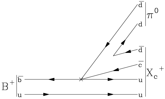
A bet was made with Peter Freund in 1972 that exotic baryonium would not be found in two years (he bet it would). He bought dinner in 1974; we are still waiting for the discovery. The decays of $B$ mesons can also yield pentaquarks ($qqqq\overline{q}$ candidates [31]); none have been seen so far.

Belle [33, 34] has reported a large cross section for $e^{+}e^{-}\to\pi^{+}\pi^{-}h_{b}(1P)$ or $\pi^{+}\pi^{-}h^{\prime}_{b}(2P)$ at the center-of-mass energy of $\Upsilon(5S)$. This is reminiscent of CLEO’s observation of a large cross section for $e^{+}e^{-}\to\pi^{+}\pi^{-}h_{c}$ at $\sqrt{s}=4170$ MeV [35, 36]. Earlier, BaBar [37, 38] and Belle [39] reported $\pi^{+}\pi^{-}$ and $\eta$ transitions to lower $\Upsilon$ states from $\Upsilon(4S)$ states; Belle [40] saw $\Gamma[\Upsilon(5S)\to\pi^{+}\pi^{-}\Upsilon(1S)]=(0.59\pm 0.04\pm 0.09)$ MeV, $\Gamma[\Upsilon(5S)\to\pi^{+}\pi^{-}\Upsilon(2S)]=(0.85\pm 0.07\pm 0.16)$ MeV, more than $10^{2}$ times the $nS$ rate for $n\leq 4$.

Some time ago Lipkin and Tuan [41] and Moxhay [42] pointed out that rescattering from $B^{(*)}\overline{B}^{(*)}$ would be important in quarkonium production from states above flavor threshold. More recent calculations [43, 44] support this point of view, borne out by the prominence of peaks in $\pi h_{b}$ mass spectra at $B\overline{B}^{*}$ and $B^{*}\overline{B}^{*}$ threshold reported at this Conference [34]. The masses of the $h_{b}(1P)$ and $h_{b}(2P)$ [33, 34], as well as the $h_{c}(1P)$ discovered earlier, are very close to the spin-weighted averages of the corresponding ${}^{3}P$ states, indicating small hyperfine splitting in $P$-wave mesons as expected in the naive quark model. Loop corrections from coupled channels largely cancel and are found to be insignificant [45].

One of many graphs contributing to the rescattering process $\Upsilon(5S)\to B\overline{B}^{*},B^{*}\overline{B}^{*},$ $\ldots\to\pi^{+}\pi^{-}h_{b}$ [5] is illustrated in Fig. 5. The energy must be above $B\overline{B}^{*}$ threshold in order to produce some $J^{P}(b\overline{b})$ values. A recent description by Bondar et al. [46] addresses selection rules whereby certain bottomonium states are favorably produced in rescattering. Rescattering through flavored pairs flips the $b\overline{b}$ spin from triplet to singlet in $\Upsilon(5S)\to\pi^{+}\pi^{-}h_{b}(1P,2P)$, whereas such a spin flip would be suppressed in perturbative QCD by an inverse power of the bottom quark mass.

The lowest-lying states of the bottomonium spectrum are illustrated in Fig. 6. We have heard about Belle’s conclusive observation of the $h_{b}(1P)$ and $h_{b}(2P)$ states [33, 34]. CLEO also searched for the $h_{b}(1P)$, via the transitions $\Upsilon(3S)\to(\pi^{+}\pi^{-}h_{b},~\pi^{0}h_{b},$
$h_{b}\to\gamma\eta_{b})$. A significant background to the $h_{b}$ search in the $\Upsilon(3S)\to\pi^{0}h_{b}$ decay [47] turned out to be the pairing of a photon from $\Upsilon(3S)\to\gamma\chi_{b}(1P)\to\gamma\gamma\Upsilon(1S)$, which required a more detailed study of these suppressed E1 transitions. This section describes that investigation [48].

Photons in the transitions $\Upsilon(3S)\to\gamma\chi_{b}(1P)$ and $\chi_{b}\to\gamma\Upsilon(1S)$ are in the 400–500 MeV range and can be a problematic background to the search for $\Upsilon(3S)\to\pi^{0}h_{b}$. The rates for $\Upsilon(3S)\to\gamma\chi_{b}(1P)$, while small, are poorly known. The electric dipole matrix element between 3S and 1P states vanishes for a harmonic oscillator potential and is highly suppressed for realistic quarkonium potentials [49]. Their values for various $\chi_{bJ}(1P)$ states thus test specific models of relativistic corrections, whose predictions span a wide range. Table 1 summarizes previously known branching fractions involving the $\chi_{bJ}(1P)$ states.

Heavy quarkonium theory now must confront light-quark degrees of freedom. Although we have been living with this since the dawn of hadron spectroscopy, new experimental results reinforce the viewpoint that mesonic degrees of freedom are important. Scalar mesons’ properties are governed by the $\pi\pi$, $K\pi$, and $K\overline{K}$ channels to which they couple. Effects of S-wave thresholds are ubiquitous.

We are still waiting for definitive evidence for tetraquark exotics. The recent discoveries by the Belle Collaboration of enhanced $h_{b}(1P)$ and $h_{b}(2P)$ production in $\Upsilon(5S)\to\pi^{+}\pi^{-}h_{b}(1P,2P)$ [33, 34] and of prominent enhancements of the $\pi h_{b}$ mass spectra at $B\overline{B}^{*}$ and $B^{*}\overline{B}^{*}$ thresholds [34] serve as a challenge to our understanding of hadron interactions, but indicate a key role for rescattering from flavored meson-antimeson intermediate states [5, 46].

Finally, progress in the study of bottomonium electromagnetic transitions has provided new data with which to confront models of relativstic corrections to naïve quarkonium pictures. We look forward to such calculations on a firmer footing.

ACKNOWLEDGEMENTS

This work was supported in part by the United States Department of Energy under Grant No. DE-FG02-90ER40560.

References

- [1] C. Quigg and J. L. Rosner, Phys. Rept. 56, 167 (1979).
- [2] H. Grosse and A. Martin, Phys. Rept. 60, 341 (1980).
- [3] N. Brambilla et al., Eur. Phys. J. C 71, 1534 (2011) [arXiv:1010.5827 [hep-ph]].
- [4] D. V. Bugg, presented at 10th International Workshop on Meson Production, Properties and Interaction (MESON 2008), Cracow, Poland, 6–10 Jun 2008, arXiv:0806.3566 [hep-ph].
- [5] D. V. Bugg, “Meson Spectroscopy without Tetraquarks,” arXiv:1101.1659 [hep-ph].
- [6] K. Nakamura et al. [Particle Data Group], J. Phys. G 37, 075021 (2010).
- [7] R. L. Goble, R. Rosenfeld and J. L. Rosner, Phys. Rev. D 39, 3264 (1989), and earlier references therein.
- [8] G. J. Feldman and M. L. Perl, Phys. Rept. 33, 285 (1977).
- [9] R. L. Jaffe, Phys. Rev. D 15, 267, 281 (1977).
- [10] M. H. Alston, L. W. Alvarez, P. Eberhard, M. L. Good, W. Graziano, H. K. Ticho and S. G. Wojcicki, Phys. Rev. Lett. 6, 698 (1961).
- [11] R. H. Dalitz and S. F. Tuan, Phys. Rev. Lett. 2, 425 (1959).
- [12] R. H. Dalitz and S. F. Tuan, Annals Phys. 8, 100 (1959)
- [13] R. H. Dalitz and S. F. Tuan, Annals Phys. 10, 307 (1960)
- [14] H. Feshbach, Ann. Phys. (N.Y.) 5, 357 (1958). See also U. Fano, Nuovo Cim. 12, 154 (1935) [Translation: J. Res. Natl. Inst. Stand. Technol. 110, 583 (2005)]; Phys. Rev. 124, 1866 (1961).
- [15] N. Isgur and G. Karl, Phys. Lett. B 72, 109 (1977).
- [16] N. Isgur and G. Karl, Phys. Rev. D 18, 4187 (1978).
- [17] M. Lage, U. G. Meissner and A. Rusetsky, Phys. Lett. B 681, 439 (2009) [arXiv:0905.0069 [hep-lat]].
- [18] T. Hyodo and D. Jido, arXiv:1104.4474 [nucl-th].
- [19] E. P. Wigner, Phys. Rev. 73, 1002 (1948).
- [20] J. L. Rosner, Phys. Rev. D 74, 076006 (2006) [arXiv:hep-ph/0608102].
- [21] J. R. Batley et al. [NA48/2 Collaboration], Phys. Lett. B 633, 173 (2006).
- [22] N. Cabibbo, Phys. Rev. Lett. 93, 121801 (2004); N. Cabibbo and G. Isidori, JHEP 0503, 021 (2005); G. Colangelo, J. Gasser, B. Kubis and A. Rusetsky, Phys. Lett. B 638, 187 (2006), and references therein.
- [23] A. Schmidt et al., Phys. Rev. Lett. 87, 232501 (2001).
- [24] C. Ramsauer, Ann. der Physik (Leipzig) Ser. 4, 64, 513 (1921); ibid. 66, 545 (1921) [see also H. F. Mayer, ibid. 64, 451 (1921)]; J. S. Townsend and V. A. Bailey, Phil. Mag. Ser. 6, 43, 593 (1922); ibid. 44, 1033 (1922); N. F. Mott and H. S. W. Massey, The Theory of Atomic Collisions, 3rd Ed., Ch. 18 (Oxford University Press, 1965). For a recent discussion see W. R. Johnson and C. Guet, Phys. Rev. A 49, 1041 (1994).
- [25] P. S. Barbeau, J. I. Collar and P. M. Whaley, Nucl. Instrum. Meth. A 574, 385 (2007) [arXiv:nucl-ex/0701011].
- [26] J. Z. Bai et al. [BES Collaboration], Phys. Rev. Lett. 88, 101802 (2002).
- [27] P. L. Frabetti et al. [E687 Collaboration], Phys. Lett. B 514, 240 (2001).
- [28] P. L. Frabetti et al., Phys. Lett. B 578, 290 (2004).
- [29] J. L. Rosner, Phys. Rev. Lett. 21, 950 (1968).
- [30] J. L. Rosner, Phys. Rev. D 6, 2717 (1972).
- [31] J. L. Rosner, Phys. Rev. D 69, 094014 (2004) [arXiv:hep-ph/0312269].
- [32] K. Terasaki, arXiv:1102.3750 [hep-ph].
- [33] I. Adachi et al. [Belle Collaboration], arXiv:1103.3419 [hep-ex].
- [34] A. Bondar, this Conference.
- [35] T. K. Pedlar et al. [CLEO Collaboration], Cornell University Report CLNS 11/2073, arXiv:1104.2025 [hep-ex], submitted to Phys. Rev. Letters.
- [36] J. L. Rosner, “Charm at Threshold,” this Conference.
- [37] B. Aubert et al. [BABAR Collaboration], Phys. Rev. Lett. 96, 232001 (2006) [arXiv:hep-ex/0604031].
- [38] B. Aubert et al. [BABAR Collaboration], Phys. Rev. D 78, 112002 (2008) [arXiv:0807.2014 [hep-ex]].
- [39] A. Sokolov et al. [Belle Collaboration], Phys. Rev. D 75, 071103 (2007) [arXiv:hep-ex/0611026].
- [40] K. F. Chen et al. [Belle Collaboration], Phys. Rev. Lett. 100, 112001 (2008) [arXiv:0710.2577 [hep-ex]].
- [41] H. J. Lipkin and S. F. Tuan, Phys. Lett. B 206, 349 (1988).
- [42] P. Moxhay, Phys. Rev. D 39, 3497 (1989).
- [43] C. Meng and K. T. Chao, Phys. Rev. D 77, 074003 (2008) [arXiv:0712.3595 [hep-ph]]; C. Meng and K. T. Chao, Phys. Rev. D 78, 034022 (2008) [arXiv:0805.0143 [hep-ph]]; C. Meng and K. T. Chao, Phys. Rev. D 78, 074001 (2008) [arXiv:0806.3259 [hep-ph]].
- [44] Yu. A. Simonov and A. I. Veselov, Phys. Lett. B 671, 55 (2009) [arXiv:0805.4499 [hep-ph]]; Yu. A. Simonov and A. I. Veselov, Phys. Lett. B 673, 211 (2009) [arXiv:0810.0366 [hep-ph]].
- [45] T. J. Burns, arXiv:1105.2533 [hep-ph].
- [46] A. E. Bondar, A. Garmash, A. I. Milstein, R. Mizuk and M. B. Voloshin, arXiv:1105.4473 [hep-ph].
- [47] J. Y. Ge et al. [CLEO Collaboration], arXiv:1106.3558 [hep-ex].
- [48] M. Kornicer et al. [CLEO Collaboration], Phys. Rev. D 83, 054003 (2011) [arXiv:1012.0589 [hep-ex]].
- [49] A. K. Grant, J. L. Rosner, A. Martin, J. M. Richard and J. Stubbe, Phys. Rev. D 53, 2742 (1996) [arXiv:hep-ph/9506315].
- [50] U. Heintz et al., Phys. Rev. D 46, 1928 (1992).
- [51] T. Skwarnicki (CLEO Collaboration), in Proceedings of the 31st International Conference on High Energy Physics (ICHEP 2002), Amsterdam, The Netherlands, 24-31 Jul 2002, Elsevier, Amsterdam, 2003, Parallel Sessions: ISBN 0 444 51343 4, pp. 698-702.
- [52] J. P. Lees et al. [BABAR Collaboration], arXiv:1104.5254 [hep-ex].
- [53] M. Artuso et al. (CLEO Collaboration), Phys. Rev. Lett. 94, 032001 (2005).
- [54] P. Moxhay and J. L. Rosner, Phys. Rev. D 28, 1132 (1983); S. N. Gupta, S. F. Radford, and W. W. Repko, Phys. Rev. D 30, 2424 (1984); H. Grotch, D. A. Owen, and K. J. Sebastian, Phys. Rev. D 30, 1924 (1984); F. Daghighian and D. Silverman, Phys. Rev. D 36, 3401 (1987); J. P. Fulcher, Phys. Rev. D 42, 2337 (1990); T. A. Lähde, Nucl. Phys. A 714, 183 (2003); D. Ebert, R. N. Faustov, and V. O. Galkin, Phys. Rev. D 67, 014027 (2003).
- [55] W. Kwong and J. L. Rosner, Phys. Rev. D 38, 279 (1988).
- [56] W. Kwong. P. Mackenzie, R. Rosenfeld, and J. L. Rosner, Phys. Rev. D 38, 3210 (1988).
- [57] S. Bethke, Eur. Phys. J. C 64, 689 (2009) [arXiv:0908.1135 [hep-ph]].