Orbit-Based Dynamical Models of the Sombrero Galaxy (NGC 4594)Note: Accepted to ApJ: 30 June 2011
Abstract
We present axisymmetric, orbit-based models to study the central black hole, stellar mass-to-light ratio, and dark matter halo of NGC 4594 (M104, the Sombrero Galaxy). For stellar kinematics, we use published high-resolution kinematics of the central region taken with the Hubble Space Telescope, newly obtained Gemini long-slit spectra of the major axis, and integral field kinematics from the SAURON instrument. At large radii, we use globular cluster kinematics to trace the mass profile and apply extra leverage to recovering the dark matter halo parameters. We find a black hole of mass , and determine the stellar (uncertainties are the 68% confidence band marginalized over the other parameters). Our best fit dark matter halo is a cored logarithmic model with asymptotic circular speed and core radius kpc. The fraction of dark to total mass contained within the half-light radius is . Taking the bulge and disk components into account in our calculation of puts NGC 4594 squarely on the - relation. We also determine that NGC 4594 lies directly on the - relation.
Subject headings
galaxies: individual (M104, NGC 4594)—galaxies: kinematics and dynamics—galaxies: photometryI. Introduction
Most galaxies are thought to host supermassive black holes (SMBHs) at their centers. The masses of these SMBHs have been observed to correlate with several properties of their host elliptical galaxies and of the classical bulge components of their host disk galaxies. For example, correlates with galaxy/bulge mass [12, 45, 41, 49, 48, 26], luminosity (the - relation) [30, 38, 35, 25], velocity dispersion (the - relation) [17, 21, 68, 25], and globular cluster content [7, 27]. These and other, similar correlations suggest that galaxy formation and black hole growth are fundamentally linked. To better understand this interplay, accurate black hole masses are needed.
One challenge that limits the accuracy is the determination of the host galaxy’s inclination. Projection effects are difficult to model and cause loss of information, leading to systematic uncertainties. Therefore, SMBHs in galaxies whose inclination is confidently known have the best chance of being accurately and robustly measured. Another issue that limits the accuracy is the effect a dark matter halo has on the determination of SMBH mass. Gebhardt & Thomas [19] show that orbit-based models can underestimate black hole mass when dark matter is not considered in the modeling, however Schulze & Gebhardt [57] find the effect is small when the black hole’s sphere of influence is well-resolved.
NGC 4594 (M104, or the Sombrero Galaxy) is a nearly edge-on Sa type spiral with a prominent stellar disk and large, classical bulge [37]. The shape of this disk indicates that it (and thus the entire galaxy) is inclined at an angle very close to . Throughout this paper we assume a distance to NGC 4594 of 9.8 Mpc, calculated from surface brightness fluctuations [67]. Unless otherwise stated, all distance-dependent quantities are scaled to this value. Tonry et al. [67] use a value of in their distance determinations, however we compare our and to Gültekin et al. [25] who adopt in their work. We therefore scale the Gültekin et al. [25] distances down by . Black hole mass scales as and luminosity as ; these quantities are adjusted accordingly.
NGC 4594 was one of the first galaxies in which a black hole was detected, and it has a long history of study. Kormendy(1988, hereafter 29) first found evidence for a massive black hole of using only ground-based observations. With isotropic Jeans models, Emsellem et al. [15] measured a black hole of mass . Later, Kormendy et al. (1996, hereafter 40) used high-resolution kinematics from the Faint Object Spectrograph (FOS) on the Hubble Space Telescope (HST)—the same data set we include—to measure . This corresponds to a mass of . With isotropic models, Magorrian et al. [45] obtained a value of . These values for all lie towards the high mass end of the - and - relations. Massive SMBH measurements are frequently being revised, and we expect the confidently known inclination of NGC 4594 to lead to one of the more secure measurements of a high mass SMBH.
We present new Gemini spectroscopy of the major axis, as well as SAURON integral field kinematics covering the central region of the galaxy. We also use high-resolution HST/FOS kinematics of the nucleus and kinematics derived from globular clusters at large radii. We combine these kinematic datasets with HST and ground-based photometry to run axisymmetric orbit-based models. These models allow us to measure the black hole mass, stellar mass-to-light ratio, and dark matter halo of NGC 4594. In addition, we also recover information about the internal orbit structure of the galaxy.
II. Data Reduction and Analysis
Dynamical modeling requires as input the three-dimensional luminosity density distribution , as well as the line-of-sight velocity distribution (LOSVD) at many locations in the galaxy. We use HST and ground-based images for the photometry. Our kinematics include high-resolution HST/FOS spectra, long-slit spectra from GNIRS on Gemini, SAURON integral field kinematics, and individual velocities of globular clusters (GCs). We discuss each in turn.
II.1. Photometry
In order to cover a large enough dynamical range to have leverage on both the central SMBH and dark halo, we use surface brightness profiles from HST and ground-based images. The stellar disk of NGC 4594 dominates at intermediate radii on the major axis causing the isophotes in this region to be substantially flattened. This abrupt change in ellipticity introduces an additional challenge to the deprojection. Our standard technique is to assume that the surfaces of constant luminosity density are coaxial, similar spheroids [20]. Clearly the presence of a disk invalidates this assumption, so we decompose the surface brightness into bulge and disk components, deprojecting each separately so that our assumption holds for each component. Afterwards, we re-combine the deprojected profile of each component and input the total into our modeling program.
The bulge-disk decomposition fits directly to a projected image. We construct a model disk by considering a Sérsic [59] profile:
| (1) |
where is the surface brightness at and is the Sérsic index. For , the profile is an exponential. For inclinations other than , the projection of our disk model is an ellipse. By specifying the inclination of the disk , the axial ratio of the ellipse is given by for a thin disk.
We construct many disk models by varying , , , and (keeping close to 1). Each model is then subtracted from the image until the residual brightness distribution has elliptical isophotes. The remaining light is assigned to the bulge component. A 1D major axis bulge profile is produced by averaging the bulge light in elliptical, annular isophotes. Hence, we are left with an analytic disk model and a non-parametric bulge model. We identify the best bulge and disk models as those that minimize the rms residuals of the model-subtracted image.
| Disk | (mag arcsec-2) | (arcsec) | ||
|---|---|---|---|---|
| Outer 1 | 18.8 | 66.8 | 1.0 | 80 |
| Outer 2 | 16.7 | 40.1 | 1.0 | 80 |
| Nuclear | 20.4 | 4.1 | 1.1 | 83 |
In addition to the obvious main disk, NGC 4594 hosts a well-studied nuclear disk (Burkhead 8,29,40) at small radii. We fit the nuclear disk in the HST image and the main disk in the ground-based image. Because we fit directly to the images, dust lanes and object masking become important. We keep a bad pixel list which instructs our code to ignore trouble spots. Dust lanes are selected by eye, while SExtractor [3] is used to identify foreground stars, background galaxies, and globular clusters.
II.1.1 HST Image
To probe the nuclear region, we use a PSF-deconvolved HST Wide Field Planetary Camera 2 (WFPC2) image (GO-5512; PI: Faber). This image is presented in 40 and provides an excellent view of the central region of the galaxy. Centered on the PC1 camera, the image is taken in the F547M filter, and has a scale of 00455 pixel-1 of the central of the galaxy. The PSF deconvolution uses the Lucy-Richardson algorithm [53, 43] for 40 iterations and is well-tested on WFPC2 images [42]. The best fit parameters from the bulge-disk decomposition are listed in Table 1.
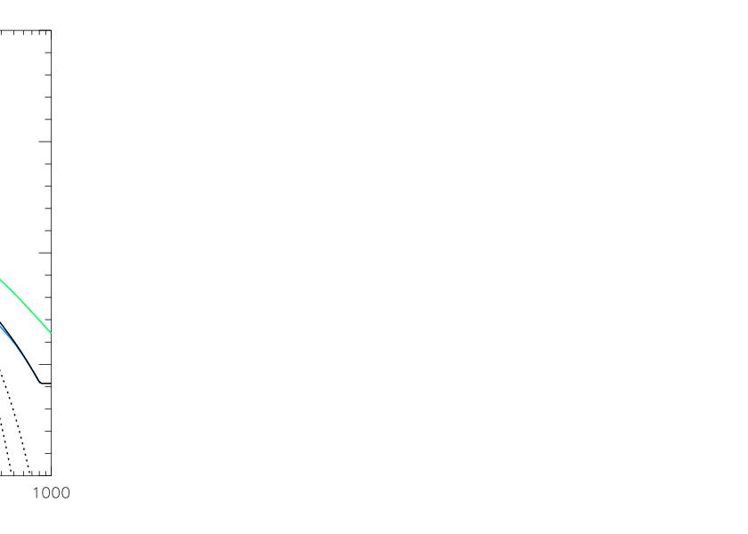
NGC 4594 is also thought to have weak LINER emission [2] and there is a point source in the HST image. Furthermore, heavy dust absorption also makes the determination of the central bulge surface brightness profile difficult for . To deal with these issues, we extrapolate the bulge surface brightness inwards to with a constant slope fit to the region near . Figure 1 shows the result of this extrapolation, as well as the other components fit in the ground-based image.
II.1.2 Ground-Based Image
We obtained a wide-field, -band image from the Prime Focus Camera on the McDonald 0.8 m telescope. This instrument provides a large unvignetted field of view (4545 arcmin2 ) and a single CCD detector. Therefore, we can more robustly carry out sky-subtraction and accurately constrain the faint isophotes. The image is corrected for bias, flat field, and illumination using standard routines in IRAF.
In our fit to the ground-based image, we ignore the central due to over-exposure and contamination from the nuclear disk. We attempt fits in the region with only one stellar disk given by Equation (1), however these produce unacceptable residuals. Instead of modifying Equation (1), we add a second disk (in addition to the nuclear disk fit only in the HST image). This approach is similar to the Multi-Gaussian Expansion technique used to model the light distribution of bulges and ellipticals [14]. A summary of all components fit is given in Table 1 and plotted in Figure 1.
II.1.3 Globular Cluster Profile
Globular clusters (GCs) are essentially bright test particles that allow us to probe the potential at radii where the stellar light is faint. They have been used in orbit-based models of other galaxies [19, 60, 50]. To include them in our models, we use the GC number density profile [52] as an analog to the stellar density. The number density profile is converted to a surface brightness profile by arbitrarily adjusting the zero point to match the stellar profile in log space.
The green line in Figure 1 shows that the slope of the GC surface brightness profile is different from that of the stars. We run models using both the measured luminosity density distribution of the GCs and assuming that of the stars. We find significant preference for the measured GC profile.
II.1.4 Bulge Profile
Our bulge-disk decomposition returns a non-parametric form of the bulge profile. It is not necessary to have a parameterized bulge profile for our dynamical models, however we fit a Sérsic profile to ground-based bulge model using Equation (1). The bulge is well-fit by a Sérsic function, with the rms residuals equal to . We measure ,, and .
We can convert the central surface brightness and radius parameters to the more familiar “effective” parameters and . The effective radius is given by and the effective surface brightness [44]. The factor depends on ; an expansion for can be found in MacArthur et al. [44]. Applying these conversions, we obtain and .
We obtain a simpler estimate for the half-light radius of the bulge from integration of the surface brightness profile; no fitting functions are required. We estimate . The integrated magnitudes are calculated for component by . This does not take into account the ellipticity of each component, so we scale the luminosity by where is the ellipticity of each component, assumed to be constant with radius. The bulge profile is known to become rapidly circular for [8] so our procedure almost certainly underestimates and . These numbers are computed as a sanity check only, and do not affect the dynamical models.
The absolute integrated magnitudes are and in F814W, corrected for Galactic extinction along the line of sight [56]. Using the HST calibration package SYNPHOT (described in detail below), we convert these F814W magnitudes to -band Vega magnitudes. We obtain and . These structural parameters lie exactly on the fundamental plane for bulges and ellipticals as presented in Kormendy et al. [32]. Our integrated magnitudes translate to a bulge-to-total ratio with the nuclear disk contributing of the total light. This value of is lower than previous measurements—Kormendy et al. [31] report . Our , however, is in good agreement with a recent measurement by Gadotti [18, model BD]. Regardless of the value of , our dynamical models are unaffected, because we add all the bulge and disk light together again after the deprojection.
We do not explore the possibility of fitting an exponential stellar halo in addition to a bulge and disk as Gadotti [18] do. Our bulge-disk decomposition produces a non-parametric bulge profile which could in principle be a combination of a Sérsic bulge plus exponential halo. However, this resulting profile is well-fit by a Sérsic function with significantly larger than 1. We therefore do not agree with the claim made by Gadotti [18] that the bulge of NGC 4594 is actually an exponential stellar halo.
II.1.5 Deprojection
We combine the HST and ground-based bulge profiles by zero-pointing both to F814W. We calculate the F547M photometric zero point for the HST image from the SYNPHOT package in IRAF. Spectral template fitting (Section II.2.1) shows that in the central region of the galaxy of the light comes from K6III stars. We therefore convert the F547M zero point to F814W with SYNPHOT using the Bruzual Atlas11 1 http://www.stsci.edu/hst/observatory/cdbs/bz77.html template for a K6III star.
Before deprojection, we extrapolate the one-dimensional profiles with a constant slope to . The three disk profiles are then combined and deprojected via Abel inversion in the manner described in Gebhardt et al. [20]. We assume an inclination of . The inclinations of the combined disk components imply an ellipticity of . Our composite bulge profile is deprojected in a similar fashion, assuming a constant ellipticity of 0.25 [8]. We then add to obtain the total luminosity density distribution input to our models.

The globular cluster luminosity density profile is obtained via a similar deprojection, but with the additional assumption of spherical symmetry. The normalization of the GC light profile is irrelevant, as our models fit only to the slope of the profile.
II.2. Kinematics
Kinematics for NGC 4594 come from four sources. The first uses near-IR data from Gemini/GNIRS long-slit observations along the major axis. These data were taken under good seeing conditions (around 05) and has high . The second set comes from the Faint Object Spectrograph (FOS) on HST using the square aperture of and is published in 40. The third set of data is from the SAURON instrument [16]. The SAURON data for NGC 4594 have not been published previously. Individual velocities from globular clusters are our fourth source of kinematics. These data are published in Bridges et al. [6]. We describe each dataset in detail.
II.2.1 Gemini Kinematics
We use GNIRS [13] on the Gemini South Telescope to measure near-IR spectra of NGC 4594. The data were taken on 17 January, 2005. We placed the 150″030 slit along the major axis with the galaxy nucleus centered within the slit. We use a spatial pixel size of 015. With the 32l l/mm grating in 3rd order, we obtain a wavelength coverage of 19800–26200 Å at 6.4 Å per pixel. Using sky lines, we measure a resolving power around 1700 or an instrumental dispersion of 75 km s-1. The total on-target exposure is 24 minutes, taken in 12, 2-minute individual exposures. Sky frames of equal exposure are taken throughout.
From both setup images and images of telluric standards, we measure a FWHM in the spatial direction of 05, assuming a Gaussian distribution. We use this PSF for the dynamical models.
We use a custom pipeline to reduce the GNIRS data; however, it produces very similar results to the Gemini GNIRS reduction package. The pipeline includes dark subtraction, wavelength calibration for the individual exposures, sky subtraction, registration and summing.
There is adequate signal to extract kinematics out to a radius of 45″. Figure 2 shows an example spectrum, where we plot the data in black and the template convolved with the best-fit line-of-sight velocity distribution (LOSVD). The velocity templates come from the GNIRS spectral library [73], where we select stars with a range of types from G dwarf to late giant. The kinematic extraction program performs a simultaneous fit to the LOSVD and relative weights of the templates. This procedure is described in Gebhardt et al. [21] and Pinkney et al. [51]. We present these data in the form of Gauss-Hermite moments in Table 2.
II.2.2 HST/FOS Kinematics
40 present HST/FOS kinematics of the nuclear region of NGC 4594. The FOS has a aperture. There are three pointings with accurately known positions for NGC 4594 (GO-5512; PI: Faber). The dynamical models include the exact placement and aperture size for the FOS pointing [40], and use the HST PSF [21].
| arcsec | ||||||||
|---|---|---|---|---|---|---|---|---|
| 0.00 | 19 | 14 | 253 | 16 | -0.087 | 0.033 | 0.023 | 0.046 |
| 0.15 | -36 | 11 | 257 | 12 | -0.008 | 0.042 | -0.016 | 0.038 |
| 0.30 | -75 | 12 | 249 | 8 | -0.053 | 0.048 | -0.017 | 0.037 |
| 0.52 | -112 | 11 | 234 | 8 | 0.020 | 0.037 | -0.047 | 0.035 |
| 0.82 | -144 | 12 | 221 | 9 | 0.060 | 0.038 | -0.051 | 0.032 |
| 1.20 | -172 | 9 | 202 | 9 | 0.065 | 0.039 | 0.003 | 0.031 |
| 1.73 | -190 | 8 | 185 | 9 | 0.107 | 0.031 | 0.018 | 0.031 |
| 2.40 | -208 | 7 | 184 | 9 | 0.089 | 0.032 | 0.024 | 0.031 |
| 3.30 | -232 | 8 | 175 | 9 | 0.140 | 0.029 | 0.044 | 0.027 |
| 4.57 | -236 | 9 | 171 | 7 | 0.173 | 0.032 | 0.023 | 0.027 |
| 6.45 | -235 | 7 | 178 | 9 | 0.165 | 0.033 | 0.058 | 0.025 |
| 8.77 | -189 | 11 | 203 | 11 | 0.028 | 0.039 | -0.007 | 0.036 |
| 11.40 | -171 | 10 | 192 | 10 | 0.071 | 0.033 | -0.009 | 0.033 |
| 14.32 | -187 | 16 | 185 | 15 | 0.227 | 0.042 | 0.102 | 0.060 |
| 17.70 | -201 | 13 | 229 | 16 | -0.023 | 0.042 | 0.020 | 0.050 |
| 22.20 | -228 | 12 | 198 | 14 | 0.125 | 0.040 | 0.052 | 0.047 |
| 28.58 | -235 | 11 | 194 | 14 | 0.122 | 0.042 | 0.036 | 0.051 |
| 36.08 | -285 | 6 | 141 | 10 | 0.046 | 0.041 | 0.032 | 0.034 |
| 44.40 | -277 | 7 | 149 | 9 | 0.094 | 0.042 | 0.101 | 0.039 |
| -0.15 | 45 | 12 | 240 | 15 | -0.026 | 0.034 | 0.002 | 0.041 |
| -0.30 | 112 | 11 | 243 | 15 | -0.052 | 0.036 | -0.016 | 0.038 |
| -0.52 | 130 | 10 | 224 | 15 | -0.080 | 0.043 | 0.014 | 0.037 |
| -0.82 | 162 | 8 | 212 | 10 | -0.068 | 0.049 | 0.019 | 0.030 |
| -1.20 | 176 | 7 | 206 | 11 | -0.066 | 0.047 | 0.065 | 0.031 |
| -1.73 | 205 | 7 | 190 | 12 | -0.087 | 0.043 | 0.022 | 0.037 |
| -2.40 | 226 | 7 | 173 | 12 | -0.101 | 0.037 | 0.053 | 0.039 |
| -3.30 | 244 | 9 | 187 | 11 | -0.113 | 0.039 | 0.037 | 0.037 |
| -4.65 | 246 | 8 | 184 | 12 | -0.130 | 0.035 | 0.025 | 0.040 |
| -6.15 | 237 | 9 | 220 | 14 | -0.133 | 0.042 | 0.094 | 0.035 |
| -8.40 | 221 | 9 | 211 | 13 | -0.191 | 0.051 | 0.079 | 0.036 |
| -10.95 | 162 | 9 | 209 | 14 | -0.093 | 0.048 | 0.028 | 0.043 |
| -14.25 | 178 | 9 | 198 | 14 | -0.092 | 0.059 | 0.046 | 0.042 |
| -19.20 | 204 | 10 | 198 | 17 | -0.166 | 0.060 | 0.094 | 0.048 |
| -24.52 | 207 | 11 | 193 | 17 | -0.045 | 0.057 | 0.029 | 0.052 |
| -29.33 | 241 | 11 | 182 | 16 | -0.149 | 0.054 | 0.092 | 0.050 |
| -36.15 | 271 | 11 | 180 | 12 | -0.084 | 0.046 | 0.053 | 0.042 |
| -45.15 | 274 | 10 | 141 | 9 | -0.053 | 0.041 | -0.029 | 0.028 |
Note. — Kinematics along the major axis of NGC 4594. Gauss-Hermite moments were derived from the LOSVDs that are the input to the dynamical models.
II.2.3 SAURON Kinematics
We also include SAURON integral field kinematics The SAURON data are from a single pointing exposing on the central region, taken in the low resolution setting of the instrument [1]. In addition to and , the SAURON data also include the higher order Gauss-Hermite moments and . Details of the data reduction and analysis can be found in Bacon et al. [1], Emsellem et al. [16].
Our modeling code fits to the entire LOSVD rather than its moments, so we reconstruct LOSVDs from the Gauss-Hermite moments. We create 100 Monte Carlo realizations of a non-parametric LOSVD from the uncertainties in the Gauss-Hermite parameters of each SAURON bin [19]. The 1433 reconstructed SAURON LOSVDs are spatially sampled more finely than our modeling bins. We therefore average the SAURON data to match our binning by weighting according to the uncertainties in the LOSVDs.
We re-construct Gauss-Hermite moments from the combined SAURON LOSVDs for plotting purposes only. Figure 3 shows these moments near the major and minor axes. The major axis for the SAURON data is significantly lower than that measured for the Gemini data. The reason for this is that SAURON data are binned to match the gridding of our model bins. Near the major axis, the bins range in polar angle from . These bins are described by a single LOSVD constructed by averaging individual LOSVDs which sample the region at smaller spatial scales. Thus, the average LOSVD contains contributions from LOSVDs as much as above the major axis.
II.2.4 Globular Cluster Kinematics
At large radii, we use individual globular cluster velocities published in Bridges et al. [6] to derive LOSVDs. The data contain positions and radial velocities for 108 globular clusters in NGC 4594. We discard the innermost 14 GCs as there are too few GCs inside to reconstruct an LOSVD in the inner parts of the galaxy. Assuming axisymmetry, the positions of the GCs are folded about the minor and major axes. In order to preserve rotation, we flip the sign of the velocity for all GCs that are folded about the minor axis. The GCs are then divided into annular bins extending from to at radii of , , , , and with roughly 20 GCs per bin.
Within each spatial bin, we calculate the LOSVD from the discrete GC velocities by using an adaptive kernel density estimate adapted from Silverman [61] and explained in Gebhardt et al. [20]. Each LOSVD contains 15 velocity bins. The velocity bins are highly correlated for the GCs, and there are likely only a few degrees of freedom per LOSVD. The - uncertainties in the LOSVDs are estimated through bootstrap resamplings of the data [20, 19].
We compute Gauss-Hermite moments from the GC LOSVDs—again for plotting purposes only—and show these in Figure 3. Uncertainties are calculated by fitting moments to each resampling of the LOSVD during the bootstrap. The GC kinematics resemble the minor axis stellar kinematics in many of the panels. For example, their dispersions appear to be an extrapolation of the minor axis velocity dispersions. There is slight rotation (small ) and possible evidence of radial anisotropy (positive ).

III. Dynamical Models
The dynamical models rely on the orbit superposition technique first developed by Schwarzschild [58]. We assume axisymmetry and match the luminosity density profile and kinematics of the galaxy to those reconstructed from an orbit library. The library is populated with orbits carefully chosen to sample E, , and the third, non-classical integral .
The code used in this paper is described in Gebhardt et al. [21], Gebhardt et al. [22], Thomas et al. [66], Thomas et al. [64], and Siopis et al. [62]. Similar axisymmetric codes are presented in Rix et al. [54], van der Marel et al. [72], Cretton et al. [11], and Valluri et al. [70]. Van den Bosch et al. (2008) present a fully triaxial Schwarzschild code. The basic outline of our code is as follows: (i.) convert the luminosity density distribution into the stellar density via an assumed stellar mass-to-light ratio . (ii.) Add to this density the contribution from a black hole of mass and a dark matter halo with density profile . (iii.) Calculate the potential associated with this density distribution and integrate a large number of orbits (typically 20,000) over many dynamical times. (iv.) Assign a weight to each orbit and determine the values by minimizing the difference between the observed kinematics and luminosity density of the galaxy and those resulting from the PSF-convolved orbit library, subject also to the constraint of maximum entropy.
We maximize the entropy-like quantity where is the Boltzmann entropy and controls the relative weight of or . For small values of , reproducing the observed kinematics becomes unimportant, and the models act to only maximize entropy. As increases, maximizing entropy becomes less important, and more weight is given to matching the observations. In practice, we start with a small value of and gradually increase it until asymptotes. The interested reader may see Siopis et al. [62] or Shen & Gebhardt [60] for more details.
Our model grid consists of 19 radial and 5 azimuthal bins covering a radial range of 003 to 1800″spaced logarithmically. Additionally, we use 15 velocity bins to describe our LOSVDs. We incorporate the effects of seeing by convolving the light distribution for each orbit with a model PSF before comparing with data [21]. We approximate the PSF as Gaussian with a FWHM of either , or depending on whether the data are from SAURON, Gemini, or HST observations respectively. The convolution extends to a radius of .
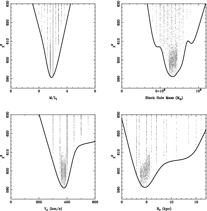
We run over 8,500 models with different values of the model parameters , , and . We use statistics to determine the best fit parameter values and their uncertainties. Models whose values of are within of the minimum for a given model parameter (marginalized over the others) define the - or 68% confidence band of that parameter.
III.1. Model Assumptions
Our fiducial density profile is a combination of stellar mass, dark matter, and a central SMBH:
| (2) |
where is the stellar mass-to-light ratio, assumed constant with radius and is the Dirac delta function. The angle is the angle above the major axis. While can in principle be a function of , we do not consider flattened models. We assume a spherically symmetric, logarithmic halo of the form:
| (3) |
This profile is cored for radii and produces a flat rotation curve with circular speed for . It has two free parameters, and , which are varied in the fitting process. Including and , this brings the total number of model parameters to four.
Recently, Gebhardt & Thomas [19] have shown that the inclusion of a dark matter halo can significantly affect modeled BH masses. To test for this, we run a smaller suite of models without a dark halo.
IV. Results
Our best-fit values for the four model parameters are , , , and kpc. Figure 4 shows the minima around each of the model parameters. Each dot represents a single model and the solid curve is a smoothed fit to the minimum. The points of the solid curve at above the minimum determine the - confidence limits on the parameters. All four model parameters have well-behaved curves with sharp, well-defined minima. This allows robust determination of the model parameters with small - uncertainties.

The uncertainties we present are derived strictly from statistics. The - error bars on quoted parameters correspond to models within of the minimum value. Systematic effects are likely to contribute in addition to this quoted uncertainty. While in general for other galaxies one of the biggest sources of systematic uncertainty is inclination, for NGC 4594 inclination uncertainties are unimportant. Other sources of uncertainty may include effects due to non-axisymmetries, but these are likely small or zero since only the most massive ellipticals are thought to be significantly triaxial [4, 36, 69]. For more on systematic uncertainties, the reader is referred to Gebhardt et al. [22] and Gültekin et al. [24], Gültekin et al. [25].
Figure 5 shows correlations among the four model parameters. Plotted are the different projections of the four dimensional parameter space; every small dot corresponds to a model run. Red dots are models that lie within of the minimum, and large black dots are within . There appears to be a slight correlation between and —much less severe than in M87 [19]. Not surprisingly, the high resolution of our HST kinematics is able to break the degeneracy between and . We discuss this further below. The dark halo parameters do not show any obvious correlation, indicating the GC and stellar kinematics were able to break the degeneracy usually observed between these two parameters.
Our best fit model has (unreduced) . It is non-trivial to calculate the number of degrees of freedom . Roughly, , however there are complicated correlations between velocity bins [22]. With this crude estimate for , our best fit model has reduced .
We compare the modeled value of our stellar mass-to-light ratio with that obtained from evolutionary population synthesis models [46, 47]. We adopt values of 10 Gyr and 0.1 for the stellar age and metallicity of NGC 4594 [55] and use these to derive the predicted I-band from the Maraston models. For a Salpeter IMF with stellar masses drawn from the range , this analysis yields . If instead the stars obey a Kroupa IMF drawn from the same range, then . We multiply these by a factor of 1.096 corresponding to to correct for Galactic extinction along the line of sight [56] to obtain and . Our dynamically-derived stellar falls nicely between these two values.
In Figure 6, we plot the total mass-to-light ratio as a function of radius for our best fit model with - uncertainties (gray region). The red cross-hatched region represents the range in stellar from stellar population models described above. Total rises near the center of the galaxy due to the contribution of the supermassive black hole. As we go out in radius, the stars become more important to the total mass over roughly the range to . Here the total approaches both our dynamically determined and the range derived from stellar population models. Past once again rises due to the importance of the dark halo.
Figure 7 plots the enclosed mass of each component as well as the total mass of the galaxy. At our innermost bin, the total mass is almost two orders of magnitude greater than the stellar mass, meaning we are probing the black hole’s sphere of influence quite well. The green line plotted is the mass profile Kormendy & Westpfahl [39] derive from their gas rotation curve. It agrees well with the total mass distribution derived here.

IV.1. Models without Dark Matter
We run 189 models with no dark halo. In these models, we exclude the globular cluster data and use only the stellar kinematics. Correspondingly, the number of degrees of freedom impacting the unreduced are proportionately fewer. We measure a black hole mass of and stellar mass-to-light ratio of . The minimum unreduced , proving models without a dark halo are a worse fit.
We do not see the dramatic change that Gebhardt & Thomas [19] see in M87 where the inclusion of a DM halo causes their determination of to double. Instead, our results mirror those of Shen & Gebhardt [60] in NGC 4649 where the inclusion of a DM halo does not significantly change the modeled . The likely explanation for this behavior is the inclusion of high resolution HST kinematics in both NGC 4649 and NGC 4594. Schulze & Gebhardt [57] find the same effect for a larger sample of galaxies. Whenever the data have high enough resolution to resolve the black hole’s radius of influence , dark matter has no significant effect on the determination of . For NGC 4594 we measure . We use HST/FOS kinematics whose central pointing has a PSF of . Additionally, the light profile of NGC 4594 is more centrally concentrated than that of M87. These factors combine to allow a more accurate determination of , removing the freedom that the models have to trade mass between and . This is evidenced by the lack of correlation among and in Figure 5.

IV.2. Orbit Structure
Having already determined the orbital weights that provide the best fit to the data, we reconstruct the internal unprojected moments of the distribution function. We perform this analysis on our best fit model and the models that define the 68% confidence region (over all combinations of the four model parameters), yielding internal moments at each grid cell.
We define the tangential velocity dispersion to be where is actually the second moment, containing contributions from both streaming and random motion in the direction. Figure 8 shows the radial run of the ratio . The second moment of the DF is tangentially biased where the disk is important (gray region) as expected but mostly is isotropic elsewhere. The red region plots for stars near the minor axis, showing almost perfect isotropy. The green region indicates that at large radii, globular cluster kinematics show significant radial anisotropy. We discuss the implications of this in Section V.2 below.

V. Discussion
V.1. Black Hole-Bulge Correlations
We discuss the position of NGC 4594 on the - and - relations, as defined by Gültekin et al. (2009b, hereafter 25) and compare our values of the correlation parameters to previous measurements. We calculate the effective velocity dispersion similar to 25
| (4) |
where is the rotational velocity and is the surface brightness profile. This makes essentially the surface-brightness-weighted second moment. Instead of integrating from the center of the galaxy () as 25 did, we integrate from to ensure that we do not bias with the high dispersion near the black hole. Our outermost kinematic data point is at , thus we have a gap in kinematic coverage between . The velocity dispersion near the end of our long-slit data is dropping sharply, however may still contribute to the integral for . To investigate this, we use the gas rotation curve presented in Kormendy & Westpfahl [39] which extends well beyond . Truncating the integral at gives while using the extended rotation curve yields .
The problem with this definition of is that it includes a contribution from the rotation of the disk. It has been shown that black hole mass does not correlate with disk properties [31] so this is not ideal. However, to compare with 25 we must be consistent in our calculation of . We therefore quote this value of when we compare to the - relation determined by 25. As we expect black hole mass to track bulge quantities, disk contribution to is likely to add a source of intrinsic scatter to spiral galaxies in the - relation. In fact, spiral galaxies are observed to have larger scatter about - than ellipticals of similar .
We also discuss some possible alternatives to where we attempt to remove the disk contribution. One option is to remove from Equation (4) altogether. Bulges are known to rotate, however, [36] and this will likely underestimate . This crude calculation gives .
Another option is to assume some degree of bulge rotation a priori. If we assume NGC 4594 rotates isotropically [36], then its flattening determines its position on the diagram [4]. Kormendy [28] shows that the relation
| (5) |
approximates the isotropic rotator line to roughly accuracy. We use our value of the bulge ellipticity in Equation (5) and assume this value of applies globally to the entire bulge. We then use our measured dispersion profile to determine the bulge velocity . Using these quantities, we determine . We compare this to the kinematics listed in Kormendy & Illingworth [36]. These data include long-slit spectra taken at a position angle parallel to the major axis, but , , and above it. From these data, it is apparent that the bulge off the major axis is roughly constant at . The rotation velocity rises from 0 to at large radii. We estimate the luminosity-weighted mean . Adding this in quadrature to the constant bulge gives . This estimate does not contain any rotation from the disk, and is consistent with our determination of obtained by assuming a constant .


Our black hole mass agrees nicely with that of 25 which uses the 29 value. In fact, when corrected for their various distance determinations, most values of in the literature agree quite well (29, Emsellem et al. 15, 40, Magorrian et al. 45) despite the many modeling techniques and datasets used. This is likely due to the high degree of isotropy as evidenced in Figure 8, deduced from the diagram [36], and noted in 29.
Figure 9 plots the position of NGC 4594 on the 25 - and - relations. We plot each determination of in the left-hand panel. Straightforward application of Equation (5) leads to a value of that falls directly on the 25 - line (blue asterisk). Next closest is the method of calculating by assuming a value of (green square). This point lies dex above the 25 line, however this is still within the estimated scatter. The calculation of that ignored all rotation is, not surprisingly, farthest from the 25 line. Calculation of the relevant quantities for comparison with the - relation is straightforward, and we plot our value of and (green square) along with that from 25 in the right-hand panel.
V.2. Globular Clusters
As demonstrated in section IV.2, we find significant radial anisotropy in the globular clusters. It is interesting that the stellar kinematics at smaller radii do not show this feature. This difference in orbital properties combined with the difference in their light profiles might suggest the GCs and stars are two distinct populations of tracer particles. This could also indicate the two populations have different formation scenarios.
Unfortunately, there is no radius in the galaxy where we have simultaneous coverage of both stellar and GC kinematics. Thus, we are unable to test whether the stellar orbits become more radial in the between where the stellar kinematics run out and the GCs begin. However, since the light profiles of both populations are significantly different (Figure 1) there is no reason to assume they should share similar orbit properties.
Figure 8 shows the globular clusters in NGC 4594 are radially anisotropic () over roughly the radial range - (approximately 1-10 ). Previous studies of the GC systems of galaxies have found their velocity ellipsoids to be isotropic [10, 9]. However, these studies used spherical Jeans modeling instead of the more general axisymmetric Schwarzschild code we use.
Rhode & Zepf [52] determine with high confidence that the color distribution of the GC system in NGC 4594 is bimodal. This may indicate different subpopulations of GCs with different orbital properties that formed at different epochs in the galaxy’s history. In our analysis, we make no distinction between red and blue subpopulations. We use the light profile and kinematics of all available GCs, regardless of color. However, since we use different sources for our kinematics and photometry data, there is the possibility that each source draws from a different GC subpopulation.
V.3. Dark Halo
The parameters and of our model dark halo imply a central dark matter density of Using an improved Jeans modeling technique, Tempel & Tenjes [63] model NGC 4594 and find a dark matter halo with central density , ten times lower than our value. They, however, measure a larger stellar in the bulge.
We plot the fraction of enclosed mass that is dark matter as a function of half-light radius in Figure 10. At there is already a roughly - mix of stars and DM. Inside of the dark matter still contributes a non-negligible fraction to the total mass content.
In a study measuring dark matter properties in local () early-type galaxies from the Sloan Digital Sky Survey, Grillo [23] find a correlation between the fraction of dark matter within and the logarithmic value of . With our measured value of , this correlation predicts a dark matter fraction at of . Our value of is smaller, but still within their 68% confidence limit.
Thomas et al. [65] derive scaling relations for halo parameters based on observations of early-type galaxies in the Coma cluster. These relations are constructed for similar galaxies using the same halo parameterization and modeling code used in this paper. This makes comparison to our parameters straightforward. We compare to the observed relations between halo parameters , , and and total blue luminosity . Our value of falls directly on the - relation, however our measured is smaller by roughly an order of magnitude. Since , the discrepancy in causes our measurement of to be high when compared to the Thomas et al. [65] - relation. Scatter in this relation is large, however, and the environment of NGC 4594 is different from that of the Coma galaxies.
Kormendy & Freeman [33], Kormendy & Freeman [34] also derive scaling laws for similar parameters in galaxies of later Hubble type (Sc-Im). We measure a much higher density and much smaller core radius than the Kormendy & Freeman [33], Kormendy & Freeman [34] relations imply at the of NGC 4594. We interpret this as the result of severe compression of the halo by the gravity of the baryons [5]. Such an effect is expected in early-type galaxies with massive bulges.
References
- [1] Bacon, R., et al. 2001, MNRAS, 326, 23
- [2] Bendo, G. J., et al. 2006, ApJ, 645, 134
- [3] Bertin, E., & Arnouts, S. 1996, A&AS, 117, 393
- [4] Binney, J. 1978, MNRAS, 183, 501
- [5] Blumenthal, G. R., Faber, S. M., Flores, R., & Primack, J. R. 1986, ApJ, 301, 27
- [6] Bridges, T. J., Rhode, K. L., Zepf, S. E., & Freeman, K. C. 2007, ApJ, 658, 980
- [7] Burkert, A., & Tremaine, S. 2010, ApJ, 720, 516
- [8] Burkhead, M. S. 1986, AJ, 91, 777
- [9] Côté, P., McLaughlin, D. E., Cohen, J. G., & Blakeslee, J. P. 2003, ApJ, 591, 850
- [10] Côté, P., et al. 2001, ApJ, 559, 828
- [11] Cretton, N., de Zeeuw, P. T., van der Marel, R. P., & Rix, H. 1999, ApJS, 124, 383
- [12] Dressler, A. 1989, in IAU Symposium, Vol. 134, Active Galactic Nuclei, ed. D. E. Osterbrock & J. S. Miller (Dordrecht: Kluwer), 217–+
- [13] Elias, J. H., Joyce, R. R., Liang, M., Muller, G. P., Hileman, E. A., & George, J. R. 2006, in Presented at the Society of Photo-Optical Instrumentation Engineers (SPIE) Conference, Vol. 6269, Society of Photo-Optical Instrumentation Engineers (SPIE) Conference Series
- [14] Emsellem, E., Monnet, G., & Bacon, R. 1994a, A&A, 285, 723
- [15] Emsellem, E., Monnet, G., Bacon, R., & Nieto, J. 1994b, A&A, 285, 739
- [16] Emsellem, E., et al. 2004, MNRAS, 352, 721
- [17] Ferrarese, L., & Merritt, D. 2000, ApJL, 539, L9
- [18] Gadotti, D. A. 2011, ArXiv e-prints
- [19] Gebhardt, K., & Thomas, J. 2009, ApJ, 700, 1690
- [20] Gebhardt, K., et al. 1996, AJ, 112, 105
- [21] —. 2000, ApJL, 539, L13
- [22] —. 2003, ApJ, 583, 92
- [23] Grillo, C. 2010, ApJ, 722, 779
- [24] Gültekin, K., et al. 2009a, ApJ, 695, 1577
- [25] —. 2009b, ApJ, 698, 198
- [26] Häring, N., & Rix, H. 2004, ApJL, 604, L89
- [27] Harris, G. L. H., & Harris, W. E. 2011, MNRAS, 410, 2347
- [28] Kormendy, J. 1982, in Saas-Fee Advanced Course 12: Morphology and Dynamics of Galaxies, ed. L. Martinet & M. Mayor (Sauverny: Observatoire de Genève), 113–288
- [29] Kormendy, J. 1988, ApJ, 335, 40
- [30] Kormendy, J. 1993, in The Nearest Active Galaxies, ed. J. Beckman, L. Colina, & H. Netzer (Madrid: Consejo Superior de Investigaciones Cientificas), 197–218
- [31] Kormendy, J., Bender, R., & Cornell, M. E. 2011, Nature, 469, 374
- [32] Kormendy, J., Fisher, D. B., Cornell, M. E., & Bender, R. 2009, ApJS, 182, 216
- [33] Kormendy, J., & Freeman, K. C. 2004, in IAU Symposium, Vol. 220, Dark Matter in Galaxies, ed. S. Ryder, D. Pisano, M. Walker, & K. Freeman (San Fransisco: ASP), 377–+
- [34] Kormendy, J., & Freeman, K. C. 2011, in preparation
- [35] Kormendy, J., & Gebhardt, K. 2001, in American Institute of Physics Conference Series, Vol. 586, 20th Texas Symposium on relativistic astrophysics, ed. J. C. Wheeler & H. Martel (San Fransisco: ASP), 363–381
- [36] Kormendy, J., & Illingworth, G. 1982, ApJ, 256, 460
- [37] Kormendy, J., & Kennicutt, Jr., R. C. 2004, ARA&A, 42, 603
- [38] Kormendy, J., & Richstone, D. 1995, ARA&A, 33, 581
- [39] Kormendy, J., & Westpfahl, D. J. 1989, ApJ, 338, 752
- [40] Kormendy, J., et al. 1996, ApJL, 473, L91+
- [41] Laor, A. 2001, ApJ, 553, 677
- [42] Lauer, T. R., Faber, S. M., Ajhar, E. A., Grillmair, C. J., & Scowen, P. A. 1998, AJ, 116, 2263
- [43] Lucy, L. B. 1974, AJ, 79, 745
- [44] MacArthur, L. A., Courteau, S., & Holtzman, J. A. 2003, ApJ, 582, 689
- [45] Magorrian, J., et al. 1998, AJ, 115, 2285
- [46] Maraston, C. 1998, MNRAS, 300, 872
- [47] —. 2005, MNRAS, 362, 799
- [48] Marconi, A., & Hunt, L. K. 2003, ApJL, 589, L21
- [49] McLure, R. J., & Dunlop, J. S. 2002, MNRAS, 331, 795
- [50] Murphy, J. D., Gebhardt, K., & Adams, J. J. 2011, ApJ, 729, 129
- [51] Pinkney, J., et al. 2003, ApJ, 596, 903
- [52] Rhode, K. L., & Zepf, S. E. 2004, AJ, 127, 302
- [53] Richardson, W. H. 1972, Journal of the Optical Society of America (1917-1983), 62, 55
- [54] Rix, H., de Zeeuw, P. T., Cretton, N., van der Marel, R. P., & Carollo, C. M. 1997, ApJ, 488, 702
- [55] Sánchez-Blázquez, P., Gorgas, J., Cardiel, N., & González, J. J. 2006, A&A, 457, 809
- [56] Schlegel, D. J., Finkbeiner, D. P., & Davis, M. 1998, ApJ, 500, 525
- [57] Schulze, A., & Gebhardt, K. 2011, ApJ, 729, 21
- [58] Schwarzschild, M. 1979, ApJ, 232, 236
- [59] Sérsic, J. L. 1968, Atlas de Galaxias Australes (Cordoba: Observatorio Astronomico, Univ. Cordoba)
- [60] Shen, J., & Gebhardt, K. 2010, ApJ, 711, 484
- [61] Silverman, B. W. 1986, Density estimation for statistics and data analysis (London: Chapman and Hall)
- [62] Siopis, C., et al. 2009, ApJ, 693, 946
- [63] Tempel, E., & Tenjes, P. 2006, MNRAS, 371, 1269
- [64] Thomas, J., Saglia, R. P., Bender, R., Thomas, D., Gebhardt, K., Magorrian, J., Corsini, E. M., & Wegner, G. 2005, MNRAS, 360, 1355
- [65] —. 2009, ApJ, 691, 770
- [66] Thomas, J., Saglia, R. P., Bender, R., Thomas, D., Gebhardt, K., Magorrian, J., & Richstone, D. 2004, MNRAS, 353, 391
- [67] Tonry, J. L., Dressler, A., Blakeslee, J. P., Ajhar, E. A., Fletcher, A. B., Luppino, G. A., Metzger, M. R., & Moore, C. B. 2001, ApJ, 546, 681
- [68] Tremaine, S., et al. 2002, ApJ, 574, 740
- [69] Tremblay, B., & Merritt, D. 1996, AJ, 111, 2243
- [70] Valluri, M., Merritt, D., & Emsellem, E. 2004, ApJ, 602, 66
- [71] van den Bosch, R. C. E., van de Ven, G., Verolme, E. K., Cappellari, M., & de Zeeuw, P. T. 2008, MNRAS, 385, 647
- [72] van der Marel, R. P., Cretton, N., de Zeeuw, P. T., & Rix, H. 1998, ApJ, 493, 613
- [73] Winge, C., Riffel, R. A., & Storchi-Bergmann, T. 2009, ApJS, 185, 186