,
Power-law forgetting in synapses with metaplasticity
Abstract
The idea of using metaplastic synapses to incorporate the separate storage of long- and short-term memories via an array of hidden states was put forward in the cascade model of Fusi et al. In this paper, we devise and investigate two models of a metaplastic synapse based on these general principles. The main difference between the two models lies in their available mechanisms of decay, when a contrarian event occurs after the build-up of a long-term memory. In one case, this leads to the conversion of the long-term memory to a short-term memory of the opposite kind, while in the other, a long-term memory of the opposite kind may be generated as a result. Appropriately enough, the response of both models to short-term events is not affected by this difference in architecture. On the contrary, the transient response of both models, after long-term memories have been created by the passage of sustained signals, is rather different. The asymptotic behaviour of both models is, however, characterised by power-law forgetting with the same universal exponent.
1 Introduction
Human memories are known to be fickle, but they are also capable of being elephantine. While research in this field is longstanding [1] in the field of psychology, it is only relatively recently that it has been attacked from an interdisciplinary perspective. The seminal work of Amit and collaborators [2, 3, 4] on neural networks was in large part responsible for opening up the field to physicists [5]; much the same can be said about the work of Hopfield [6]. The optimisation of learning on complex neuronal networks has been a field in itself; it has generally assumed that memories are stored via the abrupt change that occurs in the synapses connecting neurons, when they are exposed to a particular pattern. This picture is premised on the notion of binary synapses (‘synaptic switches’), which are a natural approximation to synapses possessing a finite set of discrete states. There is some experimental evidence [7, 8] in their support, and they have also been extensively used in earlier mathematical models (see e.g. [9, 10, 11]).
The above mechanism of synaptic plasticity has, however, been shown to be rather inefficient when synapses change permanently [12]. Pure plasticity indeed does not provide a mechanism for protecting some memories while leaving room for other, newer, memories to come in, hence the need for the mechanism of metaplasticity [3]. In order to improve performance, Fusi et al [13] proposed a cascade model of a synapse with many hidden states, which they claimed was able to store long-term memories more efficiently, with a decay that was power-law rather than exponential in time. Such power-law forgetting has in fact also been observed experimentally [14, 15] (albeit at a behavioural rather than a synaptic level). This issue forms the focus of the current paper, where we also put Fusi et al’s cascade model on a more quantitative basis, by submitting it to detailed questioning in a way that has not been done in either the original work or in subsequent papers. Another aim of our work is to see whether the introduction of architectural differences might induce important differences in behaviour: we accordingly devise a model which has a different mechanism for the decay of long-term memories, compared to the one of Fusi et al, and compare the two models.
The plan of this paper is as follows. In Section 2 we define both models to be investigated. Model I is an extension of the original cascade model by Fusi et al, whereas Model II has a different architecture. Both models however share the common feature that all the transition probabilities decay exponentially with the level depth of the hidden states. Section 3 presents the formalism of Markov chains used in this work. The default states of the two models are studied in Section 4. This allows us to identify some useful parameters, which include static and dynamical lengths and relevant to the problem. Section 5 is devoted to the response of both models to a single long-term potentiating (LTP) input signal and to a DC signal (sustained LTP signal); here we also provide an investigation of universal asymptotic power-law forgetting (common to both models) and of the non-universal transient forgetting specific to Model II. In Section 6 we study the signal-to-noise ratio which emerges from an investigation of fluctuations around the default state, while in Section 7 we illustrate the response of the models to a selection of specific time-dependent input signals. While some of these signals may be seen to be biologically unrealistic, they are necessary for a systematic study of our models, viewed from a physicist’s perspective as signal processing units. Finally, we discuss our results in Section 8. Appendix A contains a detailed investigation of the problem of the logarithmic walker, whereas Appendix B examines the transient behaviour of both models, and includes a derivation of the non-universal transient exponent of Model II.
2 The models
In this section, we define the models to be studied and introduce some of the ideas relevant to our investigations. Synapses can respond differently to an incoming action potential, in a way that could change with time [16]: if a particular stimulation paradigm leads to a persistent increase in response, this leads to the long-term potentiation of synapses (LTP), whereas long-term depression (LTD) corresponds to the opposite limit. This change in the strength of a synapse from a weak to a strong state and vice versa is referred to as synaptic plasticity and forms the basis of the current understanding of learning and memory, when applied to the many interconnected networks of synapses in the brain. If synapses are highly plastic, memories are quickly stored: however, high plasticity also means that more and more memories are stored, generating enough noise so that earlier memories are soon irretrievable. Clearly, this is at variance with the fact that long-term memories are quite ubiquitous in human experience; it was to resolve this paradox that Fusi et al [13] devised the cascade model which is the motivation for the present paper.
The pathbreaking idea behind the work of Fusi et al was that the introduction of ‘hidden states’ for a synapse would enable the delinking of memory lifetimes from instantaneous signal response: while maintaining quick learning, it would also be able to allow slow forgetting. In the original cascade model of [13], this was implemented by the storage of memories at different ‘levels’: the relaxation times for the memories increased as a function of depth. It was assumed that short-term memories, stored at the uppermost levels, would decay as a consequence of their replacement by other short-term memories (‘noise’). On the other hand, longer-lasting memories remained largely immune to such noise as they were stored at the deeper levels, which were accessible only rarely. This hierarchy of timescales models the phenomenon of metaplasticity [17, 18].
In this work, we make a detailed comparison of two different models of a metaplastic binary synapse with infinitely many hidden states (levels), labelled by their depth At every discrete time step , the synapse is subjected either to an LTP signal (encoded as ) or to an LTD signal (encoded as ), where is the instantaneous value of the input signal at time .
The first model (Model I), defined in Figure 1, is an extension of the original cascade model proposed by Fusi et al [13]. The application of an LTP signal can have three effects:
If the synapse is in its state at depth , it may climb one level with probability . (This move was absent in the original model.)
If it is in its state at depth , it may alternatively hop to the uppermost state with probability .
If it is already in its state at depth , it may fall one level with probability .


Long-term memories will be stored in the deepest levels of the synapse, because of the persistent application of characteristic signals. The effect of noise on such a long-term memory is, in the context of this model, to replace a long-term memory by a short-term memory of the opposite kind. If, for example, the signal is composed of entirely LTP events, an isolated LTD event could be seen to represent the effect of noise. In this case, the Fusi model predicts that the signal is thrown from a deep positive level of the synapse to the uppermost level of the negative pole. Seen differently, this mechanism converts a long-term memory of one kind to a short-term memory of the opposite kind.
It is however plausible that long-term memories of one kind could be replaced by long-term memories of another kind (e.g. if a sudden event causes an abrupt change that is in its turn long-lasting). Our Model II, defined in Figure 2, implements this mechanism. The three outcomes of the application of an LTP signal are now as follows:
If the synapse is in its state at depth , it may climb one level with probability .
If it is in its state at depth , it may alternatively cross over to the state at the same level with probability .
If it is already in its state at depth , it may fall one level with probability .
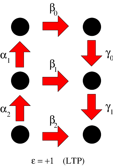

Along the lines of Fusi et al [13], the transition probabilities of both models are assumed to decay exponentially with level depth :
| (2.1) |
The corresponding characteristic length,
| (2.2) |
is one of the key ingredients of the models, which measures the number of fast levels at the top of the synapse. It will be referred to as the dynamical length of the problem. The choice made in [13] corresponds to , i.e., . A different characteristic length, the static length , giving the number of occupied levels in the default state of the synapse, will be introduced in Section 4.
3 Formalism
We will make a detailed comparative analysis of Model I and Model II, with a view to establishing similarities and differences associated with their respective architectures. In both cases the synapse is considered to be infinitely deep, with levels numbered by We use the language of stochastic processes [19], and in particular the formalism of inhomogeneous Markov chains.11 1 This formalism is a discrete-time analogue of that used extensively in the mathematical literature, to study e.g. birth and death processes or queuing processes [20, 21].
The basic quantities are the probabilities (resp. ) for the synapse to be in the state (resp. in the state) at level at time These probabilities can be combined in order to form quantities of interest:
Probability for the synapse to be in the state (resp. in the state) at time , irrespective of level:
| (3.1) |
Probability of being at level at time , irrespective of state:
| (3.2) |
Mean level depth
| (3.3) |
Level-resolved polarisation (output signal) of level and total polarisation of the synapse at time :
| (3.4) |
We have the inequalities
| (3.5) |
The probabilities and obey the following dynamical equations, whose form is characteristic of Markov chains:
Model I, (see Figure 1, left):
| (3.6) |
Model I, (see Figure 1, right):
| (3.7) |
with
| (3.8) |
Model II, (see Figure 2, left):
| (3.9) |
Model II, (see Figure 2, right):
| (3.10) |
4 Default state and parameter space
We here investigate the default state of the synapse, which is the average stationary state in the presence of a white-noise input signal. White-noise input is defined by choosing at each time step
| (4.1) |
In the presence of a random input , the probabilities and are themselves random. We first evaluate the average response of the synapse, encoded in the mean values of and with respect to the random input signal. For simplicity, we continue to use the notation and for the average probabilities, and and for their sums and differences. As the values of the input signal are independent of each other, the equations obeyed by the mean probabilities are the arithmetical means of (3.6) and (3.7) for Model I, and of (3.9) and (3.10) for Model II. The quantities and characterising the average response therefore obey:
Model I:
| (4.2) |
with
| (4.3) |
Model II:
| (4.4) |
The default state is characterised by the time-independent solution to (4.2) or (4.4). The latter is of the form
| (4.5) |
i.e.,
| (4.6) |
The default state is appropriately featureless. It is unpolarised, as it should be for a symmetric synapse. Furthermore, the occupation probabilities obey a simple exponential falloff as a function of level depth. The corresponding characteristic length,
| (4.7) |
is referred to as the static length of the problem, and gives a measure of the effective number of occupied levels in the default state. The regime of most interest is where is moderately large, so that the default state extends over several levels. The mean level depth
| (4.8) |
is then essentially given by the static length.
The key role played by two characteristic lengths, static () and dynamic (), is a striking similarity between this model and that of a column of interacting grains investigated previously [22].
In contrast to the dynamical length , which is a free parameter, the static length is related to the values of the parameters , , and in a model-dependent way. Thus:
Model I:
| (4.9) |
Model II:
| (4.10) |
The above equations reveal the main difference between the two models at the level of the default state. The stationarity of the latter state involves balancing out ‘upward’ and ‘downward’ moves arbitrarily deep within the system. This goal is achieved in different ways in both models, consistent with their structural differences.
In Model II, a large static length is reached, irrespective of , when and are nearly equal, with a small bias in the upward direction:
| (4.11) |
The situation is very different for Model I, where non-local reinjection plays a key role. The stationary profile of the response may become critical (i.e., ) when a strong local downward bias is compensated by strongly non-local upward moves:
| (4.12) |
This phenomenon is already at work in the original model by Fusi et al, where .
We now discuss the parameter space of both models. The essential parameters are the static and dynamical lengths and , whose typical values are a few units. For fixed and , , , and are related by (4.9) or (4.10). We choose to take and as our independent parameters. Besides the condition that each of them is between 0 and 1, they also fulfil (i) and (ii) (see (3.6) or (3.9) for ). For each model, the admissible values of and belong to a quadrangular domain EFGH, shown in Figure 3 for . In both cases, saturating condition (ii) yields the EH line. The non-trivial coordinates of the vertices as well as some special features, in the case of each model, are given below.


Model I:
| (4.13) |
The maximal value of for a fixed lies on the FG line. This is the defining line for the original model of Fusi et al, corresponding to the choice :
| (4.14) |
Model II:
| (4.15) |
The maximal value of for a fixed lies on the (broken) EHG line:
| (4.16) |
The above expressions (4.14) and (4.16) for cross at the following critical value of :
| (4.17) |
so that Model I has a smaller (resp. larger) for (resp. ). This is a result to bear in mind, as it turns out that the behaviour of many quantities of interest is largely determined by (see e.g. Figures 11 and 12).
Throughout the following, in numerical illustrations we use the parameter values
| (4.18) |
unless otherwise stated. For , we have , so that the chosen value of is smaller than . We have for Model I and for Model II.
5 Response to LTP input signals: power-law forgetting
5.1 Single LTP signal
When a single LTP input signal is applied at time to the synapse in its default state, it will get polarised in response, and thus ‘learn’ the signal. Later on, under the influence of a white-noise random input signal for times , it will forget the LTP signal, and return to its default state. We will show that the process of forgetting is robust with respect to the architectural differences between the two models, and is characterised by a universal power law.
The polarised probability profile of the synapse at time is obtained by acting once with equation (3.6) or (3.9) onto the default state (4.6). We thus obtain
Model I:
| (5.1) |
Model II:
| (5.2) |
The instantaneous output signal, i.e., the total polarisation of the synapse just after the LTP signal, takes the same value proportional to for both models:
| (5.3) |
For we have .
The synapse then evolves under the influence of a white-noise random input during the subsequent forgetting phase. This evolution is described for Model I by the action of the recursion (4.2) on the probabilities (5.1), and for Model II by the action of (4.4) on (5.2). Figure 4 shows plots of the reduced polarisation signals against time for Model I (left) and Model II (right), for several values of . For small enough , the polarisation overshoots, i.e., it keeps increasing beyond in a transient regime at the beginning of the forgetting phase. The duration of this transient overshoot gets larger for smaller , and formally diverges in the limit.


This paradoxical behaviour can be explained as follows. In the forgetting phase, the total polarisation obeys the balance equation
| (5.4) |
Generically, then, decays to zero, as expected. It may however grow in a transient regime, leading to the overshoot mentioned above, provided the initial polarisation profile is inhomogeneous enough so as to satisfy both
| (5.5) |
For a single LTP signal, the initial profile at time is such that , whereas for , for both models and with small (see (5.1), (5.2)). Since the rates fall off exponentially in , the initial profile is thus likely to obey the inequalities (5.5), thus leading to the overshoot. In fact, it can be shown that the overshoot always occurs for , where:
Model I:
| (5.6) |
To summarise, the instantaneous response to an LTP signal is proportional to , and therefore larger for larger ; its subsequent decay is, however, fast for large – an undesirable feature – whereas it is slow and even non-monotonic for smaller . This suggests the absence of a natural criterion for defining an optimal , where quick learning and slow forgetting might simultaneously occur at the synapse.
5.2 Universal power-law forgetting
The asymptotic fall-off of the total polarisation of the synapse in response to a single LTP signal is illustrated in Figure 5, showing a log-log plot of for much longer times (up to ). The data for both our models show a common power-law decay: thus, for our choice of parameter values, in both cases.22 2 Corrections to the asymptotic power law are, however, stronger for Model I. This is known as power-law forgetting, which will be analysed below.


The expressions (5.1), (5.2) show that the initial polarisation profile decays exponentially as a function of level depth , as
| (5.8) |
This exponential decay is governed by the product of the probabilities in the default state (see (4.6)) and the polarising rate (see (2.1)).
Now consider the synapse at a late stage of the forgetting phase (). The white-noise input essentially erases the polarisation profile down to a level depth such that . More details on this derivation can be found in Appendix A. This gives:
| (5.9) |
Of course, the only part of the polarisation that survives at large times is the part which has not yet been forgotten: this lives in the deeper levels (), where white noise has not yet erased the remnants of the memory. The total polarisation is therefore expected to scale as . Using the estimates (5.8) and (5.9), we obtain an asymptotic power-law decay of the polarisation signal:
| (5.10) |
with
| (5.11) |
The forgetting exponent thus obtained only depends on the ratio of the static and dynamical lengths and . Its expression (5.11) is universal, in the sense that it holds irrespective of the model architecture, and of the rates , , and , besides the fact that is related to the latter parameters in a model-dependent way (see (4.9), (4.10)). We would thus expect power-law forgetting with exponent to be manifested for a large class of learnt signals.
It is worth remarking here that, if the synapse were finite rather than infinite, and consist of levels, the power-law decay (5.10) would be exponentially cutoff at a time such that . The cutoff timescale thus obtained,
| (5.12) |
is exponentially large in the ratio of the number of levels to the dynamical length .
5.3 DC signal (sustained LTP signal)
We now turn to the investigation of a DC input signal, i.e., a sustained LTP input signal lasting for time steps ( for ). The synapse is again assumed to be initially in its default state.
The learning and forgetting processes will be qualitatively similar to the above, while novel qualitative features emerge deep in the DC regime, i.e., when the duration of the LTP signal is long enough so that the product is large. In this regime, the synapse gets almost totally polarised under the persistent action of the input signal. This saturation phenomenon is illustrated in Figure 6, which shows the total polarisation of both models for several durations of the DC signal.


The synapse slowly builds up a long-term memory in the presence of a long DC signal, as the polarisation profile moves to deeper and deeper levels. This feature is illustrated in Figure 7, which shows a plot of the full polarisation profile of Model II at the end of the learning phase, for several durations of the DC signal. When the synapse becomes fully polarised in the late-time regime (), the level polarisations become approximately ; for both models, the signals travel down the synapse with exponentially decaying rates. Thus, both (3.6) and (3.9) become:
| (5.13) |
The polarisation dynamics are therefore modelled by that of the logarithmic walker (Appendix A). Thus, at the end of the learning phase (), the polarisation profile will have the form of a sharply peaked traveling wave (see (1.5)), around a mean depth which grows according to the logarithmic law (see (1.2))
| (5.14) |

We now turn to the decay of the total polarisation generated by a sustained LTP signal, deep in the DC regime. Figure 8 shows a log-log plot of for several durations of the DC signal, and much longer observation times. The polarisation decays via the universal power law (5.10), irrespective of the length of the learning phase, driving home the universality of power-law forgetting.


5.4 Non-universal transient power-law forgetting
So far, we have shown that most features of our two models of the synapse are pretty robust to their different architectures: however, in the following, we show an important phenomenon where the two models differ strongly, for a sustained or persistent signal and at larger timescales.
Figure 9 shows a log-log plot of against the time ratio , for both models in the regime where the duration of the DC signal and the observation time are both large and comparable. In the case of Model I, the data for the longer times exhibit a clear collapse, indicating a scaling behaviour of the form
| (5.15) |
which is a signature of (simple) aging [23]. The corresponding scaling function falls off as . For Model II, the decay of the total polarisation is more subtle, and exhibits two successive regimes: (i) a transient regime, where exhibits simple aging in terms of , and falls off rather rapidly; (ii) an asymptotic regime, where falls off with the universal exponent , but does not obey simple aging.


This qualitative difference between both models is investigated in detail in Appendix B, but we give a simple flavour here: suppose the synapse is in a polarised state where only the uppermost level is occupied, when the process of forgetting begins. For Model I, the polarisation always falls off with the universal forgetting exponent , whereas for Model II it falls off more rapidly, with a larger transient forgetting exponent which depends continuously on (see (2.13)). For and we have . We are thus led to the following scenario for Model II: (i) the bulk of the polarisation profile is sharply localised around the typical depth (5.14) (see Figure 7), and therefore falls off with the transient exponent ; (ii) the tail of the polarisation profile, which still has the universal exponential form (5.8) (as long as is finite), is responsible for the subsequent universal asymptotic decay.
6 Fluctuations in default state and signal-to-noise ratio
The average response of the synapse to a white-noise random input signal defines its default state, investigated in Section 4. However, there are appreciable dynamical fluctuations around this average, which are seen on plots (see Figure 10) of the mean level depth (left) and of the total polarisation (right) for Model I.33 3 Similar qualitative behaviour would be obtained for Model II. The average quantities in each case are shown as red horizontal lines, for ease of comparison. The mean polarisation vanishes, whereas the mean level depth is (see (4.8)).


The large fluctuations observed in both quantities are due to the occurrence of long ordered subsequences (patches) of LTP or of LTD events in the input signal (). Patches of duration occur with exponentially small probabilities , so that for a total observation time , the largest ordered patch has . For a time of observation , for example, we can have patches of temporal length as large as . The main effect of, say a long patch of LTP/LTD events, is that the synapse gets more and more positively/negatively polarised, with the signal penetrating to ever deeper levels along the appropriate branch. Such large fluctuations in are therefore distributed symmetrically around zero, whereas those in are toward deeper levels. Clearly, the fluctuations in both quantities should be strongly correlated and the plots show that they are.
We define the (amplitude) signal-to-noise ratio of our models as the ratio of the instantaneous single LTP signal response (see (5.3)) to the standard deviation of the spontaneous fluctuations around the default state:
| (6.1) |
Figure 11 shows a plot of the signal-to-noise ratio thus defined, against , for both models. The mean squared polarisation is measured by numerically evaluating the response of our models to a very long sequence of white noise. Both datasets essentially exhibit the same monotonic dependence on . They seem to obey the scaling behaviour at small , suggested by the forthcoming analysis of the limiting regime (see (6.4)). Conversely, is maximal at , and this maximal value is essentially determined by the range of allowed values of (see (4.14), (4.16)).

For Model I with , the signal-to-noise ratio reaches its global maximum over and , i.e., , at , i.e., at point G (see Figure 3). For Model II, the global maximum is reached in the limit, i.e., again at point G.
Optimising the signal-to-noise ratio even further necessitates allowing the lengths and to vary; is observed to reach its absolute maximum in the limit. In this regime, the polarisation reads , and it is governed by the following simple dynamical equation
| (6.2) |
for both models. In the stationary state for a white-noise input, we thus have
| (6.3) |
and finally
| (6.4) |
The signal-to-noise ratio thus obeys a quarter-of-a-circle law as a function of , and attains its absolute maximum at , irrespective of anything else.
This extreme regime is however of little interest, as all the action takes place in the uppermost level (), so that metaplasticity is lost.
7 Response to a variety of input signals
In order to examine the storage of memories in the general case, we now examine the response of our two synapse models to a variety of types of time-dependent input signals. As already mentioned in the Introduction, this section completes the systematic study of our models viewed from a physicist’s perspective as signal processing units.
7.1 AC signal
An AC signal is a perfect alternation of LTP and LTD events, represented by the input
| (7.1) |
After a short transient, the synapse reaches a stationary state, where the occupation probabilities keep oscillating in phase with the input signal, according to
| (7.2) |
The staggered probabilities and are given by the normalised solution of the following equations:
Model I:
| (7.3) |
with
| (7.4) |
Model II:
| (7.5) |
The staggered polarisation of the stationary state reads
| (7.6) |
This quantity starts increasing linearly with , as
| (7.7) |
irrespective of the model, provided parameters are the same. In the limit, (7.3) and (7.5) indeed simplify to the same equations
| (7.8) |
whose normalised solution , is therefore model-independent. We have then
| (7.9) |
For the parameters (4.18) this gives .
Figure 12 shows a plot of against for both models. For each model, is limited by . Once again we see that the staggered polarisation reaches larger values for Model II, mainly as a consequence of the larger range of allowed values of .

7.2 Coloured random signal
We next consider a coloured random input signal defined by the following rule:
| (7.10) |
with for definiteness.
The persistence probability allows this coloured random signal to interpolate between several situations described above:
the DC signal investigated in Section 5.3 is recovered for ,
the AC signal investigated in Section 7.1 is recovered for ,
The correlation function of the signal (7.10) is
| (7.11) |
The coloured signal is therefore positively correlated, or persistent, for . The corresponding characteristic time
| (7.12) |
diverges near the DC limit () as . The signal is anti-persistent, with oscillating correlations, for .
The synapse submitted to a coloured random input signal reaches a fluctuating stationary state after a relatively short transient. For a given realisation, it exhibits strong dynamical fluctuations which are qualitatively similar to those shown in Figure 10. Figure 13 shows plots of the total polarisation for two typical realisations of coloured random signal, in an anti-persistent case (, left) and in a persistent case (, right). Both the amplitude and the correlation time of the fluctuations are observed to increase with , as might be expected.


Figure 14 shows a plot of (numerically measured) stationary values of the mean depth (left) and of the mean squared polarisation (right), for both models with and 0.2 and a varying persistence probability . The mean depth starts from its lowest value in the limit, i.e., for the AC signal. It increases smoothly as a function of , and diverges logarithmically as near the DC limit ().44 4 This logarithmic law can be derived in the same spirit as (1.2) and (5.14). All the curves cross at the white-noise point (), where the result (4.8) holds irrespective of the model and of its parameters. The dependence of the mean depth on the persistence probability is far more pronounced for Model II than for Model I. The behaviour of the mean squared polarisation provides another appreciable difference between the two models. In both cases it starts increasing as a function of , from a very small value in the limit. Its behaviour as is however very different in both models. The mean squared polarisation keeps steadily increasing in the case of Model I, whereas its increase is much less pronounced for Model II, even becoming non-monotonic at high enough .


This qualitative difference between the responses of both models to highly persistent random signals can be related to the difference in their transient responses, investigated in Section 5.4. In Model II, the low-frequency components of the memory lie slightly deeper within the synapse. More importantly, they relax much faster than in Model I, as their falloff can be characterised by a larger, non-universal exponent .
7.3 Oscillatory signal
The last case we consider is that of an oscillatory input signal, which consists of alternating long blocks of LTP and LTD signals of length time steps, i.e.,
| (7.13) |
where denotes the integer part.
After a relatively short transient regime, the synapse converges toward a periodic state, where the polarisation and other quantities oscillate with the period of the input signal. Figure 15 shows a plot of the values of the mean depth (left) and of the mean squared polarisation (right), averaged over one period in the stationary state of the synapse, for both models with , against the half-period of the oscillatory signal.


These data corroborate the observations made in Section 7.2. The dependence of the mean depth on is again steeper for Model II than for Model I. The data for both models are however compatible with the common logarithmic asymptotic growth law . The mean squared polarisation is observed to increase monotonically as a function of for Model I, whereas for Model II it reaches a maximum and then smoothly decreases.
8 Discussion
In this paper, we have provided the first thorough analysis of a single synapse including the effects of metaplasticity. We used two models: Model I is an extension of the original cascade model proposed by Fusi et al [13], whereas Model II, of our own invention, has a different architecture.
Our intention was, apart from the thorough quantification of earlier ideas [12], the isolation of the mechanisms responsible for the storage of memories, and the differentiation of short- and long-term memories in response to a range of signal types. In the structure of the models we analysed, long-term memories were stored at greater ‘depths’, and therefore relatively immunised to the constant bombardment of white noise in the upper levels, which forms our everyday experience. The difference between the two models lies chiefly in the mechanism of response of the synapse to a flip in sign of the input signal. In Model I, such flips tend to cause the memory trace to be dislodged to become a short-term memory of the opposite kind, while in Model II, changes in long-term memories are allowed to be more persistent, remaining at low level depths.
Most remarkably, the same asymptotic power-law forgetting (with universal exponent ) is manifested in both models, independent of their architecture. However, the aging behaviour of the models is rather different: Model I manifests simple aging, whereas Model II may have a long transient regime, where the polarisation falls off more rapidly (with a larger, non-universal and -dependent transient forgetting exponent ), before the asymptotic power-law forgetting takes over.
The behaviour of both models has been further illustrated by their responses to a range of input signals. The two observables we focused on were the mean depth of a particular memory trace, and its polarisation. Our observations suggest that Model II allows in general for a slightly greater penetration of signals. The long-term memories thus created are however rather weaker than in the case of Model I. This weakening is to be put in perspective with the existence of the non-universal transient exponent, which is studied at length in Appendix B. Qualitatively speaking, it appears that the changing of ‘opinions’ represented by the two poles of a synapse at a relatively deep level (which is possible in Model II) has the effect of weakening the strength of a memory trace, far more than when contradictions are resolved by simply disposing of them in the short-term memories of the opposite pole.
Our results provide the first prediction of the exponent of power-law forgetting at the level of a single synapse: the intensive analysis of these relatively simple models could help to start theoretical work on more complex architectures, since of course real-life forgetting relies not just on individual synapses, but on their connections to each other and to neurons. Possible extensions of this work might involve the coupling [24] of multiple synapses of the type presented above, or include the effect of correlated signals [25]; increasing correlations in these ways might enhance the competition between the bulk and the tails of the signals deep within a metaplastic synapse.
Appendix A The logarithmic walker
The problem of the logarithmic walker is defined as follows. A particle lives on the semi-infinite chain, whose sites are labelled by the positive integers (). At each time step, if sitting at site , the particle may hop to the right () with exponentially decaying probabilities . This model can be alternatively thought of as describing a discrete-time pure birth process, which has already been considered in [26].
If we assume for definiteness that the particle starts from the origin at time , the probability for the particle to be at site at time obeys the recursion
| (1.1) |
with initial condition .
Figure 16 shows a plot of the probability profile against , for and several times . The profile is observed to form a peak around a well-defined mean position . As time goes on, the profile keeps its shape, while the mean position exhibits a very slow growth.

A first heuristic approach to estimate this growth law consists in writing down the dimensional estimate , hence the result
| (1.2) |
and the name, logarithmic walker.
A more precise approach consists of writing down the following dynamical equation for the mean position of the walker at time :
| (1.3) |
For a localised probability profile, we thus obtain approximately , which yields
| (1.4) |
in agreement with (1.2).
Turning to more quantitative analysis, we look for an asymptotic solution to (1.1) in the form of a traveling wave moving on a logarithmic time scale, i.e.,
| (1.5) |
It is worth emphasising the difference between the present situation, where time enters the argument through its logarithm and with an explicitly known prefactor , and the usual situation of ballistic traveling waves, like e.g. in the FKPP equation [27]. For such traveling waves, time is multiplied by an unknown velocity , whose determination is non-trivial, and known to be very sensitive to discretization and other fluctuation effects [28].
The hull function of the traveling wave (1.5) is found to obey the linear differential-difference equation
| (1.6) |
As a consequence, its Laplace transform
| (1.7) |
obeys the difference equation
| (1.8) |
whose normalised solution reads
| (1.9) |
where is the infinite product
| (1.10) |
The latter product has zeros on the semi-infinite lattice of points , with and integers such that , whereas shares these zeros for only.
For the time being, let us consider the characteristic function of the position , i.e., the generating function of the probabilities :
| (1.11) |
In the long-time regime, the traveling-wave form (1.5) of the probabilities translates to
| (1.12) |
where the right-hand side has been obtained by means of the Poisson summation formula.
Setting in (1.12), we obtain unity identically, as expected. The reason is that we have , whereas for ; thus, the hull function has the remarkable property that the ‘stroboscoped’ sum equals one for all values of the real variable :
| (1.13) |
The asymptotic behaviour of the mean position can be derived by expanding the result (1.12) to first order in . We thus obtain
| (1.14) |
where denotes Euler’s constant. The sum is the Fourier series of a periodic function of , with unit period. These oscillations originate in the discrete nature of the sites of the chain. They manifest themselves e.g. in the shape of the probability profile near its top. Oscillations are however extremely small for global quantities such as . Their amplitude is essentially given by the first Fourier coefficients (), which are proportional to . For , this amplitude is of order , while for it is of order .
Neglecting these (tiny) oscillations, we are left with
| (1.15) |
This expression confirms the estimates (1.2) and (1.4), and gives an explicit expression for the finite part of the logarithm, where
| (1.16) |
The Mellin-Barnes integral representation of the right-hand side, where is Riemann’s zeta function, is suited to the derivation of the expansion of in the regime of small . We thus obtain the rapidly convergent expansion
| (1.17) |
hence
| (1.18) |
The full leading term was already correctly predicted in (1.4).
A similar treatment of the second moment demonstrates that the variance of the position saturates to the asymptotic value
| (1.19) |
again up to negligibly small periodic oscillations, with
| (1.20) |
We thus obtain
| (1.21) |
hence
| (1.22) |
In both above expressions the dots stand for an exponentially small contribution, proportional to .
To close, let us come back to the form of the hull function , which describes the asymptotic shape of the probability profile. The decay of the hull function at both ends is faster than exponential, since its Laplace transform , given in (1.9), is an entire function, i.e., it is analytic in the whole plane. The decay of as can be derived by inserting the asymptotic behaviour of as in the inverse Laplace formula
| (1.23) |
For , we have . We thus obtain a double exponential decay:
| (1.24) |
For , with exponential accuracy, we have , so that . The hull function therefore falls off as a Gaussian:
| (1.25) |
Finally, in the regime of small , where the variance is large, the whole hull function is nearly Gaussian:
| (1.26) |
Appendix B Transient behaviour
This Appendix is devoted to the transient behaviour of our models. Our main goal is to show that the transient responses of both models are qualitatively different. The polarisation of Model II exhibits a non-universal power-law decay, with a transient exponent which depends continuously on (see (2.13)), whereas the polarisation of Model I always falls off with the universal exponent (see (5.11)).
To probe this further, we analyse the transient average response of the synapse to a white-noise random input. We shift time so that is the beginning of the forgetting period. For simplicity and without loss of generality, we caricature transient effects by choosing an initial state such that the transient regime will last forever. More specifically, we assume that the synapse is prepared in a totally polarised state living entirely on the uppermost level: , . We will successively consider the level occupation probabilities and the level-resolved and total polarisations.
Level occupation probabilities
We begin with the level occupation probabilities . The following scenario is expected in the long-time regime: the should converge rather fast to their stationary values (see (4.5)) at moderate level depths, whereas their values at very deep levels should fall off more rapidly, as these are unaffected by the random input.
From a quantitative viewpoint, along the lines of (1.5), we look for an asymptotic long-time solution to (4.2) or (4.4) for the in the form of a traveling wave (front) moving on a logarithmic time scale:
| (2.1) |
The scaling function is expected to decrease from 1 in the limit to 0 in the limit. Both models have to be dealt with separately.
Model I:
The function describing the front obeys the equation
| (2.2) | |||||
Along the lines of Appendix A, we introduce the Laplace transform of , which obeys the functional equation
| (2.3) |
The expected behaviour of implies that is analytic for and has a simple pole at with unit residue (i.e., ). The property that has no pole at implies that the expression inside the parentheses on the right-hand side of (2.3) vanishes for . We thus recover (4.9). The function can be given as an explicit expression similar to (1.9), involving two infinite products, which will not be needed in the following.
Model II:
The analysis is very similar. The function obeys the equation
| (2.4) | |||||
The Laplace transform obeys
| (2.5) |
The absence of a pole at implies . We thus recover (4.10).
Level-resolved and total polarisations
We now turn to the analysis of the level-resolved polarisations and of the total polarisation . We anticipate a power-law decay in the long-time regime. Thus, we look for an asymptotic solution to (4.2) or (4.4) for the in the form of a power-law decay, with a positive exponent , which multiplies a logarithmic front:
| (2.6) |
The scaling function is expected to decrease fast enough as , in such a way that the total polarisation of the synapse also falls off as . Both models again have to be dealt with separately.
Model I:
The function obeys the equation
| (2.7) | |||||
The Laplace transform of obeys the functional equation
| (2.8) | |||||
The fast decay of as implies that is analytic at least for . The absence of a pole at yields . Using (4.9), this condition simplifies to
| (2.9) |
The vanishing of the first factor55 5 The second factor of (2.9) is positive, as a consequence of (4.9). leads to the simple result that is identical to the universal forgetting exponent (see (5.11)). We have thus shown that Model I exhibits a remarkably universal power-law forgetting.
Model II:
The analysis is similar, although it leads to a very different outcome. The function obeys the equation
| (2.10) | |||||
The Laplace transform of obeys the functional equation
| (2.11) | |||||
The absence of a pole at yields . Using (4.10), this condition simplifies to
| (2.12) |
In contrast to Model I, we now obtain a transient forgetting exponent
| (2.13) |
which depends continuously on . It turns out to be a strongly increasing function of , starting from the universal value in the limit as
| (2.14) |
and reaching its maximum for (see (4.16)). Figure 17 shows a plot of against for the parameters (4.18).

The occurrence of the non-trivial equation (2.12) for the exponent in the case of Model II can be traced back to the difference in architecture between both models. For Model I, where -transitions involve a non-local reinjection to the uppermost level, the rates multiplying and for generic in the right-hand side of (4.2) are identical and involve the combination . For Model II, where -transitions take place locally at any depth, the rates multiplying and for generic in the right-hand side of (4.4) are different, as they are respectively proportional to and , so that locally the polarisation relaxes more rapidly than the level occupation .
Finally, the conclusions of this Appendix regarding the forgetting exponents hold more generally as soon as the level occupation probabilities in the initial state fall off exponentially more rapidly than the profile (4.5) of the default state.
References
References
- [1] Ebbinghaus H, 1913 Memory: A contribution to experimental psychology (H A Ruger & C E Bussenius, translators) (New York: Teachers College Press, Columbia University) (Original work published 1885; reprint of translation published by Dover, New York, 1964)
- [2] Amit D J, Gutfreund H, and Sompolinsky H, 1985 Phys. Rev. Lett. 55 1530
- [3] Amit D J and Fusi S, 1992 Network: Computation in Neural Systems 3 443 Amit D J and Fusi S, 1994 Neural Computation 6 957 Amit D J and Brunel N, 1997 Network: Computation in Neural Systems 8 373
- [4] Amit D J, 1999 Modeling Brain Function: The World of Attractor Neural Networks (Cambridge: Cambridge University Press)
- [5] Gardner E and Derrida B, 1988 J. Phys. A 21 271 Gardner E and Derrida B, 1989 J. Phys. A 22 1983
- [6] Hopfield J J, 1984 Proc. Natl Acad. Sci. USA 81 3088 Hopfield J J, 2008 Neural Computation 20 1119 Hopfield J J, 2010 Proc. Natl Acad. Sci. USA 107 1648
- [7] Petersen C C H, Malenka R C, Nicoll R A, and Hopfield J J, 1998 Proc. Natl Acad. Sci. USA 95 4732
- [8] O’Connor D H, Wittenberg G M, and Wang S S H, 2005 Proc. Natl Acad. Sci. USA 102 9679
- [9] Fusi S and Senn W, 2006 Chaos 16 026112 Fusi S and Abbott L F, 2007 Nature Neuroscience 10 485
- [10] Baldassi C, Braunstein A, Brunel N, and Zecchina R, 2007 Proc. Natl Acad. Sci. USA 104 11079
- [11] Barrett A B and van Rossum M C W, 2008 PLoS Computational Biology 4 e1000230
- [12] Fusi S, 2002 Biological Cybernetics 87 459
- [13] Fusi S, Drew P J, and Abbott L F, 2005 Neuron 45 599
- [14] Wixted J T and Ebbesen E B, 1991 Psychological Science 2 409 Wixted J T and Ebbesen E B, 1997 Memory & Cognition 25 731
- [15] Kello C T, Brown G D A, Ferrer-I-Cancho R, Holden J G, Linkenkaer-Hansen K, Rhodes T, and van Orden G C, 2010 Trends Cogn. Sci. 14 223
- [16] Dayan P and Abbott L F, 2001 Theoretical Neuroscience: Computational and Mathematical Modeling of Neural Systems (Cambridge: MIT Press) Gerstner W and Kistler W M, 2002 Spiking Neuron Models: Single Neurons, Populations, Plasticity (Cambridge: Cambridge University Press)
- [17] Abraham W C and Bear M F, 1996 Trends in Neurosciences 19 126
- [18] Fischer T M, Blazis D E J, Priver N A, and Carew T J, 1997 Nature 389 860
- [19] van Kampen N G, 1992 Stochastic Processes in Physics and Chemistry (Amsterdam: North-Holland)
- [20] Feller W, 1968 An Introduction to Probability Theory and its Applications (New York: Wiley)
- [21] Karlin S and Taylor H M, 1975 A First Course in Stochastic Processes (New York: Academic)
- [22] Mehta A and Luck J M, 2003 J. Phys. A 36 L365 Luck J M and Mehta A, 2003 Eur. Phys. J. B 35 399 Luck J M and Mehta A, 2007 Eur. Phys. J. B 57 429 Luck J M and Mehta A, 2010 Eur. Phys. J. B 77 505
- [23] Cugliandolo L F, 2004 in Slow Relaxations and Nonequilibrium Dynamics in Condensed Matter, 2004 Les Houches – Ecole d’Eté de Physique Théorique vol 77 ed J L Barrat et al (Berlin: Springer) Also available as [cond-mat/0210312]
- [24] Mahajan G and Mehta A, 2011 Europhys. Lett. 95 48008 Mahajan G and Mehta A, 2011 Europhys. Lett. 95 69901 Bhat A A, Mahajan G, and Mehta A, 2011 PLoS ONE 6(9) e25048
- [25] van Rossum M C W and Turrigiano G G, 2001 Neurocomputing 38 409
- [26] Grimmett G R, 1975 J. Appl. Probab. 12 673
- [27] Fisher R A, 1937 Annals of Eugenics 7 355 Kolmogorov A N, Petrovsky I G, and Piskunov N S, 1937 Moscow Univ. Bull. Math. 1 1
- [28] Brunet E and Derrida B, 1997 Phys. Rev. E 56 2597 Brunet E and Derrida B, 2004 Phys. Rev. E 70 016106