Celerity: A Low-Delay Multi-Party Conferencing Solution
Abstract
In this paper, we attempt to revisit the problem of multi-party conferencing from a practical perspective, and to rethink the design space involved in this problem. We believe that an emphasis on low end-to-end delays between any two parties in the conference is a must, and the source sending rate in a session should adapt to bandwidth availability and congestion. We present Celerity, a multi-party conferencing solution specifically designed to achieve our objectives. It is entirely Peer-to-Peer (P2P), and as such eliminating the cost of maintaining centrally administered servers. It is designed to deliver video with low end-to-end delays, at quality levels commensurate with available network resources over arbitrary network topologies where bottlenecks can be anywhere in the network. This is in contrast to commonly assumed P2P scenarios where bandwidth bottlenecks reside only at the edge of the network. The highlight in our design is a distributed and adaptive rate control protocol, that can discover and adapt to arbitrary topologies and network conditions quickly, converging to efficient link rate allocations allowed by the underlying network. In accordance with adaptive link rate control, source video encoding rates are also dynamically controlled to optimize video quality in arbitrary and unpredictable network conditions. We have implemented Celerity in a prototype system, and demonstrate its superior performance over existing solutions in a local experimental testbed and over the Internet.
1 Introduction
With the availability of front-facing cameras in high-end smartphone devices (such as the Samsung Galaxy S and the iPhone 4), notebook computers, and HDTVs, multi-party video conferencing, which involves more than two participants in a live conferencing session, has attracted a significant amount of interest from the industry. Skype, for example, has recently launched a monthly-paid service supporting multi-party video conferencing in its latest version (Skype 5) [1]. Skype video conferencing has also been recently supported in a range of new Skype-enabled televisions, such as the Panasonic VIERA series, so that full-screen high-definition video conferencing can be enjoyed in one’s living room. Moreover, Google has supported multi-party video conferencing in its latest social network service Google+. And Facebook cooperating with Skype plans to provide video conferencing service to its billions of users. We argue that these new conferencing solutions have the potential to provide an immersive human-to-human communication experience among remote participants. Such an argument has been corroborated by many industry leaders: Cisco predicts that video conferencing and tele-presence traffic will increase ten-fold between 2008-2013 [2].
While traffic flows in a live multi-party conferencing session are fundamentally represented by a multi-way communication process, today’s design of multi-party video conferencing systems are engineered in practice by composing communication primitives (e.g., transport protocols) over uni-directional feed-forward links, with primitive feedback mechanisms such as various forms of acknowledgments in TCP variants or custom UDP-based protocols. We believe that a high-quality protocol design must harness the full potential of the multi-way communication paradigm, and must guarantee the stringent requirements of low end-to-end delays, with the highest possible source coding rates that can be supported by dynamic network conditions over the Internet.
From the industry perspective, known designs of commercially available multi-party conferencing solutions are either largely server-based, e.g., Microsoft Office Communicator, or are separated into multiple point-to-point sessions (this approach is called Simulcast), e.g., Apple iChat. Server-based solutions are susceptible to central resource bottlenecks, and as such scalability becomes a main concern when multiple conferences are to be supported concurrently. In the Simulcast approach, each user splits its uplink bandwidth equally among all receivers and streams to each receiver separately. Though simple to implement, Simulcast suffers from poor quality of service. Specifically, peers with low upload capacity are forced to use a low video rate that degrades the overall experience of the other peers.
In the academic literature, there are recently several studies on peer-to-peer (P2P) video conferencing from a utility maximization perspective [3, 4, 5, 6, 7, 8]. Among them, Li et al. [3] and Chen et al. [4] may be the most related ones to this work (we call their unified approach Mutualcast). They have tried to support content distribution and multi-party video conferencing in multicast sessions, by maximizing aggregate application-specific utility and the utilization of node uplink bandwidth in P2P networks. Specific depth-1 and depth-2 tree topologies have been constructed using tree packing, and rate control was performed in each of the tree-based one-to-many sessions.However, they only considered the limited scenario where bandwidth bottlenecks reside at the edge of the network, while in practice bandwidth bottlenecks can easily reside in the core of the network [9, 10]. Further, all existing industrial and academic solutions, including Mutualcast, did not explicitly consider bounded delay in designs, and can lead to unsatisfied interactive conferencing experience.
1.1 Contribution
In this paper, we reconsider the design space in multi-party video conferencing solutions, and present Celerity, a new multi-party conferencing solution specifically designed to maintain low end-to-end delays while maximizing source coding rates in a session. Celerity has the following salient features:
- •
It operates in a pure P2P manner, and as such eliminating the cost of maintaining centrally administered servers.
- •
It can deliver video at quality levels commensurate with available network resources over arbitrary network topologies, while maintaining bounded end-to-end delays.
- •
It can automatically adapt to unpredictable network dynamics, such as cross traffic and abrupt link failures, allowing smooth conferencing experience.
Enabling the above features for multi-party conferencing is challenging. First, it requires a non-trivial formulation that allows systematic solution design over arbitrary network capacity constraints. In contrast, existing P2P system design works with performance guarantee commonly assume bandwidth bottlenecks reside at the edge of the network. Second, maximizing session rates subject to bounded delay is known to be NP-Complete and hard to solve approximately [11]. We take a practical approach in this paper that explores all -hop delay-bounded overlay trees with polynomial complexity. Third, detecting and reacting to network dynamics without a priori knowledge of the network conditions are non-trivial. We use both delay and loss as congestion measures and adapt the session rates with respect to both of them, allowing early detection and fast response to unpredictable network dynamics.
The highlight in our design is a distributed rate control protocol, that can discover and adapt to arbitrary topologies and network conditions quickly, converging to efficient link rate allocations allowed by the underlying network. In accordance with adaptive link rate control, source video encoding rates are also dynamically controlled to optimize video quality in arbitrary and unpredictable underlay network conditions.
The design of Celerity is largely inspired by our new formulation that specifically takes into account arbitrary network capacity constraints and allows us to explore design space beyond those in existing solutions. Our formulation is overlay link based and has a number of variables linear in the number of overlay links. This is a significant reduction as compared to the number of variables exponential in the number of overlay links in an alternative tree-based formulation. We believe our approach is applicable to other P2P system problems, to allow solution design beyond the common assumption in P2P scenarios that the bandwidth bottlenecks reside only at the edge of the network.
We have implemented a prototype Celerity system using C++. By extensive experiments in a local experimental testbed and on the Internet, we demonstrate the superior performance of Celerity over state-of-the-art solutions Simulcast and Mutualcast.
1.2 Paper Organization
The rest of this paper is organized as follows. In Section 2, we introduce a general formulation for the multi-party conferencing problem; existing solutions can be considered as algorithms solving its special cases. We present and discuss the designs of two critical components of Celerity, the tree packing module and the link rate control module, in Sections 3 and 4, respectively. We present the practical implementation of Celerity in Section 5 and the experimental results in Section 6. Finally, we conclude in Section 7. We leave all the proofs and pseudo codes in the Appendix.
2 Problem Formulation and Celerity Overview
One way to design a multi-party conferencing system is to formulate its fundamental design problem, explore powerful theoretical techniques to solve the problem, and use the obtained insights to guide practical system designs. In this way, we can also be clear about potential and limitation of the designs, allowing easy system tuning and further systematic improvements. Table 1 lists the key notations used in this paper.
| Notation | Definition |
|---|---|
| Set of all physical links | |
| Set of conference participating nodes | |
| Set of directed overlay links | |
| Capacity of the physical link | |
| Whether overlay link passes physical link | |
| Rate allocated to session on overlay link | |
| Overlay link rates of stream , | |
| Overlay link rates of all streams, | |
| Total overlay link traffics, | |
| Delay bound | |
| Session ’s rate within the delay bound | |
| Price function of violating link ’s capacity constraint | |
| Lagrange multiplier of link ’s capacity constraint | |
| Lagrange function of variables and |
Note: we use bold symbols to denote vectors.
2.1 Settings
Consider a network modeled as a directed graph , where is the set of all physical nodes, including conference participating nodes and other intermediate nodes such as routers, and is the set of all physical links. Each link has a nonnegative capacity and a nonnegative propagation delay .
Consider a multi-party conferencing system over . We use to denote the set of all conference participating nodes. Every node in is a source and at the same time a receiver for every other nodes. Thus there are totally sessions of (audio/video) streams. Each stream is generated at a source node, say , and needs to be delivered to all the rest nodes in , by using overlay links between any two nodes in .
An overlay link means can send data to by setting up a TCP/UDP connection, along an underlay path from to pre-assigned by routing protocols. Let be the set of all directed overlay links. For all and , we define
| (1) |
The physical link capacity constraints are then expressed as
where denotes the rate allocated to session on overlay link and describes the total overlay traffic passing through physical link .
Remark: In our model, the capacity bottleneck can be anywhere in the network, not necessarily at the edges. This is in contrast to a common assumption made in previous P2P works that the uplinks/downlinks of participating nodes are the only capacity bottleneck.
2.2 Problem Formulation
In a multi-party conferencing system, each session source broadcasts its stream to all receivers over a complete overlay graph on which every link has a rate and a delay . For smooth conferencing experience, the total delay of delivering a packet from the source to any receiver, traversing one or multiple overlay links, cannot exceed a delay bound .
A fundamental design problem is to maximize the overall conferencing experience, by properly allocating the overlay link rates to the streams subject to physical link capacity constraints. We formulate the problem as a network utility maximization problem:
| (2) | |||||
| s.t. | (3) |
The optimization variables are and the constraints in (3) are the physical link capacity constraints.
denotes session ’s rate that we obtain by using resource within the delay bound , and is a concave function of as we will show in Corollary 1 in the next section.
The objective is to maximize the aggregate system utility. is an increasing and strictly concave function that maps the stream rate to an application-specific utility. For example, a commonly used video quality measure Peak Signal-to-Noise Ratio (PSNR) can be modeled by using a logarithmic function as the utility [4] 11 1 Using logarithmic functions also guarantees (weighted) proportional fairness among sessions and thus no session will starve at the optimal solution [12].. With these settings and observations, is concave in and the problem MP is a concave optimization problem.
Remarks: (i) The formulation of MP is an overlay link based formulation in which the number of variables per session is and thus at most . One can write an equivalent tree-based formulation for MP but the number of variables per session will be exponential in and . (ii) Existing solutions, such as Simulcast and Mutualcast, can be thought as algorithms solving special cases of the problem MP. For example, Simulcast can be thought as solving the problem MP by using only the -hop tree to broadcast content within a session. Mutualcast can be thought as solving a special case of the problem MP (with the uplinks of participating nodes being the only capacity bottleneck) by packing certain depth-1 and depth-2 trees within a session.
2.3 Celerity Overview
Celerity builds upon two main modules to maximize the system utility: (1) a delay-bounded video delivery module to distribute video at high rate given overlay link rates (i.e., how to compute and achieve ); (2) a link rate control module to determine .
Video delivery under known link constraints: This problem is similar to the classic multicast problem, and packing spanning (or Steiner) trees at the multicast source is a popular solution. However, the unique “delay-bounded” requirement in multi-party conferencing makes the problem more challenging. We introduce a delay-bounded tree packing algorithm to tackle this problem (detailed in Section 3).
Link rate control: In principle, one can first infer the network constraints and then solve the problem MP centrally. However, directly inferring the constraints potentially requires knowing the entire network topology and is highly challenging. In Celerity, we resort to design adaptive and iterative algorithms for solving the problem MP in a distributed manner, without a priori knowledge of the network conditions (detailed in Section 4).
We high-levelly explain how Celerity works in a 4-party conferencing example in Fig. 1. We focus on session , in which source distributes its stream to receivers , , and , by packing delay-bounded trees over a complete overlay graph shown in the figure. We focus on source and one overlay link , which represents a UDP connection over an underlay path to to to . Other overlay links and other sessions are similar.
We first describe the control plane operations. For the overlay link , the head node works with the tail node to periodically adjust the session rate according to Celerity’s link rate control algorithm. Such adjustment utilizes control-plane information that source piggybacks with data packets, and loss and delay statistics experienced by packets traveling from to . We show such local adjustments at every overlay link result in globally optimal session rates.
The head node also periodically reports to source the session rate and the end-to-end delay from to . Based on these reports from all overlay links, source periodically packs delay-bounded trees using Celerity’s tree-packing algorithm, calculates necessary control-plane information, and delivers data and the control-plane information along the trees.
The data plane operations are simple. Celerity uses delay-bounded trees to distribute data in a session. Nodes on every tree forward packets from its upstream parent to its downstream children, following the “next-children” tree-routing information embedded in the packet header. Celerity’s tree-packing algorithm guarantees that (i) packets arrive at all receivers within the delay bound, and (ii) the total rate of a session passing through an overlay link does not exceed the allocated rate .
In the following two sections, we first present the designs of the two main modules in Celerity. We then describe how they are implemented in physical peers in Section 5.
3 Packing Delay-bounded Trees
Given the link rate vector and delay for every overlay link (i.e.,), achieving the maximum broadcast/multicast stream rate under a delay bound is a challenging problem. A general way to explore the broadcast/multicast rate under delay bounds is to pack delay-bounded Steiner trees. However, such problem is -hard [13]. Moreover, the number of delay-bounded Steiner trees to consider is in general exponential in the network size.
In this paper, we pack -hop delay-bounded trees in an overlay graph of session , denoted by , to achieve a good stream rate under a delay bound. Note by graph theory notations, a -hop tree has a depth at most . Packing -hop trees is easy to implement. It also explores all overlay links between source and receiver and between receivers, thus trying to utilize resource efficiently. In fact, it is shown in [4, 3] that packing -hop multicast trees suffices to achieve the maximum multicast rate for certain P2P topologies. We elaborate our tree-packing scheme in the following.
We first define the overlay graph . Graph is a directed acyclic graph with two layers; one example of such graph is illustrated in Fig. 2. In this example, consider a session with a source , three receivers . For each receiver , we draw two nodes, and , in the graph ; models the receiving functionality of node and models the relaying functionality of node .
Suppose that the prescribed link bit rates are given by the vector , with the capacity for link being . Then in , the link from to has capacity , the link from to (with ) has capacity , and the link from to has infinite capacity. If the propagation delay of an edge exceeds the delay bound, we do not include it in the graph. If the propagation delay of a two-hop path exceeds the delay bound, we omit the edge from to from the graph. As a result, every path from to any receiver in the graph has a path propagation delay within the delay bound.

Over such -layer sub-graph , we pack -hop trees connecting the source and every receiver using the greedy algorithm proposed in [14]. Below we simply describe the algorithm and more details can be found in [14].
Assuming all edges have unit-capacity and allowing multiple edges for each ordered node pair. The algorithm packs unit-capacity trees one by one. Each unit-capacity tree is constructed by greedily constructing a tree edge by edge starting from the source and augmenting towards all receivers. It is similar to the greedy tree-packing algorithm based on Prim’s algorithm. The distinction lies in the rule of selecting the edge among all potential edges. The edge whose removal leads to least reduction in the multicast capacity of the residual graph is chosen in the greedy algorithm.
We show a simple example to illustrate how the tree packing algorithm works. Fig. 3 shows the process of packing a unit-capacity tree over a -layer sub-graph. In this example, is source and , , are three receivers, each edge from to and from to has unit capacity. The associated with the edge between and means the edge has infinite capacity.
The tree packing algorithm maintains a “connected set”, denoted by , that contains all the nodes that can be reached from during the tree construction process. Initially, contains only the source . In each step, the algorithm adds and connects one more node to the tree and appends the node into . The algorithm finds a tree when contains all the receivers.
Seen from Fig. 3, in Step 1, the algorithm evaluates the links starting from source and greedily picks the edge whose removal gives the smallest reduction of the multicast capacity in the residual graph. In this example, any edge leaving can be chosen because their removals give the same reduction. Our algorithm randomly picks one such equally-good edge, in this case say edge . The algorithm adds node into and amends it to be .
In Step 2, the algorithm evaluates the edges originated from any node in . In this case it picks edge and amends to be . The algorithm repeats the process until all the receivers are in , which is Step 4 in this example. The algorithm then successfully constructs a unit-capacity tree . Afterwards, the algorithm resets and constructs next tree in the residual graph until no unit-capacity tree can be further constructed.

The above greedy algorithms is very simple to implement and its practical implementation details are further discussed in Section 5.
Utilizing the special structure of the graph , we obtain performance guarantee of the algorithm as follows.
Theorem 1
The tree-packing algorithm in [14] achieves the minimum of the min-cuts separating the source and receivers in and is expressed as
| (4) |
Furthermore, the algorithm has a running time of .
Proof: Refer to Appendix A.
Hence, our tree-packing algorithm achieves the maximum delay-bounded multicast rate over the -layer sub-graph . The achieved rate is a concave function of as summarized below.
Corollary 1
The delay-bounded multicast rate obtained by our tree-packing algorithm is a concave function of the overlay link rates .
Proof: Refer to Appendix B.
3.1 Pack Delay-bounded Trees With Helpers Existing
In the previous discussion, we do not involve helpers(a helper node is neither a source nor a receiver in the conferencing session, but it is willing to help in distributing content) in our tree packing algorithm. Actually, this tree packing algorithm can also achieve the minimum of the min-cuts separating the source and receivers in even though there exist helpers.
To see how the tree packing algorithm can be applied to which includes helpers, we firstly define the 2-layer sub-graph with helpers existing; one example of such graph is illustrated in Fig. 4. In this example, consider a session with a source , three receivers , and a heper . Similarly, for each receiver , we draw two nodes, and , in the graph ; models the receiving functionality of node and models the relaying functionality of node .

Suppose that the prescribed link bit rates are given by the vector , with the capacity for link being . Then in , the link from to has capacity , the link from to (with ) has capacity , and the link from to has infinite capacity. Similarly, the link from to (a helper) has capacity and the link from to has capacity . If the propagation delay of an edge exceeds the delay bound, we do not include it in the graph. If the propagation delay of a two-hop path exceeds the delay bound, we omit the edge from to from the graph. As a result, every path from to any receiver in the graph has a path propagation delay within the delay bound.
Over such -layer sub-graph , we use the same greedy tree packing algorithm to pack -hop trees connecting the source and every receiver, and it can still achieve the minimum of the min-cuts separating the source and receivers in , which is discribed as follows.
Theorem 2
The tree-packing algorithm in [14] achieves the minimum of the min-cuts separating the source and receivers in with helpers existing and is expressed as
| (5) |
Furthermore, the algorithm has a running time of .
Proof: Refer to Appendix A.
Similarly, the achieved rate is a concave function of as summarized below.
Corollary 2
In the 2-layer sub-graph with helpers existing, the delay-bounded multicast rate obtained by our tree-packing algorithm is a concave function of the overlay link rates .
Proof: Refer to Appendix B.
4 Overlay Link Rate Control
4.1 Considering Both Delay and Loss
We revise original formulation to design our link rate control algorithm with both queuing delay and loss rate taken into account. Adapting link rates to both delay and loss allows early detection and fast response to network dynamics.
Consider the following formulation with a penalty term added into the objective function of the problem MP:
| (6) | |||||
| s.t. | (7) |
where is the penalty associated with violating the capacity constraint of physical link , and we choose the price function to be
| (8) |
where . If all the constraints are satisfied, then the second term in (6) vanishes; if instead some constraints are violated, then we charge some penalty for doing so.
Remark: (i) The problem MP-EQ is equivalent to the original problem MP. Because any feasible solution of these two problems must satisfy , and consequently the penalty term in the problem MP-EQ vanishes. Therefore, any optimal solution of the original problem MP must be an optimal solution of the problem MP-EQ and vice versa. (ii) It can be verified that is a concave function in ; hence, is a linear combination of concave functions and is concave. However, because is the minimum min-cut of the overlay graph with link rates being , is not a differentiable function [15].
We apply Lagrange dual approach to design distributed algorithms for the problem MP-EQ. The advantage of adopting distributed rate control algorithms in our system is that it allows robust adaption upon unpredictable network dynamics.
The Lagrange function of the problem is given by:
| (9) | |||||
where is the Lagrange multiplier associated with the capacity constraint in (7) of physical link . can be interpreted as the price of using link . Since the problem MP-EQ is a concave optimization problem with linear constraints, strong duality holds and there is no duality gap. Any optimal solution of the problem and one of its corresponding Lagrangian multiplier is a saddle point of and vice versa. Thus to solve the problem MP-EQ, it suffices to design algorithms to pursue saddle points of .
4.2 A Loss-Delay Based Primal-Subgradient-Dual Algorithm
There are two issues to address in designing algorithms for pursuing saddle points of . First, the utility function (and consequently ) is not everywhere differentiable. Second, (and consequently ) is not strictly concave in , thus distributed algorithms may not converge to the desired saddle points under multi-party conferencing settings [4].
To address the first concern, we use subgradient in algorithm design. To address the second concern, we provide a convergence result for our designed algorithm.
To proceed, we first compute subgradients of . The proposition below presents a useful observation.
Proposition 1
A subgradient of with respect to for any and is given by
where is a subgradient of with respect to .
Proof: Refer to Appendix C.
Motivated by the pioneering work of Arrow, Hurwicz, and Uzawa [16]
and the followup works [17][18],
we propose to use the following primal-subgradient-dual algorithm
to pursue the saddle point of :,
Primal-Subgradient-Dual Link Rate Control Algorithm:
| (10) | |||||
| (11) |
where represents a constant the step size for all the iterations, and function
We have the following observations for the control algorithm in (10)-(11):
- •
It is known that can be interpreted as the packet loss rate observed at overlay link [19]. The intuitive explanation is as follows. The term is the excess traffic rate offered to physical link ; thus models the fraction of traffic that is dropped at . Assuming the packet loss rates are additive (which is a reasonable assumption for low packet loss rates), the total packet loss rates seen by the overlay link is given by .
- •
It is also known that updating according to (11) can be interpreted as queuing delay at physical link [20]. Intuitively, if the incoming rate at , then it introduces an additional queuing delay of for . If otherwise the term , then the present queueing delay is reduced by an amount of unless hitting zero. The total queuing delay observed by the overlay link is then given by the sum .
- •
It turns out that the utility function, the subgradients, packet loss rate and queuing delay are sufficient statistics to update independently of the updates of other link rates. This way, we can solve the problem MP-EQ without knowing the physical network topology and physical link capacities.
The algorithm in (10)-(11) is similar to the standard primal-dual algorithm, but since is not differentiable everywhere, we use subgradient instead of gradient in updating the overlay link rates . If we fix the dual variables , then the algorithm in (10) corresponds to the standard subgradient method [21]. It maximizes a non-differentiable function in a way similar to gradient methods for differentiable functions — in each step, the variables are updated in the direction of a subgradient. However, such a direction may not be an ascent direction; instead, the subgradient method relies on a different property. If the variable takes a sufficiently small step along the direction of a subgradient, then the new point is closer to the set of optimal solutions.
Establishing convergence of subgradient algorithms for saddle-point optimization is in general challenging [17]. We explore convergence properties for our primal-subgradient-dual algorithm in the following theorem.
Theorem 3
Proof: Refer to Appendix D.
Remarks: (i) The results bound the time-average Lagrange function value obtained by the algorithm to the optimal in terms of distances of the initial iterates to a saddle point. In particular, the averaged function values converge to the saddle point value within a gap of , at a rate of . (ii) The requirement of the utility function is easy to satisfied; one example is with . (iii) Our results generalize the one in [17] in the sense that the one in [17] only applies to the case of uniform step size, while we allow different to update with different step size , which is critical for to be interpreted as queuing delay and thus practically measurable. Our results also have less stringent requirement on the utility function than the one in [17]. (iv) Although the results may not warranty convergence in the strict sense, our experiments over LAN testbed and on the Internet in Section 6 show the algorithm quickly stabilizes around optimal operating points. Obtaining stronger convergence results that confirm our practical observations are of great interests and is left for future work.
4.3 Computing Subgradients of
A key to implementing the Primal-Subgradient-Dual algorithm is to obtain subgradients of . We first present some preliminaries on subgradients, as well as concepts for computing subgradients for .
Definition 1
Given a convex function , a vector is said to be a subgradient of at if
where represents the domain of the function .
For a concave function , is a convex function. A vector is said to be a subgradient of at if is a subgradient of .
Next, we define the notion of a critical cut. For session , let its source be and receiver set be . A partition of the vertex set, with and for some , determines an --cut. Define
be the set of overlay links originating from nodes in set and going into nodes in set . Define the capacity of cut as the sum capacity of the links in :
Definition 2
For session , a cut is an - critical cut if it separates and any of its receivers and .
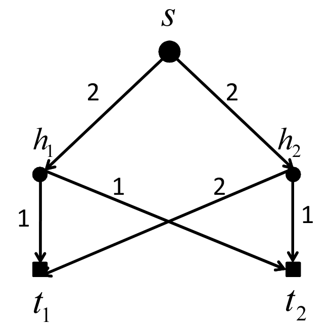
We show an example to illustrate the concept of critical cut. In Fig. 5, is a source, and , are its two receivers. The minimum of the min-cuts among the receivers is . For the cut , its contains links and , each having capacity one. Thus the cut has a capacity of and it is an critical cut.
With necessary preliminaries, we turn to compute subgradients of . Since is the minimum min-cut of and its receivers over the overlay graph , it is known that one of its subgradients can be computed in the following way [15].
- •
Find an - critical cut for session , denote it as . Note there can be multiple - critical cuts in graph , and it is sufficient to find any one of them.
- •
A subgradient of with respect to is given by
(12)
In our system, these subgradients are computed by the source of each session, after collecting the overlay-link rates from each receiver in the session. More implementation details are in Section 5.
5 PRACTICAL IMPLEMENTATION
Using the asynchronous networking paradigm supported by the asynchronous I/O library (called asio) in the Boost C++ library, we have implemented a prototype of Celerity, our proposed multi-party conferencing system, with about lines of code in C++.
Celerity consists of three main modules: link rate control module, tree-packing and critical cut calculation module, and the data multicast engine. Fig. 6 describes the relationship between these components and where they physically reside.
In the following, we describe the functionality implemented by peers, some critical implementations, operation overhead and the peer computation overhead.

5.1 Peer Functionality
In our implementation, all peers perform the following functions:
- •
Peers in broadcast trees forward packets received from its upstream parent to its downstream children. Sufficient information about downstream children in the tree is embedded in the packet header, for a packet to become “self-routing” from the source to all leaf nodes in a tree.
- •
Every 200 ms, each peer calculates the loss rate and queuing delay of its incoming links and adjusts the rates of its incoming links based on the link rate control algorithm, and then sends them to their corresponding upstream senders for the new rates to take effect.
- •
Every 300 ms, each peer sends the link state (including allocated rate and Round Trip Time) of all its outgoing links for each session to the source of the session.
Upon receiving link states for all the links, the source of each session uses the received link rates and the delay information to pack a new set of delay-bounded trees, and starts transmitting session packets along these trees. We set the delay bound to be ms when packing delay-bounded trees in our implementation. When a source packs delay-bounded trees, it also calculates one critical cut and the derivative of the utility for its session based on the allocated link rates and the delay information. In addition, the source embeds the information about the critical cut and the derivative of the utility in the header of outgoing packets. When these packets are received, a peer learns the derivative of the utility and whether a link belongs to the critical cut or not; it then adjusts the link rate accordingly.
In the following, We use the example in Fig. 1 to further explain how Celerity works.
For an overlay link , say , The tail node is responsible for controlling , the rate allocated to session . To do so, works with the head node to measure the packet loss rate and queuing delay experienced by session ’s packets over (). This can be done by attaching local sequence numbers and timestamps to session ’s packets and calculating the missing sequence numbers and the one-way-delay based on the timestamps [4]. also receives other needed control plane information from the source of session , such as the critical cut information and the derivative of the utility, along with the data packets arrived at . With the loss rate and queuing delay for session ’s packets, as well as these control plane information, adjusts the allocated rate using the algorithm in (10)-(11) and sends it to for the new rate to take effect.
Every 300ms, The head node of each overlay link reports the allocated rates and the overlay link round-trip-time information to the source peers. Take the overlay link for example, reports the allocated rate and the round-trip-time information of this link to source . With the collected link state information, source peer packs delay-bounded trees using the algorithm described in Section 3, calculates critical cuts using the method explained in Section 4.3 and the derivative of the utility, and then delivers data and the control-plane information to the peers along the trees.
5.2 Critical Cut Calculation
The calculation of critical cuts, i.e., the subgradient of , is the key to our implementation of the primal subgradient algorithm. There can be multiple critical cuts in one session, but it is sufficient to find any one of them. Since the source collects allocated rates of all overlay links in its own session, it can calculate the min-cut from the source to every receiver, and record the cut that achieves the min-cut. Then, the source compares the capacities of these min-cuts, and the cut with the smallest capacity is a critical cut.
5.3 Utility Function
With respect to the utility function in our prototype implementation, the PSNR (peak signal-to-noise ratio) metric is the de facto standard criterion to provide objective quality evaluation in video processing. We observed that the PSNR of a video stream coded at a rate can be approximated by a logarithmic function , in which a higher represents videos with a larger amount of motion. is a small positive constant to ensure the function has a bounded derivative for . Due to this observation, we use a logarithmic utility function in our implementation.
5.4 Opportunistic Local Loss Recovery
Providing effective loss recovery in a delay-bounded reliable broadcast scenario, such as multi-party conferencing, is known to be challenging [22]. It is hard for error control coding to work efficiently, since different receivers in a session may experience different loss rates and thus choosing proper error control coding parameters to avoid unnecessary waste of throughput is non-trivial. If re-broadcasting the lost-packets is in use, it introduces additional delay and may cause packets missing deadlines and become useless.
In our implementation, we use network coding [22][23] to allow flexible and opportunistic local loss recovery. For each overlay link , if the trees of a session do not exhaust , the overlay-link rate dedicated for the session, then we send coded packets (i.e., linear combination of received packets of corresponding session) over such link . As such, receiver of the overlay link can recover the packets that are lost on link locally by using the network coded packets. This way, Celerity provides certain flexible local loss recovery capability without incurring delay due to retransmission.
5.5 Fast Bootstrapping
Similar to TCP’s Slow Start strategy, we implement a method in Celerity called “quick start” to quickly ramp up the rates of all sessions during conference initialization stage. The purpose is to quickly bootstrap the system to close-to-optimal operating points when the conference just starts, during which period peers are joining the conference and nothing significant is going on. We achieve this by using larger values for in the utility functions and a large step size in link rate adaptation during the first 30 seconds. After the initialization stage, we reset and step sizes to proper values and allow our system converge gradually and avoid unnecessary performance fluctuation.
5.6 Operation Overhead
There are two types of overhead in Celerity: (1) packet overhead: the size of the application-layer packet header is around bytes per data packet, including critical cut information, the derivative of the utility, packet sequence number, coding vector, timestamp and so on. (2) link-rate control and link-state report overhead: every ms, each peer adjusts the rates of its incoming links and sends them to their corresponding upstream senders. In our implementation, such rate-control overhead is kbps per link per session. For the link state report overhead, each peer sends the link state of all its outgoing links for each session to the source of the session every ms. In our implementation, for each peer, such link-state report overhead is kbps per link per session. In Section 6.3, we report an overall operational overhead of % in our 4-party Internet experiment.
5.7 Peer Computation Overhead
As described in Section 5.1, each peer in Celerity delivers its own packets, forwards packets from other sessions, calculates the loss and queuing delay, updates the link rate of its incoming links, and reports the link states. In the worst case, a peer delivers its packets and forwards packets from other sessions to other peers using Simulcast. Thus for each peer the computation overhead of delivering and forwarding packets is per second, where is the maximum of of all the sessions. For calculating the loss and queuing delay, each peer calculates the loss and queuing delay of its incoming links every 200 ms. Since the conferencing participants are fully connected by the overlay links, the computation overhead of this action is per second per peer. Each peer updates the allocated link rate for each session of its incoming links and sends them to its upstreams every 200 ms. Since each incoming link is shared by all sessions, for each incoming link the peer should send link rate updating packets to the corresponding upstream. Thus the computation overhead of updating link rate is per second per peer. Every 300 ms, each peer sends the link states of all its outgoing links for each session to the corresponding session source. Similarly, because each outgoing link is shared by all sessions and all the peers are fully connected, the computation overhead of reporting the links states is per second for each peer. In addition, each peer packs trees and calculates critical cuts every 300 ms, according to Theorem 1, the computation complexity of these two actions are and respectively. Thus the computation overhead of packing trees and calculating critical cuts is per second per peer. By summing up all these computation overheads, the overall computation overhead of each peer is per second.
6 Experiments
We evaluate our prototype Celerity system over a LAN testbed as well as over the Internet. The LAN experiments allow us to (i) stress-test Celerity under various network conditions; (ii) see whether Celerity meets the design goal – delivering high delay-bounded throughput and automatically adapting to dynamics in the network; (iii) demonstrate the fundamental performance gains over existing solutions, thus justifying our theory-inspired design.
The Internet experiments allow us to further access Celerity’s superior performance over existing solutions in the real world.
6.1 LAN Testbed Experiments
We evaluate Celerity over a LAN testbed illustrated in Fig. 7, where four PC nodes () are connected over a LAN dumbbell topology. The dumbbell topology represents a popular scenario of multi-party conferencing between branch offices. It is also a “tough” topology – existing approaches, such as Simulcast and Mutualcast, fail to efficiently utilize the bottleneck bandwidth and optimize system performance.
In our experiments, all four nodes run Celerity. We run a four-party conference for 1000 seconds and evaluate the system performance. In order to evaluate Celerity’s performance in the presence of network dynamics, we reduce cross traffic and introduce link failures during the experiment. In particular, we introduce an 80kpbs cross-traffic from node to node between the 300th second and the 500th second, reducing the available bandwidth between and from 480 kbps to 400 kbps. Further, starting from the 700th second, we disconnect the physical link between and ; this corresponds to a practical situation where node suddenly cannot directly communicate with nodes outside the “office” due to middleware or configuration errors at the gateway .


Figs. 8a-8d show the sending rate of each session (one session originates from one node to all other three nodes). For comparison, we also show the maximum achievable rates by Simulcast and Mutualcast, as well as the optimal sending rate of each session calculated by solving the problem in (2)-(3) using a central solver. Fig. 8e shows the utility obtained by Celerity and its comparison to the optimal. Fig. 8f shows the average end-to-end delay and packet loss rate of session . Delay and loss performance of other sessions are similar to those of session .
In the following, we explain the results according to three different experiment stages.

6.1.1 Absence of Network Dynamics
We first look at the first 300 seconds when there is no cross traffic or link failure. In this time period, the experimental settings are symmetric for all participating peers; thus the optimal sending rate for each session is kbps.
As seen in Figs. 8a-8d, Celerity demonstrates fast convergence: the sending rate of each session quickly ramps up to % to the optimal within seconds. Fig. 8e shows that Celerity quickly achieves a close-to-optimal utility. These observations indicate any other solution can at most outperform Celerity by a small margin.
As a comparison, we also plot the theoretical maximum rates achievable by Simulcast and Mutualcast in Figs. 8a-8d. We observe that within seconds, our system already outperforms the maximum rates of Simulcast and Mutualcast.
Upon convergence, Celerity achieves sending rates that nearly double the maximum rate achievable by Simulcast and Mutualcast. This significant gain is due to that Celerity can utilize the bottleneck resource more efficiently, as explained below.
In Fig. 11, we show the trees for session that are used by Celerity, Mutualcast and Simulcast in the dumbbell topology. As seen, Simulcast and Mutualcast only explore 2-hop trees satisfying certain structure, limiting their capability of utilizing network capacity efficiently. In particular, their trees consumes the bottleneck link resource twice, thus to deliver one-bit of information it consumes two-bit of bottleneck link capacity. For instance, the tree used by Simulcast has two branches and passing through the bottleneck links between and , consuming twice the critical resource. Consequently, the maximum achievable rates of Simulcast and Mutualcast are all kbps. In contrast, Celerity explores all 2-hop delay-bounded trees, and upon convergence utilizes the trees that only consume bottleneck link bandwidth once, achieving rates that are close to the optimal of kbps.
Fig. 8f shows the average end-to-end delay and packet loss rate of session . As seen, the packet loss rate and delay are high initially, but decreases and stabilizes to small values afterwards. The initial high loss rate is because Celerity increases the sending rates aggressively during the conference initialization stage, in order to bootstrap the conference and explore network resource limits. Celerity quickly learns and adapts to the network topology, ending up with using cost-effective trees to deliver data. After the initialization stage, Celerity adapts and converges gradually, avoiding unnecessary performance fluctuation that deteriorates user experience. By adapting to both delay and loss, we achieve low loss rate upon convergence as compared to the case when only loss is taken into account [24].
6.1.2 Cross Traffic
Between the 300th second and the 500th second, we introduce an 80kpbs cross-traffic from node to node . Consequently, the available bottleneck bandwidth between and decreases from 480 kbps to 400 kbps. We calculate the optimal sending rates during this time period to be kbps for sessions and , and remain kbps for sessions and .
As seen in Figs. 8a-8d, Celerity quickly adapts to the bottleneck bandwidth reduction. Celerity’s adaptation is expected from its design, which infers from loss and delay the available resource and adapt accordingly. From Fig. 8f, we can see a spike in session ’s packet loss rate around 300th second, at which time the available bottleneck bandwidth reduces. The link rate control modules in Celerity senses this increased loss rate, adjusts, and reports the reduced (overlay) link rates to node . Upon receiving the reports, the tree-packing module in Celerity adjusts the source sending rate accordingly, adapting the system to a new close-to-optimal operating point. At 500th second, the cross traffic is removed and the available bottleneck bandwidth between and restores to 480kbps. Celerity also quickly learns this change and adapts to operate at the original point, evident in Figs. 8a-8b.
6.1.3 Link Failure
Between the 700th second and the 1000th second, we disconnect the physical link between and . Consequently, node cannot use the -hop threes with node () being intermediate nodes; similarly node () cannot use the -hop threes with node being intermediate nodes. They can, however, still use the trees with node as intermediate nodes. We compute the theoretical optimal sending rates during this time period to be kbps for all sessions.
We observe from Fig. 8a that node ’s sending rate first drops immediately upon link failure, then quickly adapts to the new operating point of around kbps, only half of the theoretical optimal. This is because Celerity only explores -hop trees for content delivery while in this case -hop trees (e.g., ) are needed to achieve the optimal. It is of great interest to explore source rate control mechanisms beyond this -hop tree-packing limitation to further improve the performance without incurring excessive overhead.
In Figs. 8d, we observe the sending rate of session first drops and then climbs back. This is because session happens to use the trees with node being intermediate nodes right before the link failure. The link failure breaks session ’s trees, thus session ’s rate drops dramatically. Celerity detects the significant change and adapts to use the trees with as intermediate nodes for session . Session ’s rate thus gradually restore to around the optimal. These observations show the excellent adaptability of Celerity to abrupt network condition changes.
As a comparison, we observe that Simulcast’s maximum achievable rates of session , , and all drop to zero upon the link failure. This is because there is no direct overlay link between and () after the link failure. Consequently, Simulcast is not able to broadcast the source’s content to all the receivers in these sessions, resulting in zero session rates.
6.2 Peer Dynamics Experiments
In order to evaluate the Celerity performance in peer dynamics scenario, we conduct another experiment over the same LAN testbed in Fig. 7. We first run a three-party conference among node , , and , at the 120th second, a node joins the conferencing session and leaves at the 300th second, the entire conferencing session lasts for 480 seconds.
Fig. 9a shows the sending rate of each session as well as the optimal sending rate of each session, Fig. 9b-9c show the average end-to-end delay and packet loss rate of session and . Delay and loss performance of session are similar to those of session .
As seen in Fig. 9a, when node joins the conferencing session at the 120th second, the sending rates of session , and first drop immediately, then quickly adapt to close to the optimal value again. This is because when node joins, the initial allocated rates for each session in the overlay links from other nodes to node are very low, when node , and pack trees respectively according to the allocated rates to deliver their data to the receivers including node , the achieved sending rates are low. Then, Celerity detects the change of underlay topology, updates the allocated rates and quickly converges to the new close to optimal operating point. When node leaves, we also observe that Celerity quickly adapts to the peer dynamic.
Celerity’s excellent performance adapting to peer dynamics is expected from its design. We involve both loss and queuing delay in our design, when peers join and leave, loss and queuing delay reflect such events well, thus allowing Celerity to adapt rapidly to the peer dynamics. For instance, in this experiment when node joins the conferencing session, we observe a spike in session ’s end-to-end delay and packet loss rate in Fig. 9b.
In Fig. 9a another important observation is that as compared to the conference initialization stage, the convergence speed of node after node leaves the conferencing session is slow. This is because during the conference initialization stage, Celerity uses a method called "quick start" described in Section 5.5 to quickly ramp up the rates of all sessions, while after the initialization stage, such method is not used in order to avoid unnecessary performance fluctuation. It is of great interest to design source rate control mechanisms to achieve quick convergence in peer dynamics scenario without incurring system fluctuation.
6.3 Internet Experiments
Beside the prototype Celerity system, we also implement two prototype systems of Simulcast and Mutualcast, respectively. Both Celerity and Mutualcast use the same log utility functions in their rate control modules. We evaluate the performance of these systems in a four-party conferencing scenario over the Internet.
We use four PC nodes that spread two continents and tree countries to form the conferencing scenario. Two of the PC nodes are in Hong Kong, one is in Redmond, Washington, US, and the last one is in Toronto, Canada. This setting represents a common global multi-party conferencing scenario.
We run multiple 15-minute four-party conferences using the prototype systems, in a one-by-one and interleaving manner. We select one representative run for each system, and summarize their performance in Fig. 10.
Figs. 10a-10d show the rate performance of each session. (Recall that a session originates from one node to all other three nodes.) As seen, all the session rates in Celerity quickly ramp up to near-stable values within 50 seconds, and outperforms Simulcast within 10 seconds. Upon stabilization, Celerity achieves the best throughput performance among the three systems and Simulcast is the worst. For instance, all the session rates in Celerity is 2x of those in Simulcast and Mutualcast, except in session C where Mutualcast is able to achieve a higher rate than Celerity.
We further observe Celerity’s superior performance in Fig. 10e, which shows the aggregate session rates, and in Fig. 10f, which shows the total achieved utilities. In both statistics, Celerity outperforms the other two systems by a significant margin. Specifically, the aggregate session rate achieved by Celerity is 2.5x of that achieved by Simulcast, and is 1.8x of that achieved by Mutualcast.
These results show that our theory-inspired Celerity solution can allocate the available network resource to best optimize the system performance. Mutualcast aims at similar objective but only works the best in scenarios where bandwidth bottlenecks reside only at the edge of the network [4].
Figs. 10g-10i show the average end-to-end loss rate and delay from source to receivers for session , session and session . The results for session is very similar to session and is not included here. As seen, the average end-to-end delays of all sessions are within 200 ms, which is our preset delay bound for effective interactive conferencing experience. The average end-to-end loss rate for all sessions are at most 1%-2% upon system stabilization.
The overall operation overhead of Celerity in the 4-party Internet experiment is around 3.9%. In particular, the packet overhead accounts for 3.4%, and the link-rate control and link-state report overhead is around 0.5%.
7 Concluding Remarks
With the proliferation of front-facing cameras on mobile devices, multi-party video conferencing will soon become an utility that both businesses and consumers would find useful. With Celerity, we attempt to bridge the long-standing gap between the bit rate of a video source and the highest possible delay-bounded broadcasting rate that can be accommodated by the Internet where the bandwidth bottlenecks can be anywhere in the network. This paper reports Celerity solution as a first step in making this vision a reality: by combining a polynomial-time tree packing algorithm on the source and an adaptive rate control along each overlay link, we are able to maximize the source rates without any a priori knowledge of the underlying physical topology in the Internet. Celerity has been implemented in a prototype system, and extensive experimental results in a “tough” dumbbell LAN testbed and on the Internet demonstrate Celerity’s superior performance over the state-of-the-art solution Simulcast and Mutualcast.
As future work, we plan to explore source rate control mechanisms beyond the -hop tree-packing limitation in Celerity to further improve its performance without incurring excessive overhead.
APPENDIX
- A.
-
Proof of Theorem
Proof: Firstly, we prove the minimum of the min-cuts separating the source and receivers in can be expressed as
.
In the overlay graph , the minimum of the min-cuts is . where is the set of receivers, and is the min-cut separating the source and receiver . The min-cut separating the source and a receiver can be achieved by finding the maximum unit-capacity disjoint paths from the source to the receiver. The structure of the graph is so special that for each receiver we can compute the maximum number of edge-disjoint paths from to easily.
In the graph we represent each edge with capacity by parallel edges, each with unit capacity. For each receiver node, say , due to the special structure of the graph, we can find these edge-disjoint paths in a very simple way. Since there are only 2-hop paths in the graph , so a path from to must go through one of the intermediate nodes. Thus for each intermediate node, say , we can find edge-disjoint paths from to and then to . Therefore, we can have
Consequently, the minimum of the min-cuts separating the source and receivers can be expressed as
.
Next, we prove the tree packing algorithm can achieve the minimum of the min-cuts separating the source and receivers in the two layer graph . This tree packing algorithm is developed based on the Lovasz’s constructive proof [14] to Edmonds’ Theorem[25]. To proceed, we firstly apply the Lovasz’s constructive proof to our two layer graph and based on the proof, we can directly have the tree packing algorithm.
Notations: Let be a digraph with a source . We assume all edges have unit-capacity and allowing multiple edges for each ordered node pair. and denote its vertex set and edge set. A branching (rooted at ) is a tree which is directed in such a way that each receiver has one edge coming in. A of determined by a set is the set of edges going from to and will be denoted by , we also set .
Theorem: In the two layer graph , if for every then there are edge-disjoint branchings rooted at .
Lovasz’s constructive proof: We use induction on . It is obvious that the theorem holds when .
Let be a set of edges satisfying the following coditions
(i) is an arborescence rooted at .
(Definition: In graph theory, an arborescence is a directed graph in which, for a vertex called the root and any other vertex , there is exactly one directed path from to . Equivalently, an arborescence is a directed, rooted tree in which all edges point away from the root. Every arborescence is a directed acyclic graph (DAG), but not every DAG is an arborescence.)
(ii) for every .
If cover all receivers , i.e., it is a branching then we are finished: contains edge-disjoint branchings and is in the th one.
If only covers a set which do not cover all receivers, i.e., there exist some receivers . We show we can add an edge to so that the arising arborescence still satisfies (i) and (ii). Noting that if then because there are infinite unit-capacity edges from to , adding a edge from to to can still satisfies (i) and (ii).
Consider a maximal set such that
(a) ;
(b) There is at least one receiver ;
(c) .
If no such exists any edge
can be added to .
Otherwise,
Since
we have . Also,
and so, there must be an edge which belongs to Hence and . We claim can be added to , i.e., satisfies (i) and (ii).
Noting that due to the special structure of ,
So must be a receiver.
It is obvious that still satisfies (i) .
Let . If then
If then . We use the inequality
| (13) |
which follows by an easy counting.
Since and there exist a receiver , we have
and by the maximality of ,
since as and there is at least one receiver as Thus (13) implies
and so,
Thus, we can increase till finally it will satisfy (i), (ii) and reach all receivers . Then apply the induction hypothesis on . This completes the proof.
The obove proof yields an efficient algorithm to construct a maximum set of edge-disjoint trees reaching all receivers. Let
These trees can be constructed edge by edge. At any stage, we can increase by checking at most edges whether or not
Since determining can be done in steps, where is a polynomial in , . Thus, we can obtain edge-disjoint trees in at most steps.
Over the two layer graph , The algorithm packs unit-capacity trees one by one. Each unit-capacity tree is constructed by greedily constructing a tree edge by edge starting from the source and augmenting towards all receivers. It is similar to the greedy treepacking algorithm based on Prim’s algorithm. The distinction lies in the rule of selecting the edge among all potential edges. The edge whose removal leads to least reduction in the multicast capacity of the residual graph is chosen in the greedy algorithm.
Because we alway choose the edge whose removal leads to least reduction in the multicast capacity of the residual graph, the edge we choose can alway satisfy . Therefore, based on the above proof, finally we can obtain edge-disjoint trees.
Due to the special structure of , the time complexity of computing is . Therefore, the time complexity of the algorithm is
Proof of the inequality (13).
Proof: suppose then and thus we must have
Similarly, suppose then and we also have
if , then and . Therefore we have
Base on the above observation, we can have
- B.
-
Proof of Corollary
Proof: Let a length- binary vector be the indicator vector for edge set ; its -th entry is 1 if , and 0 otherwise.
Since is the minimum min-cut over . Therefore it can be expressed as
where denote the set of edges going from to. So is the pointwise minimum of a family of linear functions. Let and denote two different link rate vector, and .
Then we have
So is a concave function of the overlay link rates .
- C.
-
Proof of Proposition
For and , let and denote two differnet value. It is easy to verified that is a concave function and is its subgradient with respect to . Therefore, we just need to show is a subgradient of with respect to .
Since is a increasing and strictly concave function and is a concave function with respect to , which has been proved in Corollary 1. Then we can have
Since is nondecreasing, we have . Then
Therefore, is a subgradient of with respect to .
- D.
-
Proof of Theorem
Proof: Let , =. let be a saddle point of the Lagrangian function . We use and to denote a subgradient of with respect to and a subgradient of with respect to . Suppose that is upper bounded by a positive constant .
Under the assumption that is upper bounded by a positive constant , there is a constant , such that , and for all .
In order to prove theorem 2, we need to prove the following two lemmas.
Lemma 1: (a) For any and all ,
(b)For any and all ,
Proof: (a) From the algorithm (9)-(10), we obtain that for any and all ,
Since the function is concave in for each , and since is a subgradient of with respect to at , we obtain for any ,
Hence, for any and all ,
(b) Similarly, from (9)-(10), for any , we have,
By adding these relations over all . we obtain for any and all .
Since is a subgradient of the linear function at , we have for all .
Therefore for any and all .
Lemma 2: let and be the iterate averages given by
we then have for all ,
| (14) |
| (15) |
Proof: by using Corollary 1 and Lemma 1(a), we have for any and ,
By adding these relations over , we obtain for any and ,
Since the function is linear in for any fixed , there holds
Combining the preceding two relations, we obtain for any and ,
thus establishing relation (14).
Similarly, by using Corollary 1 and Lemma 1(b),we have for any and ,
By adding these relations over , we obtain for any and ,
because the function is concave in for any fixed , we have
Combining the preceding two relations, we obtain for any and ,
Our proof of this theorem is based on Lemma 2. In particular, by letting and in equations (14) and (15), repectively, we obtain,
By the saddle-point relation, we have
Combining the preceding three relations, we obtain for all ,
/*
Every 200ms each peer measures the loss rate and queuing delay of its incoming links and gets the source sending rate from the packets of corresponding session source it has received and adjusts the rates of these links based on the link rate control algorithm, and then sends them to their corresponding upstream senders for the new rates to take effect.
denotes the set of all sessions. denotes the session of peer .
denotes the set of incoming links of peer . is the critical link indicator of link for session . If is a critical link, then , otherwise, .
*/
1: for all do
/*get the loss rate of the link */
2: GetAverageLoss();
/*get the queuing delay of the link */
3: GetAverageQueuingDelay();
4: for all do
5: if then
/* get the source sending rate of session */
6: GetSourceSendingRate();
/* get the critical cut indicator of link
for session */
7: GetCriticalCut( ,);
8: (
--);
9: .push_back(pair<, >);
10: end if
11: end for
/* send the updated rate to the upstream of the link */
12: Update(, );
13:end for
/*
Every 300ms each source peer packs trees using the link states it collects and calculates the critical cut information, and then append the critical cut information and source sending rate in the header of the packets that it will send out through these trees.
denotes the set of all sessions. denotes the session of peer .
is the collected links states for session .
*/
/* source peer packs delay-limited trees. */
1: PackTree(
/* calculate the critical cut information for session
2: CalculateCriticalCut(;
/* deliver packet */
3: while (CanSendPacket()) do
/* get a tree with the maximum rate among the trees */
4: GetATree();
5: CreatePacket();
6: ;
7: for all do
8: ;
9: end for
/* add the critical cut information and source_sending_rate
to the header of the packet */
10: Append(, , );
11: Deliver();
12:end while
References
- [1] Skype, “http://www.skype.com/intl/en-us/home.”
- [2] Cisco, “http://newsroom.cisco.com/dlls/2010/prod_111510c.html.”
- [3] J. Li, P. A. Chou, and C. Zhang, “Mutualcast: an efficient mechanism for content distribution in a P2P network,” in Proc. ACM SIGCOMM Asia Workshop, Beijing, 2005.
- [4] M. Chen, M. Ponec, S. Sengupta, J. Li, and P. A. Chou, “Utility maximization in peer-to-peer systems,” in Proc. ACM SIGMETRICS, Annapolis, MD, 2008.
- [5] İ. E. Akkuş, Ö. Özkasap, and M. Civanlar, “Peer-to-peer multipoint video conferencing with layered video,” Journal of Network and Computer Applications, vol. 34, no. 1, pp. 137–150, 2011.
- [6] M. Ponec, S. Sengupta, M. Chen, J. Li, and P. Chou, “Multi-rate peer-to-peer video conferencing: A distributed approach using scalable coding,” in IEEE International Conference on Multimedia and Expo, New York, 2009.
- [7] ——, “Optimizing Multi-rate Peer-to-Peer Video Conferencing Applications,” IEEE Trans. on Multimedia, 2011.
- [8] C. Liang, M. Zhao, and Y. Liu, “Optimal Resource Allocation in Multi-Source Multi-Swarm P2P Video Conferencing Swarms,” accepted for publication in IEEE/ACM Trans. on Networking, 2011.
- [9] A. Akella, S. Seshan, and A. Shaikh, “An empirical evaluation of wide-area internet bottlenecks,” in Proc. of the 3rd Internet Measurement Conference, 2003.
- [10] N. Hu, L. E. Li, Z. M. Mao, P. Steenkiste, and J. Wang, “Locating internet bottlenecks: Algorithms, measurements, and implications,” in Proc. of ACM SIGCOMM, 2004.
- [11] V. Vazirani, Approximation algorithms. Springer Verlag, 2001.
- [12] J. Mo and J. Walrand, “Fair end-to-end window-based congestion control,” IEEE/ACM Trans. Netw., no. 5, pp. 556 – 567, Oct. 2001.
- [13] L. Guo and I. Matta, “QDMR: An efficient QoS dependent multicast routing algorithm,” in Proc. IEEE Real-Time Technology and Applications Symposium, Canada, 1999.
- [14] L. Lovasz, “On two minimax theorems in graph theory,” Journal of Combinatorial Theory, Series B, vol. 21, no. 2, pp. 96–103, 1976.
- [15] Y. Wu, M. Chiang, and S. Kung, “Distributed utility maximization for network coding based multicasting: A critical cut approach,” in Proc. IEEE NetCod 2006, 2006.
- [16] K. Arrow, L. Hurwicz, H. Uzawa, and H. Chenery, Studies in linear and non-linear programming. Stanford university press, 1958.
- [17] A. Nedić and A. Ozdaglar, “Subgradient methods for saddle-point problems,” Journal of optimization theory and applications, vol. 142, no. 1, pp. 205–228, 2009.
- [18] R. Bruck, “On the weak convergence of an ergodic iteration for the solution of variational inequalities for monotone operators in Hilbert space,” Journal of Mathematical Analysis and Applications, vol. 61, no. 1, pp. 159–164, 1977.
- [19] F. Kelly, “Fairness and stability of end-to-end congestion control,” European Journal of Control, vol. 9, no. 2-3, pp. 159–176, 2003.
- [20] S. H. Low, L. Peterson, and L. Wang, “Understanding vegas: A duality model,” Journal of ACM, vol. 49, no. 2, pp. 207–235, Mar. 2002.
- [21] D. P. Bertsekas, Nonlinear programming. Athena Scientific Belmont, MA, 1999.
- [22] J. Park, M. Gerla, D. Lun, Y. Yi, and M. Medard, “Codecast: a network-coding-based ad hoc multicast protocol,” Wireless Communications, IEEE, vol. 13, no. 5, pp. 76–81, 2006.
- [23] R. Ahlswede, N. Cai, S. Li, and R. Yeung, “Network information flow,” IEEE Trans. on Information Theory, vol. 46, no. 4, pp. 1204–1216, 2000.
- [24] X. Chen, M. Chen, B. Li, Y. Zhao, Y. Wu, and J. Li, “Celerity: Towards low-delay multi-party conferencing over arbitrary network topologies,” in ACM NOSSDAV, 2011.
- [25] J.Edmonds, “Edge-disjoint branchings,” Combinatorial Algorithms, ed.R.Rustin, pp. 91–96, 1973.