The case for testing MOND using LISA Pathfinder
Abstract
We quantify the potential for testing MOdified Newtonian Dynamics (MOND) with LISA Pathfinder (LPF), should a saddle point flyby be incorporated into the mission. We forecast the expected signal to noise ratio (SNR) for a variety of instrument noise models and trajectories past the saddle. For standard theoretical parameters the SNR reaches middle to high double figures even with modest assumptions about instrument performance and saddle approach. Obvious concerns, like systematics arising from LPF self-gravity, or the Newtonian background, are examined and shown not to be a problem. We also investigate the impact of a negative observational result upon the free-function determining the theory. We demonstrate that, if Newton’s gravitational constant is constrained not be re-normalized by more than a few percent, only contrived MONDian free-functions would survive a negative result. There are exceptions, e.g. free-functions not asymptoting to 1 in the Newtonian limit, but rather diverging or asymptoting to zero (depending on their mother relativistic MONDian theory). Finally, we scan the structure of all proposed relativistic MONDian theories, and classify them with regards to their non-relativistic limit, finding three broad cases (with a few sub-cases depending on the form of the free function). It is appears that only the Einstein-Aether formulation, and the sub-cases where the free-function does not asymptote to 1 in other theories, would survive a negative result without resorting to “designer” free-functions.
Keywords:
cosmologyI Introduction
Einstein’s theory of General Relativity (GR) and the CDM standard model are two cornerstones of modern cosmology. They posit that the gravitational effects of large scale structures in the universe (such as galaxies and clusters of galaxies) cannot be explained by luminous, baryonic matter alone, but rather that an additional cold (pressureless) and dark (non-luminous) matter component is needed. However, in the absence of direct observational evidence for dark matter, it remains nothing but a useful calculational device. For as long as this is true, it is scientifically healthy to explore alternative explanations for the anomalous gravitational dynamics, namely by modifying the theory of gravity itself.
MOdified Newtonian Dynamics (or MOND [1]) is one such scheme valid in the non-relativistic regime. It was first proposed to explain observed dynamical properties of galaxies without invoking dark matter. More recently it has been incorporated into relativistic theories [2, 3, 4, 5, 6], following from the ground breaking proposal of “TeVeS” by Bekenstein [7]. Relativistic extensions are needed for reasons beyond logical completeness: they are required to explain, for example, phenomenology associated with lensing and cosmology [8], where dark matter is also usually employed. When the whole picture is assembled the conflict between MOND and dark matter leaves considerable scope for doubt over the interpretation of new astrophysical and cosmological data. A fair comparison requires re-evaluating, within each approach, the whole set of assumptions underlying the new observations. For this reason the debate would benefit from a direct probe, in the form of a laboratory or Solar System experiment. This has been proposed in various forms, namely in planetary data [9] appealing to the exterior field effect [10].
The fact that MOND predicts anomalously strong tidal stresses in the vicinity of saddle points of the Newtonian potential has been advocated as one such decisive direct test [11]. The forthcoming LISA Pathfinder mission [12] presents the perfect opportunity for its realization, as a preliminary feasibility study has demonstrated [13, 14]. The purpose of this paper is to provide a detailed quantitative evaluation of the power of a MONDian saddle test using LPF, predicated upon a scenario where a mission extension is granted. The extension would involve redirecting the spacecraft from Lagrange point L1 to a saddle of the Earth-Moon-Sun system [14] once its nominal mission at L1 is completed. In establishing the scientific case our efforts in this paper are twofold.
In the first part of the paper we propose some basic data analysis tools and evaluate their expected performance. These tools are an adaptation of the “noise-matched filters” employed in gravitational wave detection [15]. Their implementation benefits from a major simplification: for a saddle test we do know the template’s starting point in time. A number of pitfalls and potential systematics found in detection of gravitational waves are therefore expected to be absent. The filter’s optimal signal to noise ratio (SNR) allows us to quantify with a single number the predicted outcome for any experiment. Assuming a “standard” MONDian theory, the unknowns reduce to the instrument performance (the noise properties) and the trajectory past the saddle (its impact parameter). For each of these we can condense the expected outcome of a LPF test in a single number: the forecast SNR assuming MOND is correct.
Our central results are in Section III, particularly in Figs. 4 and 7, where the optimal SNR is plotted against noise level and saddle impact parameter. In a cataclysmic scenario for instrument performance and saddle approach we’d still achieved . For less pessimistic assumptions, high double figures are easily reached. We examine the effect of the spacecraft speed as it flies past the saddle, showing that just about any typical speed will turn out to be optimal. This is due to a remarkable coincidence, spelled out in Section IV and in the concluding section of this paper. In Section IV we also show that possible systematic errors, such as self-gravity or the Newtonian background, are in fact harmless.
In the second part of this paper, and complementing the work just described, we spell out the generality, or otherwise, of the conclusions in the first part, and examine the implications of a negative observational result. Just how comprehensively would the failure to detect the predicted high SNRs rule out the MONDian paradigm as a whole? As explained in Section II the large menagerie of proposed relativistic MONDian theories practically all reduce to the same non-relativistic limit as TeVeS, and virtually all theories fall into 3 categories. One then is left with a free-function, , and the question is, how much leeway does it provide for evading a negative result? In Section V we review previously proposed free functions, rewriting them under a unified notation. We then lay down conditions for what should be permissible simple free functions at the most basic level (by simple we mean with a minimum number of regimes and scales). Briefly we require that: (I) The theory shouldn’t renormalize Newton’s gravitational constant by more than a few percent in the Newtonian regime; (II) The theory should predict the usual MONDian effects when the Newtonian acceleration drops below acceleration scale . These constraints were implemented in TeVeS and set the standard for a viable theory with useful astronomical implications. We show that all natural functions satisfying these conditions result in similar SNRs for an LPF saddle test, as long as the impact parameter is smaller than . The only exceptions are free-functions with a divergence (and with the rest of their domain excised) such as those suggested in [16, 17]; however these may fall foul of existing Solar system constraints and other requirements [18, 17, 19, 20]. We leave for a future publication a more detailed examination of these functions.
Of course one may open the doors to free-functions with more structure: e.g. functions with three or more regimes instead of the minimal two. In Section VI we quantify how contrived the free function would have to be, for the theory to survive a negative result. We find that, for bounded functions, only a turning from 1 (Newtonian regime) into an intermediate power-law, , and only then into the MONDian , would be viable. The intermediate would have to be very different from 1 even with undemanding requirements on impact parameter and noise. Another possibility are the free-functions suggested in [21, 22, 23, 24], for which galaxy rotation fits and Solar system constraints are combined to motivate more structured free-functions. All of these invoke three regimes (and so have two implied scales). Even then, in Section VI.1 we show that these would be within striking distance for a saddle test with LPF. Thus, with the exception of diverging , only “designer” would bypass a negative result. Although this conclusion is derived for TeVeS-like theories it might be more general. With the usual honorable exceptions and provisos, the Einstein-Aether formulation [3, 4] and a particular case of Milgrom’s bimetric theory [5, 6] might be the only relativistic realizations of MOND to realistically survive a negative result from a saddle test, a matter we’ll examine in a future publication.
We conclude that a LPF test has both the power to detect MOND with a high SNR should it be true, and to rule it out, should a negative result be obtained.
II MONDian theories
One can find in the literature a large number of relativistic MONDian theories. It is important to note that their complexity and differences arise from the requirement that they should explain relativistic phenomena (such as lensing and structure formation) without appealing to dark matter. However, in the non-relativistic regime, almost all of them reduce to the non-relativistic limit of TeVeS, which will be the focus of this paper. There are exceptions, however, and we spell them out here. In general the large profusion of relativistic MONDian theories reduces to only 3 types of non-relativistic limits, which we’ll label type I, II and III.
- •
Type I In these theories the non-relativistic dynamics results from the joint action of the usual Newtonian potential (derived from the metric via ) and a “fifth force” field, , responsible for MONDian effects. The total potential acting on non-relativistic particles is their sum:
(1) Whilst the Newtonian potential satisfies the usual Poisson equation:
(2) the field is ruled by a non-linear Poisson equation:
(3) where, for convenience, we pick the argument of the free function function as:
(4) where is a dimensionless constant and is the usual MOND acceleration. In Section V we will say more on admissible functions , but in general we require that when and for . (We use letter instead of to prevent a common source of confusion in the literature; see Section V.1.)
- •
Type II In these theories we also have , but now the field is ruled by a driven linear Poisson equation, whose source depends on the Newtonian potential. In order to facilitate comparison with Type I theories (as explained below) we write the equation for in these theories as:
(5) where the argument of free function is given by
(6) and we require that when and for . However, it is possible in some models that that in the same limit, with qualitatively very different implications. To distinguish these two cases we call the latter () type IIA theories and the former () type IIB theories.
- •
Type III This was the original non-relativistic MONDian proposal, derived from a non-relativistic action principle (the so-called AQUAL [25]). Crucially, here non-relativistic particles are sensitive to a single field which satisfies a non-linear Poisson equation:
(7) Again, is a free function with a suitably chosen argument:
(8) so that when and for .
A couple of remarks on this classification are in order. Firstly, note that in some theories , where is a factor evolving slowly on cosmological time scales. We have set throughout, for simplicity. Secondly, it is obvious that the two equations ruling type II theories may be rewritten as a single equation, ruled by a redefined . This is a cosmetic matter and is beside the point. The real matter is whether is renormalized, with regards to the bare and the cosmological one (a matter we will presently discuss in detail). This is encoded in the limiting behaviour of the free function ruling the non-relativistic equations, whether they’re written as a single field or two fields system. It has been argued that in some relativistic formulations of type II theories the bare , that appearing in cosmology and the total ruling the non-relativistic equation are the same. We call such theories type IIA, and for them in the Newtonian limit. Otherwise we call then type IIB, with a renormalization, and with . As we will see the matter has crucial implications.
Virtually all relativistic MONDian theories proposed in the literature fall into these categories. TeVeS, the pioneering relativistic MONDian theory [7], has type I limit, but Sanders’ stratified theory [2] is also type I. Milgrom’s bimetric theory [5, 6] can be either type I or type II, depending on details. Einstein-Aether theories [3, 4] are unique in that they have a non-relativistic limit of type III. Often authors have attended to different considerations and constraints, so the parameter has been taken to be different. However, as we’ll point out below, had the same considerations been employed, the value of would have to be comparable.
There are significant differences between the non-relativistic limits listed above. The most radical distinction bundles together type I and IIB theories in opposition to type IIA theories and the single relativistic theory leading to a type III limit. Because in type I and IIB theories non-relativistic particles are sensitive to two fields, which mimic each other in the Newtonian regime, the gravitational constant is effectively renormalized. In the Newtonian regime (non-relativistic limit, high total Newtonian force), we have or , and so becomes proportional to the Newtonian potential:
| (9) |
i.e. doesn’t vanish but rather shadows multiplied by . This “renormalizes” the gravitational constant:
| (10) |
and is the gravitational constant measured, say, by the Cavendish experiment. Nevertheless cosmology (for example, Friedmann’s equations) is sensitive to the “bare” . Constraints arising from Big Bang nucleosynthesis therefore require to be of the order of or smaller. Structure formation considerations may fix further the value of (see [8] and references therein). The conclusion is that in the non-relativistic regime the field must be suppressed when is very large.

However, astrophysical applications of type I and IIB theories require that when the total must have MONDian behaviour. This requires simultaneously that be in the MONDian regime and that be the dominant contribution. But this means that we must switch on MONDian behavior in at Newtonian accelerations much higher than . Only thus may the relative importance of start increasing with decreasing so that when drops below it has caught up with . Assuming the free function turns from 1 to a single power-law (and ignoring the MONDian magnetic field where appropriate) we have once MONDian behavior in has been triggered. Given (9) we should therefore trigger MONDian behavior in for:
| (11) |
(with for typical ) or equivalently
| (12) |
also much larger than . This point is illustrated in Fig. 1.
This simple argument fails should be divergent (with part of its domain excised). Then, goes to a constant as , and so (see [16, 17]). Consequently, it is possible to have , without fine-tuning the free-function or inducing unduly different , in these theories. Such functions, however, may have other problems, rendering them non-viable. (This is explained further in in Sections V and VI.1; see Fig. 14, which contains the counterpart of Fig 1 for these theories.) For the same reason the simple argument laid down in the previous two paragraphs also fails for type IIA theories, for which is not renormalized.
Excluding the very last proviso, our considerations apply equally to type I and IIB theories. We have parametrized the free-function for type IIB theories in a way (at odds with the literature) which allows comparison of “like with like” with type I theories. Thus, for the same both types of theory renormalize the gravitational constant by the same amount. They also then predict for when their functions or trigger MONDian behavior at and , for type I and IIB theories, respectively.
The features we have highlighted explain the large size of the bubbles around the saddle inside which type I and IIB theories display anomalously large tidal stresses. These bubbles are large (of the order for the Earth-Sun saddle) because they represent the region where the field has started to behave in a MONDian fashion. This is given by the region where and not where , as might be naively expected (and indeed it can be easily computed that around ). It is important to stress that in a LPF saddle test we are probing the regime where has gone fully MONDian but hasn’t yet dominated , something that happens at total Newtonian forces in the range . In spite of the dominance of the MONDian signal in can be detected because, as we shall see, it has a distinctive spatial variation, whereas the Newtonian tidal stress is just a DC component. The experiment is sensitive to the time Fourier transform of the signal with a sensitivity that peaks at the MOND frequency (and is very poor for a DC component due to noise). In contrast, in type IIA and III theories MONDian effects are only triggered for , resulting in very small bubbles (a few meters across).
Even though these considerations place type I and IIB theories in the same basket with regards to a saddle test, they have a significant difference. A well known technicality is that type I and III theories have a curl term (sometimes dubbed a “magnetic field”), in the sense that if one attempts to linearize their non-linear Poisson equation by introducing an auxiliary vector field (e.g. for type I theories) this field has non-zero curl. The same doesn’t happen for type II theories, which are already linear in (but driven by a function of the Newtonian field, , which has a curl). This turns out to have a significant quantitative (but not qualitative) effect upon the magnitude of the saddle tidal stresses. The magnetic field is known to soften the anomalous tidal stresses around the saddle points in type I theories, as explained in [11]. As we’ll show in [26], type IIB theories have a quantitatively stronger saddle signal than type I (once their are adjusted to produce the same physical properties), due to the absence of this curl field11 1 Note that if one defines the curl field as in type II theories (in analogy to in type I theories), then these theories do have a curl field..
In this paper we focus on Type I MONDian theories, but in the conclusions explain why our results are qualitatively applicable to Type IIB theories too (indeed the SNR forecast here are higher for type IIB theories [26]). Type IIA and III theories are the only ones to fall through the LISA Pathfinder net.
III The Signal to Noise expected from a saddle flyby

The quantitative predictions for type I theories have been extensively studied using both analytical methods resorting to simplifying assumptions [11] and numerical techniques [13] including all the complications of the problem, such as the perturbing effect of the Moon and planets. Figure 2 has been borrowed from [13] to illustrate the expected tidal stress along lines missing the saddle at 25, 100 and 400 km. As in [13], we adopted a coordinate system with aligned along the Sun-Earth axis and centered at the saddle and considered trajectories parallel to ( lines, where is the impact parameter), but other trajectories are easy to implement. Due to a number of practical issues [14], only transverse tidal stresses can be measured, say the component.
Predictions are cast in the form of tidal stresses because this is what is directly measured by the instrument. LPF measures the relative distance between the masses, but this is converted into a relative acceleration (or its Fourier transform in time). Up to a factor dependent on the proof mass separation, the measurement is therefore one of tidal stress along the direction linking the two masses (with further masses, other tidal stress components would become accessible). In line with this statement, noise evaluations and forecasts are expressed in terms of tidal stress or relative accelerations; one should use the inter-mass separation to convert between the two.
It is of paramount importance to note that the field produces both a MONDian effect and a Newtonian pattern, associated with a rescaling of in the Newtonian limit. The properly MONDian stress is therefore:
| (13) |
i.e. we must subtract from its component included in the Newtonian background, which is rescaled by (see [13] for more details). In performing this exercise it is essential that and have been solved to the same degree of accuracy. In Section IV.3 we will discuss the impact of an imperfect subtraction of the Newtonian component.
The data analysis task in hand is therefore to detect a “wave form” of this type with the instrument aboard LPF. As a first hack at the problem, we evaluate the performance of noise matched filters. Matched filtering is a well-known data analysis technique used for efficiently digging a signal with a known shape out of noisy data [27, 15]. The technique is extensively used in the search for gravitational waves. The idea is to correlate a time series with an optimized template designed to provide maximal signal to noise ratio (SNR), given the signal shape and the noise properties of the instrument. Generally we have , where is the signal “arrival time” and is a noise realization. We want to correlate and an optimal template , yet to be defined, according to:
| (14) |
where ia a lag parameter, giving us essential leverage if we don’t know a priori. The average of over noise realizations is the expected signal, , and its variance is the square of the noise in the correlator, ; the forecast signal to noise ratio is therefore . A straightforward calculation (under general assumptions, namely the Gaussianity of the noise—more on this later) shows that is maximized by choosing a template with Fourier transform:
| (15) |
and setting the lag to the arrival time, . Here is the power spectral density (PSD) of the noise, conventionally defined from
| (16) |
(the factor of hails from the tradition of taking one-sided Fourier transforms of the noise auto-correlation—-i.e. with only). The maximal SNR, realized by the optimal template, is then:
| (17) |
Notice that the optimal template, , defined by (15) is not the signal, , but rather a filtered version with a pass where the noise is low and a cut where the noise in high. Also, the optimal SNR given by (17) is not the energy in the signal but an integrated signal power weighted down by the noise PSD.
These techniques are run of the mill in gravitational wave detection, where the arrival time of a signal is often not known22 2 There are exceptions, for example if the signal comes from a supernova or any other source for which there is an extrinsic method, typically in the optical domain, for flagging the source of gravity waves.. For example, for a chirping signal, even if we have a fair idea of the shape of the signal, we can’t know when a binary coalescence is to take place. We therefore have to shift the template Fourier transforms, , by all possible phases, until the maximal SNR is obtained, should there be indeed a signal. This adds an extra parameter to the fit and may also be the source of spurious detections. It affects the management of noise and increases the false alarm rates (as effectively we have a number of trials equal to the total observation time divided by the duration of the template). This problem is absent in the context of our test, where is known since we do know where the saddle is and therefore where the signal is meant to start in the time-ordered series. A natural truncation in integration time is also present, simplifying dealings.
It has been estimated33 3 These uncertainties are of a practical nature and should not be confused with theoretical uncertainties. It can be estimated that the MOND saddle cannot be shifted with respect to the Newtonian saddle by more than a meter, and this is just an upper bound. that the saddle can be pin pointed to about a kilometer and the spacecraft location determined to about 10 km even with most basic tracking methods44 4 S. Kemble, private communication; to be published.. The effect this has on SNRs is negligible, indeed the SNR grids we are about to present have this sort of resolution. Thus, we can simply set with an appropriate choice of conventions and set to zero the time lag in the correlator , to achieve optimal results. For all practical purposes the starting time is indeed known. To the same degree of approximation, we also know the spacecraft trajectory and velocity with respect to the saddle.
Given a spacecraft trajectory, the conversion of tidal stresses (such as those depicted in Fig. 2) into a template in time, , is then trivial. For a setup such as the one described above we have , where is the velocity of the spacecraft, and corresponds to the point of closest saddle approach. In a more general setup, for an approximately constant velocity , a closest approach vector , and with the masses aligned along unit vector , we have
| (18) |
This template should be Fourier transformed and, given a noise model, used to produce an optimal template, using a noise matched filter. Its SNR can then be evaluated.


To gain some intuition on the nature of the signal in Figure 3 we plot the amplitude spectral density (ASD) of the signal, which is the square root of the PSD:
| (19) |
where is the frequency, is the time and is the integration period (here taken conservatively to be ). This can be directly compared to the noise ASD, the form usually quoted by experimentalists. As a simplified LPF noise model (see [14]), we assume that the noise is white in the frequency range between and , i.e. we assume a constant baseline with ASD around . For lower frequencies we assume noise and for higher frequencies that the noise degrades as . With these assumptions the noise and signal ASDs are plotted in Figure 3, for typical parameters. As we can see, there’s signal to noise of order 10 over a couple of decades, making it not surprising that the integrated SNR is in double figures (in this case around 28).
We can now run through the parameter space of the experiment and evaluate SNRs. For example, let’s assume and explore impact parameters up to 600 km. Let’s also consider the effect of changing the base line ASD of our noise model. The result is plotted in Figure 4. We see that we’d need to miss the saddle by more than 300 km to enter single figures in SNR, with typical noise levels. For around 50 km a SNR of the order 30-40 is not unrealistic. Recent work has placed a figure on the impact parameter around km within reach. In combination with the expectations for the noise, this makes the test very promising indeed. However we should now look at this preliminary analysis in more detail.
IV Further discussion
In this Section we refine and discuss further the basic results presented in the previous Section. There is considerable uncertainty regarding the details of the flyby trajectory, namely its speed. In Section IV.1 we show that the effect of the speed is minimal, within the range of speeds expected from any trajectory in the Moon-Earth system. In Section IV.2 we present improved, more realistic noise models, repeating the analysis with a best and worst case scenario for instrument performance as understood at the time of writing. We also outline work in progress, improving on noise matched filters and on estimates of false alarm rates. Finally in Section IV.3 we discuss issues related to the background tidal stresses, namely the the Newtonian background and the spacecraft self-gravity.
IV.1 The impact of the spacecraft velocity
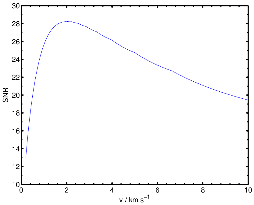
What is the effect of the spacecraft velocity on the SNRs presented in the previous Section? The question is relevant as it can assist the strategy in designing flyby trajectories. Here we show that in practice all that matters is the trajectory location (impact parameter and possibly angle). Within the range of realistic speeds, the SNRs do not vary substantially. The good news is that due to a remarkable coincidence, these speeds are already near optimal.
As Eq. (18) shows, the spacecraft velocity is the conversion factor between the spatial scale of the tidal stress and the time scale at which the instrument measures them. Of course, in detail, this has an effect on expected SNRs. Higher/lower speeds mean a faster/slower scanning of these spatial features, and thus a shift of the template to higher/lower frequencies, whilst keeping the noise ASD fixed. Therefore the SNR has to change. This is shown in Fig. 5, for km and a baseline noise of .
We see that the SNR has a peak at . However this peak is very broad with respect to the type of variations that might be expected from different trajectories leading from L1 to the saddle [14]. For the rough range the SNR varies in the range 27-28, approximately. For (which is pushing it, in terms of real orbits) the variations would be in the approximate range 25-28. The message is clear: get as close to the saddle as possible, never mind the speed. The speed will never be very far off the optimal.
This result can be understood qualitatively. As a crude estimate, anything moving in the Earth-Moon system has a typical speed of the order of 1 km s-1. The MONDian tidal stress for the Earth-Sun saddle displays variations on a length scale of the order of . Therefore the MONDian signal will always be felt by LPF on a time scale of minutes, i.e. in the mHz range. This is just where the instrument noise is lowest, a remarkable coincidence considering that the instrument was built to these specifications for entirely different reasons (astrophysically motivated gravitational wave templates have these time scales). And yet the typical speeds and length scales of the problem combine to make the instrument already optimal for a MONDian saddle test.
IV.2 Improved noise models

A number of improvements to the noise model used in the previous Section are possible. These are the subject of a paper in preparation [28]. Obviously there isn’t a frequency region with white noise. Instead, the noise is likely to be higher than modeled in Section III at high frequencies but lower than expected at low frequencies. The turnover between the two regimes is smooth, as depicted in Figure 6, where we superimposed the simplified noise model used in Section III with the more realistic estimates for ASD for a best and worst case scenario. It has been argued that the worst case scenario might be too pessimistic and the best case scenario too optimistic, so we should take these two models as extremes.
In Figure 7 we plot the SNR as a function of impact parameter with , assuming the two extreme scenarios. As we can see, in the best case scenario we’d need to miss the saddle by more than for the SNR to drop below 5. In the worst case noise scenario, however, that figure would shrink to about . For the currently expected the SNR would be in the range . In spite of the uncertainties, all scenarios lead to optimistic prospects (and even overkill) regarding a detection. We stress that we will know what the noise is, in situ and while on L1. Our forecasts are useful, but we should highlight that they’d become concrete, fixed numbers once the mission goes ahead.

We should add that even if the noise ASD is known, further issues complicate the simple data analysis procedures presented in the previous Section. Most notably the real noise is non-Gaussian and non-stationary. This may increase the probability of a “false alarm”, to use the jargon of gravitational wave detection. Putting a realistic figure to the probability of a false detection requires having the instrument switched on before and after a saddle flyby, characterizing the noise in situ, and evaluating the false alarm rates with real noise. No prior modeling can be a substitute for this. Nonetheless more realistic simulations of the instrument response and noise are possible. We are currently working on these.
The issue of false alarm rates is obviously central should there be detection. But even just planning the experiment, it raises important questions, e.g.: given these rates, is it better to sacrifice at the expense of multiple flybys, or should we put all our efforts into a single flyby with a as low as possible? Should the noise be approximately Gaussian and stationary, the probability of a false detection is simply [15]:
| (20) |
where is the optimal SNR, and is the number of trials. In gravitational wave detection , where is the total observation time and the useful duration of the filtered template. The factor can be very large, so that even substantial SNRs (say 8 or 9) can produce non-negligible rates . In gravitational wave detection this nuisance can be mitigated by coincident observations. We stress that no such problem is present here. We do know where the saddle is for all practical purposes, so , removing the extra factor enhancing the false alarm rate.
The high SNRs we’ve obtained at low suggest that it would not be advisable to sacrifice for the sake of multiple flybys, in order to reduce false alarm rate. This statement should be further scrutinized using real noise. But even if it’s true there is an important sociological element. The reliability of any scientific claim rests on reproducibility. Should there be a positive detection, more than one flyby would go some way towards establishing the case for reproducibility.
IV.3 The Newtonian background and self-gravity

We finish this section by examining two possible systematics that could plague a saddle test: the Newtonian background and the spacecraft self-gravity. These are natural concerns, but their impact is negligible. In establishing this fact it is important not to confuse force and tidal stress. It is also essential to examine the Fourier components of the stress signal and distinguish a DC component from a signal peaking at frequencies to which the experiment is sensitive.
The MONDian saddle signal has a spatial scale . In this region, apart from an inner bubble a few meters across, the Newtonian force is always much larger than the MOND force and also the MONDian acceleration . We recall the discussion in Section II, where we noted that LPF would probe the regime , with . Indeed around , the Newtonian acceleration is . The Newtonian tidal stress is therefore dominant in this regime (with an intensity of the order ), but, crucially, it is approximately a DC component [11, 13]. This is to be contrasted with the distinctively varying MONDian signal (see Fig. 2) which, as we’ve shown, translates into a signal peaking at frequencies where the noise is low. A DC component, on the other hand, is well buried in the noise. It is true that in detail the Newtonian tidal stress is not exactly constant on the scale of . But we do know what it is, to the same accuracy as we know the saddle location and trajectory, and can subtract it off. Furthermore its spectral shape away from its DC component is very different from that predicted by the MOND signal, as shown in Fig. 8. The Newtonian background amounts to the subtraction of a known component.


A related matter was flagged in Section III, and relates to subtracting off from its effect on the renormalization of the gravitational constant. Some of contributes to the Newtonian background and should not be included in the MONDian predictions (cf. Eqn. (13); see also [13]). In Figure 9 we plotted the power spectrum of the non-DC component of the Newtonian tidal stress produced by . The impact of not subtracting the component of contributing to the Newtonian measurement can be appreciated in Figure 9. This figure also gives us an idea of the level of impact an imperfect Newtonian subtraction might have. We considered the transverse tidal stresses felt in trajectories with impact parameters . In the top we subtracted only the DC component, in the bottom we subtracted the full contribution of to the Newtonian tidal stresses. As we can see an imperfect subtraction would produce a spurious ramp in the stresses.
Another issue is LPF’s self-gravity. The mission requirement is that the differential acceleration of the two LPF test masses should be balanced at the level of , but actual performance may beat the nominal requirement by a factor of 10. Yet again this is a DC component and does not affect the measurement in tidal stresses with the distinctive temporal variations we have posited. There are of course time-varying uncertainties in the self-gravity balancing but these are much smaller. They are mainly due to thermoelastic effects, and are on the level of at least down to 1mHz.
An issue related to this concerns the position of the saddle. Naively one might think that with a self-gravity of the order of the position of the saddle would be perturbed by the spacecraft. The two test masses could even generate distinct saddle points due to their gravity. This concern ignores the fact that with realistic impact parameters we are not testing the regime , but the regime with much larger Newtonian accelerations. For instance for an impact parameter of 40 Km we have . Around the Newtonian acceleration is . We’d need to approach the saddle much closer than about meters before self-gravity becomes an issue and the spacecraft itself had to be included in the computation of the location of the saddle.
V MONDian free-functions
In the second part of this paper we examine the generality of our predictions. So far we have focused on type I theories with a specific fitting function (the one used in [13]). But even if we restrict ourselves to type I theories there is a whole free function to play with. Would theorists be able to wriggle out of a negative result availing themselves of this freedom? In the next 3 sections we prove that under general conditions only type I theories with fine-tuned -functions would survive a negative result (with notable exceptions to the rule, spelled out). This conclusion is also expected to apply to type IIB theories, although we won’t prove it in detail. Type III and type IIA theories turn out to be the only ones to evade a LPF saddle test.
In this Section we start by reviewing previously proposed , laying down a common notation. We then discuss criteria for physically permissible , showing that for single power-laws they all produce SNRs of the same order, for impact parameters smaller than 400 km. In Section VI we will then consider more structured functions , with more regimes and scales.
V.1 Notation and previous proposals
As explained in Section II, for type I theories two potentials act on non-relativistic test masses: the Newtonian potential and a fifth force . Thus, the total potential is , or in terms of forces, (as before, we set for simplicity.). We recall that both contributions satisfy Poisson type equations:
| (21) |
| (22) |
where, as before, we write with argument . In the Newtonian limit , whereas MONDian behaviour in is triggered when . Note that here
| (23) |
where is the variable employed by Bekenstein in his original paper on TeVeS [7]. Much confusion has arisen from different notations in this respect.
We should not confuse with the function used in type III theories (cf. Eqn. (7)) and also favoured by astronomers. Even in type I (and also II) theories, we can loosely define an effective , obtained from adding equations (21) and (22) and comparing with Eq. (7). This effective function is frequently used in fits to galactic phenomenology. However the two functions and can only be easily related if the MONDian curl term can be neglected. This proviso is often incorrectly ignored. If the curl term is non-negligible, then type I theories don’t properly have a function, and there’s no substitute for integrating the equations on a case by case basis.
If the curl field can indeed be ignored in the integration of (22), then it’s easy to relate functions and (see, e.g. [8]). Using (21) and (22), their definitions can then be rewritten as and , so that implies:
| (24) |
In addition we can write the argument in terms of by deriving:
| (25) |
Eqns. (24) and (25) provide a parametric expression for . Note that Eq. (24) trivially implies that in the Newtonian regime () MOND has the effect of renormalizing as:
| (26) |
a result already presented in Section II.
Several functions have been previously proposed. The “toy” model used in Bekenstein’s original paper [7] follows from the implicit expression:
| (27) |
A variation was employed in [11] to facilitate analytical work on the 2-body problem:
| (28) |
In some manipulations an inversion of the latter is useful:
| (29) |
A proposal quite distinct from these two can be found in [16]:
| (30) |
with the case first suggested in [21]. To bridge our notation with the used in [16] we should use the dictionary (obtained from direct comparison of (21) and (22) and their counterparts in [16]):
| (31) | |||||
| (32) |
We stress that this function diverges, a property that sets it apart from all those functions which tend to a constant as . Underlying this statement is the postulate that the domain of the function should be excised after the divergence is reached, i.e. one should impose . The distinction between bounded and divergent was extensively studied in [17] and is indeed central to the discussion55 5 As a notational word of caution note that for convergent free-functions we have defined such that as ; whereas in [17] one has , so that in effect we get the dictionary .. A hybrid possibility, incorporating the behaviour of (30) on galactic scales into a bounded function, can be adapted from the proposal in [21], and will be examined in Section VI.1.
There is some debate over which functions best fit astrophysical data. Examples include [29]:
| (33) |
and
| (34) |
| (35) |
With the proviso spelled out above (non-invertibility of a in terms of a in the presence of a curl field), function (35) can be derived from (30). Likewise (27) and (28) lead to:
| (36) | |||||
where we have written three algebraically equivalent expressions to facilitate comparison with the literature. Note that although (36) follows from (35) for , the same doesn’t happen with their functions, and Bekenstein’s proposal (27) is strictly not covered by (30). The claim has been made [21, 17] that galactic observations favour 66 6 As a further notational word of caution (c.f. [17]) note that our tends to (or in the notation of [17], to ). The Milgrom-like proposals considered above all tend to 1. Thus, these proposals can only be approximately true with . Otherwise, the proposals considered here should strictly speaking be labelled , with ..
V.2 Permissible, non-fine tuned functions
Putting aside detailed predictions for galaxy rotation curves (which may well have been combined with inconsistent approximations, e.g. regarding the curl field), the following criteria are reasonable for physically permissible, non-fine tuned functions defining type I theories:
- •
A. The cosmologically measured cannot differ significantly from that measured, say, by the Cavendish experiment. That is: .
- •
B. When the total Newtonian acceleration drops below the full potential must be in the MONDian regime, that is, we need to be in the MONDian regime and to dominate .
- •
C. Function should only have one scale, below which is MONDian, and above which it is near Newtonian. The detailed form of the transition is left undefined, but should have a single transition from to .
Items A and B have already been discussed in Section II. Item B is the most basic requirement for the theory to be of astrophysical use, regardless of the details. Item C has been spelled out because it will be broken in the next Section, to illustrate just how finely tuned would have to be to evade a negative saddle result.
As explained in Section II, these requirements imply that must enter the MONDian regime at a much higher acceleration than , leading to an intermediate regime where is fully MONDian but still sub-dominant to . This implies that for any satisfying these constraints, when (i.e. for astrophysical applications) we must necessarily have
| (37) |
This statement is independent of and only relies on the fact that in the MONDian regime. If the curl term can be ignored we therefore have , and thus (37) follows. Recalling we must conclude that:
| (38) |
The exception to this rule is obtained with a divergent , as already announced in Section II. Then, we discover the interesting behaviour [16, 17] that goes to a constant as grows to infinity, instead of becoming proportional to (c.f. Eq.(9)). Specifically, taking model (30), we find that:
| (39) |
so that asymptotically no renormalization of takes place: . Such a functions would lead to a different , as we’ve seen. In Section VI.1 we’ll show that the MONDian behaviour driven by these functions would be rendered invisible to LPF.
V.3 SNRs and dependence
If we take the whole class of satisfying requirements I, II and III we conclude that they have the same and consequently the same . Fiddling with therefore doesn’t change the spatial scale of the effect for type I theories (and also for type IIB, but not type IIA or type III theories). The predictions for for are also model independent, since they rely on , for . However the predictions referring to regions with depend on the exact form of the transient from to , because they depend on , not . For example,
| (40) |
has a very different fall off from
| (41) |
a point recognized in [11]. Missing the saddle by a lot more than would therefore leave us at the mercy of model dependence, and functions satisfying A, B, C could be found bypassing a negative result, e.g.
| (42) |
with a large . However, for trajectories hitting the region (i.e. for ) the peak of the signal is actually model independent, and therefore the SNRs predicted aren’t expected to depend on the details of the theory.

As an extreme illustration of the model (in)dependence of our SNR predictions we have excised the signal outside the MOND bubble from our templates, imposing an exponential fall off. Fig. 10 is the resulting counterpart to Fig. 4. We see that for our conclusions remain substantially the same. For the SNRs drop much more sharply. This is the worst that can be expected.
Impact parameters around are now considered within easy reach. In order to bypass a negative result we would therefore have to shrink the bubble size, defined by scale . This requires breaking condition C and consider contrived functions with two scales, which we now proceed to do in order to appreciate the full implication of a negative result.
VI A null result and designer functions
It is often difficult to falsify a theory containing free parameters: all that can be readily done is to constrain its parameters. However the constraints may be such that the theory becomes contrived beyond “reasonable”. In what follows we imagine a scenario where no anomalies are found with respect to the Newtonian expectation, for . Obviously all the theories considered so far would be ruled out, to a degree of significance of the same order as their expected SNR. The issue would then become to determine which “designer” functions predict a SNR of order 1, thereby surviving a “no anomaly” result. The more contrived the required , the more blatantly one should throw in the towel.
In proposing a designer we shall impose that it satisfies requirements A and B to the same extent as the functions we’ve been considering. The theory should still be of astrophysical use and not conflict with observations on very general grounds. However, we drop requirement C, allowing the function to have two independent scales (notice that is not independent for the models considered so far). Specifically, we endow with an intermediate power linking the Newtonian regime, where , and the astrophysically relevant MONDian regime, where .

Requirement B demands that for , as before, so that when , and for . Requirement A imposes for large , so that is the same as for the single power-law considered before (cf. Eqn. (26)). If we are to shrink the size of the MOND bubble so as to accommodate a negative outcome from a saddle test, then we need a sharper power, , bridging these two regimes. Thus could increase faster, with decreasing , from its small value in the Newtonian regime, to 1 at . This would reduce and thus . The point is illustrated in Fig. (11), where we have replotted Fig. 1 (made for a with a single power-law; recall the argument in Section II).
These considerations fully specify the function , up to details on the transition regions. We should have:
| (43) | |||||
| (44) | |||||
| (45) |
where the point where non-Newtonian behaviour in is triggered can be interchangeably pinpointed by:
| (46) | |||||
| (47) | |||||
| (48) |
Notice that is a now a truly independent parameter of the theory (which can be traded for ). We still have that when the field dominates as per requirement B, but now the intermediate region, where hasn’t yet dominated but is already non-Newtonian, is in a narrower band of accelerations . As a result the MOND bubble shrinks according to
| (49) |
In Figure 12 we have plotted this dependence. As can be seen, it’s easy to change by an order of magnitude with not much different from 2. To reduce by more than that, however, a very extreme intermediate power would be required77 7 Notice that with this particular model the MOND bubble can never shrink smaller than ..


Regrettably we can never make a model independent statement on what is needed for a SNR of order 1. If nothing is observed then by the nature of the problem we must be making observations in the regime . Therefore we are necessarily probing the transient from to , dependent on the exact form of the function . Nonetheless it is interesting to perform this exercise, assuming a specific function, say:
| (50) |
For this can be expanded as:
| (51) |
Also for the curl field is negligible, so we can write:
| (52) |
and solve it perturbatively. Expanding as in , we have to zero order . To first order we then obtain:
| (53) |
from which the tidal stresses can be inferred.
The results are condensed in Fig. 13, depicting the value of needed for a given and noise level in order for a SNR of one to be obtained (and so a negative result be acceptable). As we can see as soon as we plunge deep into the MOND bubble, a rather unnatural designer becomes necessary to accommodate a negative result.
VI.1 Motivated functions with features
In this paper we have attempted not to mix galaxy rotation fits with our considerations. The reason is that it’s not clear how these fits would stand if performed together with the need to fit Solar system data and a saddle test: the performance of goodness of fit statistics under joint constraints might be very different. Also penalization for extra parameters (such as ) has probably not been properly enforced (see [30] for an example of the implications), and it would certainly behave very differently in a joint fit, where the number of degrees of freedom would be much larger (c.f. the behaviour of the Bayesian information criterion as seen in [30]). Having said this, it may well be that what we labeled “two-scale” or “designer” models is precisely what is needed for one such joint fit. We therefore examine how these motivated functions fare in terms of SNR for a saddle test.
One type of function which evades a saddle test are those which diverge (eg. [16]). As explained before, then the asymptotic is not renormalized, since tends to a constant,
| (54) |
as . Thus the profile of is actually not “designer” in the sense we have been using the word, since it merely changes from one power-law () to another (), never leveling off into a constant. The counterpart of Fig. 1 for this model is plotted in Fig. 14, curve labelled . Since never levels off, , with . A detailed analysis of the saddle effects of this theory cannot be carried out with the methods proposed in this Section. Since doesn’t go to a constant, strictly speaking full MOND-like effects are present for all accelerations, and the curl field can never be neglected. Still, one may expect the order of magnitude of the predicted effects to be small, and the associated saddle bubble to be invisible for LPF. We defer to a future publication a more detailed examination of the predictions associated with these functions.

Divergent functions, however, may fall foul of Solar system constraints (see discussions in [18, 17, 19, 20], but we stress that this conclusion might not be fully general). A compromise can be struck by combining the functional form of the proposed unbounded with a curve flattening to a constant beyond the scales probed by galaxy rotation curves. With such constructions we are plainly entering the realm of the “designer” (or multiple functional form) functions, as defined in this Section. Such multiple regime, multi-scale, functions are implemented in one way or another, in all such proposals [21, 22, 23, 24]. For example, translating [21] into our variables leads to:
| (55) |
On galactic scales this reduces to (30), yet for the purpose of the Solar system we have:
| (56) |
The profile for these models is plotted in Fig. 14, which should be compared to the “natural” Fig. 1 and the more contrived toy model depicted in Fig. 11. These models can be constrained using the methods proposed in this Section. In the face of a negative result, as above, we’d be able to assume we are in the quasi-Newtonian regime, to conclude, after a similar argument, the counterpart of (53):
| (57) |
We can now constrain parameter as before, with the result plotted in Fig. 15. As in Fig. 13 we have plotted the value of (not to be confused with the parameter used there) for which the SNR turns out 1, for a given noise and impact parameter. A negative result from LPF would therefore require to be smaller than this value, which is therefore an upper bound.

VII Conclusions
In this paper we showed how a LPF saddle flyby would either detect MOND to a high SNR or rule it out, if not comprehensively, at least to a large extent. The former conclusion could be expected. Even though in Sections III and IV we provided rigorous and quantitative SNR estimates, the high levels forecast can be understood with a “back of the envelope” calculation. The exercise highlights an uncanny coincidence. The accelerometer aboard LPF has a non-white noise profile, dipping in the region of the mHz, i.e. in the rough time scale of minutes. The motivation for this design lies in the gravitational wave signals to be targeted by LISA. It just so happens that the MONDian bubbles of anomalous tidal stresses around the Earth-Sun-Moon saddles have a length scale of the order of a hundred kilometers. Anything free-falling in the Earth-Moon region has a typical speed of the order of 1km/s. Thus, the time scale for crossing a MONDian bubble will be of the order of minutes: just where the instrument performance is optimal. This is a remarkable coincidence. Scribbling on the back of an envelope, using the expression for the SNR of a noise-matched filter and the order of magnitude of the stresses and noise, promptly reveals double figure SNRs.
The question then arises as to how generic this conclusion is, or conversely, should a negative result be found, how thoroughly have we ruled out MOND. In Section II we scanned the full array of MONDian theories, showing that in the non-relativistic regime they fall into only 3 categories (which we labelled type I, IIA/B and III). Even if we restrict ourselves to type I theories (a class containing the vast majority of these theories, including TeVeS), we benefit from the leverage of a free function, . Could MONDologists use to survive a negative result?
In Sections V we examined functions on offer in the literature and laid down criteria for reasonable based on astrophysical usefulness, viability in the face of constraints, and naturalness. We found that once these criteria are taken into account the size of the MOND bubble, , is fixed. There are exceptions to this rule; e.g. diverging functions, but these may be subject to other constraints (they will be examined elsewhere). Predictions for what happens inside the bubble are also model independent; however the tidal stress anomalies outside the bubble depend on the transient from MONDian into Newtonian regime, with a fall-off which is indeed model dependent. Thus, for impact parameters smaller than the predicted SNRs are robust, and do not change substantially with the model. For the currently expected (around , with ) this is indeed the case.
Therefore the only way for MOND to wriggle out of a negative LPF result would be to change the bubble size . This can only be accomplished with “designer” -functions. If is allowed to have two scales and two power-laws away from its Newtonian value of 1, then it is possible to bypass a negative LPF result. Even for undemanding noise levels and impact parameters, the intermediate power becomes very contrived. Similarly fine-tuned functions have been proposed in the literature. In Section VI.1, we showed how LPF could be used to constrain them. The point remains that one would have to bend backwards to accommodate a negative result, within type I theories. There are exceptions to this rule (for example diverging functions) and these derserve further attention.
Although we didn’t present quantitative results for type II theories, the same conclusions apply qualitatively to type IIB theories (but not type IIA theories). If is renormalized and the free function is chosen to produce the same phenomenology as type I theories (in particular with regards to and MONDian behaviour), then the MOND bubble has the same size, and the anomalous tidal stresses are of the same order. As explained in Section II, in both types of theory MONDian behaviour is due to an extra field , and if one attends simultaneously to and for , then MONDian behavior in should be triggered at the same Newtonian acceleration . This implies a MONDian bubble of the same size . Furthermore the (also -independent) effects inside the bubble are different from type I predictions, but stronger. Type II theories don’t have a curl field (in the sense define above), a feature which softens the anomalous tidal stresses in type I theories [11]. A detailed quantitative prediction for type II theories is currently being investigated (see [26]; also we reference here a paper on the matter which has appeared since the present paper was submitted [31].)
However, it may be that the relativistic mother theory is set up in such a way that the cosmological and non-relativistic coincide, the case of type IIA theories. In this case the MOND bubble around the saddle is very small. Likewise type III theories (or, rather, its single relativistic realization, the Einstein-Aether theory) produce effects around saddles which are unobservable with current technology. In these theories is not renormalized and , so that the MOND bubble is a few meters across. Remarkably, solar system tests are extremely constraining upon type III theories, due to the so-called external field effect [9]. By contrast solar system effects for type I and IIB theories are suppressed by a factor of . Thus saddle tests and planetary orbits seem to be complementary in constraining MONDian theories.
We close by noting that we could, of course, detach our considerations entirely from the MOND paradigm (as an alternative to dark matter), and regard these theories formally as a class on alternative theories of gravity (see [32] for an extensive review). It is remarkable that only three classes of theories emerge in the non-relativistic regime, which we labelled type I, II and III in Section II. We could then view and as free parameters, converting a LPF saddle flyby into a constraint or a detection in this space. We are currently working on this alternative approach.
Acknowledgements.
We’d like to thank Luc Blanchet, Tim Clifton, Benoit Famaey, Pedro Ferreira, Martin Hewitson, Natalia Korsakova, Mordehai Milgrom, B.S. Sathyaprakash, Christian Trenkle and an anonymous referee for comments and suggestions. We’re also grateful for the input from the whole LPF science team, provided at two meetings at RAL and IC. Our numerical work was performed on the COSMOS supercomputer, which is supported by STFC, HEFCE and SGI.References
- [1] M. Milgrom, Astrophys. J. 270, 365 (1983).
- [2] R. H. Sanders, Mon. Not. Roy. Astron. Soc. 363, 459 (2005), eprint astro-ph/0502222.
- [3] T. G. Zlosnik, P. G. Ferreira, and G. D. Starkman, Phys. Rev. D74, 044037 (2006), eprint gr-qc/0606039.
- [4] T. G. Zlosnik, P. G. Ferreira, and G. D. Starkman, Phys. Rev. D75, 044017 (2007), eprint astro-ph/0607411.
- [5] M. Milgrom, Phys. Rev. D80, 123536 (2009a), eprint 0912.0790.
- [6] M. Milgrom, Mon. Not. Roy. Astron. Soc. 405, 1129 (2010), eprint 1001.4444.
- [7] J. D. Bekenstein, Phys. Rev. D70, 083509 (2004); Erratum-ibid. D71, 069901 (2005), eprint astro-ph/0403694.
- [8] C. Skordis, Class. Quant. Grav. 26, 143001 (2009), eprint 0903.3602.
- [9] L. Blanchet and J. Novak (2011), eprint 1105.5815.
- [10] M. Milgrom (2009b), eprint 0906.4817.
- [11] J. Bekenstein and J. Magueijo, Phys. Rev. D73, 103513 (2006), eprint astro-ph/0602266.
- [12] P. McNamara, S. Vitale, and K. Danzmann (LISA), Class. Quant. Grav. 25, 114034 (2008).
- [13] N. Bevis, J. Magueijo, C. Trenkel, and S. Kemble, Class. Quant. Grav. 27, 215014 (2010), eprint 0912.0710.
- [14] C. Trenkel, S. Kemble, N. Bevis, and J. Magueijo, submitted (2009).
- [15] B. S. Sathyaprakash and B. F. Schutz, Living Rev. Rel. 12, 2 (2009), eprint 0903.0338.
- [16] G. W. Angus, B. Famaey, and H. Zhao, Mon. Not. Roy. Astron. Soc. 371, 138 (2006), eprint astro-ph/0606216.
- [17] B. Famaey, G. Gentile, J.-P. Bruneton, and H.-S. Zhao, Phys. Rev. D75, 063002 (2007), eprint astro-ph/0611132.
- [18] B. Famaey and S. McGaugh, Living Reviews in Relativity, in preparation (2011).
- [19] R. Sanders, Mon.Not.Roy.Astron.Soc. 370, 1519 (2006), eprint astro-ph/0602161.
- [20] G. Gentile, B. Famaey, and W. de Blok, Astron.Astrophys. 527, A76 (2011), eprint 1011.4148.
- [21] H.-S. Zhao and B. Famaey, Astrophys. J. 638, L9 (2006), eprint astro-ph/0512425.
- [22] J.-P. Bruneton and G. Esposito-Farese, Phys.Rev. D76, 124012 (2007), eprint 0705.4043.
- [23] S. McGaugh, Astrophys.J. 683, 137 (2008).
- [24] H. Zhao, J.Phys.Conf.Ser. 140, 012002 (2008).
- [25] J. Bekenstein and M. Milgrom, Astrophys. J. 286, 7 (1984).
- [26] A. Mozaffari (2011), arXiv:1112.5443.
- [27] C. Helstrom (1968), Statistical Theory of Signal Detection, Pergamon Press, Oxford; New York.
- [28] C. Trenkle et al (2011), in preparation.
- [29] B. Famaey and J. Binney, Mon. Not. Roy. Astron. Soc. 363, 603 (2005), eprint astro-ph/0506723.
- [30] J. Magueijo and R. D. Sorkin, Mon.Not.Roy.Astron.Soc. 377, L39 (2007), eprint astro-ph/0604410.
- [31] P. Galianni, M. Feix, H. Zhao, and K. Horne (2011), eprint 1111.6681.
- [32] T. Clifton, P. G. Ferreira, A. Padilla, and C. Skordis (2011), eprint 1106.2476.