Abstract — We present an update of the Standard Model fit to electroweak precision data. We include newest experimental results on the top quark mass, the $W$ mass and width, and the Higgs boson mass bounds from LEP, Tevatron and the LHC. We also include a new determination of the electromagnetic coupling strength at the $Z$ pole. We find for the Higgs boson mass $91^{\>+30}_{\>-23}\>\mathrm{Ge\kern-0.92505ptV}$ and $120^{\>+12}_{\>-5}\>\mathrm{Ge\kern-0.92505ptV}$ when not including and including the direct Higgs searches, respectively. From the latter fit we indirectly determine the $W$ mass to be $(80.360^{+0.014}_{-0.013})\>\mathrm{Ge\kern-0.92505ptV}$ . We exploit the data to determine experimental constraints on the oblique vacuum polarisation parameters, and confront these with predictions from the Standard Model (SM) and selected SM extensions. By fitting the oblique parameters to the electroweak data we derive allowed regions in the BSM parameter spaces. We revisit and consistently update these constraints for a fourth fermion generation, two Higgs doublet, inert Higgs and littlest Higgs models, models with large, universal or warped extra dimensions and technicolour. In most of the models studied a heavy Higgs boson can be made compatible with the electroweak precision data.

1 Introduction

By exploiting contributions from radiative corrections, precision measurements, in line with accurate theoretical predictions, can be used to probe physics at higher energy scales than the masses of the particles directly involved in the experimental reactions. Theory and experimental data are confronted and unknown model parameters are constrained by means of multi-parameter fits. For cases where the parameter space is overconstrained it is possible to derive p-values for the compatibility between data and theoretical model [1], and hence to directly assess the validity of the model. Such an approach has been used in the Gfitter analysis of the Standard Model (SM) in light of the electroweak precision data [2], which we revisit in this paper with updated experimental constraints. Global electroweak SM fits are also routinely performed by the LEP Electroweak Working Group [3] and for the electroweak review of the Particle Data Group [4].

Assuming that the dominant virtual contributions to the electroweak observables arise through vacuum polarisation loops, and that other corrections, such as vertex diagrams involving light quarks, or box and bremsstrahlung diagrams, are scale suppressed, physics beyond the SM (BSM) can be parametrised through so-called quantum oblique corrections, for which several parametrisations exist in the literature [5, 6, 7, 8, 9, 10, 11, 12, 13]. A popular choice are the $S,T$ and $U$ parameters [5, 6], which have been computed for most of the prevailing BSM models. The $S,\,T,\,U$ parameters are defined with respect to a canonical SM reference so that, for SM parameters identical to the reference point values, the parameters vanish in the SM. In that case, any significant non-zero value in at least one parameter would hint at BSM physics.

In this paper we derive, for a chosen SM reference point, experimental constraints on the $S,\,T,\,U$ parameters, and compare them with predictions from the SM and various BSM models. We study a fourth fermion generation, two Higgs and inert Higgs doublet models, the littlest Higgs model and models with large, universal and warped extra dimensions as well as technicolour. We also use the experimental constraints to derive allowed regions in the relevant parameter spaces of these models. Several similar analyses have been performed and published in the past. We refer to these in the corresponding BSM sections. The current analysis revisits these works and provides a consistent set of BSM constraints derived from the most recent electroweak data and using the statistics tools of the Gfitter framework [2]. Its modular design allows us to determine these constraints directly in the fit, thus invoking known two-loop and beyond two-loop SM corrections.

The paper is organised as follows. The updated SM fit to the electroweak precision data is discussed in Section 2. An introduction of the oblique parameter formalism is given in Section 3, where we also present the experimental results, and discuss the predictions from the SM. Additional formulas are provided in the Appendix. In Section 4 and subsections we discuss the oblique corrections for the aforementioned BSM models and the corresponding constraints in the relevant parameter spaces.

2 The Global Fit of the Electroweak Standard Model

We present an update of the SM fit to electroweak precision data, the results of which will be used as a reference throughout this paper. A detailed description of the experimental data, the theoretical calculations, and the statistical methods used in the Gfitter analysis is given in our reference paper [2]. Since its publication, the fit software has been continuously maintained and kept in line with the experimental and theoretical progress. Here, we shall recall only the most important aspects of the fit, outline recent changes, which mainly concern updates of the experimental or phenomenological input data, and present a full result table together with representative plots and a discussion of selected results.

2.1 Fit inputs

Standard Model predictions

The SM predictions for the electroweak precision observables measured by the LEP, SLC, and Tevatron experiments are fully implemented. State-of-the-art calculations are used, in particular the full two-loop and leading beyond-two-loop corrections for the prediction of the $W$ mass and the effective weak mixing angle [14, 15, 16], which exhibit the strongest constraints on the Higgs mass. A modification to Ref. [2] is the usage of accurate parametrisations [17, 18, 19, 20] for the calculation of the vector and axial-vector couplings, $g_{A}^{f}$ and $g_{V}^{f}$ , which are computed at one-loop level and partly at two-loop level for ${\cal O}(\alpha\alpha_{s})$ .¹¹ 1 Up to two-loop electroweak corrections are available in Refs. [21, 22, 23, 24, 25, 26, 27, 28, 29, 30, 31, 32]. All known QCD corrections are given in Refs. [22, 26, 33]. Small additional correction factors, determined from a comparison with the Fortran ZFITTER package [22, 26], are used to accommodate heavy Higgs masses [34]. These couplings enter the calculations of the partial and total widths of the $Z$ and the total width of the $W$ boson, which, due to the insufficient experimental precision, display a weak constraint on the Higgs mass only. In the radiator functions [32, 26] the fourth-order (3NLO) perturbative calculation of the massless QCD Adler function [35] is also included, allowing the fit to determine the strong coupling constant with very small theoretical uncertainty.

The SM parameters relevant for the prediction of the electroweak observables are the coupling constants of the electromagnetic ( $\alpha$ ), weak ( $G_{\scriptscriptstyle F}$ ) and strong interactions ( $\alpha_{\scriptscriptstyle S}$ ), and the masses of the elementary bosons ( $M_{Z}$ , $M_{W}$ , $M_{H}$ ) and fermions ( $m_{f}$ ), where neutrino masses are set to zero. Electroweak unification results in a massless photon and a relation between the electroweak gauge boson masses and couplings, thus reducing the number of unknown SM parameters by two. The SM gauge sector is left with four free parameters taken to be $\alpha$ , $M_{Z}$ , $G_{\scriptscriptstyle F}$ and $\alpha_{\scriptscriptstyle S}$ . Simplification of the fit is achieved by fixing parameters with insignificant uncertainties compared to the sensitivity of the fit. The final list of floating fit parameters is: $M_{Z}$ , $M_{H}$ , $m_{t}$ , $\overline{m}_{b}$ , $\overline{m}_{c}$ ,²² 2 In the analysis and throughout this paper we use the $\overline{\rm MS}$ renormalised masses of the $c$ and $b$ quarks, $\overline{m}_{c}(\overline{m}_{c})$ and $\overline{m}_{b}(\overline{m}_{b})$ , at their proper scales. In the following they are denoted with $\overline{m}_{c}$ and $\overline{m}_{b}$ respectively, and their values are taken from [36]. $\Delta\alpha_{\rm had}^{(5)}(M_{Z}^{2})$ and $\alpha_{\scriptscriptstyle S}(M_{Z}^{2})$ , where only the latter parameter is kept fully unconstrained allowing an independent measurement.³³ 3 Using an external precision measurement of $\alpha_{\scriptscriptstyle S}(M_{Z}^{2})$ in the fit has been studied in Ref. [2] and found to have a negligible impact on the $M_{H}$ result.

Theoretical uncertainties due to unknown higher order terms affecting the predictions of $M_{W}$ and $\sin\!^{2}\theta^{\ell}_{{\rm eff}}$ [14, 16] are parametrised by $\delta_{\rm th}M_{W}\simeq 4\>\mathrm{Me\kern-1.00006ptV}$ and $\delta_{\rm th}\sin\!^{2}\theta^{\ell}_{{\rm eff}}\simeq 4.7\cdot 10^{-5}$ . They are treated according to the Rfit scheme [37, 38] as freely varying but bound parameters in the fit.

Experimental input

The experimental results used in the fit include the electroweak precision data measured at the $Z$ pole [39] ( $Z$ resonance parameters, partial $Z$ cross sections, neutral current couplings⁴⁴ 4 We do not include the CDF and D0 measurements of the forward-backward charge asymmetry in $p\overline{p}\to Z/\gamma^{\star}+X\to e^{+}e^{-}+X$ events, used to extract the $\sin\!^{2}\theta^{e}_{{\rm eff}}$ values $0.2238\pm 0.0040\pm 0.0030$ by CDF [40], and $0.2326\pm 0.0018\pm 0.0006$ by D0 [41], as their impact so far is negligible compared to the precision of the combined $Z$ pole data in the fit, $\sin\!^{2}\theta^{\ell}_{{\rm eff}}=0.23143\pm 0.00013$ . Also due to lack of precision, we do not include results from atomic parity violation measurements, and from parity violation left-right asymmetry measurements using fixed target polarised Møller scattering at low $Q^{2}$ (see [2] for references). The NuTeV Collaboration measured ratios of neutral and charged current cross sections in neutrino-nucleon scattering at an average $Q^{2}\simeq 20\mathrm{Ge\kern-1.00006ptV}^{2}$ using both muon neutrino and muon anti-neutrino beams [42]. The results derived for the effective weak couplings are not included in this analysis because of unclear theoretical uncertainties from QCD effects such as next-to-leading order corrections and nuclear effects of the bound nucleon parton distribution functions [43] (for reviews see, e.g., Refs. [44, 45]). ), their experimental correlations [39], and the latest $W$ mass world average $M_{W}=80.399\pm 0.023\>\mathrm{Ge\kern-1.00006ptV}$ [46] and width $\Gamma_{W}=2.098\pm 0.048\>\mathrm{Ge\kern-1.00006ptV}$ [47].

Furthermore we use the newest average of the direct Tevatron top mass measurements $m_{t}=173.3\pm 0.9\pm 0.6\>\mathrm{Ge\kern-1.00006ptV}$ [48], which is interpreted in terms of a pole mass. It should be noted that the theoretical uncertainties arising from nonperturbative colour-reconnection effects in the fragmentation process [49, 50], and from ambiguities in the top-mass definition [51, 52], affect the (kinematic) top mass measurement. Their quantitative estimate is difficult and may reach roughly 0.5 $\mathrm{Ge\kern-1.00006ptV}$ each, where the systematic error due to shower effects could be larger [49]. Especially the colour-reconnection and shower uncertainties, estimated by means of a toy model, need to be verified with experimental data and should be included in the top mass result and uncertainty published by the experiments. None of these additional theoretical uncertainties on $m_{t}$ is included in the fit.

The top mass definition entering the SM $p\overline{p}\to t\overline{t}+X$ inclusive cross section prediction is unambiguous once a renormalisation procedure is defined and assuming no contributions from new physics to the measured cross section.⁵⁵ 5 In Ref. [53] the $\overline{\rm MS}$ scheme is used to predict the QCD scaling function versus scale ratios (including the dependence on the top mass) that, convolved with the parton luminosity and multiplied by $(\alpha_{\scriptscriptstyle S}/\overline{m}_{t})^{2}$ , determines the inclusive $t\overline{t}$ production cross section. The experimental cross section measurement thus allows one to infer $\overline{m}_{t}$ and hence the pole mass (being the renormalised quark mass in the on-shell renormalisation scheme) from the ratio of the corresponding renormalisation factors known to three loops [54]. The numerical analysis must account for the dependence of the experimental cross section value on the top mass used to determine the detector acceptance and reconstruction efficiencies. The latest extraction of the top mass from the $t\overline{t}$ cross section was performed by the D0 Collaboration. Using a theoretical $\sigma_{t\overline{t}}(m_{t})$ prediction based on approximate NNLO QCD that includes all next-to-next-to-leading logarithms relevant in NNLO QCD [53], the top pole mass, derived from the measured cross section $\sigma_{t\overline{t}}(m_{t}=172.5\>\mathrm{Ge\kern-1.00006ptV})=8.13^{\>+1.02}_{\>-0.90}\>{\rm pb}$ [55], was found to be $m_{t}=167.5^{\>+5.0}_{\>-4.5}\>\mathrm{Ge\kern-1.00006ptV}$ [56].⁶⁶ 6 The quoted error on the extracted top mass does not include the ambiguity in the Monte Carlo top mass interpretation. A similar value for $m_{t}$ is obtained when using the cross section prediction of Ref. [57]. While the nominal electroweak fits in this work use the direct Tevatron top mass average, we will employ the cross section based value for comparison.

For the vacuum polarisation contribution from the five lightest quark flavours to the electromagnetic coupling strength at $M_{Z}$ we use the evaluation $\Delta\alpha_{\rm had}^{(5)}(M_{Z}^{2})=(2757\pm 10)\cdot 10^{-5}$ [58].⁷⁷ 7 A mistake has been found in the published result of $\Delta\alpha_{\rm had}^{(5)}(M_{Z}^{2})$ [58]. The corrected result used here is reported in Version 2 of the arXiv submission [1010.4180]. It includes new $\pi^{+}\pi^{-}$ cross section data from BABAR and KLOE, new multi-hadron data from BABAR, a reestimation of missing low-energy contributions using results on cross sections and process dynamics from BABAR (cf. references in [58]), and a reevaluation of the continuum contribution from perturbative QCD at four loops . Mostly the reevaluation of the missing low-energy contributions has led to a smaller $\Delta\alpha_{\rm had}^{(5)}(M_{Z}^{2})$ estimate compared to that of Ref. [59] used in our previous fits. Reference [58] quotes a functional dependence of the central value of $\Delta\alpha_{\rm had}(M_{Z}^{2})$ on $\alpha_{\scriptscriptstyle S}(M_{Z}^{2})$ of $0.37\cdot 10^{-4}\times(\alpha_{\scriptscriptstyle S}(M_{Z}^{2})-0.1193)/0.0028$ around the given central value of $\Delta\alpha_{\rm had}(M_{Z}^{2})$ . This dependence is included via the rescaling mechanism [2] in the Gfitter software.

Refer to caption — Figure 1: Contribution to the $\chi^{2}$ test statistic versus $M_{H}$ derived from the experimental information on direct Higgs boson searches made available by the LEP Higgs Boson and the Tevatron New Phenomena and Higgs Boson Working Groups [60, 61, 62] and the ATLAS [63] and CMS Collaborations [64]. The solid (black) and dashed (dark red) lines show the contribution from LEP and Tevatron, while the dotted (light red) and dashed-dotted (blue) lines indicate the constraints obtained from the 2010 data by ATLAS and CMS, respectively. Following the original figures they have been interpolated by straight lines for the purpose of presentation and in the fit. The light green area gives the combination of these measurements. Correlations due to common systematic errors have been neglected in this combination. See text for a description of the method applied.

This setup defines the standard electroweak fit.

The complete electroweak fit also includes the information from the direct Higgs searches at LEP [60], Tevatron [61, 62] and – for the first time – the LHC. We include results from the 2010 LHC run published by ATLAS (combining six different final states) [63] and CMS ( $H\to WW\to\ell\nu\ell\nu$ ) [64], where correlations due to common systematic errors between these results are neglected. Because in the electroweak fit we are interested in the compatibility of the SM (assumed to be true) with the data, we transform the one-sided confidence level, ${\rm CL}_{\rm s+b}$ , reported by the experiments,⁸⁸ 8 In lack of published ${\rm CL}_{\rm s+b}$ values by ATLAS [63] we approximate a chi-squared behaviour of the $\tilde{q}_{\mu}$ test statistics used [65] and compute ${\rm CL}_{\rm s+b}\simeq{\rm Prob}(\tilde{q}_{1},1)$ , where the published $p_{0}$ values have been converted into $\tilde{q}_{0}$ , and $\tilde{q}_{1}=\tilde{q}_{0}-2{\rm LLR}$ with the definition ${\rm LLR}=-2\ln({\cal L}(1,\hat{\hat{\theta}})/{\cal L}(0,\hat{\theta}))$ . A nearly identical result is found with ${\rm CL}_{\rm s+b}\simeq{\rm Prob}(-2{\rm LLR}+{\rm offset},1)$ , where the offset of $1.1$ has been added to ensure positive values over the Higgs mass range, and using the published LLR numbers only. These are the numbers used in the fit. into a two-sided confidence level, ${\rm CL}^{\rm 2-sided}_{\rm s+b}$ . This transformation reduces the statistical constraint from the direct Higgs searches compared to that of the one-sided ${\rm CL}_{\rm s+b}$ , because positive fluctuations (or signals), beyond the signal plus background expectation, are penalised by the test statistics as are negative fluctuations (or absence of signals). The contribution to the $\chi^{2}$ test statistic minimised in the fit is obtained from $\delta\chi^{2}(M_{H})=2\cdot[{\rm Erf}^{-1}(1-{\rm CL}^{\rm 2-sided}_{\rm s+b}(M_{H}))]^{2}$ , where we add up the terms from the LEP, Tevatron and LHC experiments ignoring the correlations among these. As the LHC results are statistics dominated this assumption should not be too inaccurate. Nevertheless, an official combination of all the results by the experiments should be encouraged. A more detailed discussion of our combination method is given in Ref. [2]. The resulting $\delta\chi^{2}$ versus $M_{H}$ is shown in Fig. 1 for LEP, Tevatron, ATLAS and CMS individually (lines) as well as their combination (shaded/green area). Note that the minimum $\delta\chi^{2}$ at $M_{H}\sim 125\>\mathrm{Ge\kern-1.00006ptV}$ is not to be interpreted (in a Bayesian sense) as a “most probable Higgs mass”, but as an area where the experimental sensitivity is not sufficient to either exclude nor confirm a Higgs boson.

The second column in Table 1 gives an overview of all the input quantities used in the fit.

2.2 Fit results

The standard and complete fits converge with global minimum values of the test statistics of respectively $\chi^{2}_{{\rm min}}=16.6$ and $\chi^{2}_{{\rm min}}=17.8$ for 13 and 14 degrees of freedom, giving the naive p-values ${\rm Prob}(\chi^{2}_{{\rm min}},13)=0.21$ and ${\rm Prob}(\chi^{2}_{{\rm min}},14)=0.23$ , which have been confirmed by pseudo experiments generated with Monte Carlo techniques.⁹⁹ 9 The ${\rm CL}_{\rm s+b}$ obtained from the direct Higgs searches has been left unaltered during the Monte Carlo based p-value evaluation of the complete fit. This is justified by the strong statistical significance of the LEP constraint, which drives the contribution of the direct Higgs searches to the $\chi^{2}_{{\rm min}}$ . The minor improvement in the p-value of the complete fit with respect to our earlier result [2] arises from the increased best-fit value of the Higgs mass in the standard fit (see below), owing to the reduced electromagnetic coupling strength at $M_{Z}^{2}$ [58]. The new result reduces the tension with the direct Higgs boson searches.

		Results from global EW fits:		Fits w/o exp. input in given line:
Parameter	Input value	Standard fit	Complete fit	Complete fit	$M_{H}\equiv 120$ GeV
$M_{Z}$ [GeV]	$91.1875\pm 0.0021$	$91.1874\pm 0.0021$	$91.1877\pm 0.0021$	$91.1959^{\,+0.0150}_{\,-0.0148}$	$91.1956^{\,+0.0141}_{\,-0.0136}$
$\Gamma_{Z}$ [GeV]	$2.4952\pm 0.0023$	$2.4959\pm 0.0015$	$2.4955\pm 0.0014$	$2.4952\pm 0.0017$	$2.4952\pm 0.0017$
$\sigma_{\rm had}^{0}$ [nb]	$41.540\pm 0.037$	$41.478\pm 0.014$	$41.478\pm 0.014$	$41.469\pm 0.015$	$41.469\pm 0.015$
$R^{0}_{\ell}$	$20.767\pm 0.025$	$20.743\pm 0.018$	$20.741\pm 0.018$	$20.719^{\,+0.025}_{\,-0.028}$	$20.717^{\,+0.027}_{\,-0.026}$
$A_{\rm FB}^{0,\ell}$	$0.0171\pm 0.0010$	$0.01640\pm 0.0002$	$0.01624^{\,+0.0002}_{\,-0.0001}$	$0.01620^{\,+0.0002}_{\,-0.0001}$	$0.01620^{\,+0.0002}_{\,-0.0001}$
$A_{\ell}$ ^(⋆)	$0.1499\pm 0.0018$	$0.1479\pm 0.0010$	$0.1472^{+0.0009}_{-0.0007}$	–	–
$A_{c}$	$0.670\pm 0.027$	$0.6683^{\,+0.00044}_{\,-0.00043}$	$0.6680^{\,+0.00040}_{\,-0.00028}$	$0.6679^{\,+0.00038}_{\,-0.00027}$	$0.6680^{\,+0.00038}_{\,-0.00026}$
$A_{b}$	$0.923\pm 0.020$	$0.93469^{\,+0.00009}_{\,-0.00008}$	$0.93463^{\,+0.00007}_{\,-0.00005}$	$0.93462^{\,+0.00008}_{\,-0.00005}$	$0.93462^{\,+0.00008}_{\,-0.00003}$
$A_{\rm FB}^{0,c}$	$0.0707\pm 0.0035$	$0.0741^{\,+0.0006}_{\,-0.0005}$	$0.0737^{\,+0.0005}_{\,-0.0004}$	$0.0738^{\,+0.0005}_{\,-0.0004}$	$0.0738^{\,+0.0005}_{\,-0.0004}$
$A_{\rm FB}^{0,b}$	$0.0992\pm 0.0016$	$0.1037\pm 0.0007$	$0.1032^{\,+0.0006}_{\,-0.0005}$	$0.1037^{\,+0.0003}_{\,-0.0005}$	$0.1037^{\,+0.0003}_{\,-0.0005}$
$R^{0}_{c}$ [ $10^{-4}$ ]	$1721\pm 30$	$1722.9^{\,+0.7}_{\,-0.6}$	$1722.9\pm 0.6$	$1722.9\pm 0.6$	$1722.9\pm 0.6$
$R^{0}_{b}$ [ $10^{-4}$ ]	$2162.9\pm 6.6$	$2157.6^{\,+0.5}_{\,-0.8}$	$2157.5^{\,+0.5}_{\,-0.8}$	$2157.5^{\,+0.5}_{\,-0.8}$	$2157.5^{\,+0.5}_{\,-0.8}$
$\sin\!^{2}\theta^{\ell}_{{\rm eff}}(Q_{\rm FB})$	$0.2324\pm 0.0012$	$0.23141^{\,+0.00012}_{\,-0.00013}$	$0.23150^{\,+0.00008}_{\,-0.00010}$	$0.23148^{\,+0.00010}_{\,-0.00009}$	$0.23149^{\,+0.00009}_{\,-0.00010}$
$M_{H}$ [GeV] ^(∘)	${\rm CL}_{\rm s+b}$	$91^{+30[+74]}_{-23[-42]}$	$120^{+12[+23]}_{-5[-6]}$	$91^{+30[+74]}_{-23[-42]}$	$120$ (fixed)
$M_{W}$ [GeV]	$80.399\pm 0.023$	$80.383^{\,+0.014}_{\,-0.015}$	$80.370^{\,+0.007}_{\,-0.009}$	$80.360^{\,+0.014}_{\,-0.013}$	$80.359^{\,+0.015}_{\,-0.008}$
$\Gamma_{W}$ [GeV]	$2.085\pm 0.042$	$2.093\pm 0.001$	$2.092\pm 0.001$	$2.092\pm 0.001$	$2.092\pm 0.001$
$\overline{m}_{c}$ [GeV]	$1.27^{\,+0.07}_{\,-0.11}$	$1.27^{\,+0.07}_{\,-0.11}$	$1.27^{\,+0.07}_{\,-0.11}$	–	–
$\overline{m}_{b}$ [GeV]	$4.20^{\,+0.17}_{\,-0.07}$	$4.20^{\,+0.16}_{\,-0.07}$	$4.20^{\,+0.16}_{\,-0.07}$	–	–
$m_{t}$ [GeV]	$173.3\pm 1.1$	$173.4\pm 1.1$	$173.7\pm 1.1$	$177.2\pm 3.4$ ^(▽)	$176.8^{+3.1}_{-3.0}$
$\Delta\alpha_{\rm had}^{(5)}(M_{Z}^{2})$ ^(†△)	$2757\pm 10$	$2758\pm 11$	$2756\pm 11$	$2729^{+57}_{-50}$	$2730^{+57}_{-46}$
$\alpha_{s}(M_{Z}^{2})$	–	$0.1193\pm 0.0028$	$0.1194\pm 0.0028$	$0.1194\pm 0.0028$	$0.1194\pm 0.0028$
$\delta_{\rm th}M_{W}$ [MeV]	$[-4,4]_{\rm theo}$	$4$	$4$	–	–
$\delta_{\rm th}\sin\!^{2}\theta^{\ell}_{{\rm eff}}$ ^(†)	$[-4.7,4.7]_{\rm theo}$	$4.7$	$4.7$	–	–

^(⋆)Average of LEP ( $A_{\ell}=0.1465\pm 0.0033$ ) and SLD ( $A_{\ell}=0.1513\pm 0.0021$ ) measurements. The complete fit w/o the LEP (SLD) measurement gives $A_{\ell}=$ $0.1473^{\,+0.0010}_{\,-0.0006}$ ( $A_{\ell}=$ $0.1469^{\,+0.0007}_{\,-0.0005}$ ). ^(∘)In brackets the $2\sigma$ . ^(†)In units of $10^{-5}$ . ^(△)Rescaled due to $\alpha_{s}$ dependency. ^(▽)Ignoring a second less significant minimum, cf. Fig. 7 and Eq. (6).

Table 1: Input values and fit results for the observables and parameters of the global electroweak fit. The first and second columns list respectively the observables/parameters used in the fit, and their experimental values or phenomenological estimates (see text for references). The subscript “theo” labels theoretical error ranges. Boldface letters indicate that a parameter is floating in the fit. The third (fourth) column quotes the results of the standard (complete) fit not including (including) the constraints from the direct Higgs searches at LEP, Tevatron and the LHC in the fit. In case of floating parameters the fit results are directly given, while for (non-floating) observables the central values and errors are obtained by individual profile likelihood scans. The last two columns give the fit results for each parameter without using the corresponding experimental or phenomenological constraint in the fit (indirect determination), for the complete fit and when assuming the Higgs mass to be known and precisely measured at 120 GeV, respectively.

Parameter	$\ln M_{H}$	$\Delta\alpha_{\rm had}^{(5)}(M_{Z}^{2})$	$M_{Z}$	$\alpha_{\scriptscriptstyle S}(M_{Z}^{2})$	$m_{t}$	$\overline{m}_{c}$	$\overline{m}_{b}$
$\ln M_{H}$	1	$-0.18$	0.13	0.02	0.32	$-0.00$	$-0.01$
$\Delta\alpha_{\rm had}^{(5)}(M_{Z}^{2})$		1	$-0.01$	0.35	$0.00$	0.00	0.01
$M_{Z}$			1	$-0.01$	$-0.01$	$-0.00$	$-0.00$
$\alpha_{\scriptscriptstyle S}(M_{Z}^{2})$				1	0.03	0.01	0.04
$m_{t}$					1	0.00	$-0.00$
$\overline{m}_{c}$						1	0.00

Table 2: Correlation coefficients between the free fit parameters in the standard fit. The correlations with and between the varying theoretical error parameters

\delta_{\rm th}

are negligible in all cases.

The results for the parameters and observables of the two fits are given in columns three and four of Table 1,¹⁰¹⁰ 10 It is noticable that the values of the four theoretical uncertainty parameters converge at the limits of their allowed intervals. This is explained by their uniform contribution to the $\chi^{2}$ function but the necessarily non-uniform values of the global $\chi^{2}$ function that depends on these theory parameters. The fit thus converges at the extrema of the allowed ranges. together with their one standard deviation ( $\sigma$ ) intervals derived from the $\Delta\chi^{2}$ test statistics.¹¹¹¹ 11 We have verified the chi-squared property of the test statistics by sampling pseudo MC experiments. The correlation coefficients are given in Table 2 (for the standard fit).

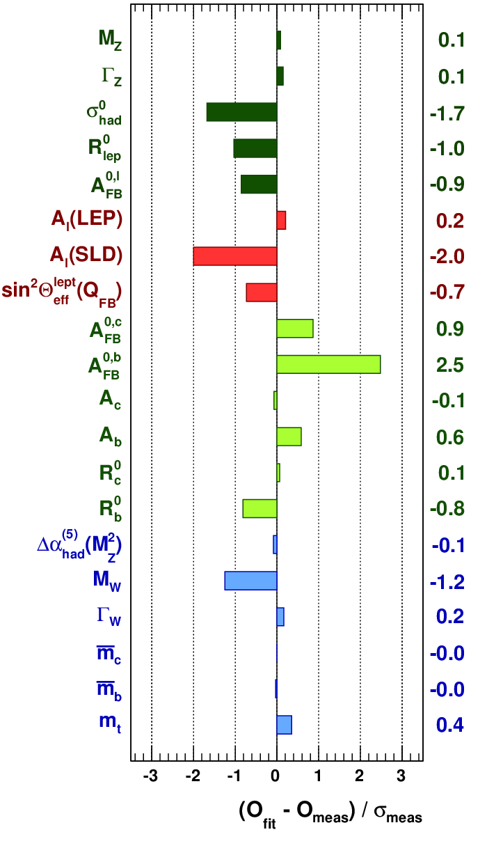
The left-hand plot of Fig. 3 gives for the complete fit the pull values obtained from the difference between the fit result and the measurement in units of the total experimental error (not including the error from the fit performed here). They reflect the known tension between the left-right asymmetry and $A_{\rm FB}^{0,b}$ , though it is noticeable that no single pull value exceeds $3\sigma$ .

Higgs mass constraints

The top and bottom plots of Fig. 4 show the profile curves of the $\Delta\chi^{2}$ test statistic for the standard and complete fits versus the $M_{H}$ parameter. In this, as in the following $\Delta\chi^{2}$ graphs, the test statistic is minimized with respect to all other freely varying fit parameters for each (fixed) value of the parameter being plotted. We find from this scan

\displaystyle M_{H}=\bigg\{\begin{array}[]{rl}91^{\>+30}_{\>-23}\>\mathrm{Ge\kern-1.00006ptV}&~~~{\rm(standard~fit)}\,,\\ 120^{\>+12}_{\>-5}\>\mathrm{Ge\kern-1.00006ptV}&~~~{\rm(complete~fit)}\,,\end{array}

with the 95% (99%) upper bounds of 163 $\mathrm{Ge\kern-1.00006ptV}$ (194 $\mathrm{Ge\kern-1.00006ptV}$ ) for the standard fit, and 143 $\mathrm{Ge\kern-1.00006ptV}$ (149 $\mathrm{Ge\kern-1.00006ptV}$ ) for the complete fit, respectively. The errors and limits include the various theory uncertainties that taken together amount to approximately $8\>\mathrm{Ge\kern-1.00006ptV}$ on $M_{H}$ .¹²¹² 12 Repeating the standard fit with all theory uncertainties fixed to zero gives $\chi^{2}_{{\rm min}}=17.2$ and $M_{H}=94^{\>+30}_{\>-24}\>\mathrm{Ge\kern-1.00006ptV}$ . A direct comparison of this result with Eq. (2.2) is not straightforward as the fit uses the additional nuisance parameters, when let free to vary, to improve the test statistics (recall the value of $\chi^{2}_{{\rm min}}=16.7$ for the standard fit result). The impact on the parameter errors would become noticeable once the input observables exhibit better compatibility (cf. discussion in Ref. [2])

The standard fit value for $M_{H}$ has moved by +8 $\mathrm{Ge\kern-1.00006ptV}$ as a consequence of the new $\Delta\alpha_{\rm had}^{(5)}(M_{Z}^{2})$ evaluation [58]. Using instead the preliminary result $\Delta\alpha_{\rm had}^{(5)}(M_{Z}^{2})=(2762.6\pm 10.3)\cdot 10^{-5}$ [66], obtained with the use of similar experimental data but less reliance on perturbative QCD, we find $M_{H}=88^{\>+29}_{\>-23}\>\mathrm{Ge\kern-1.00006ptV}$ .

The results (2.2) are obtained using the experimental world average of the direct Tevatron top mass measurements [48] whose interpretation as pole mass in theory calculations is affected with additional uncertainties (cf. discussion in Sec. 2.1). Using, for comparison, the pole mass value $m_{t}=167.5^{\>+5.0}_{\>-4.5}\>\mathrm{Ge\kern-1.00006ptV}$ [56], as determined from the $p\overline{p}\to t\overline{t}+X$ inclusive cross section, the standard electroweak fit returns for the Higgs boson mass $72^{\>+38}_{\>-25}\>\mathrm{Ge\kern-1.00006ptV}$ , which is appreciably lower than the result (2.2).

The contributions from the various measurements to the central value and uncertainty of $M_{H}$ in the standard fit are given in the right hand plot of Fig. 3, where all input measurements except for the ones listed in a given line are used in the fit. It can be seen that, e.g., precise measurements of $m_{t}$ and $M_{W}$ and a precise determination of $\Delta\alpha_{\rm had}^{(5)}(M_{Z}^{2})$ are essential for an accurate constraint of $M_{H}$ .

Figure 3 displays complementary information. Among the four observables providing the strongest constraint on $M_{H}$ , namely $A_{\ell}$ (LEP), $A_{\ell}$ (SLD), $A_{\rm FB}^{0,b}$ and $M_{W}$ , only the one indicated in a given row of the plot is included in the fit.¹³¹³ 13 The uncertainties in the free fit parameters that are correlated to $M_{H}$ (mainly $\Delta\alpha_{\rm had}^{(5)}(M_{Z}^{2})$ and $m_{t}$ ) contribute to the errors shown in Fig. 3, and generate correlations between the four $M_{H}$ values found. The compatibility among these measurements is estimated by performing a reduced standard fit in which the least compatible of the measurements (here $A_{\rm FB}^{0,b}$ ) is removed, and by comparing the $\chi^{2}_{{\rm min}}$ test statistic obtained in that fit to the one of the standard fit. The p-value of the $\chi^{2}_{{\rm min}}$ difference of 8.0 between these fits is evaluated by means of pseudo experiments, with observables fluctuating according to their experimental errors around a consistent set of SM predictions corresponding to the best-fit results for the SM parameters. In each of the pseudo experiments we follow the same procedure as for data, that is, we remove the least compatible of the measurements, refit, and compute the $\chi^{2}_{{\rm min}}$ difference with respect to the standard fit corresponding to that pseudo experiment. We find that in $(1.4\pm 0.1)\%$ (“ $2.5\sigma$ ”) of the pseudo experiments the $\chi^{2}_{{\rm min}}$ difference exceeds that observed in data.

Finally, Fig. 5 shows the p-value obtained from Monte Carlo samples of the standard fit as a function of the true Higgs mass.¹⁴¹⁴ 14 Note that by fixing $M_{H}$ the number of degrees of freedom of the fit is increased compared to the standard fit resulting in a larger average $\chi^{2}_{\rm min}$ and thus in a larger p-value. At the best-fit value of $91\>\mathrm{Ge\kern-1.00006ptV}$ the plot reproduces the goodness of the standard fit. With increasing $M_{H}$ the p-value drops reaching the $2\sigma$ level at $M_{H}=190\>\mathrm{Ge\kern-1.00006ptV}$ and the $3\sigma$ level at $M_{H}=275\>\mathrm{Ge\kern-1.00006ptV}$ .

Constraints on other parameters

The two rightmost columns of Table 1 give the results of, respectively, the complete fit and when assuming $M_{H}=120\>$ GeV (fixed) in the fit for each parameter or observable, obtained by scanning the profile likelihood without using the corresponding experimental or phenomenological constraint in the fit (indirect determination – similar to the $M_{H}$ determinations in the right-hand plot of Fig. 3). Apart from the intrinsic interest of having an indirect determination of the observables, this procedure provides interesting insight into the requirements of the fit. If the direct knowledge (first column in Table 1) of an observable is much more precise than the indirect one (last column), for example $M_{Z}$ , the variable could have been fixed in the fit without impacting the results, and thus there is no need, for the purpose of the global electroweak fit, for an improved direct determination. On the other hand, if the indirect constraint of an observable strongly outperforms the direct one, as is the case for $\Gamma_{W}$ or the direct measurement of $\sin\!^{2}\theta^{\ell}_{{\rm eff}}(Q_{\rm FB})$ , the observable is irrelevant for the fit and can be removed. To improve the indirect constraint on $M_{H}$ , the experimental efforts must focus on observables with good sensitivity to $M_{H}$ , and with competing accuracy between direct and indirect constraints, as is the case for $M_{W}$ and the $Z$ -pole asymmetries.

From these scans we obtain the following results.

•

We indirectly determine the $W$ mass from the complete fit to be

$M_{W}=80.360^{\>+0.014}_{\>-0.013}\>\mathrm{Ge\kern-1.00006ptV}\,,$ (4)

which is $1.6\sigma$ below and exceeds in precision the experimental world average [46]. Using the cross section derived $m_{t}$ value (cf. Sec. 6, page 6) we find $M_{W}=80.340^{\>+0.029}_{\>-0.021}\>\mathrm{Ge\kern-1.00006ptV}$ from the complete fit. Figure 6 shows the $\Delta\chi^{2}$ profile versus $M_{W}$ for the standard fit (green band) and the complete fit (blue band). Also shown is the world average of the direct $M_{W}$ measurements (dot with error bar). For both fits the theoretical uncertainty in the $M_{W}$ prediction ( $\delta_{\rm th}M_{W}\simeq 4\>\mathrm{Me\kern-1.00006ptV}$ ) and its treatment via the Rfit scheme leads to a broadening of the fit minima. The inclusion of the direct Higgs searches provides a considerably improved indirect $M_{W}$ determination. The grey-shaded band shows the constraint one would obtain for a hypothetical Higgs discovery at 120 $\mathrm{Ge\kern-1.00006ptV}$ with negligible error on $M_{H}$ . The precision of the indirect $M_{W}$ determination would reach $11\>\mathrm{Me\kern-1.00006ptV}$ . The uncertainty would increase to approximately $25\>\mathrm{Me\kern-1.00006ptV}$ when using the cross section derived top mass value.

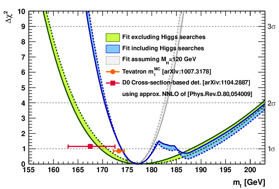
Figure 7: Indirect determination of the top quark pole mass: profile of $\Delta\chi^{2}$ versus $m_{t}$ for the complete fit (blue shaded curve) and the standard fit (green shaded curve). In both fits the direct $m_{t}$ measurement, indicated by the dot with $1\sigma$ error bar, is not included. The widths of the bands indicate the size of the cumulative theoretical uncertainty in the fit. Also shown is the pole mass result inferred by D0 from the measurement of the $p\overline{p}\to t\overline{t}+X$ cross section [56] (square dot, see text). The grey shaded curve shows the constraint one would obtain for a hypothetical Higgs discovery at 120 $\mathrm{Ge\kern-1.00006ptV}$ (with negligible error on $M_{H}$ ).
•

The indirect determination $\Delta\alpha_{\rm had}^{(5)}(M_{Z}^{2})=(2729^{\>+57}_{\>-50})\cdot 10^{-5}$ comes out slightly smaller but fully compatible with the phenomenological evaluation, while being a factor of almost five less accurate. Knowing the Higgs boson mass would only marginally improve the precision of the indirect determination (cf. last column in Table 1).
•

The strong coupling constant at the $Z$ pole to four loop perturbative order for the massless fermion propagators is found to be

$\alpha_{\scriptscriptstyle S}(M_{Z}^{2})=0.1194\pm 0.0028\,,$ (5)

with negligible theoretical uncertainty due to the good convergence of the perturbative series at that scale (cf. Ref. [2]).
•

Two local $\Delta\chi^{2}$ minima are found from the indirect constraint of the top quark pole mass in the complete fit, giving the $\Delta\chi^{2}<1$ ranges

$m_{t}=[173.8,180.6]\>\mathrm{Ge\kern-1.00006ptV}~~\rm{and}~~[185.1,189.3]\>\mathrm{Ge\kern-1.00006ptV}\,.$ (6)

The first region agrees within $1.1\sigma$ with the experimental world average of the direct $m_{t}$ measurements [48]. The separation between the two regions originates from the direct Tevatron limit on $M_{H}$ . The lower (upper) region corresponds to Higgs masses around 130 $\mathrm{Ge\kern-1.00006ptV}$ (190 $\mathrm{Ge\kern-1.00006ptV}$ ). Figure 7 shows the $\Delta\chi^{2}$ profile versus $m_{t}$ for the standard fit (green band) and the complete fit (blue band). Also shown is the world average of the direct $m_{t}$ measurements as well as the pole top mass derived from the inclusive $t\overline{t}$ cross section (dots with error bars). Similar to the indirect $M_{W}$ determination, the results from the direct Higgs searches allow to significantly increase the precision of the indirect constraint. The grey-shaded band shows the constraint on $m_{t}$ one would obtain for a hypothetical Higgs discovery at 120 $\mathrm{Ge\kern-1.00006ptV}$ with negligible error on $M_{H}$ . The precision of the indirect determination would reach $3.0\>\mathrm{Ge\kern-1.00006ptV}$ .

Figure 8: Indirect determination of the effective weak mixing angle: profile of $\Delta\chi^{2}$ versus $\sin\!^{2}\theta^{\ell}_{{\rm eff}}$ for the complete fit (blue shaded curve) and the standard fit (green shaded curve). In both fits all measurements with a direct relationship to $\sin\!^{2}\theta^{\ell}_{{\rm eff}}$ (e.g. the asymmetry parameters) are not included, and only the measured or determined values of $m_{t}$ , $M_{W}$ , $\overline{m}_{c}$ , $\overline{m}_{b}$ , $\Delta\alpha_{\rm had}^{(5)}(M_{Z}^{2})$ and $\alpha_{\scriptscriptstyle S}(M_{Z}^{2})$ are used. The widths of the bands indicate the size of the cumulative theoretical uncertainty in the fit. The LEP/SLD average for $\sin\!^{2}\theta^{\ell}_{{\rm eff}}$ as derived directly from the asymmetry measurements is indicated by the dot with $1\sigma$ error bar. The light shaded curve shows the constraint one would obtain for a hypothetical Higgs discovery at 120 $\mathrm{Ge\kern-1.00006ptV}$ (with negligible error on $M_{H}$ ).
•

For the indirect determination of the effective weak mixing angle $\sin\!^{2}\theta^{\ell}_{{\rm eff}}$ we ignore all measurements of observables that are related to $\sin\!^{2}\theta^{\ell}_{{\rm eff}}$ (e.g. the asymmetry parameters), and instead only use experimental results for $m_{t}$ , $M_{W}$ , $\overline{m}_{c}$ , $\overline{m}_{b}$ , $\Delta\alpha_{\rm had}^{(5)}(M_{Z}^{2})$ and $\alpha_{\scriptscriptstyle S}(M_{Z}^{2})$ (we use the result of Eq. (5) for the latter parameter) and the direct Higgs searches in the fit. From this we obtain the SM prediction

$\sin\!^{2}\theta^{\ell}_{{\rm eff}}=0.23148\pm 0.00011\,,$ (7)

which is compatible with and more precise than the experimental average directly derived from the asymmetry measurements at LEP and SLD: $\sin\!^{2}\theta^{\ell}_{{\rm eff}}=0.23153\pm 0.00016$ [39]. Figure 8 shows the $\Delta\chi^{2}$ profile versus $\sin\!^{2}\theta^{\ell}_{{\rm eff}}$ for the standard fit (green band) and the complete fit (blue band). Also shown is the LEP/SLD average from the direct determination. Similar to the indirect $M_{W}$ and $m_{t}$ determinations, the results from the direct Higgs searches allow to significantly increase the precision of the indirect constraint. The grey shaded band shows the constraint on $\sin\!^{2}\theta^{\ell}_{{\rm eff}}$ one would obtain for a hypothetical Higgs discovery at 120 $\mathrm{Ge\kern-1.00006ptV}$ with negligible error on $M_{H}$ .
•

Two-dimensional 68%, 95% and 99% CL allowed regions obtained from scans of fits with fixed variable pairs $M_{W}$ vs. $M_{H}$ are shown in Fig. 10. The allowed region obtained without the $M_{W}$ measurement and the direct Higgs searches (largest/blue) agrees with the world average of the direct $M_{W}$ measurements (horizontal/green band). Inclusion of the $M_{W}$ measurements (narrow/purple) reduces significantly the allowed ranges in $M_{H}$ highlighting again the importance of the $M_{W}$ measurements for an accurate $M_{H}$ determination. After the inclusion of the direct Higgs searches two separate small regions (narrowest/green) in the parameter space remain as a result of the prominent maximum around $M_{H}=160$ GeV in Fig. 4 (bottom).
•

Two-dimensional 68%, 95% and 99% CL allowed regions obtained from scans of fits with fixed variable pairs $M_{W}$ vs. $m_{t}$ are shown in Fig. 10. The indirect determination (largest/blue) without the $M_{W}$ and $m_{t}$ measurements and without the direct Higgs searches shows agreement with the direct $M_{W}$ and $m_{t}$ measurements (horizontal and vertical green bands). The inclusion of the results of the direct Higgs searches reduces significantly the allowed region (narrow/yellow), which is still in agreement with the direct results. For illustration, isolines for various values of $M_{H}$ representing the SM prediction in an indicative way are also shown. As these isolines do not include the theoretical uncertainties (e.g. on $M_{W}$ ), the allowed region of the fit including the direct Higgs searches (narrow/yellow region) as shown in this plot extend slightly into regions of $M_{H}$ values smaller than the strict exclusion bound from LEP ( $M_{H}<114.4$ GeV). For the same reason the 2-dimensional region allowed from the fit is not split into two separate region as naively expected from the Higgs boson mass limits around $M_{H}=160$ GeV.

More results and plots for the global SM fit are available on the Gfitter web site [67].

3 Oblique Corrections

A common approach to constrain physics beyond the SM using the global electroweak fit is through the formalism of oblique parameters.

3.1 Concept of oblique parameters

Provided that the new physics mass scale is high, beyond the scale of direct production, and that it contributes only through virtual loops to the electroweak precision observables, the dominant BSM effects can be parametrised by three gauge boson self-energy parameters named oblique parameters. In this section we recall only the relevant parameter definitions. A more general introduction of the oblique formalism is given in the appendix, page A.

The literature focuses on two different, but equivalent oblique parameter sets: $\varepsilon_{1,2,3}$ [68, 69] and $S,\,T,\,U$ [6]. Both sets are reparametrisations of the variables $\Delta\rho$ , $\Delta\kappa$ and $\Delta r$ , which absorb the radiative corrections to the total $Z$ coupling strength, the effective weak mixing angle, and the $W$ mass, respectively. It is assumed that the new physics contributing to the radiative corrections is flavour universal, while for the $Z\to b\overline{b}$ vertex, receiving large top-quark corrections, an extra oblique parameter is introduced. In this analysis we implement the additional corrections to the $Z\to b\overline{b}$ coupling as described in Ref. [70]. More parameters $(X,Y,V,W)$ are required if the scale of new physics is not much larger than the weak scale [71, 72]. They can only be independently determined when including data at higher centre-of-mass energies than the $Z$ pole, which is not carried out in the present analysis, so that these additional parameters are set to zero.

The $\varepsilon_{1,2,3}$ parameters [68, 69] include SM contributions dominated by top quark and Higgs boson corrections. By construction they vanish at Born level if the running of $\alpha$ is accounted for. Their typical size is hence of order $\alpha$ . They are defined by

$\displaystyle\varepsilon_{1}$	$\displaystyle\!\!=\!\!$	$\displaystyle\Delta\rho\,,$	(8)
$\displaystyle\varepsilon_{2}$	$\displaystyle\!\!=\!\!$	$\displaystyle\cos^{2}\!\theta_{W}\Delta\rho+\frac{\sin^{2}\!\theta_{G}}{\cos^{2}\!\theta_{W}-\sin^{2}\!\theta_{G}}\Delta r-2\sin^{2}\!\theta_{G}\Delta\kappa^{\prime}\,,$	(9)
$\displaystyle\varepsilon_{3}$	$\displaystyle\!\!=\!\!$	$\displaystyle\cos^{2}\!\theta_{W}\Delta\rho+(\cos^{2}\!\theta_{W}-\sin^{2}\!\theta_{G})\Delta\kappa^{\prime}\,,$	(10)

with $2\sin^{2}\!\theta_{G}=1-\sqrt{1-\sqrt{8}\pi\alpha(M_{Z}^{2})/(G_{F}M_{Z}^{2})}$ and where $\Delta\kappa^{\prime}$ relates $\sin\!^{2}\theta^{f}_{{\rm eff}}$ to $\sin^{2}\!\theta_{G}$ instead of $\sin^{2}\!\theta_{W}$ . The quadratic top mass dependence present in all form factors has been removed explicitly from the parameters $\varepsilon_{2}$ and $\varepsilon_{3}$ .

In the definition of the $S,\,T,\,U$ parameters [6] the predicted SM contributions are subtracted from the measured $\varepsilon$ parameters, so that the $S,\,T,\,U$ vanish in the SM. Due to the dominant virtual top quark and Higgs boson corrections, the subtracted SM terms depend on $M_{H}$ and $m_{t}$ , which take fixed reference values. Thus, by construction, the $S,\,T,\,U$ parameters depend on a (somewhat arbitrary) SM reference point, while the physically relevant difference between the experimental $S,\,T,\,U$ parameters and a model prediction is independent of the reference. The $S,\,T,\,U$ parameter are normalised so that the expected BSM contributions are of order ${\cal O}(1)$ . The so subtracted and normalised parameters are related to the $\varepsilon$ parameters by

$\displaystyle S$	$\displaystyle\!\!=\!\!$	$\displaystyle+\varepsilon_{3}\frac{4\sin^{2}\!\theta_{G}}{\alpha(M_{Z}^{2})}-d_{S}\,,$	(11)
$\displaystyle T$	$\displaystyle\!\!=\!\!$	$\displaystyle\phantom{\pm}\varepsilon_{1}\frac{1}{\alpha(M_{Z}^{2})}-d_{T}\,,$	(12)
$\displaystyle U$	$\displaystyle\!\!=\!\!$	$\displaystyle-\varepsilon_{2}\frac{4\sin^{2}\!\theta_{G}}{\alpha(M_{Z}^{2})}-d_{U}\,,$	(13)

where $d_{i}$ are the SM predictions for the chosen $M_{H}$ and $m_{t}$ reference. Throughout this paper we use the reference values $M_{H,\rm ref}=120$ GeV and $m_{t,\rm ref}=173$ GeV that are chosen to agree with the experimental constraints.

Physics beyond the SM can also contribute to the $Z\to b\overline{b}$ vertex, which receives significant top quark corrections in the SM. Following Ref. [70] these additional vertex corrections are implemented via two new parameters, $\delta g_{L}^{b\overline{b}}$ and $\delta g_{R}^{b\overline{b}}$ . These parameters are set to zero in the fits determining the experimental values of the $S,\,T,\,U$ parameters. The parameters are included for new physics models that significantly contribute to the $Z\to b\overline{b}$ vertex, which, for the models studied in this paper, is only the case for the Littlest Higgs model (cf. Section 4.4).

The advantage of the $S,\,T,\,U$ parametrisation lies in the convenience with which it permits to compare model predictions with the electroweak data. It is therefore adopted in most parts of this paper. For a given model, the prediction of any electroweak observable $O$ is given by

O=O_{\rm SM,ref}(M_{H,\rm ref},m_{t,\rm ref})+c_{S}S+c_{T}T+c_{U}U\,,

(14)

where $O_{\rm SM,ref}(M_{H,\rm ref},m_{t,\rm ref})$ is the SM prediction of the observable in the reference SM, including all known two-loop and beyond two-loop electroweak corrections. The linear terms ( $c_{S}S$ , $c_{T}T$ , $c_{U}U$ ) parametrise the additional contribution from the BSM model. The coefficients $c_{S},c_{T},c_{U}$ are available in the literature for the full set of electroweak precision observables. This report uses the values from Ref. [73]. The precise measurements of the electroweak observables thus allow to constrain $S,\,T,\,U$ , and hence parameters of specific BSM physics models whose contributions to the oblique parameters have been calculated.

The BSM effects on the $S,\,T,\,U$ parameters can be summarised as follows.

•

The $T$ parameter measures the difference between the new physics contributions of neutral and charged current processes at low energies, i.e. it is sensitive to weak isospin violation. $T$ ( $\varepsilon_{1}$ ) is proportional to $\Delta\rho$ .
•

The $S$ $(S+U)$ parameter describes new physics contributions to neutral (charged) current processes at different energy scales. The $S$ parameter ( $\varepsilon_{3}$ ) takes the remaining part of $\Delta\kappa$ , which is then free from quadratic top quark contributions due to weak-isospin breaking.
•

The third parameter, $U$ , is only constrained by the $W$ boson mass and width. $U$ ( $\varepsilon_{2}$ ) describes the remaining corrections to $\Delta r$ and is predicted to be small in most new physics models.

Updated experimental results for the oblique parameters as obtained from the global electroweak fit are given in the following section. Similar studies have been performed by the LEP Electroweak Working Group [3] and for the electroweak review of the Particle Data Group [4].

3.2 Experimental constraints on the oblique parameters

The $S,\,T,\,U$ parameters are determined from the fit by comparing the measured electroweak precision observables with the respective theory predictions of Eq. (14). Except for the fixed $M_{H,\rm ref}$ and $m_{t,\rm ref}$ all other SM fit parameters, including $S$ , $T$ and $U$ , are free to vary in the fit (cf. bold quantities in Table 1). After fit convergence we find

S=0.03\pm 0.10\,,\quad\quad\quad T=0.05\pm 0.12\,,\quad\quad\quad U=0.07\pm 0.11\,,

(15)

and linear correlation coefficients of $+0.89$ between $S$ and $T$ , and $-0.49$ ( $-0.72$ ) between $S$ and $U$ ( $T$ and $U$ ). Some BSM models predict a vanishing or negligible contribution to $U$ , which allows to stronger constrain the remaining parameters. Fixing $U=0$ we obtain

S|_{U=0}=0.06\pm 0.09,\quad\quad\quad T|_{U=0}=0.10\pm 0.08,

(16)

with a correlation coefficient of $+0.89$ . The improved precision on $S$ and $T$ stems from the information of $M_{W}$ and $\Gamma_{W}$ , which otherwise is absorbed to determine the $U$ parameter.

As all the experimental $S,\,T,\,U$ values are compatible with zero, the data are in agreement with our chosen SM reference. Figures 11 and 12 show by the orange ellipses the 68%, 95% and 99% confidence level (CL) allowed regions in the $(S,T)$ , $(S,U)$ and $(U,T)$ planes. Figure 11 also gives the tighter constraints found when fixing $U=0$ (blue ellipses). The upper panel displays for $U=0$ the individual constraints from the asymmetry measurements, $Z$ partial and total widths, and $W$ mass and width. Leaving $U$ free would leave the former two constraints approximately unchanged, while the $W$ mass and width would then constrain $U$ rather than $S$ or $T$ . Also shown on all plots is the SM prediction for varying $M_{H}$ and $m_{t}$ values (ranges given on plots). By construction, the SM prediction reproduces $S=T=U=0$ at the $\rm SM_{ref}$ bench mark. While the variations of $S,T,U$ within the current $m_{t}$ uncertainty is small, $M_{H}$ values larger than the electroweak scale lead to larger (smaller) values of $S$ $(T)$ . The $U$ parameter exhibits only a small dependence on $M_{H}$ , justifying the choice $U=0$ for the SM interpretation. All experimentally allowed ellipses show compatibility with the SM predictions for a light Higgs boson, reflecting the satisfactory goodness-of-fit obtained in the SM fit (cf. Section 2.2).¹⁵¹⁵ 15 Had we determined $M_{H}$ by confronting experimental and predicted oblique parameters, we would reproduce Fig. 4 up to deviations due to the higher order and non-oblique corrections present in the standard electroweak fit.

Many BSM models feature a similar agreement with the data as observed for the SM. The predictions of these models can cover large regions in the $(S,T,U)$ space due to additional undetermined model parameters, which in turn can be constrained via the oblique parameter formalism from the data. Most (though not all) models decouple at high scales from the SM so that the oblique corrections reproduce the SM values. We will see in the following that models providing additional weak isospin violation can readily accommodate large Higgs boson masses, whose negative $T$ values are compensated by the model-induced positive contributions.

4 Constraints on New Physics Models

We proceed the analysis with confronting the $S,\,T,\,U$ parameters determined in the previous section with predictions from SM extensions. For a given new physics model, the $S,\,T,\,U$ predictions consist of the sum of the BSM contributions and the non-vanishing SM remainders when the $M_{H}$ and $m_{t}$ values differ from those used for the SM reference. Numerous oblique parameter analyses have been performed in the past, usually following two separate steps: $(i)$ the determination of the $S,\,T,\,U$ parameters by groups performing the electroweak fit, and $(ii)$ BSM studies using these $S,\,T,\,U$ values in independent analyses. When fitting the BSM model parameters together with the top quark and Higgs boson masses, the dependence of $S,\,T,\,U$ on the latter two parameters is then usually approximated by the one-loop terms [6]

$\displaystyle S$	$\displaystyle\!\!\approx\!\!$	$\displaystyle\frac{1}{12\pi}\ln\!\frac{M_{H}^{2}}{M_{H,\rm ref}^{2}}+\frac{1}{6\pi}\ln\frac{m_{t}^{2}}{m_{t,\rm ref}^{2}}\,,$	(17)
$\displaystyle T$	$\displaystyle\!\!\approx\!\!$	$\displaystyle-\frac{3}{16\pi\cos^{2}\!\theta_{W}}\ln\!\frac{M_{H}^{2}}{M_{H,\rm ref}^{2}}+\frac{3}{16\pi\sin^{2}\!\theta_{W}\cos^{2}\!\theta_{W}}\ln\frac{m_{t}^{2}-m_{t,\rm ref}^{2}}{m_{Z}^{2}}\,,$	(18)
$\displaystyle U$	$\displaystyle\!\!\approx\!\!$	$\displaystyle\frac{1}{2\pi}\ln\frac{m_{t}^{2}}{m_{t,\rm ref}^{2}}\,.$	(19)

The $m_{t}$ dependence is often neglected. The Gfitter software allows us to study the dependence of the oblique corrections on the BSM model parameters and the SM parameters ( $M_{H}$ and $m_{t}$ ) taking into account the full two-loop and beyond-two-loop corrections of the SM.

In this section we revisit published $S,\,T,\,U$ predictions for several prominent BSM models and provide BSM constraints derived with consistent electroweak data (as used in Sect. 2 for the standard fit), SM reference point and statistical procedure. At the beginning of each subsection we provide a brief outline of the main model features and recall the available experimental search results. None of the direct searches is used to constrain the $S,\,T,\,U$ predictions or new physics parameter fits.

4.1 Models with a sequential fourth fermion generation

The fermion sector of the SM is composed of three generations of leptons and quarks. Several SM extensions suggest extra families of matter particles, which – with the dawn of the LHC – have received increased attention in the theoretical literature. As the new fermions would obtain their masses via Yukawa couplings to the Higgs condensate they must be of order the electroweak scale and hence should be experimentally accessible. The phenomenological consequences of a fourth generation on the flavour sector of neutrinos, charged leptons and quarks have been extensively explored (cf., e.g., Refs. [74, 75, 76, 77, 78, 79, 80, 81, 82, 83, 84, 85] and the review [86]). The impact on electroweak precision data at the $Z$ -pole and on Higgs physics has been studied in Refs. [87, 88, 89, 90, 91, 92, 93, 80]. For the present analysis, we use the oblique corrections computed in Ref. [89].

In a generic model with only one extra generation, two new fermions $(\psi_{1},\psi_{2})$ , with one left-handed weak isospin doublet $\psi_{L}=(\psi_{1},\psi_{2})_{L}$ and two right-handed weak isospin singlet states $\psi_{1,R}$ , $\psi_{2,R}$ , and with charges equal to the three SM generations, are added to each of the quark and lepton sectors. The new unconstrained model parameters are the masses $m_{u_{4}}$ , $m_{d_{4}}$ , $m_{\nu_{4}}$ , $m_{e_{4}}$ of the fourth generation quarks and leptons, and $C\!P$ -conserving and $C\!P$ -violating neutrino and quark mixing parameters. The fourth generation neutrino must have a mass of at least $M_{Z}/2$ to not contribute to the invisible width of the $Z$ .

The most stringent experimental lower limits on sequential heavy fourth generation quarks (SM4) stem from CMS [94], excluding $d_{4}$ masses between 255 and 361 GeV, and from the Tevatron experiments where the newest analyses from CDF exclude $u_{4}$ quarks below 358 GeV and $d_{4}$ quarks below 372 GeV [95, 96]. The $u_{4}$ searches assume predominant decays into $W$ boson and SM quarks, requiring a small $u_{4}$ – $d_{4}$ mass splitting to inhibit the decay $u_{4}\to Wd_{4}$ . The CMS and Tevatron $d_{4}$ searches assume a $d_{4}\to Wt$ branching fraction of one on the basis of the observed unitarity of the three-generation CKM quark mixing matrix suggesting small flavour-changing currents to light quarks. This also neglects the possibility of an inverted fourth generation mass hierarchy. The CDF limits have been reanalysed in Refs. [97, 98] under more general SM4 and CKM4 quark mixing scenarios, leading to a weaker limit of 290 GeV for both quark flavours. Fourth generation leptons have been best constrained at LEP with a lower limit of about 101 GeV for sequential heavy leptons decaying to $W\nu$ and $Z\ell$ , or to $W\ell$ and $Z\nu$ , depending on their electromagnetic charge [99].

Assuming negligible mixing of the extra fermions with the SM fermions,¹⁶¹⁶ 16 A detailed numerical SM4 analysis [80] taking into account low-energy FCNC processes in the quark sector, electroweak oblique corrections, and lepton decays (but not lepton mixing) concludes that small mixing between the quarks of the first three and those of the fourth family is favoured. The value of $|V_{tb}|$ is found in this analysis to exceed 0.93. The no-mixing assumption allows us to use the measured value of $G_{F}$ , extracted from the muon lifetime under the SM3 hypothesis, to its full precision [84]. the one-loop fermionic contributions of a sequential fourth generation to the oblique corrections are given by [89]

$\displaystyle S$	$\displaystyle=$	$\displaystyle\frac{{N_{\scriptscriptstyle C}}}{6\pi}\bigg\{(8Y+6)x_{1}-(8Y-6)x_{2}-2Y\ln\frac{x_{1}}{x_{2}}$	(20)
		$\displaystyle\hskip 25.6073pt+\;\left[\left(\frac{3}{2}+2Y\right)x_{1}+Y\right]G(x_{1})+\left[\left(\frac{3}{2}-2Y\right)x_{2}-Y\right]G(x_{2})\bigg\}\,,$	(20)
$\displaystyle T$	$\displaystyle=$	$\displaystyle\frac{{N_{\scriptscriptstyle C}}}{8\pi s^{2}_{W}c^{2}_{W}}F(x_{1},x_{2})\,,$	(21)
$\displaystyle U$	$\displaystyle=$	$\displaystyle-\frac{{N_{\scriptscriptstyle C}}}{2\pi}\bigg\{\frac{1}{2}(x_{1}+x_{2})-\frac{1}{3}(x_{1}-x_{2})^{2}+\left[\frac{1}{6}(x_{1}-x_{2})^{3}-\frac{1}{2}\frac{x_{1}^{2}+x_{2}^{2}}{x_{1}-x_{2}}\right]\ln\frac{x_{1}}{x_{2}}$	(22)
		$\displaystyle\hskip 39.83368pt+\;\frac{1}{6}(x_{1}-1)f(x_{1},x_{1})+\frac{1}{6}(x_{2}-1)f(x_{2},x_{2})$
		$\displaystyle\hskip 39.83368pt+\;\left[\frac{1}{3}-\frac{1}{6}(x_{1}+x_{2})-\frac{1}{6}(x_{1}-x_{2})^{2}\right]f(x_{1},x_{2})\bigg\}\,,$

where $Y=1/6\,(-1/2)$ is the weak hypercharge for quarks (leptons), ${N_{\scriptscriptstyle C}}=3\,(1)$ for quarks (leptons), $x_{i}=(m_{i_{4}}/M_{Z})^{2}$ with $i=1,2$ for the up-type and down-type fourth generation fermions, respectively.¹⁷¹⁷ 17 The functions in Eqs. (20–22) are defined as follows. $F(x_{1},x_{2})=(x_{1}+x_{2})/2-x_{1}x_{2}/(x_{1}-x_{2})\cdot\ln(x_{1}/x_{2})$ , $G(x)=-4y\arctan(1/y)$ , $y=\sqrt{4x-1}$ , and $f(x_{1},x_{2})=-2\sqrt{\Delta}[\arctan((x_{1}-x_{2}+1)/\sqrt{\Delta})-\arctan((x_{1}-x_{2}-1)/\sqrt{\Delta})]$ for $\Delta>0$ , $f(x_{1},x_{2})=0$ for $\Delta=0$ , and $f(x_{1},x_{2})=\sqrt{-\Delta}\cdot\ln((X+\sqrt{-\Delta})/(X-\sqrt{-\Delta}))$ with $X=x_{1}+x_{2}-1$ for $\Delta<0$ , and where $\Delta=2(x_{1}+x_{2})-(x_{1}-x_{2})^{2}-1$ .

In the limit of large and degenerate up and down-type fermion masses, the $S$ parameter in Eq. (20) reduces to $2/(3\pi)\simeq 0.21$ , exhibiting the non-decoupling property of fourth generation models. Small fourth generation quark and lepton masses lead to larger positive $S$ values that, with increasing up $\,>\,$ down mass splitting decrease (increase) for quarks (leptons). Negative contributions to $S$ are possible for a heavier up-type than down-type quark, or for a heavier charged lepton than neutrino (e.g., for $m_{\nu_{4}}=400$ $\mathrm{Ge\kern-1.00006ptV}$ and $m_{e_{4}}=660$ $\mathrm{Ge\kern-1.00006ptV}$ one has $\Delta S_{\ell}\simeq-0$ ).

The $T$ parameter (21), sensitive to weak isospin violation, is always positive or zero, owing to $F(x_{1},x_{2})\geq 0$ , $\forall x_{1},x_{2}>0$ . In case of approximate mass degeneracy, $T$ is proportional to the difference between up and down-type mass-squared relative to $M_{Z}^{2}$ .

The $U$ parameter (22) is positively defined and vanishes for degenerate fourth generation up-type and down-type fermion masses. For freely varying masses within the range $[100,1000]$ GeV, the maximum value, obtained at maximum mass splitting, reads: $U\simeq 0.49_{q}+0.16_{\ell}\simeq 0.66$ .

Figure 13 shows the experimental fit result in the $(S,T)$ plane for free $U$ together with the prediction from a fourth fermion generation with vanishing mixing. The markers indicate special model settings corresponding to the fixed masses $m_{\nu_{4}}=120\>\mathrm{Ge\kern-1.00006ptV}$ , $m_{e_{4}}=200\>\mathrm{Ge\kern-1.00006ptV}$ , $m_{d_{4}}=400\>\mathrm{Ge\kern-1.00006ptV}$ , and various choices for $m_{u_{4}}$ and $M_{H}$ .¹⁸¹⁸ 18 Ignoring flavour mixing between the fourth and the SM generations, it was found in Ref. [100] that absolute vacuum stability of the running Higgs self coupling approximately requires the mass hierarchy $M_{H}\gtrsim m_{u_{4}}$ . This strong lower bound on the Higgs boson mass may possibly be weakened by looser stability requirements. For example, in SM3 the absolute stability lower bound on $M_{H}$ is significantly reduced by allowing the minimum potential to be metastable with finite probability not to have tunnelled into another, deeper minimum during the lifetime of the universe [101, 102]. In the following discussion we will ignore the stability bound on $M_{H}$ . The $T$ parameter grows with the amount of the up and down-type fermion mass splitting, while the $S$ parameter logarithmically grows with $M_{H}$ from the SM contribution, prevailing over the opposite trend from the increasing $m_{u_{4}}$ . The shaded area in Fig. 13 depicts the allowed region when letting the fourth generation quark (lepton) masses free to vary within the interval $[200,1000]\,\mathrm{Ge\kern-1.00006ptV}$ ( $[100,1000]\,\mathrm{Ge\kern-1.00006ptV}$ ), and $M_{H}$ within $[100,1000]\,\mathrm{Ge\kern-1.00006ptV}$ . For specific parameter settings the fourth generation model is in agreement with the experimental data, and large values of $M_{H}$ are allowed.

Because the oblique parameters are mainly sensitive to the mass differences between the up-type and down-type fermions instead of their absolute mass values, we have derived in Fig. 14 the 68%, 95% and 99% CL allowed regions in the $(m_{u_{4}}-m_{d_{4}},m_{l_{4}}-m_{{\nu}_{4}})$ plane. Shown are the constraints obtained for, from the top left to the bottom right panel, increasing values of $M_{H}$ . Large $M_{H}$ values of up to $1\>\mathrm{Te\kern-1.00006ptV}$ can be accommodated by the data if the negative $T$ shift induced by $M_{H}$ is cancelled by a corresponding positive shift from a large fermion mass splitting. The data prefer a heavier charged lepton to counterweight the $S$ increase from the increasing $M_{H}$ .

A sequential fourth generation of heavy quarks would increase the gluon fusion to Higgs production cross section, dominantly mediated by a triangular top loop, by approximately a factor of nine, hence increasing the experimental Higgs boson discovery and exclusion potential. The Tevatron experiments [103], ATLAS [63] and CMS [64] have reinterpreted their negative Higgs boson search results in the channel $H\to WW$ in terms of four generations obtaining the 95% CL exclusion bounds $131<M_{H}<204\>$ GeV, $140<M_{H}<185\>$ GeV and $144<M_{H}<207\>$ GeV, respectively. Inserting these bounds into Fig. 13 does not alter the allowed $(S,T)$ region of the fourth generation model. It also does not affect the allowed fermion mass parameters shown in Fig. 13, which were chosen to escape the excluded $M_{H}$ region.

4.2 Two-Higgs Doublet Model

Two-Higgs doublet models (2HDM) [104] are simple extensions to the SM Higgs sector, which introduce one additional $SU(2)_{L}\times U(1)_{Y}$ Higgs doublet with hypercharge $Y=1$ . Two Higgs doublets lead to five physical Higgs boson states of which three, $h^{0}$ , $H^{0}$ , $A^{0}$ , are electrically neutral and the two remaining ones, $H^{\pm}$ , are electrically charged. Of the neutral states, $h^{0}$ and $H^{0}$ are scalars and $A^{0}$ is pseudoscalar. The free parameters of the 2HDM are the Higgs boson masses $M_{h^{0}}$ , $M_{H^{0}}$ , $M_{A^{0}}$ and $M_{H^{\pm}}$ , the ratio of the vacuum expectation values of the two Higgs doublets, $\tan\!\beta=v_{2}/v_{1}$ , occurring in the mixing of charged and neutral Higgs fields, and the angle $\alpha$ governing the mixing of the neutral $C\!P$ -even Higgs fields. In the most general 2HDM $\tan\!\beta$ and, hence, the corresponding Higgs couplings and mass matrix elements depend on the choice of basis for the Higgs fields [105, 106].

Models with two Higgs doublets intrinsically fulfil the empirical equality $M_{W}^{2}\approx M_{Z}^{2}\cos^{2}\theta_{W}$ . They also increase the maximum allowed mass of the lightest neutral Higgs boson for electroweak baryogenesis scenarios to values not yet excluded by LEP (see e.g., Ref. [107]) and they allow for $C\!P$ violation in the Higgs sector. Flavour changing neutral currents can be suppressed with an appropriate choice of the Higgs-to-fermion couplings (see e.g., Ref. [95, 108]). For example, in the Type-I 2HDM this is achieved by letting only one Higgs doublet couple to the fermion sector. In the Type-II 2HDM [109] one Higgs doublet couples to the up-type quarks and leptons only, while the other one couples to the down-type fermions. The Type-II 2HDM resembles the Higgs sector of the Minimal Supersymmetric Standard Model. It fixes the basis of the Higgs fields and promotes $\tan\!\beta$ to a physical parameter.

Our previous analysis of the Type-II 2HDM extension [2] was restricted to the $C\!P$ conserving 2HDM scalar potential, and only included observables sensitive to corrections from the exchange of a charged Higgs boson. The most constraining of these observables involve rare radiative or leptonic decays of $B$ and $K$ mesons, where the charged current mediated by the $W$ is replaced by a charged Higgs. The combination of the constraints obtained excludes the high- $\tan\!\beta$ , low- $M_{H^{\pm}}$ region spared by the $B\to\tau\nu$ constraint, and leads to a 95% CL charged-Higgs exclusion below $240\>\mathrm{Ge\kern-1.00006ptV}$ , irrespective of the value of $\tan\!\beta$ . This limit increases towards larger $\tan\!\beta$ , e.g., $M_{H^{\pm}}<780\>\mathrm{Ge\kern-1.00006ptV}$ are excluded for $\tan\!\beta=70$ at 95% CL. A similar analysis, which also includes neutral $B^{0}$ meson mixing, has been reported in Ref. [110]. There, a $\tan\!\beta$ independent 95% CL lower limit of $316\>\mathrm{Ge\kern-1.00006ptV}$ was achieved.

Direct searches for the charged Higgs within the Type-II 2HDM have been performed by the LEP collaborations. The main limitations were background from diboson production and the kinematic limitation on the production cross section [111, 112, 113, 114]. The combined limit determined by the LEP Higgs Working Group is $M_{H^{\pm}}>\rm 78.6\>GeV$ [115].

For the study of the 2HDM oblique corrections the type distinction between the models is irrelevant as they are defined according to the Yukawa couplings, which do not enter the oblique corrections at one-loop order. For the prediction of the $S,\,T,\,U$ parameters we use the formulas of Refs. [116, 117, 118]¹⁹¹⁹ 19 The functions defined in Eqs. (23–25) are defined as follows. $\mathcal{B}_{22}(q^{2},m_{1}^{2},m_{2}^{2})=q^{2}/24\{2\ln q^{2}+\ln(x_{1}x_{2})+[(x_{1}-x_{2})^{3}-3(x_{1}^{2}-x_{2}^{2})+3(x_{1}-x_{2})]\ln(x_{1}/x_{2})-\left[2(x_{1}-x_{2})^{2}-8(x_{1}+x_{2})+10/3\right]-[(x_{1}-x_{2})^{2}-2(x_{1}+x_{2})+1]f(x_{1},x_{2})-6F(x_{1},x_{2})\}\overset{m_{1}=m_{2}}{\Rightarrow}q^{2}/24\left[2\ln q^{2}+2\ln x_{1}+\left(16x_{1}-10/3\right)+(4x_{1}-1)G(x_{1})\right]$ , where $x_{i}\equiv m_{i}^{2}/q^{2}$ , $\mathcal{B}_{0}(q^{2},m_{1}^{2},m_{2}^{2})=1+1/2\left[(x_{1}+x_{2})/(x_{1}-x_{2})-(x_{1}-x_{2})\right]\ln(x_{1}/x_{2})+1/2f(x_{1},x_{2})\overset{m_{1}=m_{2}}{\Rightarrow}2-2y\arctan(1/y),\quad y=\sqrt{4x_{1}-1}$ , $\overline{B}_{0}(m_{1}^{2},m_{2}^{2},m_{3}^{2})=(m_{1}^{2}\ln m_{1}^{2}-m_{3}^{2}\ln m_{3}^{2})/(m_{1}^{2}-m_{3}^{2})-(m_{1}^{2}\ln m_{1}^{2}-m_{2}^{2}\ln m_{2}^{2})/(m_{1}^{2}-m_{2}^{2})$ [89], see also Footnote 17 on page 17. .

$\displaystyle S$	$\displaystyle=$	$\displaystyle\frac{1}{\pi M_{Z}^{2}}\bigg\{\sin^{2}(\beta-\alpha)\mathcal{B}_{22}(M_{Z}^{2},M_{H^{0}}^{2},M_{A^{0}}^{2})-\mathcal{B}_{22}(M_{Z}^{2},M_{H^{\pm}}^{2},M_{H^{\pm}}^{2})$	(23)
		$\displaystyle+\;\cos^{2}(\beta-\alpha)\bigg[\mathcal{B}_{22}(M_{Z}^{2},M_{h^{0}}^{2},M_{A^{0}}^{2})+\mathcal{B}_{22}(M_{Z}^{2},M_{Z}^{2},M_{H^{0}}^{2})-\mathcal{B}_{22}(M_{Z}^{2},M_{Z}^{2},M_{h^{0}}^{2})$
		$\displaystyle-\;M_{Z}^{2}\mathcal{B}_{0}(M_{Z}^{2},M_{Z}^{2},M_{H^{0}}^{2})+M_{Z}^{2}\mathcal{B}_{0}(M_{Z}^{2},M_{Z}^{2},M_{h^{0}}^{2})\bigg]\bigg\}\,,$
$\displaystyle T$	$\displaystyle=$	$\displaystyle\frac{1}{16\pi M_{W}^{2}\sin^{2}\theta_{W}}\bigg\{F(M_{H^{\pm}}^{2},M_{A^{0}}^{2})+\sin^{2}(\beta-\alpha)\bigg[F(M_{H^{\pm}}^{2},M_{H^{0}}^{2})-F(M_{A^{0}}^{2},M_{H^{0}}^{2})\bigg]$	(24)
		$\displaystyle+\;\cos^{2}(\beta-\alpha)\bigg[F(M_{H^{\pm}}^{2},M_{h^{0}}^{2})-F(M_{A^{0}}^{2},M_{h^{0}}^{2})+F(M_{W}^{2},M_{H^{0}}^{2})-F(M_{W}^{2},M_{h^{0}}^{2})$
		$\displaystyle-F(M_{Z}^{2},M_{H^{0}}^{2})+F(M_{Z}^{2},M_{h^{0}}^{2})+4M_{Z}^{2}\overline{B}_{0}(M_{Z}^{2},M_{H^{0}}^{2},M_{h^{0}}^{2})-4M_{W}^{2}\overline{B}_{0}(M_{W}^{2},M_{H^{0}}^{2},M_{h^{0}}^{2})\bigg]\bigg\}\,,$

$\displaystyle U$	$\displaystyle=$	$\displaystyle-S+\frac{1}{\pi M_{Z}^{2}}\bigg\{\mathcal{B}_{22}(M_{W}^{2},M_{A^{0}}^{2},M_{H^{\pm}}^{2})-2\mathcal{B}_{22}(M_{W}^{2},M_{H^{\pm}}^{2},M_{H^{\pm}}^{2})$	(25)
		$\displaystyle+\;\sin^{2}(\beta-\alpha)\mathcal{B}_{22}(M_{W}^{2},M_{H^{0}}^{2},M_{H^{\pm}}^{2})$
		$\displaystyle+\;\cos^{2}(\beta-\alpha)\bigg[\mathcal{B}_{22}(M_{W}^{2},M_{h^{0}}^{2},M_{H^{\pm}}^{2})+\mathcal{B}_{22}(M_{W}^{2},M_{W}^{2},M_{H^{0}}^{2})-\mathcal{B}_{22}(M_{W}^{2},M_{W}^{2},M_{h^{0}}^{2})$
		$\displaystyle-\;M_{W}^{2}\mathcal{B}_{0}(M_{W}^{2},M_{W}^{2},M_{H^{0}}^{2})+M_{W}^{2}\mathcal{B}_{0}(M_{W}^{2},M_{W}^{2},M_{h^{0}}^{2})\bigg]\bigg\}\,.$

Figure 15 shows the 68%, 95%, and 99% CL allowed contours in the ( $S,T$ )-plane (letting $U$ vary freely) as derived in the electroweak fit together with the SM and 2HDM predictions (grey and green areas, respectively). For the 2HDM prediction $M_{h^{0}}$ was left free to vary within [114,1000] GeV and the masses of the other Higgs bosons were allowed to vary between $M_{h^{0}}$ and $1000\>$ GeV. $S$ adopts relatively small and mainly positive values, whereas the contribution to $T$ can take large positive and negative values. There is a large overlap between the experimental fit and the 2HDM prediction, so that a variety of model configurations exhibits compatibility with the electroweak precision data. A few of these configurations are shown for fixed values of $M_{h^{0}}=\rm 600\>GeV$ , $M_{A^{0}}=\rm 900\>GeV$ , and $\beta-\alpha=\frac{\pi}{2}$ in Fig. 15. The open symbols depict the predictions for three different masses of the lightest Higgs ( $M_{h^{0}}=\rm 120,\,250,\,500\>GeV$ ) and a fixed charged Higgs mass of $580\>$ GeV. The arrows indicate the 2HDM-induced shifts in $S$ and $T$ with respect to the SM prediction for the same $M_{h^{0}}$ values. Variations of the charged Higgs mass (full symbols) induce strong effects on $T$ . By choosing adequate values ( $M_{H^{\pm}}=\rm 590,\,570,\,550\>GeV$ ) compatibility with the electroweak data can be achieved even for large $M_{h^{0}}$ .

Further 2HDM parameter configurations that are allowed by the electroweak data are shown in Fig. 16. For fixed $M_{H^{0}}$ , $M_{A^{0}}$ , and $\beta-\alpha$ , only two small bands of $M_{H^{\pm}}$ are allowed, namely masses very similar to either $M_{H^{0}}$ or $M_{A^{0}}$ , whereas $M_{h^{0}}$ cannot be constrained (see Fig 16 (top left)) other than being the lightest Higgs boson. Towards closer $M_{H^{0}}$ and $M_{A^{0}}$ degeneracy the allowed bands for $M_{H^{\pm}}$ become broader. The widths of the bands also depend on the error of $m_{t}$ and other relevant electroweak parameters. Varying $\beta-\alpha$ (see Fig 16 (top right)) alters the preference of the charged Higgs to adopt similar values as $M_{H^{0}}$ and $M_{A^{0}}$ slightly, preserving small bands of allowed masses for $M_{H^{\pm}}$ but yielding an overall wider range of masses.

Figure 16 (bottom left) shows the ( $M_{H^{0}},M_{A^{0}}$ )-plane for fixed $M_{h^{0}}=120$ GeV and fixed $\beta-\alpha=\pi/2$ and varying $M_{H^{\pm}}$ . Here, too, one notices that, for either $M_{H^{0}}$ or $M_{A^{0}}$ , similar values compared to $M_{H^{\pm}}$ are preferred, while the other mass is hardly constrained. This almost independent behaviour of $M_{H^{0}}$ and $M_{A^{0}}$ changes slightly for heavier $M_{h^{0}}$ values, as illustrated in Fig. 16 (bottom right). The larger $M_{h^{0}}$ , the less freedom have $M_{H^{0}}$ and $M_{A^{0}}$ to adopt any value, whilst the other mass is fixed to a similar value of $M_{H^{\pm}}$ . In these plots, the same values for $M_{h^{0}}$ and $M_{H^{\pm}}$ have been chosen as in Fig. 15. The allowed fit contours clearly overlap for the above selected values of $M_{H^{0}}=\rm 600\>\mathrm{Ge\kern-1.00006ptV}$ and $M_{A^{0}}=\rm 900\>\mathrm{Ge\kern-1.00006ptV}$ , indicating the compatibility of all three model configurations with the electroweak precision data.

Although the oblique parameter fits do not allow to determine any of the free 2HDM parameters independently of the values of the other parameters, the electroweak precision constraints will become relevant in case of a discovery or the setting of significant 2HDM Higgs boson exclusion limits at the LHC.

4.3 Inert-Higgs Doublet Model

The inert-Higgs doublet model (IHDM) has recently been re-introduced [119] (see the original paper [120]) with the aim to accommodate a heavy Higgs boson of mass between 400 and $600\>\mathrm{Ge\kern-1.00006ptV}$ that would lift the divergence of the Higgs radiative corrections beyond the TeV scale, where new physics is supposed to render the theory natural and the Higgs quartic coupling perturbative. To respect the constraints from the electroweak precision data, a second inert Higgs doublet, $H_{2}$ , is introduced. Although $H_{2}$ has weak and quartic interactions just as in the ordinary 2HDM, it does not acquire a vacuum expectation value (its minimum is at (0,0)), nor has it any other couplings to matter. The IHDM therefore belongs to the class of Type-I 2HDMs. The $H_{2}$ doublet transforms odd under a novel unbroken parity symmetry, $Z_{2}$ , while all the SM fields have even $Z_{2}$ parity. As a consequence, the lightest inert scalar (LIP) is stable and a suitable dark matter candidate. To escape detection it should be electrically neutral. The literature distinguishes three different LIP mass regions [119, 121, 122, 123, 124, 125, 126, 127, 128], low mass (few $\mathrm{Ge\kern-1.00006ptV}$ ), intermediate mass (40–160 $\mathrm{Ge\kern-1.00006ptV}$ ), and high mass (above 500 $\mathrm{Ge\kern-1.00006ptV}$ ), a convention that we follow in the present analysis.

Besides the SM-like Higgs, $h^{0}$ , the remaining degree of freedom of the mass giving doublet $H_{1}$ , the inert doublet $H_{2}$ enriches the scalar sector by two charged Higgs states of equal mass, $H^{\pm}$ , and two neutral ones, $H^{0}$ , $A^{0}$ , where the lightest neutral state, which could be either $H^{0}$ or $A^{0}$ , is typically assumed to be the LIP. The parameters of the extended sector are the three Higgs masses, $M_{H^{\pm}}$ , $M_{H^{0}}$ , $M_{\!A^{0}}$ , and two quartic couplings. One of the quartic couplings only affects the inert particles while the other one, involving both Higgs doublets, affects measurable observables [119].

The oblique corrections induced by the IHDM have been computed in Ref. [119]. They read

	$\displaystyle S$	$\displaystyle=$	$\displaystyle\frac{1}{2\pi}\left(\frac{1}{6}\ln\frac{M_{H^{0}}^{2}}{M_{H^{\pm}}^{2}}-\frac{5}{36}+\frac{M_{H^{0}}^{2}M_{\!A^{0}}^{2}}{3(M_{\!A^{0}}^{2}-M_{H^{0}}^{2})^{2}}+\frac{M_{\!A^{0}}^{4}(M_{\!A^{0}}^{2}-3M_{H^{0}}^{2})}{6(M_{\!A^{0}}^{2}-M_{H^{0}}^{2})^{3}}\ln\frac{M_{\!A^{0}}^{2}}{M_{H^{0}}^{2}}\right)$		(26)
	$\displaystyle T$	$\displaystyle=$	$\displaystyle\frac{1}{32\pi^{2}\alpha v^{2}}\bigg(F(M_{H^{\pm}},M_{H^{0}})+F(M_{H^{\pm}},M_{\!A^{0}})-F(M_{\!A^{0}},M_{H^{0}})\bigg)\,,$		(27)

where $F(m_{1},m_{2})=(m_{1}^{2}+m_{2}^{2})/2-m_{1}^{2}m_{2}^{2}/(m_{1}^{2}-m_{2}^{2})\cdot\ln(m_{1}^{2}/m_{2}^{2})$ . The function $F$ is positive, symmetric with respect to an interchange of its arguments, and it vanishes for $m_{1}=m_{2}$ . For approximate $H^{0}$ , $A^{0}$ mass degeneracy one finds $T\propto(M_{H^{\pm}}-M_{H^{0}})(M_{H^{\pm}}-M_{\!A^{0}})$ [119]. Contributions to the $U$ oblique parameter are neglected.

The IHDM predictions for $S$ and $T$ are shown in Fig. 17. The solid circle, square and triangle indicate oblique corrections for three representative $H_{2}$ mass parameter settings. The light shaded (green) area depicts the allowed region found for freely varying masses within the bounds: $100\>\mathrm{Ge\kern-1.00006ptV}<M_{h^{0}}<1000\>\mathrm{Ge\kern-1.00006ptV}$ , $50\>\mathrm{Ge\kern-1.00006ptV}<M_{H^{\pm}}<1500\>\mathrm{Ge\kern-1.00006ptV}$ , $5\>\mathrm{Ge\kern-1.00006ptV}<M_{H^{0}}<1000\>\mathrm{Ge\kern-1.00006ptV}$ , and $0<M_{\!A^{0}}-M_{H^{0}}<400\>\mathrm{Ge\kern-1.00006ptV}$ , assuming $M_{\!A^{0}}>M_{H^{0}}$ and $M_{H^{\pm}}>M_{H^{0}}$ . By construction, the IHDM grants large $h^{0}$ masses.

Figure 18 translates the oblique parameter constraints from the electroweak precision data into constraints on the masses of the extended sector. There is a large freedom in the choice of the parameters. The neutral LIP requirement leads to the sharp vertical bound in the left hand plot of Fig. 18. The constraint from $T$ puts bounds on the mass splitting between the inert Higgs states. For the case of an almost mass degeneracy between charged Higgs and LIP, for which $\delta T_{\rm IHDM}$ approximately vanishes, $M_{A^{0}}$ is unconstrained. For large $M_{h^{0}}$ the allowed values for $M_{H^{\pm}}$ are approximately independent of $M_{h^{0}}$ , but must rise along with $M_{H^{0}}$ and $M_{A^{0}}$ .

4.4 Littlest Higgs model with T-parity conservation

An approach to realising a naturally light Higgs boson and tackle the SM hierarchy problem are models in which the Higgs boson is a bound state of more fundamental constituents interacting via a new strong force [129, 130, 131, 132]. Analogous to the pions in QCD, the Higgs is a pseudo-Goldstone boson in these models, generated by the spontaneous breaking of a global symmetry of the new strong interaction. However, in these models the little hierarchy between the symmetry breaking scale $f$ and the electroweak scale cannot be realised without fine tuning. The new mechanism to stabilise the little hierarchy is collective symmetry breaking [133] of several global symmetries. Under each symmetry alone the Higgs is a Goldstone boson. However, the symmetries are only approximate; they are broken explicitly by gauge, Yukawa and scalar couplings. Quadratically divergent Higgs mass corrections can only occur if the symmetries are broken at multi-loop level, featuring a light pseudo-Goldstone boson, denoted little Higgs [134]. A common feature of little Higgs theories is a new global symmetry broken at a scale $f\sim 1$ TeV where new gauge bosons, fermions and scalars exist that cancel the one-loop quadratic divergences of $M_{H}$ in the SM. Evidence for the existence of these states can be searched for directly at high-energy colliders and indirectly by exploiting their corrections to precisely measured observables such as the electroweak data.

The littlest Higgs (LH) model [135] is among the simplest little Higgs realisations with a minimal particle content. It is based on a non-linear 1 $\sigma$ model describing $SU(5)/SO(5)$ symmetry breaking at a scale $f$ of order TeV. The particle spectrum below this scale consists of the SM states and a light Higgs boson, while at the TeV scale a few new states are introduced. At an energy cut-off $\Lambda=4\pi f\sim 10\>$ TeV the non-linear 1 $\sigma$ model becomes strongly coupled and the LH model needs to be replaced by a more fundamental theory. The originally proposed littlest Higgs models were found to provide large corrections to the precision electroweak observables, mainly due to the allowed tree-level exchange of the new heavy gauge bosons [136, 72, 137, 138, 139, 140]. These problems were solved with the introduction of a conserved discrete symmetry, called T-parity [141, 142], featuring $T$ -odd partners for all ( $T$ -even) SM particles, and a lightest $T$ -odd particle that is stable.²⁰²⁰ 20 It has been shown [143] that the $T$ -odd partner of the hypercharge gauge boson (the heavy photon) can give rise to the observed relic density of the universe. As a result tree-level contributions of the heavy gauge bosons to the electroweak precision observables are suppressed and corrections arise only at loop level.

The study presented here follows the analysis of Ref. [144], where the dominant oblique corrections in the LH model with $T$ -parity [142] were calculated together with the $Zb\overline{b}$ vertex correction from the top sector. The largest oblique corrections result from one-loop diagrams of a new $T$ -even top state $T_{+}$ which mixes with the SM top quark. In the limit $m_{t}\ll m_{T_{+}}$ these corrections are given by [144]

$\displaystyle S_{T_{+}}$	$\displaystyle\!\!=\!\!$	$\displaystyle\frac{1}{3\pi}\left(\frac{1}{s_{\lambda}^{2}}-1\right)\frac{m_{t}^{2}}{m_{T_{+}}^{2}}\left(-\frac{5}{2}+\ln\!\frac{m_{T_{+}}^{2}}{m_{t}^{2}}\right)\,,$	(28)
$\displaystyle T_{T_{+}}$	$\displaystyle\!\!=\!\!$	$\displaystyle\frac{3}{8\pi}\frac{1}{\sin^{2}\!\theta_{W}\cos^{2}\!\theta_{W}}\,\left(\frac{1}{s_{\lambda}^{2}}-1\right)\,\frac{m_{t}^{4}}{m_{T_{+}}^{2}M_{Z}^{2}}\,\left(\ln\!\frac{m_{T_{+}}^{2}}{m_{t}^{2}}-\frac{3}{2}+\frac{1}{2s_{\lambda}^{2}}\right)\,,$	(29)
$\displaystyle U_{T_{+}}$	$\displaystyle\!\!=\!\!$	$\displaystyle\frac{5}{6\pi}\left(\frac{1}{s_{\lambda}^{2}}-1\right)\frac{m_{t}^{2}}{m_{T_{+}}^{2}}\,,$	(30)

and

m_{T_{+}}\ =\ m_{t}\sqrt{\frac{1}{s_{\lambda}^{2}\left(1-s_{\lambda}^{2}\right)}}\cdot\frac{f}{v}\,,

(31)

where $v$ is the Higgs vacuum expectation value and $f$ the symmetry breaking scale. The parameter $s_{\lambda}$ is approximately the mass ratio of the new $T$ -odd and $T$ -even top states, $s_{\lambda}\approx m_{T^{-}}/m_{T^{+}}$ ,²¹²¹ 21 The parameter $s_{\lambda}$ is defined by $s_{\lambda}=\lambda_{2}/\sqrt{\lambda_{1}^{2}+\lambda_{2}^{2}}$ , where $\lambda_{1}$ and $\lambda_{2}$ are the Yukawa couplings of the new top states. which is restricted by the model to be smaller than one. The $T$ parameter dominates over $S$ and $U$ by a factor of $\sim m_{t}^{2}/(\sin^{2}\!\theta_{W}\cos^{2}\!\theta_{W}M_{Z}^{2})\sim 20$ . Similar to the other new physics models discussed in this paper, the contribution to the $T$ parameter from $T_{+}$ loops in the LH model is positive and can thus cancel a negative SM correction due to a large $M_{H}$ .

The oblique corrections (28–30) vanish when $t$ – $T_{+}$ mixing is suppressed (i.e. for small values of $1/s_{\lambda}^{2}-1$ ). In this case additional contributions to the $T$ parameter arising from the gauge sector are non-negligible. They are given by [144]²²²² 22 A different result for the gauge sector contribution has been published in Ref. [145], where the logarithmic term is found to cancel. We thank Masaki Asano for pointing that out to us. The numerical effect of this correction is contained within the theoretical uncertainty of $\pm 5$ assigned to the $\delta_{c}$ coefficient.

T_{\rm gauge}=-\frac{1}{4\pi\sin^{2}\!\theta_{W}}\frac{v^{2}}{f^{2}}\left(\delta_{c}+\frac{9}{4}\ln\!\frac{2\pi v}{M_{W}}\right)\,,

(32)

where $v$ is the SM vacuum expectation value at the electroweak scale, $f$ is the ${\cal O}(\mathrm{Te\kern-1.00006ptV})$ symmetry breaking scale, and $\delta_{c}$ is a coefficient of order one whose exact value depends on the details of the unknown UV physics [144].²³²³ 23 The $\delta_{c}$ parameter is treated as theory uncertainty varying in the range $[-5,5]$ in the fit.

The contribution to the $T$ oblique parameter from the $T$ -odd partners of the light SM fermions was found to increase with the masses of the partners [144]. From LEP constraints on four-fermion contact interaction (the $ddee$ channel providing the most stringent lower bound on the contact interaction scale $\Lambda$ ), an upper bound on these masses can be derived leading to a maximum contribution to the $T$ parameter of [144]

T_{\mbox{\scriptsize$T$-odd fermions}}<0.05\,,

(33)

for each $T$ -odd fermion partner of the twelve SM fermion doublets.

Finally, the one-loop correction to the $Zb\overline{b}$ vertex in the LH model with $T$ -parity conservation is dominated by diagrams involving Goldstone boson $\pi^{\pm}$ exchange. In the limit $m_{T_{+}}\gg m_{t}\gg M_{W}$ the additional leading order correction reads [144]

\delta g_{L}^{b\overline{b}}=\frac{g}{c_{w}}\frac{\alpha}{8\pi\sin^{2}\!\theta_{W}}\frac{m_{t}^{4}}{M_{W}^{2}m_{T_{+}}^{2}}\left(\frac{1}{s_{\lambda}^{2}}-1\right)\ln\!\frac{m_{T_{+}}^{2}}{m_{t}^{2}}\,.

(34)

The experimental fit result in the $(S,T)$ plane is compared in Fig. 19 to the LH prediction for example values of $f$ , $s_{\lambda}$ and $M_{H}$ , assuming that the $T$ -odd fermions are sufficiently light ( $\sim$ 300 GeV) to have a negligible contribution to the $T$ parameter. Good overlap with the electroweak data is observed and, in particular, large $M_{H}$ values are allowed.

Figure 20 shows, for a fixed value of $M_{H}=120\>\mathrm{Ge\kern-1.00006ptV}$ , the 68%, 95% and 99% CL allowed regions in the ( $s_{\lambda},f$ ) plane when neglecting the effects from the $T$ -odd fermions (green), and when assuming their maximum contribution to be consistent with the four-fermion contact interaction bound (blue), respectively. In both cases a large range of values for the breaking scale $f$ is allowed. The green areas in the panels of Fig. 21 illustrate the 68%, 95% and 99% CL allowed regions in the $(M_{H},f)$ plane for the fixed values $s_{\lambda}=0.45,\,0.55,\,0.65,\,0.75$ , and neglecting the effects from $T$ -odd fermions. For large values of $f$ the $M_{H}$ constraint in the LH model approaches that of the SM, while for small $f$ significantly larger values of $M_{H}$ are allowed. Although the allowed $(M_{H},f)$ regions strongly depend on $s_{\lambda}$ and no absolute exclusion limit on one of the parameters alone can be derived, the above statements are true for all values of $s_{\lambda}$ . For $s_{\lambda}=0.45$ (top left) and $s_{\lambda}=0.55$ (top right) also the constraints obtained when including the maximum effect of $T$ -odd fermions are shown. In that case, the allowed values for the breaking scale $f$ are largely reduced.

4.5 Models with large extra dimensions

Models with large flat extra spatial dimensions (ADD) [146, 147] of compact size up to microns provide a possible solution to the hierarchy problem by reducing the size of the non-fundamental Planck scale, $M_{D}$ , close to that of the (fundamental) electroweak scale. In these models only gravity propagates into the extra dimensions (the bulk), while the SM fields are confined in the four-dimensional space-time where the gravitational flux is diluted. The larger the number of extra dimensions, $\delta$ , the larger the amount of the dilution. Reducing the $4+\delta$ dimensional Planck scale to TeV size requires at least $\delta=2$ , where the size of the extra dimension would be of order $100\,\mu$ m. For $\delta>2$ the required size would be $10^{-7}\,$ cm or less. A direct search for a violation of the Newtonian inverse-square law sets a 95% CL upper bound of $R\leq 44\,\mu$ m on the size of the largest extra dimension [148], where $R$ is the radius of an extra dimension that is compactified on a torus. For $\delta=2$ the above result on $R$ is slightly tighter giving the lower bound $M_{D}>3.6\,\mathrm{Te\kern-1.00006ptV}$ [149]. Under certain model assumptions there exist strong astrophysical constraints on large extra dimensions, excluding Planck scales of up to $M_{D}>1700\,(60)\,\mathrm{Te\kern-1.00006ptV}$ for $\delta=2\,(3)$ [150].

Gravitons propagating in the compact extra dimensions exhibit towers of Kaluza-Klein (KK) excitations with masses that are multiples of $\sim$ $R^{-1}$ . Due to the smallness of $R^{-1}$ , the mass spectrum is quasi-continuous and cannot be resolved in an accelerator experiment. In spite of the small gravitational coupling of each individual KK graviton to the SM particles, detectable scattering cross sections are achieved by summing over the large number of KK graviton states in a tower. However, this sum is ultraviolet divergent requiring a cut-off and the modelling of the ultraviolet completion. The cut-off scale $\Lambda$ is related, but not necessarily equal to $M_{D}$ [151, 152, 153, 154]. It should, however, not be chosen much larger than $M_{D}$ due to the unknown ultraviolet physics. Naive dimensional analysis, for example, sets upper limits at which gravity becomes strongly interacting of $\Lambda/M_{D}\simeq 5.4\,(2.7)$ for $\delta=1\,(2)$ , and further decreasing limits for rising $\delta$ [154, 155].

Direct accelerator-based searches for large extra dimensions have been carried out at LEP, the Tevatron and LHC (see e.g. the review [156]). The LEP experiments have searched for direct graviton production and for virtual effects in fermion pair and diboson production, leading to $M_{D}$ exclusion limits between 1.6 TeV for $\delta=2$ and 0.66 TeV for $\delta=6$ . See Ref. [157] for a review of the LEP results. The Tevatron experiments have searched for large extra dimensions in dielectron, diphoton, monojet and monophoton channels (see [156] and references therein). These searches lead to $M_{D}$ exclusion limits exceeding the LEP bounds for $\delta\geq 4$ [156]. By searching for deviations in the diphoton invariant mass spectrum, CMS sets limits excluding $M_{D}$ values lower than $1.6$ – $2.3\,\mathrm{Te\kern-1.00006ptV}$ at 95% CL, depending on the number of extra dimensions and on the ultraviolet cut-off prescription used [158]. In a recent analysis of the monojet channel ATLAS excludes $M_{D}$ values smaller than $2.3$ TeV, $2.0\,\mathrm{Te\kern-1.00006ptV}$ and $1.8\,\mathrm{Te\kern-1.00006ptV}$ for $\delta=2$ , $\delta=3$ and $\delta=4$ , respectively [159].

For the implementation of the electroweak precision constraints on large extra dimensions we follow Ref. [155]. The graviton corrections to the electroweak precision observables scale like $M_{Z}^{2}\Lambda^{\delta}/M_{D}^{2+\delta}$ and thus decrease with $\delta$ in the better controlled region $\Lambda<M_{D}$ , while increasing with $\delta$ for $\Lambda>M_{D}$ . Graviton loop effects have been computed in Ref. [155] for a simplifying combination of $\varepsilon$ oblique parameters in which only the vacuum polarisation correction difference between $W$ and $Z$ loops appears

\overline{\varepsilon}=\varepsilon_{1}-\varepsilon_{2}-\varepsilon_{3}\cdot\tan\!^{2}\theta_{W}\,.

(35)

Using Eqs. (80) (appendix) this combination can be readily transformed into $S,\,T,\,U$ parameters giving $\overline{\varepsilon}=\alpha(M_{Z}^{2})(T+U/(4\sin\!^{2}\theta_{W})-S/(4\cos\!^{2}\theta_{W}))$ . For the experimental value at $M_{H}=120\,\mathrm{Ge\kern-1.00006ptV}$ ( $M_{H}=600\,\mathrm{Ge\kern-1.00006ptV}$ ) we find $\overline{\varepsilon}=(8.8\pm 6.1)\cdot 10^{-4}$ ( $\overline{\varepsilon}=(25.4\pm 6.1)\cdot 10^{-4}$ ). In the limit of heavy graviton states and by choosing the renormalisation scale equal to $\Lambda$ and cutting off the KK tower at $n<R\cdot\Lambda$ , the graviton loop gives [155]

\delta\overline{\varepsilon}\simeq\sin\!^{2}\theta_{W}\frac{M_{Z}^{2}}{M_{D}^{2}}\left(\frac{\Lambda}{M_{D}}\right)^{\!\!\delta}\frac{5(8+5\delta)}{48\,\Gamma(2+\delta/2)\pi^{2-\delta/2}}\,.

(36)

By inverting this equation, one can use the measurement of $\overline{\varepsilon}$ to constrain $\Lambda/M_{D}$ versus $M_{D}$ as a function of $\delta$ .

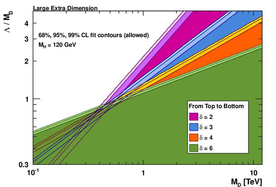
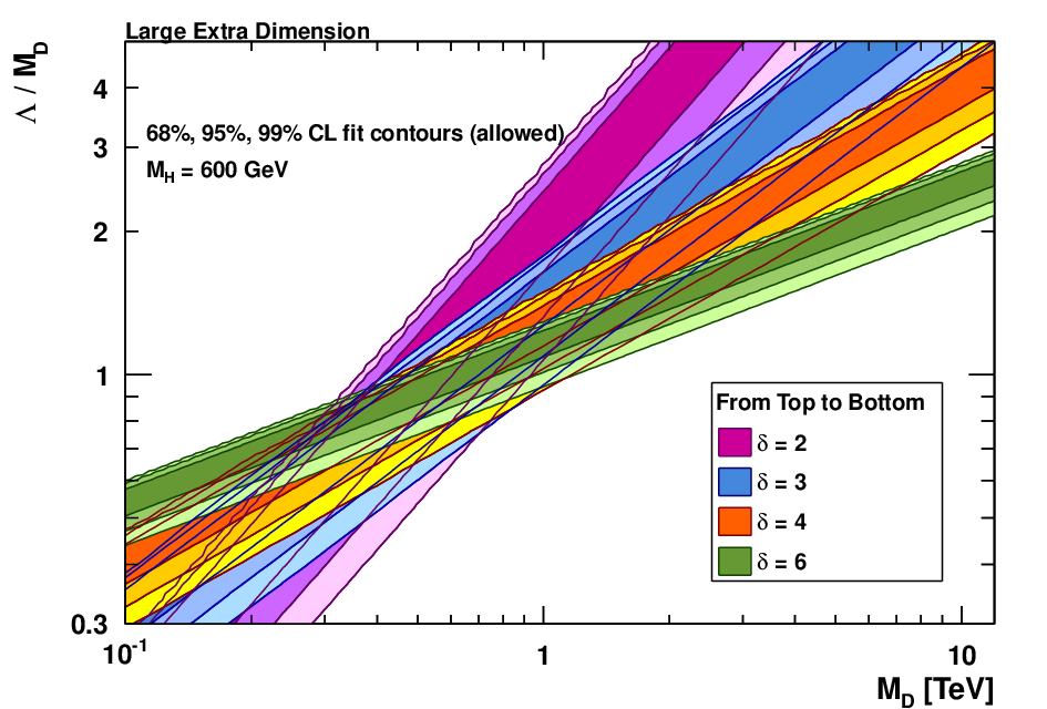
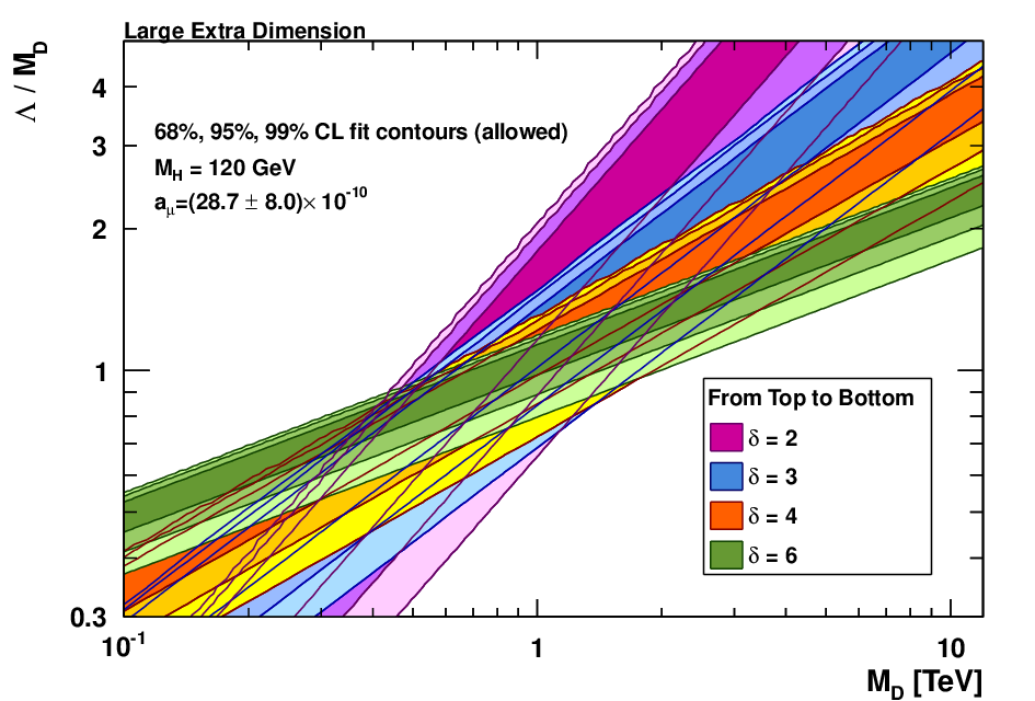
The constraints obtained for various $\delta$ in terms of 68%, 95% and 99% CL allowed regions in the ( $M_{D},\Lambda/M_{D}$ ) plane are drawn in Fig. 23 for hypothetical Higgs masses of 120 $\mathrm{Ge\kern-1.00006ptV}$ (left panel) and 600 $\mathrm{Ge\kern-1.00006ptV}$ (right panel). They show the expected behaviour of a weaker experimental constraint for rising $\delta$ where $\Lambda/M_{D}<1$ , and the opposite effect for $\Lambda/M_{D}>1$ . Owing to the significant deviation of $\overline{\varepsilon}$ from zero for $M_{H}=600\,\mathrm{Ge\kern-1.00006ptV}$ , contributions from large extra dimensions, which effectively counterweight the large negative $T$ term in the SM, are required. These heavy-Higgs scenarios are already excluded by the direct searches for $\Lambda/M_{D}<1$ (see references above).

It is possible to enhance the electroweak constraint by also including the difference between the measured [160] and predicted anomalous magnetic moment of the muon ( $a_{\mu}$ ). We use a recent evaluation of this difference, $(28.7\pm 8.0)\cdot 10^{-1}$ [58], which exhibits a $3.6\sigma$ deviation from zero (the corresponding $\tau$ -data based deviation amounts to $2.6\sigma$ ). The contribution of the large extra dimensions model to $a_{\mu}$ is also given in Ref. [155]

\delta a_{\mu}=\frac{m_{\mu}^{2}}{M_{D}^{2}}\left(\frac{\Lambda}{M_{D}}\right)^{\!\!\delta}\frac{34+11\delta}{96\,\Gamma(2+\delta/2)\pi^{2-\delta/2}}\,.

(37)

Figure 23 shows the constraints obtained for various $\delta$ from the combined usage of the electroweak precision data for $M_{H}=120\,\mathrm{Ge\kern-1.00006ptV}$ and $a_{\mu}$ . The deviation of the latter quantity from the SM value can only be accommodated by a low Planck scale, already excluded by direct experimental searches, or by a very large ultraviolet cut-off scale.

4.6 Models with universal extra dimensions

Models with flat, compactified extra dimensions where all of the SM fields are allowed to propagate into the bulk [161] are referred to as universal extra dimensions (UED) [162] (see also the review on UED phenomenology in [163] and references therein). In its minimal version one extra dimension is compactified on an $S^{1}/Z_{2}$ orbifold with two fixed points at $y=0$ and $\pi$ to obtain the SM chiral fermions from the corresponding extra dimensional fermion fields. The SM fields appear as towers of Kaluza-Klein (KK) states with tree-level masses

m^{2}_{n}=m^{2}_{0}+\frac{n^{2}}{R^{2}}\,,

(38)

where $m_{n}$ is the mass of the nth KK excitation of the SM field, $m_{0}$ is the ordinary mass of the SM particle and $R\sim\mathrm{Te\kern-1.00006ptV}^{-1}$ is the size of the extra dimension with the compactification scale $M_{{K\!K}}=R^{-1}$ . Bulk loops and brane-localised kinetic terms can lead to corrections of the KK masses of up to 20% for the KK quark and KK gluon states and of a few percent or less for the other states.

In UED models, momentum conservation in the higher dimensional space leads to a conserved KK-parity $P=(-1)^{n}$ . As a consequence, the lightest KK state is stable and could be a candidate particle for the cold dark matter in the universe. Indeed it has been shown [164, 165, 166] that the first excitation of the hypercharge gauge boson $B^{(1)}$ can account for the relic dark matter abundance of the universe if its mass is approximately 600 $\mathrm{Ge\kern-1.00006ptV}$ .²⁴²⁴ 24 If the UED is embedded into large extra dimensions of size eV^-1 accessible to gravity only, the lightest KK state could decay via KK-number violating gravitational interaction into a photon and an eV-spaced graviton tower of mass equivalent between zero and $R^{-1}$ [167]. Such a model provides a clear collider signature with two isolated photons and missing transverse energy in the final state, which has been searched for at ATLAS [168] and D0 [169]. The odd-level KK states can only be pair produced at colliders and their couplings to even number KK modes are loop suppressed. The LHC experiments should be able to detect the new KK states up to $R^{-1}\sim 1.5\>\mathrm{Te\kern-1.00006ptV}$ [170].

The SM particles that are allowed to propagate into the bulk contribute with quantum corrections to the lower energy observables. In particular, extra dimension models where only the gauge bosons are allowed to propagate into the bulk, while all other particles are confined to the SM brane, are strongly constrained by the LEP data forcing the masses of the lowest KK excitations to several TeV [171, 172], beyond the reach of possible direct detection at the LHC. KK-parity conservation in UED models forbids a direct coupling of a single KK excitation to the SM fermions and thus weakens the impact of the electroweak data. The heavy KK states can only contribute to the self energies of the gauge bosons parametrised in terms of the $S,T,U$ parameters.

The complete one-loop corrections of a given KK level $n$ of the SM fields to the gauge-boson self energies have been calculated in Ref. [173, 174]. The corrections are proportional to $m_{t}^{2}/M_{{K\!K}}^{2}$ , $M_{H}^{2}/M_{{K\!K}}^{2}$ and $M_{W}^{2}/M_{{K\!K}}^{2}$ for the top quark, Higgs, and gauge boson excitations, respectively. The contributions from top (Higgs) excitations dominate for small (large) Higgs masses. The total UED contribution corresponds to an infinite sum over $n$ , which is convergent for one extra dimension. For the leading order terms of the oblique corrections for one extra dimension we follow Refs. [173, 174] where results very similar to the present study were presented. The terms read

$\displaystyle S~$	$\displaystyle=\!\!\!\!\!\!$	$\displaystyle{4\sin\!^{2}\theta_{W}\over\alpha}$	$\displaystyle\ \left[{3g^{2}\over 4(4\pi)^{2}}\left({2\over 9}{m_{t}^{2}\over M_{{K\!K}}^{2}}\right)\zeta(2)\ +\ {g^{2}\over 4(4\pi)^{2}}\left({1\over 6}{M_{H}^{2}\over M_{{K\!K}}^{2}}\right)\zeta(2)\right]\,,$	(39)
$\displaystyle T~$	$\displaystyle=\!\!\!\!\!\!$	$\displaystyle{1\over\alpha}$	$\displaystyle\ \left[{3g^{2}\over 2(4\pi)^{2}}{m_{t}^{2}\over M_{W}^{2}}\left({2\over 3}{m_{t}^{2}\over M_{{K\!K}}^{2}}\right)\zeta(2)\ +\ {g^{2}\sin\!^{2}\theta_{W}\over(4\pi)^{2}\cos\!^{2}\theta_{W}}\left(-{5\over 12}{M_{H}^{2}\over M_{{K\!K}}^{2}}\right)\zeta(2)\right]\,,$	(40)
$\displaystyle U~$	$\displaystyle=\!\!\!\!\!\!$	$\displaystyle-{4\sin\!^{2}\theta_{W}\over\alpha}$	$\displaystyle\ \left[{g^{2}\sin\!^{2}\theta_{W}\over(4\pi)^{2}}{M_{W}^{2}\over M_{{K\!K}}^{2}}\left({1\over 6}\zeta(2)-{1\over 15}{M_{H}^{2}\over M_{{K\!K}}^{2}}\zeta(4)\right)\right]\,,$	(41)

where the $\zeta$ -functions arise from the summation over the KK tower states. Because $M_{W}^{2}\ll m_{t}^{2}\ll M_{{K\!K}}^{2}$ , the oblique parameter $T$ will dominate the electroweak precision constraints for small values of $M_{H}$ , and $U$ is negligible compared to $T$ and $S$ . Top quark and Higgs loops contribute with opposite signs to the $T$ parameter. Cancellation between these contributions is achieved for $M_{H}=\sqrt{12/5}\cdot\cot\!\theta_{W}\cdot m_{t}^{2}/M_{W}\approx 1.1\>\mathrm{Te\kern-1.00006ptV}$ . For smaller (larger) $M_{H}$ , $T$ takes positive (negative) values. The positive contribution to $T$ from the top loops also weakens the Higgs mass constraint from the global electroweak fit.²⁵²⁵ 25 This effect is similar to the cancellation of the negative SM Higgs contribution to $T$ with the positive contribution from the top sector in the littlest Higgs model (cf. Section 4.4). On the other hand, the top quark and Higgs loop contributions to $S$ have the same sign. One notices the decoupling from the SM in Eqs. (39)-(41) for small extra dimensions.

Figure 25 shows the UED prediction in the $(S,T)$ plane for various $R^{-1}$ and $M_{H}$ hypotheses. Constant values of $R^{-1}$ are depicted by the solid contour lines. The plot reproduces the UED decoupling from the SM at large compactification scales, while for small scales $T$ and $S$ can become large. The steepness of the prediction for constant $M_{H}$ in the $(S,T)$ plan reduces with increasing values of $M_{H}$ reflecting the negative (positive) sign of the Higgs contribution to $T$ ( $S$ ) in Eq. (40) (Eq. (39)). For the $T=0$ cancellation value of $M_{H}=1.1\>\mathrm{Te\kern-1.00006ptV}$ a horizontal prediction is obtained as expected (not drawn in the plot). By comparison with the electroweak data (ellipses) one notices that for large UED scales $M_{H}$ must be small and vice versa.

This behaviour is emphasised in Fig. 25, which shows the 68%, 95% and 99% CL allowed regions in the $(M_{H},R^{-1})$ plane. For large $R^{-1}$ the constraint on $M_{H}$ approaches that of the SM, while for small compactification scales significantly larger Higgs masses are allowed. The region $R^{-1}<300\>\mathrm{Ge\kern-1.00006ptV}$ and $M_{H}>750\>\mathrm{Ge\kern-1.00006ptV}$ can be excluded at 95% CL. These findings are in agreement with the results of previous publications [173, 174, 175].

It has been shown [174] that constraints derived from fits including the subleading contribution from the additional oblique parameters $X,Y,V,W$ are very similar to the results of the $S,T$ analysis. Tighter constraints can be obtained [174] when including $e^{+}e^{-}$ data from centre-of-mass energies beyond the $Z$ pole [72].

4.7 Models with warped extra dimensions

To solve the hierarchy problem, Randall and Sundrum (RS) have proposed a single, small and non-factorisable extra space dimension accessible to gravity only [176]. The geometry of this model is determined by the extra dimension confined by two three-branes. The model assumes only one fundamental mass scale, which is the ultraviolet (UV) Planck scale. The generation of the weak scale on the infrared (IR) brane from the UV brane is achieved by introducing a warp factor altering the four-dimensional Minkowski metric. The warp factor is an exponential function of the compactification radius of the extra dimension, which is small and thus precludes the extra dimension to be observed at low-scale gravity experiments. The warp factor is considered to be the source of the observed large hierarchy between Planck and weak scales in four space-time dimensions. The effective four-dimensional Planck scale is determined by a higher dimensional Planck scale and the geometry of the extra dimension.

The RS model features fundamental spin-2 KK graviton excitations, which strongly couple to the SM particles and would thus manifest themselves in form of TeV scale resonances of pairs of jets, leptons, photons, and gauge bosons in collider experiments. The scale can be reduced if either a heavy Higgs is allowed or an ultraviolet cut-off below the Planck scale is introduced. The simplest RS models contain only the SM particles and their KK excitations. These models are characterised by only two new parameters, of which one is the order-one logarithm of the warp factor, $L=kr\pi$ , where $k$ and $r$ are the dimensional curvature of the five-dimensional space-time and the compactification radius, respectively. The inverse warp factor sets the scale of the other free parameter, $M_{K\!K}=ke^{-L}$ .

In the minimal RS model, all SM fields are confined to one brane. Since in this model the unification of the gauge couplings cannot be described by an effective field theory [177] and the flavour hierarchy is not addressed alternatives have been developed. In a first extension, the SM gauge bosons are allowed to propagate into the bulk. However, $S$ and $T$ then adopt very large and negative values [178]. In following variations also the SM fermions are let to propagate into the bulk, which reduces the amount of the oblique corrections and shifting them to small, positive values. $M_{K\!K}$ then determines the lowest KK excitations of the SM fields in the bulk. The masses of the first KK gluon and photon excitations are approximately $2.5\cdot M_{K\!K}$ .

The leading contributions to the $S$ and $T$ parameters for a model with a brane-localised Higgs sector and bulk gauge and matter fields are found to be [179, 180, 181]

	$\displaystyle S$	$\displaystyle\!\!=\!\!$	$\displaystyle\frac{2\pi v^{2}}{M_{K\!K}^{2}}\left(1-\frac{1}{L}\right)\,,$		(42)
	$\displaystyle T$	$\displaystyle\!\!=\!\!$	$\displaystyle\frac{\pi v^{2}}{2\cos^{2}\theta_{W}M_{K\!K}^{2}}\left(L-\frac{1}{2L}\right)\,,$		(43)

whereas there are no contributions to $U$ . In the analysis presented here we follow the studies of Ref. [180] where similar results have been obtained.

The predicted $S$ and $T$ regions for $0.5\leq M_{K\!K}\leq 10\>\mathrm{Te\kern-1.00006ptV}$ and $5\leq L\leq 37$ are shown by the shaded (green) region on the top panel of Fig. 26. There is a large overlap with the electroweak data (ellipses). The figure also illustrates the decoupling of the RS model for large $M_{K\!K}$ .

Specific constraints from the electroweak fit on the RS model parameters in correlation with the Higgs mass are shown in the top and middle panels of Fig. 27. Large Higgs masses can be accommodated for comparatively low $M_{K\!K}$ values counteracting on the strong constraint from $T$ . A large Higgs mass is in agreement with the Higgs field being localised on the TeV brane. Assuming new physics to stabilise the hierarchy problem at a UV scale of approximately $10^{3}\>\mathrm{Te\kern-1.00006ptV}$ (corresponding to $L\approx 9$ ) would relax the $M_{K\!K}$ lower bound, cf. Fig. 27. Vice versa, one finds that small $M_{K\!K}$ values lead to an increased constraint on $L$ . Addressing the full hierarchy problem ( $L\approx 39$ ) requires the lightest KK modes to be heavy, albeit this constraint would be alleviated if the Higgs boson is heavy.

In a different approach to lowering the constraint on $M_{K\!K}$ from the $T$ parameter, one introduces a so-called custodial isospin gauge symmetry [182]. The electroweak gauge symmetry is thereby enhanced to $SU(2)_{L}\times SU(2)_{R}\times U(1)_{B-L}$ yielding a $SU(3)_{C}\times SU(2)_{L}\times SU(2)_{R}\times U(1)_{B-L}$ gauge symmetry in the bulk of the extra dimension. $SU(2)_{R}$ is then broken to $U(1)_{R}$ on the Planck brane resulting in a spontaneous breaking of $U(1)_{R}\times U(1)_{B_{L}}$ to $U(1)_{Y}$ . Consequently, the right-handed fermionic fields are promoted to doublets of this symmetry. Adding custodial isospin symmetry to the RS model leaves the $S$ parameter unchanged with respect to Eq. (42), while $T$ becomes warp-factor suppressed [182, 180]

T=-\frac{\pi v^{2}}{4\cos^{2}\theta_{W}M_{K\!K}^{2}}\frac{1}{L}\,.

(44)

The bottom plot of Fig. 26 shows the corresponding allowed region for the same parameter ranges as in the top plot. The negative $T$ oblique correction inherent in the custodial model adds to that of the SM so that only small values of $M_{H}$ are allowed.

The bottom panel of Fig. 27 shows the dependence of the two model parameters on the Higgs mass. Even though a light Higgs cannot counteract on the new physics contributions the model parameters are less constrained leading to a reduced lower bound on $M_{K\!K}$ . However, very small $M_{K\!K}$ lead to excluded Higgs masses. In addition, the strong correlation between $M_{K\!K}$ and $L$ is removed so that the Higgs mass and $M_{K\!K}$ are practically independent of $L$ . Therefore, there is no need to introduce a cut-off at a specific scale.

As an alternative to custodial symmetry, it was proposed to reduce the contribution to the $T$ parameter by also allowing the Higgs to propagate into the bulk. This leads to a preferably heavy Higgs, which can lower the bound on $M_{K\!K}$ by several TeV and therefore shift the lightest KK modes in the accessible range of the LHC [183].

In a bulk version of the Rattazzi-Zaffaroni model [184], it is assumed that the SM Yukawa hierarchy is set by UV physics and that the fundamental 5D Yukawa couplings are shined through the bulk by scalar flavor fields in agreement with flavor and CP violation constraints. Thus, a bound on the KK-scale as low as 2 TeV is allowed for specific parameter configurations [185]. However, this alternative description of flavor causes the new physics contributions to the EW parameters to be not oblique and a description by the usual $S,\,T,\,U$ formalism would be incomplete. Nonetheless, the Higgs mass may adopt values up to 200 GeV [186]. Recent hints for new physics from the Tevatron, e.g. the top quark forward-backward-asymmetry can be easily accomodated in this Flavor Triviality model.

There have been various experimental searches for high-mass graviton resonances decaying to, e.g., photon or electron pairs within the original RS model at the LHC and Tevatron [187, 188, 189, 190]. In these analyses, the invariant mass of the two-particle final states is used to set limits on the RS-graviton production cross section and lowest-level graviton mass scale. The latter one is found to be $M_{G}>\rm 1058\>GeV$ and $M_{G}>\rm 560\>GeV$ at 95% CL for $\sqrt{8\pi}k/M_{\rm Pl}=0.1$ and $\sqrt{8\pi}k/M_{\rm Pl}=0.01$ , respectively [190].

4.8 Technicolour

Elementary Higgs models provide no dynamical explanation for electroweak symmetry breaking and require a high degree of finetuning. One of the first attempts to address these shortcomings of the Standard Model were so-called technicolour (TC) models which were developed in the late 1970s [191, 192]. These models introduce a new QCD-like gauge interaction that is asymptotically free at high energies but confining at the electroweak scale. It is assumed that the technicolour gauge interaction is to be based on a $SU(N_{{\rm TC}})$ gauge group $G_{{\rm TC}}$ , where $N_{\rm TC}$ is the number of technicolours, and couples to one or more doublets of massless Dirac technifermions. In analogy to QCD, the running gauge coupling $\alpha_{{\rm TC}}$ triggers a spontaneous chiral symmetry breaking, which leads to a dynamical mass generation of the technifermions and, in addition, to a large number of massless Goldstone bosons. It is further postulated that the technifermions transform chirally under the electroweak gauge group $SU(2)\times U(1)$ so that three linear combinations of the Goldstone bosons couple to three electroweak gauge currents. It was shown in Ref. [191] that these Goldstone bosons (the so-called technipions $\pi_{T}$ ) can give mass to the electroweak gauge bosons by the usual Higgs mechanism. The properties of any remaining technipions (their corresponding quantum numbers and masses) are model dependent. Similar to the vector mesons in QCD, further technicolour resonances with masses in the TeV range are expected [36]. Direct searches for such resonances were performed at several collider experiments studying dilepton and dijet resonances [36, 193]. Model dependent 95% CL exclusion bounds on technipion and technirho masses of $80\>\mathrm{Ge\kern-1.00006ptV}<m_{\pi_{T}}<115\>\mathrm{Ge\kern-1.00006ptV}$ and $170\>\mathrm{Ge\kern-1.00006ptV}<m_{\rho_{T}}<215\>\mathrm{Ge\kern-1.00006ptV}$ were obtained.

Such simple versions of technicolour models do not explain the explicit breaking of chiral symmetries of quarks and leptons. Extended technicolour models (ETC) have been developed to address this issue by assuming that ordinary $SU(3)$ colour, $SU(N_{{\rm TC}})$ technicolour, and flavour symmetries are unified into one gauge group $G_{{\rm ETC}}$ , which allows the technifermions to couple to quarks and leptons via gauge bosons of the enlarged group. In $G_{{\rm ETC}}$ technifermions, quarks, and leptons belong to the same representations. Hence flavour, colour and technicolour can be interpreted as a subset of the ETC quantum numbers. It is assumed that the ETC gauge symmetry breaking into $SU(3)\times SU(N_{{\rm TC}})$ occurs at scales well above the TC scale of $0.1$ – $1\>\mathrm{Te\kern-1.00006ptV}$ . The broken gauge interactions give mass to the quarks and leptons by connecting them to technifermions. An introduction to technicolour models can be found, for instance, in Ref. [194].

Because technicolour is a strongly interacting theory, the oblique corrections of technicolour models cannot be calculated by ordinary perturbation theory. Two approaches are followed to address these difficulties [195]. The first approach assumes that $S$ and $T$ can be expressed as a spectral integral, which is evaluated with the use of QCD data and then extrapolated to technicolour energies [6]. The second approach is based on the relations of $S$ , $T$ , and $U$ to the coefficients of four-derivative operators in the chiral Lagrangian [10, 196]. Both approaches give consistent results for QCD-like technicolour models.

The magnitude of the radiative corrections in technicolour models increases with the number of technicolours ( $N_{{\rm TC}}$ ) and the number of techniflavours ( $N_{{\rm TF}}$ ). It is therefore justified (conservative) to choose a minimal ETC model [197], which has one technicolour generation with $N_{{\rm TC}}=2,3$ , to study the compatibility of ETC models with the electroweak data. The model chosen here contains a colour triplet of techniquarks ( $U,D$ ) with degenerate mass, and a doublet of technileptons ( $N,E$ ) with $m_{N}\leq m_{E}$ to allow for isospin splitting. The technineutrino $N$ can be of either Dirac or Majorana type. Following Refs. [6, 197, 11, 198], the oblique corrections for Dirac technineutrinos are given by

$\displaystyle S_{D}$	$\displaystyle\!\!=\!\!$	$\displaystyle 0.1\cdot({N_{\scriptscriptstyle C}}+1)\cdot N_{{\rm TC}}-\frac{N_{{\rm TC}}}{6\pi}\cdot Y\cdot\ln r\,,$	(45)
$\displaystyle T_{D}$	$\displaystyle\!\!=\!\!$	$\displaystyle\frac{N_{{\rm TC}}}{16\pi s_{0}^{2}c_{0}^{2}}\frac{m_{E}^{2}}{M_{Z}^{2}}\left(1+r-2\frac{r}{r-1}\ln r\right)\underset{\lim r\rightarrow 1}{=}\frac{N_{{\rm TC}}}{12\pi s_{0}^{2}c_{0}^{2}}\frac{\Delta m^{2}}{M_{Z}}\,,$	(46)
$\displaystyle U_{D}$	$\displaystyle\!\!=\!\!$	$\displaystyle\frac{N_{{\rm TC}}}{6\pi}\left[-\frac{5r^{2}-22r+5}{3(r-1)^{2}}+\frac{r^{3}-3r^{2}-3r+1}{(r-1)^{3}}\ln r\right]\underset{\lim r\rightarrow 1}{=}\frac{2N_{{\rm TC}}}{15\pi}\frac{\Delta m^{2}}{m_{E}^{2}}\,,$	(47)

and for Majorana technineutrinos by

$\displaystyle S_{M}$	$\displaystyle\!\!=\!\!$	$\displaystyle(0.04+0.1{N_{\scriptscriptstyle C}})\cdot N_{{\rm TC}}+\frac{N_{{\rm TC}}}{6\pi}\bigg(-\frac{r}{(1+r)^{2}}\cdot\bigg[\frac{8}{3}+\frac{3r-4r^{2}+3r^{3}}{(1-r^{2})^{2}}$	(48)
		$\displaystyle+\;2\frac{r^{6}-3r^{4}+6r^{3}-3r^{2}+1}{(1-r^{2})^{3}}\ln r\bigg]+\frac{1-r}{1+r}\ln r+\frac{3}{2}\bigg)\,,$	(48)
$\displaystyle T_{M}$	$\displaystyle\!\!=\!\!$	$\displaystyle\frac{N_{{\rm TC}}}{16\pi s_{0}^{2}c_{0}^{2}}\frac{m_{E}^{2}}{M_{Z}^{2}}\left(2-\frac{4r}{r^{2}-1}\ln r+\frac{4r}{(r+1)^{2}}\left[1-\frac{r^{2}+1}{4r}-\frac{r^{2}-r+1}{r^{2}-1}\ln r\right]\right)$	(49)
	$\displaystyle\!\!=\!\!$	$\displaystyle-\frac{N_{{\rm TC}}}{12\pi s_{0}^{2}c_{0}^{2}}\frac{\Delta m^{2}}{M_{Z}^{2}}\bigg\|_{\lim r\rightarrow 1}\,,$	(49)
$\displaystyle U_{M}$	$\displaystyle\!\!=\!\!$	$\displaystyle\frac{N_{{\rm TC}}}{6\pi}\bigg(\frac{r}{(r+1)^{2}}\left[\frac{8}{3}+\frac{3r^{3}-4r^{2}+3r}{(r^{2}-1)^{2}}-2\frac{r^{6}-3r^{4}+6r^{3}-3r^{2}+1}{(r^{2}-1)^{3}}\ln r\right]$	(50)
		$\displaystyle+\;\frac{r^{3}-3r^{2}-3r+1}{(r-1)^{3}}\ln r-\frac{13}{6}+\frac{4r}{(r-1)^{2}}\bigg)$
	$\displaystyle\!\!=\!\!$	$\displaystyle-\frac{2N_{{\rm TC}}}{15\pi}\frac{\Delta m^{2}}{m_{E}^{2}}\bigg\|_{\lim r\rightarrow 1}\,,$

where $Y=-1$ denotes the weak hypercharge of the technilepton doublet, ${N_{\scriptscriptstyle C}}=3$ defines the number of QCD colours, and $r=m_{N}^{2}/m_{E}^{2}$ . Several aspects should be noted: in the limit of $\Delta m=m_{E}-m_{N}\ll m_{E}$ , the contributions to the $T$ and $U$ parameters depend linearly on $\Delta m^{2}$ and are up to a sign-flip equivalent for the Dirac and Majorana cases. Similar formulas for $T$ and $U$ can be derived for the techniquark sector, but since $m_{U}=m_{D}$ is postulated their contributions vanish. The situation is different for the $S$ parameter where a term proportional to ${N_{\scriptscriptstyle C}}$ arises from the techniquark sector due to nonperturbative contributions [198]. The corresponding oblique corrections from the techniquark doublet ( $U,D$ ) are obtained by Eqs. (45–47) with an extra factor ${N_{\scriptscriptstyle C}}$ and the appropriate value of $Y$ .

Figure 28 shows the predicted $S$ and $T$ values for the Dirac (top) and Majorana (bottom) technineutrino cases together with the SM prediction and the electroweak data (ellipses). The shaded (green) areas correspond to the allowed parameter regions when varying the technilepton masses in the ranges²⁶²⁶ 26 The lower mass limits are determined by where the calculation of the oblique parameters can be trusted. $100\>\mathrm{Ge\kern-1.00006ptV}<m_{E}<1\>\mathrm{Te\kern-1.00006ptV}$ and $50\>\mathrm{Ge\kern-1.00006ptV}<m_{N}<m_{E}$ . For both technineutrino hypotheses, the $S$ parameter is disfavoured by the electroweak precision data as was first discussed in Refs. [6, 197]. The main difference in both figures for either model is the allowed region of $r=m_{N}^{2}/m_{E}^{2}$ , which governs the amount of isospin violation in the technilepton doublet. The sharp vertical edges for the different $N_{TC}$ regions correspond to the smallest allowed value of $r$ . Small values of $r$ , corresponding to large isospin violation in the technilepton sector, lower $S$ but increase $T$ . Even though the $T$ parameter prediction differs in sign between the Dirac and Majorana technineutrino cases, both hypotheses remain compatible with the current data. Compatible results are also found for the $U$ parameter for which, assuming $100\>\mathrm{Ge\kern-1.00006ptV}<m_{E}<500\>\mathrm{Ge\kern-1.00006ptV}$ and $50\>\mathrm{Ge\kern-1.00006ptV}<m_{N}<m_{E}$ , we find the predicted ranges

U=\begin{cases}\;[0.04,\,0.31]&\text{Dirac technineutrinos, }N_{TC}=2\\ \;[0.06,\,0.47]&\text{Dirac technineutrinos, }N_{TC}=3\\ \;[-0.01,\,0.25]&\text{Majorana technineutrinos, }N_{TC}=2\\ \;[-0.01,\,0.38]&\text{Majorana technineutrinos, }N_{TC}=3\end{cases}

(51)

where the large upper bounds in all cases arise from small values of $r$ , that is, large isospin violation.

It should be noted that the same mechanism that generates the $u,d$ and $c,s$ quark masses and their splitting is also responsible for the technifermion mass splitting. The splitting is therefore expected to be significantly smaller than the dynamically generated masses of the technifermions so that large isospin violation is disfavoured in extended technicolour models.

The $S$ incompatibility problem is present in all technicolour models that are built upon scaling up ordinary QCD. It should be noted, that allowing isospin violation in the techniquark sector leads to a further increase of the $S$ parameter and therefore an even larger incompatibility. The problem may be remedied by introducing non-QCD like technicolour gauge dynamics with a slowly evolving (or walking) gauge coupling $\alpha_{{\rm TC}}(\mu)$ over the large energy range from the TC to the ETC symmetry breaking scales. A prediction of the oblique parameters for these so-called walking technicolour models turns however out to be difficult as the QCD renormalisation group equations cannot be applied anymore. In recent years, predictions for so-called holographic walking technicolour models have been made, which indicate a possible consistency with the electroweak data [199, 200, 201, 202].

5 Conclusions and Perspectives

We have updated in this paper the results of the Standard Model fits to electroweak precision data with the Gfitter package, and revisited the electroweak constraints on several Standard Model extensions. The fit uses newest experimental results on the top quark and $W$ boson masses, and a new evaluation of the hadronic contribution to the electromagnetic fine-structure constant at $M_{Z}$ . The update of the latter parameter reduces the tension between the electroweak fit and the LEP limit on the Higgs boson mass. The LEP and Tevatron data on the direct Higgs searches have been extended by results from the 2010 Higgs searches at the LHC, using data corresponding to approximately 35 $\>{\rm pb}^{-1}$ of integrated luminosity.

From the complete fit, including the results from direct Higgs searches, we find for the mass of the Higgs boson an upper limit of 143 $\mathrm{Ge\kern-1.00006ptV}$ at 95% confidence level. This bound is alleviated to 163 $\mathrm{Ge\kern-1.00006ptV}$ when not including the direct Higgs searches (standard fit). Theoretical errors parametrising the uncertainties in the perturbative predictions of $M_{W}$ , $\sin\!^{2}\theta^{f}_{{\rm eff}}$ , and the electroweak form factors, contribute with approximately $8\>\mathrm{Ge\kern-1.00006ptV}$ to the total fit error found for $M_{H}$ in the standard fit. In a fit excluding the measurement of the top quark mass (but including the direct Higgs searches) we obtain the indirect determination $m_{t}=(177.2\pm 3.4)\>\mathrm{Ge\kern-1.00006ptV}$ , in fair agreement with the experimental world average. This error being much larger than that of the direct measurement, a reduction in the experimental error will not significantly impact the electroweak fit if the central value does not move by an unexpected amount. The experimental and theoretical effort should therefore concentrate on clarifying the relation between the measured top mass and the top pole mass used in the electroweak formalism, and the uncertainty inherent in identifying the latter mass with the former one. From the indirect determination of the mass of the $W$ boson from the complete fit we find $(80.360^{+0.014}_{-0.013})\>\mathrm{Ge\kern-1.00006ptV}$ , which is more precise and $1.6\sigma$ below the experimental world average. The indirect determination of the effective weak mixing angle from the complete fit gives $\sin\!^{2}\theta^{\ell}_{{\rm eff}}=0.23148\pm 0.00011$ , which is compatible with and more precise than the direct experimental average from the asymmetry measurements at LEP and SLD. The strong coupling constant to $\rm 3NLO$ order at the $Z$ -mass scale is found to be $\alpha_{\scriptscriptstyle S}(M_{Z}^{2})=0.1194\pm 0.0028$ , with negligible theoretical uncertainty due to the good convergence of the perturbative series at that scale.

Using the oblique parameter approach encoded in the $S,\,T,\,U$ formalism, together with a fixed Standard Model reference of $M_{H,\rm ref}=120\>$ GeV and $m_{t,\rm ref}=173\>$ GeV, we derive the experimental constraints $S=0.03\pm 0.10$ , $T=0.05\pm 0.12$ and $U=0.07\pm 0.11$ , with large correlations between the parameters. These results are used to revisit the oblique parameter constraints of the Standard Model and selected extensions, such as a fourth family, two Higgs doublet and inert Higgs models, littlest Higgs, models with large, universal or warped extra dimensions and technicolour. The constraints from the data are used to derive allowed regions in the parameter spaces of these models, where we confirm results from earlier studies. In most of these models a heavy Higgs boson can be made compatible with the electroweak precision data by adjusting the required amount of weak isospin breaking.

Given the strong performance of the LHC and its experiments, with already over 1 $\>{\rm fb}^{-1}$ integrated luminosity accumulated at the date of this paper, the present analysis might be among the last global electroweak fits working with Higgs limits only. In case of a Higgs discovery, the electroweak fit does not cease to be important. For example, as a test of the Standard Model the indirect prediction of the $W$ mass will achieve an accuracy of $11\>\mathrm{Me\kern-1.00006ptV}$ that can be confronted with experiment. The precision of the $M_{W}$ world average measurement will further improve with forthcoming Tevatron analyses and, eventually, by a measurement at the LHC with (expectantly) competitive error with the indirect determination or better. A discovery of the Higgs would also strongly impact the allowed parameter space of many new physics models via mainly the reduced flexibility of the $S$ oblique parameter and the then known amount of weak isospin violation in the electroweak Standard Model.

Acknowledgements

We are indebted to the LEP-Higgs and Tevatron-NPH working groups for providing the numerical ${\rm CL}_{\rm s+b}$ results of their direct Higgs-boson searches. It is a pleasure to thank Alexander Lenz for instructive discussions on extended fermion generations. We are grateful to Hong-Jian He und Shu-fang Su for their help on the implementation of the 2HDM oblique corrections. We thank Gian Giudice for helpful correspondance on large extra dimensions. We also thank Kenneth Lane for his helpful comments and suggestions on the technicolour studies presented here. This work is funded by the German Research Foundation (DFG) in the Collaborative Research Centre (SFB) 676 “Particles, Strings and the Early Universe” located in Hamburg. A.H. thanks the Aspen Center for Physics, which is supported by an NSF grant, for its hospitality during the finalisation of this paper.

Appendix A Oblique Parameter Formalism

Absorption of radiative corrections

Oblique corrections can generally be absorbed into the fundamental constants occurring at the tree-level of the SM. Kennedy and Lynn [203] have shown that this statement is general to all vacuum polarisation orders. In this appendix we illustrate the absorption process with some explicit examples.

The effects of oblique corrections on fermion scattering can be determined by examining how the gauge boson vacuum polarisation functions

\Pi_{ab}^{\mu\nu}(q)=\Pi_{ab}(q^{2})g^{\mu\nu}+(q^{\mu}q^{\nu}\ \textrm{terms})\,,

(52)

with $a,b=\gamma,W,Z$ , appear in the electroweak observables of interest.²⁷²⁷ 27 Owing to $U(1)_{Q}$ gauge symmetry, for the photon propagator the term $q^{\mu}q^{\nu}$ has no physical effect. For the (massive) $W$ and $Z$ propagators the terms are also negligible, since, in the interaction with light fermions, they are suppressed by the fermion mass scale compared with the $g^{\mu\nu}$ parts. From now on we shall ignore the $q^{\mu}q^{\nu}$ terms. The functions (52) have an SM and an unknown new physics component: $\Pi_{ab}^{\mu\nu}(q^{2})=\Pi_{ab}^{S\!M}(q^{2})+\delta\Pi_{ab}^{NP}(q^{2})$ .

For the $W$ and $Z$ bosons one finds the following mass corrections to the tree-level quantities²⁸²⁸ 28 Throughout this appendix the superscript $(0)$ is used to label tree-level quantities.

\begin{array}[]{rclcl}M_{W}^{2}&\!\!\equiv&M_{W}^{2}(M_{W}^{2})&\!\!=&M_{W}^{(0)\,2}+\Pi_{WW}(M_{W}^{2})\,,\\ M_{Z}^{2}&\!\!\equiv&M_{Z}^{2}(M_{Z}^{2})&\!\!=&M_{Z}^{(0)\,2}+\Pi_{ZZ}(M_{Z}^{2})\,,\end{array}

(53)

where the vacuum polarisation functions are evaluated at the poles of the propagators.

For the massless photon one has

\Pi_{\gamma\gamma}(0)=\Pi_{\gamma Z}(0)=0\,.

(54)

The impact on the electromagnetic constant $\alpha$ is obtained by taking the leading-order photon propagator plus the first-order correction. Together these yield

\frac{-ie^{2}}{q^{2}}\Big(1+i\Pi_{\gamma\gamma}(q^{2})\cdot\frac{-i}{q^{2}}\Big)\,.

(55)

The observed value of the electric charge is then found by taking the limit $q^{2}\rightarrow 0$ of this expression

4\pi\alpha_{*}(0)\equiv e_{*}^{2}(0)=\frac{g^{2}g^{\prime 2}}{g^{2}+g^{\prime 2}}\left(1+\Pi_{\gamma\gamma}^{\prime}(0)\right)\,,

(56)

where

\Pi_{\gamma\gamma}^{\prime}(0)=\frac{d\Pi_{\gamma\gamma}}{dq^{2}}\bigg|_{q^{2}=0}\,.

(57)

The weak mixing angle $s_{W}$ appears in the interactions of $Z$ bosons to fermions, and is shifted by the vacuum polarisation amplitude $\Pi_{Z\gamma}$ . The corrections change a $Z$ into a photon that decays to two fermions, with coupling strength $Qe$ , leading to the contribution

i\Pi_{Z\gamma}(q^{2})\frac{-i}{q^{2}}\cdot(ieQ)\,.

(58)

Including this correction, the $Z$ -fermion interaction takes the form

i\sqrt{g^{2}+g^{\prime 2}}\Big(T^{3}-s_{*}^{2}Q\Big)\,,

(59)

with

s_{*}^{2}(M_{Z}^{2})=s_{W}^{(0)\,2}-\frac{e}{\sqrt{g^{2}+g^{\prime 2}}}\frac{\Pi_{Z\gamma}(M_{Z}^{2})}{M_{Z}^{2}}\,,

(60)

as evaluated at $q^{2}=M_{Z}^{2}$ .

The Fermi constant, obtained from muon decays, as mediated by $W$ propagator, receives the first-order correction from the $W$ vacuum polarisation function

\frac{-ig^{2}}{q^{2}-M_{W}^{2}}\Big(1+i\Pi_{WW}(q^{2})\frac{-i}{q^{2}-M_{W}^{2}}\Big)\,.

(61)

At $q^{2}=0$ , the observed Fermi constant process shifts to

\frac{G_{F*}}{\sqrt{2}}=\frac{1}{2v^{2}}\Big(1-\frac{\Pi_{WW}(0)}{M_{W}^{2}}\Big)\,.

(62)

These examples illustrate that oblique corrections can be absorbed into the fundamental constants occurring of the SM. This conclusion is applied in the following Section.

Introduction of the S, T, U parameters

In the SM with a single Higgs doublet the relationship between the neutral and charged weak couplings is fixed by the ratio of $W$ and $Z$ boson masses

\rho\ =\ \frac{M_{W}^{2}}{M_{Z}^{2}\cos^{2}\!\theta_{\scriptscriptstyle W}}\,,

(63)

where $\rho_{0}=1$ at tree level. Generally one writes

\rho\ =\ 1+\Delta\rho\,,

(64)

where $\Delta\rho$ captures the radiative corrections to the gauge boson propagators and vertices. Inserting the first-order mass-corrections of Eqs. (53) into Eq. (63) gives

\Delta\rho\ =\ \frac{\Pi_{WW}(0)}{M_{W}^{2}}-\frac{\Pi_{ZZ}(0)}{M_{Z}^{2}}\,.

(65)

The tree-level vector and axial-vector couplings occurring in the $Z$ boson to fermion-antifermion vertex $i\overline{f}\gamma_{\mu}({g_{{\scriptscriptstyle V},f}^{(0)}}+{g_{{\scriptscriptstyle V},f}^{(0)}}\gamma_{5})fZ_{\mu}$ are given by

	$\displaystyle{g_{{\scriptscriptstyle V},f}^{(0)}}$	$\displaystyle\!\!=\!\!$	$\displaystyle I^{f}_{3}-2Q^{f}\sin^{2}\!\theta_{\scriptscriptstyle W}\,,$		(66)
	$\displaystyle{g_{{\scriptscriptstyle A},f}^{(0)}}$	$\displaystyle\!\!=\!\!$	$\displaystyle I^{f}_{3}\,,$		(67)

where $Q^{f}$ and $I^{f}_{3}$ are respectively the charge and the third component of the weak isospin. In the (minimal) SM, containing only one Higgs doublet, the weak mixing angle is defined by

\sin^{2}\!\theta_{\scriptscriptstyle W}\ =\ 1-\frac{M_{W}^{2}}{M_{Z}^{2}}\,.

(68)

Electroweak radiative corrections modify these relations, leading to the effective weak mixing angle and effective couplings

$\displaystyle\sin\!^{2}\theta^{f}_{{\rm eff}}$	$\displaystyle\ =\ \kappa^{f}_{Z}\sin^{2}\!\theta_{\scriptscriptstyle W}\,,$	(69)
$\displaystyle{g_{{\scriptscriptstyle V},f}}$	$\displaystyle\ =\ \sqrt{\rho^{f}_{Z}}\left(I^{f}_{3}-2Q^{f}\sin\!^{2}\theta^{f}_{{\rm eff}}\right)\,,$	(70)
$\displaystyle{g_{{\scriptscriptstyle A},f}}$	$\displaystyle\ =\ \sqrt{\rho^{f}_{Z}}I^{f}_{3}\,,$	(71)

where the radiative corrections are absorbed in the form factors $\kappa^{f}_{Z}=1+\Delta\kappa^{f}_{Z}$ and $\rho^{f}_{Z}=1+\Delta\rho^{f}_{Z}$ .

Electroweak unification leads to a relation between weak and electromagnetic couplings, which at tree level reads

{G_{\scriptscriptstyle F}}\ =\ \frac{\pi\alpha}{\sqrt{2}\left(M_{W}^{(0)}\right)^{2}\left(1-\frac{(M^{(0)}_{W})^{2}}{M_{Z}^{2}}\right)}\,.

(72)

The radiative corrections are parametrised by multiplying the r.h.s. of Eq. (72) with the form factor $(1-\Delta r)^{-1}$ . Using Eq. (68) and resolving for $M_{W}$ gives

M_{W}^{2}\ =\ \frac{M_{Z}^{2}}{2}\left(1+\sqrt{1-\frac{\sqrt{8}\,\pi\alpha(1+\Delta r)}{{G_{\scriptscriptstyle F}}{M_{Z}^{2}}}}\right)\,.

(73)

An extra correction is required for the $Z\rightarrow b\overline{b}$ decay vertex. The bottom quark is the only fermion that receives unsuppressed vertex corrections from the top quark. These corrections turn out to be significant – at the level of $G_{F}m_{t}^{2}$ – and must be accounted for. The vector and axial couplings receive an extra contribution $\varepsilon_{b}$

{g_{{\scriptscriptstyle V},b}}=-\frac{1}{2}\sqrt{\rho^{b}_{Z}}\left(1-\frac{4}{3}\sin^{2}\!\theta_{\rm eff}+\varepsilon_{b}\right)\ \ \textrm{and}\quad{g_{{\scriptscriptstyle A},b}}=-\frac{1}{2}\sqrt{\rho^{b}_{Z}}\left(1+\varepsilon_{b}\right)\,,

(74)

where $\varepsilon_{b}$ contains all top-quark induced vertex corrections.

The entire dependence of the electroweak theory on $m_{t}$ and $M_{H}$ , arising from one-loop diagrams and higher, only enters through the four parameters $\Delta\kappa$ , $\Delta\rho$ , $\Delta r$ , and $\varepsilon_{b}$ . The quantities $\Delta\kappa$ , $\Delta\rho$ , and $\Delta r_{W}$ are mostly sensitive to the absolute mass splittings between different weak-isospin partners. In practise this means the mass differences between the top and bottom quarks, and the $Z$ and $W$ bosons. For example, the dominant contributions to $\Delta\rho$ are [203]

$\displaystyle\Delta\rho_{t}$	$\displaystyle\!\!=\!\!$	$\displaystyle\frac{3G_{F}}{8\sqrt{2}\pi^{2}}\left[m_{t}^{2}+m_{b}^{2}-\frac{2m_{t}^{2}m_{b}^{2}}{m_{t}^{2}-m_{b}^{2}}\ln\left(\frac{m_{t}^{2}}{m_{b}^{2}}\right)\right]\,\ \geq\,\ \frac{3G_{F}}{8\sqrt{2}\pi^{2}}(m_{t}-m_{b})^{2}$
	$\displaystyle\!\!\longrightarrow\!\!$	$\displaystyle\frac{3G_{F}m_{t}^{2}}{8\sqrt{2}\pi^{2}}\,,\ \ \textrm{as}\quad m_{t}^{2}\gg m_{b}^{2}\,,$
$\displaystyle\Delta\rho_{H}$	$\displaystyle\!\!=\!\!$	$\displaystyle\frac{3G_{F}}{8\sqrt{2}\pi^{2}}\left[M_{W}^{2}\ln\left(\frac{M_{H}^{2}}{M_{W}^{2}}\right)-M_{Z}^{2}\ln\left(\frac{M_{H}^{2}}{M_{Z}^{2}}\right)\right]\,,$	(75)

exhibiting a quadratic dependence on the top mass, and a logarithmic dependence on the Higgs mass. Since $M_{H}>M_{Z}>M_{W}$ , $\rho_{H}$ is negative.

Ignoring terms proportional to $\ln{m_{t}/M_{Z}}$ and vertex corrections, which do not contain sizable terms containing $M_{H}$ and $m_{t}$ , the parameters on one-loop level can can be written as [204]:

$\displaystyle\Delta\rho$	$\displaystyle\!\!=\!\!$	$\displaystyle\frac{3G_{F}M_{W}^{2}}{8\sqrt{2}\pi^{2}}\left[\frac{m_{t}^{2}}{M_{W}^{2}}-\frac{\sin^{2}\!\theta_{W}}{\cos^{2}\!\theta_{W}}\left(\ln{\frac{M_{H}^{2}}{M_{W}^{2}}}-\frac{5}{6}\right)+...\right]$
$\displaystyle\Delta\kappa$	$\displaystyle\!\!=\!\!$	$\displaystyle\frac{3G_{F}M_{W}^{2}}{8\sqrt{2}\pi^{2}}\left[\frac{m_{t}^{2}}{M_{W}^{2}}\frac{\cos^{2}\!\theta_{W}}{\sin^{2}\!\theta_{W}}-\frac{10}{9}\left(\ln{\frac{M_{H}^{2}}{M_{W}^{2}}}-\frac{5}{6}\right)+...\right]$	(76)
$\displaystyle\Delta r_{W}$	$\displaystyle\!\!=\!\!$	$\displaystyle\frac{3G_{F}M_{W}^{2}}{8\sqrt{2}\pi^{2}}\left[-\frac{m_{t}^{2}}{M_{W}^{2}}\frac{\cos^{2}\!\theta_{W}}{\sin^{2}\!\theta_{W}}+\frac{11}{3}\left(\ln{\frac{M_{H}^{2}}{M_{W}^{2}}}-\frac{5}{6}\right)+...\right]$
$\displaystyle\varepsilon_{b}$	$\displaystyle\!\!=\!\!$	$\displaystyle-\frac{G_{F}m_{t}^{2}}{4\sqrt{2}\pi^{2}}+\ldots\,.$

All quantities are dominated by terms of $G_{F}m_{t}^{2}$ . Considering this term only, $\Delta k$ , $\Delta\rho$ , $\Delta r_{W}$ are related as follows

\Delta r_{W}=\frac{c^{2}-s^{2}}{s^{2}}\Delta k=-\frac{c^{2}}{s^{2}}\Delta\rho\,.

(77)

Restoring the $\ln\!\frac{m_{t}}{m_{z}}$ terms, the $\varepsilon_{1,2,3}$ parameters defined in Eqs. (8–10) on page 8 are given by

$\displaystyle\varepsilon_{1}$	$\displaystyle\!\!=\!\!$	$\displaystyle\frac{3G_{F}M_{W}^{2}}{8\sqrt{2}\pi^{2}}\left[\frac{m_{t}^{2}}{M_{W}^{2}}-\frac{\sin^{2}\!\theta_{W}}{\cos^{2}\!\theta_{W}}\left(\ln{\frac{M_{H}^{2}}{M_{W}^{2}}}-\frac{5}{6}\right)+...\right]$
$\displaystyle\varepsilon_{2}$	$\displaystyle\!\!=\!\!$	$\displaystyle\frac{3G_{F}M_{W}^{2}}{2\sqrt{2}\pi^{2}}\ln\frac{m_{t}}{M_{Z}}+...$	(78)
$\displaystyle\varepsilon_{3}$	$\displaystyle\!\!=\!\!$	$\displaystyle\frac{3G_{F}M_{W}^{2}}{8\sqrt{2}\pi^{2}}\left[\frac{2}{9}\left(\ln{\frac{M_{H}^{2}}{M_{W}^{2}}}-\frac{5}{6}\right)-\frac{4}{9}\ln{\frac{m_{t}}{M_{Z}}}+...\right]\,.$

The SM subtraction results in the parameter set $\hat{\varepsilon}$ . In terms of propagator functions one has [36]

$\displaystyle\hat{\varepsilon_{1}}$	$\displaystyle\!\!=\!\!$	$\displaystyle\frac{\Pi_{WW}^{NP}(0)}{M_{W}^{2}}-\frac{\Pi_{ZZ}^{NP}(0)}{M_{Z}^{2}}\,,$
$\displaystyle\frac{\hat{\varepsilon_{3}}}{c^{2}}$	$\displaystyle\!\!=\!\!$	$\displaystyle\frac{\Pi_{ZZ}^{NP}(M_{Z}^{2})-\Pi_{ZZ}^{NP}(0)}{M_{Z}^{2}}-\Pi_{\gamma\gamma}^{\prime\,NP}(0)-\Big(\frac{c^{2}-s^{2}}{cs}\Big)\frac{\Pi_{Z\gamma}^{NP}(M_{Z}^{2})}{M_{Z}^{2}}\,,$
$\displaystyle\hat{\varepsilon_{3}}\!-\!\hat{\varepsilon_{2}}$	$\displaystyle\!\!=\!\!$	$\displaystyle\frac{\Pi_{WW}^{NP}(M_{W}^{2})-\Pi_{WW}^{NP}(0)}{M_{W}^{2}}-\Pi_{\gamma\gamma}^{\prime\,NP}(0)-\Big(\frac{c}{s}\Big)\frac{\Pi_{Z\gamma}^{NP}(M_{Z}^{2})}{M_{Z}^{2}}\,.$	(79)

Equivalently, contributions to $\hat{\varepsilon}_{b}$ are the NP vertex correction to $Z\rightarrow b\overline{b}$ . The $S,\,T,\,U$ parameters expressed in terms of the $\hat{\varepsilon}$ parameters read

S=\frac{4s^{2}\hat{\varepsilon}_{3}}{\alpha(M_{Z}^{2})}\,,\hskip 14.22636ptT=\frac{\hat{\varepsilon}_{1}}{\alpha(M_{Z}^{2})}\,,\hskip 14.22636ptU=\frac{-4s^{2}\hat{\varepsilon}_{2}}{\alpha(M_{Z}^{2})}\,.

(80)

References

[1] Particle Data Group, G. Cowan, J. Phys. G37, 075021 (2010).
[2] Gfitter Group, H. Flaecher et al., Eur. Phys. J. C60, 543 (2009), [0811.0009], Erratum-ibid. C71 (2011) 1718.
[3] LEP Electroweak Working Group (LEP EWWG), Status of July 2010,
http://lepewwg.web.cern.ch/LEPEWWG/.
[4] J. Erler and P. Langacker (in: Review for Particle Data Group), J. Phys. G37, 075021 (2010).
[5] M. E. Peskin and T. Takeuchi, Phys. Rev. Lett. 65, 964 (1990).
[6] M. E. Peskin and T. Takeuchi, Phys. Rev. D46, 381 (1992).
[7] W. J. Marciano and J. L. Rosner, Phys. Rev. Lett. 65, 2963 (1990).
[8] D. C. Kennedy and P. Langacker, Phys. Rev. Lett. 65, 2967 (1990).
[9] D. C. Kennedy and P. Langacker, Phys. Rev. D44, 1591 (1991), Erratum-ibid. 66, 395 (1991).
[10] B. Holdom and J. Terning, Phys. Lett. B247, 88 (1990).
[11] M. Golden and L. Randall, Nucl. Phys. B361, 3 (1991).
[12] G. Altarelli and R. Barbieri, Phys. Lett. B253, 161 (1991).
[13] G. Altarelli, R. Barbieri and S. Jadach, Nucl. Phys. B369, 3 (1992), Erratum-ibid. B376, 444 (1992).
[14] M. Awramik, M. Czakon, A. Freitas and G. Weiglein, Phys. Rev. D69, 053006 (2004), [hep-ph/0311148].
[15] M. Awramik, M. Czakon, A. Freitas and G. Weiglein, Phys. Rev. Lett. 93, 201805 (2004), [hep-ph/0407317].
[16] M. Awramik, M. Czakon and A. Freitas, JHEP 11, 048 (2006), [hep-ph/0608099].
[17] K. Hagiwara, S. Matsumoto, D. Haidt and C. Kim, Z. Phys. C64, 559 (1994), [hep-ph/9409380], Order of authors changed in journal.
[18] K. Hagiwara, Ann. Rev. Nucl. Part. Sci. 48, 463 (1998).
[19] G.-C. Cho and K. Hagiwara, Nucl.Phys. B574, 623 (2000), [hep-ph/9912260].
[20] G.-C. Cho, K. Hagiwara, Y. Matsumoto and D. Nomura, 1104.1769, * Temporary entry *.
[21] A. A. Akhundov, D. Y. Bardin and T. Riemann, Nucl. Phys. B276, 1 (1986).
[22] A. B. Arbuzov et al., Comput. Phys. Commun. 174, 728 (2006), [hep-ph/0507146].
[23] D. Y. Bardin, S. Riemann and T. Riemann, Z. Phys. C32, 121 (1986).
[24] R. Barbieri, M. Beccaria, P. Ciafaloni, G. Curci and A. Vicere, Nucl. Phys. B409, 105 (1993).
[25] J. Fleischer, O. V. Tarasov and F. Jegerlehner, Phys. Lett. B319, 249 (1993).
[26] D. Y. Bardin et al., Comput. Phys. Commun. 133, 229 (2001), [hep-ph/9908433].
[27] G. Degrassi, S. Fanchiotti, F. Feruglio, B. P. Gambino and A. Vicini, Phys. Lett. B350, 75 (1995), [hep-ph/9412380].
[28] G. Degrassi, F. Feruglio, A. Vicini, S. Fanchiotti and P. Gambino, hep-ph/9507286.
[29] G. Degrassi, P. Gambino and A. Vicini, Phys. Lett. B383, 219 (1996), [hep-ph/9603374].
[30] G. Degrassi and P. Gambino, Nucl. Phys. B567, 3 (2000), [hep-ph/9905472].
[31] Electroweak working group, D. Y. Bardin et al., hep-ph/9709229, Prepared for Workshop Group on Precision Calculations for the Z Resonance (2nd meeting held Mar 31, 3rd meeting held Jun 13), Geneva, Switzerland, 14 Jan 1994, CERN-YELLOW-95-03A.
[32] D. Y. Bardin and G. Passarino, The standard model in the making: Precision study of the electroweak interactions, Oxford, UK: Clarendon (1999) 685 p.
[33] B. A. Kniehl, Nucl. Phys. B347, 86 (1990).
[34] M. Goebel, PhD thesis, University Hamburg, 2011.
[35] P. A. Baikov, K. G. Chetyrkin and J. H. Kuhn, Phys. Rev. Lett. 101, 012002 (2008), [0801.1821].
[36] Particle Data Group, K. Nakamura et al., J. Phys. G37, 075021 (2010).
[37] A. Hoecker, H. Lacker, S. Laplace and F. Le Diberder, Eur. Phys. J. C21, 225 (2001), [hep-ph/0104062].
[38] CKMfitter Group, J. Charles et al., Eur. Phys. J. C41, 1 (2005), [hep-ph/0406184].
[39] The ALEPH, DELPHI, L3, OPAL, SLD Collaborations, the LEP Electroweak Working Group, the SLD Electroweak and Heavy Flavour Working Groups, Phys. Rept. 427, 257 (2006), [hep-ex/0509008].
[40] CDF Collaboration, D. E. Acosta et al., Phys. Rev. D71, 052002 (2005), [hep-ex/0411059].
[41] D0 Collaboration, V. Abazov et al., Phys. Rev. Lett. 101, 191801 (2008), [0804.3220].
[42] NuTeV Collaboration, G. P. Zeller et al., Phys. Rev. Lett. 88, 091802 (2002), [hep-ex/0110059].
[43] K. J. Eskola and H. Paukkunen, JHEP 06, 008 (2006), [hep-ph/0603155].
[44] S. Davidson, S. Forte, P. Gambino, N. Rius and A. Strumia, JHEP 02, 037 (2002), [hep-ph/0112302].
[45] K. S. McFarland and S.-O. Moch, hep-ph/0306052, Proceedings of Mini-Workshop on Electroweak Precision Data and the Higgs Mass, Zeuthen, Germany, 28 Feb–1 Mar, 2003.
[46] Tevatron Electroweak Working Group and CDF and D0 Collaborations, 0908.1374.
[47] Tevatron Electroweak Working Group, 1003.2826.
[48] CDF and D0 Collaborations, 1007.3178.
[49] P. Skands and D. Wicke, Eur. Phys. J. C52, 133 (2007), [hep-ph/0703081].
[50] D. Wicke and P. Z. Skands, 0807.3248.
[51] A. H. Hoang, A. Jain, I. Scimemi and I. W. Stewart, 0803.4214.
[52] A. H. Hoang and I. W. Stewart, 0808.0222.
[53] U. Langenfeld, S. Moch and P. Uwer, Phys. Rev. D80, 054009 (2009), [0906.5273].
[54] K. Melnikov and T. v. Ritbergen, Phys. Lett. B482, 99 (2000), [hep-ph/9912391].
[55] D0 Collaboration, V. M. Abazov et al., 1101.0124.
[56] D0 Collaboration, V. M. Abazov et al., 1104.2887.
[57] N. Kidonakis, Phys. Rev. D82, 114030 (2010), [1009.4935].
[58] M. Davier, A. Hoecker, B. Malaescu and Z. Zhang, Eur. Phys. J. C71, 1515 (2011), [1010.4180].
[59] K. Hagiwara, A. D. Martin, D. Nomura and T. Teubner, Phys. Lett. B649, 173 (2007), [hep-ph/0611102].
[60] The ALEPH, DELPHI, L3 and OPAL Collaborations, and LEP Working Group for Higgs Boson Searches, R. Barate et al., Phys. Lett. B565, 61 (2003), [hep-ex/0306033].
[61] CDF and D0 Collaborations, 1007.4587.
[62] CDF and D0 Collaborations, T. Aaltonen et al., 1103.3233.
[63] ATLAS Collaboration, G. Aad et al., 1106.2748, CERN-PH-EP-2011-076 (2011).
[64] CMS Collaboration, S. Chatrchyan et al., Phys. Lett. B699, 25 (2011), [1102.5429].
[65] G. Cowan, K. Cranmer, E. Gross and O. Vitells, Eur. Phys. J. C71, 1554 (2011), [1007.1727].
[66] K. Hagiwara, R. Liao, A. D. Martin, D. Nomura and T. Teubner, J. Phys. G38, 085003 (2011), [1105.3149].
[67] Gfitter Group, M. Baak et al., Updated results at: http://cern.ch/gfitter.
[68] G. Altarelli, R. Barbieri and F. Caravaglios, Nucl. Phys. B405, 3 (1993).
[69] G. Altarelli, R. Barbieri and F. Caravaglios, Int. J. Mod. Phys. A13, 1031 (1998), [hep-ph/9712368].
[70] C. P. Burgess, S. Godfrey, H. Konig, D. London and I. Maksymyk, Phys. Rev. D49, 6115 (1994), [hep-ph/9312291].
[71] C. P. Burgess, S. Godfrey, H. Konig, D. London and I. Maksymyk, Phys. Lett. B326, 276 (1994), [hep-ph/9307337].
[72] R. Barbieri, A. Pomarol, R. Rattazzi and A. Strumia, Nucl. Phys. B703, 127 (2004), [hep-ph/0405040].
[73] C. P. Burgess, Pramana 45, S47 (1995), [hep-ph/9411257].
[74] A. Arhrib and W.-S. Hou, Eur. Phys. J. C27, 555 (2003), [hep-ph/0211267].
[75] W.-S. Hou, M. Nagashima and A. Soddu, Phys. Rev. D76, 016004 (2007), [hep-ph/0610385].
[76] W.-S. Hou, M. Nagashima and A. Soddu, Phys. Rev. D72, 115007 (2005), [hep-ph/0508237].
[77] W.-S. Hou, H.-n. Li, S. Mishima and M. Nagashima, Phys. Rev. Lett. 98, 131801 (2007), [hep-ph/0611107].
[78] A. Soni, A. K. Alok, A. Giri, R. Mohanta and S. Nandi, Phys. Lett. B683, 302 (2010), [0807.1971].
[79] F. J. Botella, G. C. Branco and M. Nebot, J. Phys. Conf. Ser. 171, 012058 (2009).
[80] O. Eberhardt, A. Lenz and J. Rohrwild, Phys. Rev. D82, 095006 (2010), [1005.3505].
[81] M. Bobrowski, A. Lenz, J. Riedl and J. Rohrwild, Phys. Rev. D79, 113006 (2009), [0902.4883].
[82] A. Soni, A. K. Alok, A. Giri, R. Mohanta and S. Nandi, Phys. Rev. D82, 033009 (2010), [1002.0595].
[83] A. J. Buras et al., JHEP 09, 106 (2010), [1002.2126].
[84] H. Lacker and A. Menzel, JHEP 07, 006 (2010), [1003.4532].
[85] J. Erler and P. Langacker, Phys. Rev. Lett. 105, 031801 (2010), [1003.3211].
[86] P. H. Frampton, P. Q. Hung and M. Sher, Phys. Rept. 330, 263 (2000), [hep-ph/9903387].
[87] B. Holdom, Phys. Rev. D54, 721 (1996), [hep-ph/9602248].
[88] B. Holdom, JHEP 0608, 076 (2006), [hep-ph/0606146].
[89] H.-J. He, N. Polonsky and S.-f. Su, Phys. Rev. D64, 053004 (2001), [hep-ph/0102144].
[90] G. D. Kribs, T. Plehn, M. Spannowsky and T. M. P. Tait, Phys. Rev. D76, 075016 (2007), [0706.3718].
[91] V. A. Novikov, L. B. Okun, A. N. Rozanov and M. I. Vysotsky, JETP Lett. 76, 127 (2002), [hep-ph/0203132].
[92] M. S. Chanowitz, Phys. Rev. D, 035018 (2010), [1007.0043].
[93] M. S. Chanowitz, Phys. Rev. D79, 113008 (2009), [0904.3570].
[94] CMS Collaboration, S. Chatrchyan et al., Phys. Lett. B701, 204 (2011), [1102.4746].
[95] CDF Collaboration, J. Conway et al., CDF/PUB/TOP/PUBLIC/10395 (2011).
[96] CDF Collaboration, T. Aaltonen et al., 1101.5728.
[97] C. J. Flacco, D. Whiteson and M. Kelly, 1101.4976.
[98] C. J. Flacco, D. Whiteson, T. M. P. Tait and S. Bar-Shalom, Phys. Rev. Lett. 105, 111801 (2010), [1005.1077].
[99] L3 Collaboration, P. Achard et al., Phys. Lett. B517, 75 (2001), [hep-ex/0107015].
[100] M. Hashimoto, Phys. Rev. D81, 075023 (2010), [1001.4335].
[101] J. R. Espinosa, G. F. Giudice and A. Riotto, JCAP 0805, 002 (2008), [0710.2484].
[102] J. Ellis, J. Espinosa, G. Giudice, A. Hoecker and A. Riotto, Phys.Lett. B679, 369 (2009), [0906.0954].
[103] CDF and D0 Collaborations, T. Aaltonen et al., 1005.3216.
[104] H. E. Haber, G. L. Kane and T. Sterling, Nucl. Phys. B161, 493 (1979).
[105] H. E. Haber and D. O’Neil, Phys. Rev. D74, 015018 (2006), [hep-ph/0602242].
[106] S. Davidson and H. E. Haber, Phys. Rev. D72, 035004 (2005), [hep-ph/0504050].
[107] J. M. Cline and P.-A. Lemieux, Phys. Rev. D55, 3873 (1997), [hep-ph/9609240].
[108] J. F. Gunion, H. E. Haber, G. L. Kane and S. Dawson, hep-ph/9302272.
[109] L. F. Abbott, P. Sikivie and M. B. Wise, Phys. Rev. D21, 1393 (1980).
[110] O. Deschamps et al., Phys. Rev. D82, 073012 (2009), [0907.5135].
[111] ALEPH Collaboration, A. Heister et al., Phys. Lett. B543, 1 (2002), [hep-ex/0207054].
[112] DELPHI Collaboration, P. Abreu et al., Phys.Lett. B525, 17 (2002), [hep-ex/0201023].
[113] L3 Collaboration, P. Achard et al., Phys. Lett. B575, 208 (2003), [hep-ex/0309056].
[114] OPAL Collaboration, G. Abbiendi et al., Eur. Phys. J. C7, 407 (1999), [hep-ex/9811025].
[115] LEP Higgs Working Group for Higgs boson searches, hep-ex/0107031.
[116] H. E. Haber, hep-ph/9306207.
[117] H. E. Haber and H. E. Logan, Phys. Rev. D62, 015011 (2000), [hep-ph/9909335].
[118] C. D. Froggatt, R. G. Moorhouse and I. G. Knowles, Phys. Rev. D45, 2471 (1992).
[119] R. Barbieri, L. J. Hall and V. S. Rychkov, Phys. Rev. D74, 015007 (2006), [hep-ph/0603188].
[120] N. G. Deshpande and E. Ma, Phys. Rev. D18, 2574 (1978).
[121] L. Lopez Honorez, E. Nezri, J. F. Oliver and M. H. G. Tytgat, JCAP 0702, 028 (2007), [hep-ph/0612275].
[122] M. Gustafsson, E. Lundstrom, L. Bergstrom and J. Edsjo, Phys. Rev. Lett. 99, 041301 (2007), [astro-ph/0703512].
[123] E. Lundstrom, M. Gustafsson and J. Edsjo, Phys. Rev. D79, 035013 (2009), [0810.3924].
[124] T. Hambye, F. S. Ling, L. Lopez Honorez and J. Rocher, JHEP 07, 090 (2009), [0903.4010].
[125] S. Andreas, M. H. Tytgat and Q. Swillens, JCAP 0904, 004 (2009), [0901.1750].
[126] E. M. Dolle and S. Su, Phys. Rev. D80, 055012 (2009), [0906.1609].
[127] L. Lopez Honorez and C. E. Yaguna, JHEP 09, 046 (2010), [1003.3125].
[128] L. Lopez Honorez and C. E. Yaguna, JCAP 1101, 002 (2011), [1011.1411].
[129] D. B. Kaplan and H. Georgi, Phys. Lett. B136, 183 (1984).
[130] D. B. Kaplan, H. Georgi and S. Dimopoulos, Phys. Lett. B136, 187 (1984).
[131] H. Georgi, D. B. Kaplan and P. Galison, Phys. Lett. B143, 152 (1984).
[132] H. Georgi and D. B. Kaplan, Phys. Lett. B145, 216 (1984).
[133] N. Arkani-Hamed, A. G. Cohen and H. Georgi, Phys. Lett. B513, 232 (2001), [hep-ph/0105239].
[134] N. Arkani-Hamed, A. G. Cohen, T. Gregoire and J. G. Wacker, JHEP 08, 020 (2002), [hep-ph/0202089].
[135] N. Arkani-Hamed, A. G. Cohen, E. Katz and A. E. Nelson, JHEP 07, 034 (2002), [hep-ph/0206021].
[136] C. Csaki, J. Hubisz, G. D. Kribs, P. Meade and J. Terning, Phys. Rev. D68, 035009 (2003), [hep-ph/0303236].
[137] M. Perelstein, M. E. Peskin and A. Pierce, Phys. Rev. D69, 075002 (2004), [hep-ph/0310039].
[138] C. Csaki, J. Hubisz, G. D. Kribs, P. Meade and J. Terning, Phys. Rev. D67, 115002 (2003), [hep-ph/0211124].
[139] J. L. Hewett, F. J. Petriello and T. G. Rizzo, JHEP 10, 062 (2003), [hep-ph/0211218].
[140] T. Han, H. E. Logan, B. McElrath and L.-T. Wang, Phys. Rev. D67, 095004 (2003), [hep-ph/0301040].
[141] H.-C. Cheng and I. Low, JHEP 09, 051 (2003), [hep-ph/0308199].
[142] H.-C. Cheng and I. Low, JHEP 08, 061 (2004), [hep-ph/0405243].
[143] J. Hubisz and P. Meade, Phys. Rev. D71, 035016 (2005), [hep-ph/0411264].
[144] J. Hubisz, P. Meade, A. Noble and M. Perelstein, JHEP 01, 135 (2006), [hep-ph/0506042].
[145] M. Asano, S. Matsumoto, N. Okada and Y. Okada, Phys. Rev. D75, 063506 (2007), [hep-ph/0602157].
[146] N. Arkani-Hamed, S. Dimopoulos and G. R. Dvali, Phys. Lett. B429, 263 (1998), [hep-ph/9803315].
[147] I. Antoniadis, N. Arkani-Hamed, S. Dimopoulos and G. R. Dvali, Phys. Lett. B436, 257 (1998), [hep-ph/9804398].
[148] D. J. Kapner et al., Phys. Rev. Lett. 98, 021101 (2007), [hep-ph/0611184].
[149] Particle Data Group, G. F. Giudice and J. D. Wells, J. Phys. G37, 075021 (2010).
[150] S. Hannestad and G. G. Raffelt, Phys. Rev. Lett. 88, 071301 (2002), [hep-ph/0110067].
[151] G. F. Giudice, R. Rattazzi and J. D. Wells, Nucl. Phys. B544, 3 (1999), [hep-ph/9811291].
[152] T. Han, J. D. Lykken and R.-J. Zhang, Phys. Rev. D59, 105006 (1999), [hep-ph/9811350].
[153] J. L. Hewett, Phys. Rev. Lett. 82, 4765 (1999), [hep-ph/9811356].
[154] G. F. Giudice and A. Strumia, Nucl. Phys. B663, 377 (2003), [hep-ph/0301232].
[155] R. Contino, L. Pilo, R. Rattazzi and A. Strumia, JHEP 06, 005 (2001), [hep-ph/0103104].
[156] G. Landsberg, 0808.1867.
[157] S. Ask, hep-ex/0410004.
[158] CMS Collaboration, S. Chatrchyan et al., JHEP 05, 085 (2011), [1103.4279].
[159] ATLAS Collaboration, G. Aad et al., 1106.5327, CERN-PH-EP-2011-090 (2011).
[160] Muon G-2 Collaboration, G. W. Bennett et al., Phys. Rev. D73, 072003 (2006), [hep-ex/0602035].
[161] I. Antoniadis, Phys.Lett. B246, 377 (1990).
[162] T. Appelquist, H.-C. Cheng and B. A. Dobrescu, Phys. Rev. D64, 035002 (2001), [hep-ph/0012100].
[163] D. Hooper and S. Profumo, Phys. Rept. 453, 29 (2007), [hep-ph/0701197].
[164] G. Servant and T. M. Tait, Nucl.Phys. B650, 391 (2003), [hep-ph/0206071].
[165] F. Burnell and G. D. Kribs, Phys. Rev. D73, 015001 (2006), [hep-ph/0509118].
[166] K. Kong and K. T. Matchev, JHEP 0601, 038 (2006), [hep-ph/0509119].
[167] C. Macesanu, C. D. McMullen and S. Nandi, Phys. Lett. B546, 253 (2002), [hep-ph/0207269].
[168] ATLAS Collaboration, G. Aad et al., Phys. Rev. Lett. 106, 121803 (2011), [1012.4272].
[169] D0 Collaboration, V. M. Abazov et al., Phys. Rev. Lett. 105, 221802 (2010), [1008.2133].
[170] H.-C. Cheng, K. T. Matchev and M. Schmaltz, Phys. Rev. D66, 056006 (2002), [hep-ph/0205314].
[171] M. Masip and A. Pomarol, Phys. Rev. D60, 096005 (1999), [hep-ph/9902467].
[172] T. G. Rizzo and J. D. Wells, Phys. Rev. D61, 016007 (2000), [hep-ph/9906234].
[173] T. Appelquist and H.-U. Yee, Phys. Rev. D67, 055002 (2003), [hep-ph/0211023].
[174] I. Gogoladze and C. Macesanu, Phys. Rev. D74, 093012 (2006), [hep-ph/0605207].
[175] T. Flacke, D. Hooper and J. March-Russell, Phys. Rev. D73, 095002 (2006), [hep-ph/0509352], Erratum-ibid. D74, 019902 (2006).
[176] L. Randall and R. Sundrum, Phys. Rev. Lett. 83, 3370 (1999), [hep-ph/9905221].
[177] K. Agashe, A. Delgado and R. Sundrum, Ann. Phys. 304, 145 (2003), [hep-ph/0212028].
[178] C. Csaki, J. Erlich and J. Terning, Phys. Rev. D66, 064021 (2002), [hep-ph/0203034].
[179] A. Delgado and A. Falkowski, JHEP 05, 097 (2007), [hep-ph/0702234].
[180] S. Casagrande, F. Goertz, U. Haisch, M. Neubert and T. Pfoh, JHEP 0810, 094 (2008), [0807.4937].
[181] M. S. Carena, A. Delgado, E. Ponton, T. M. P. Tait and C. E. M. Wagner, Phys. Rev. D68, 035010 (2003), [hep-ph/0305188].
[182] K. Agashe, A. Delgado, M. J. May and R. Sundrum, JHEP 0308, 050 (2003), [hep-ph/0308036].
[183] J. A. Cabrer, G. von Gersdorff and M. Quiros, 1104.3149.
[184] R. Rattazzi and A. Zaffaroni, JHEP 04, 021 (2001), [hep-th/0012248].
[185] C. Delaunay, O. Gedalia, S. J. Lee, G. Perez and E. Ponton, Phys. Rev. D83, 115003 (2011), [1007.0243].
[186] C. Delaunay, O. Gedalia, S. J. Lee, G. Perez and E. Ponton, 1101.2902.
[187] CMS Collaboration, CMS-EXO-10-019 (2011).
[188] D0 Collaboration, V. M. Abazov et al., Phys. Rev. Lett. 104, 241802 (2010), [1004.1826].
[189] CDF Collaboration, T. Aaltonen et al., Phys. Rev. D83, 011102 (2011), [1012.2795].
[190] CDF Collaboration, T. Aaltonen et al., 1103.4650.
[191] S. Weinberg, Phys. Rev. D19, 1277 (1979), (For original paper see Phys. Rev. D13: 974-996, 1976).
[192] L. Susskind, Phys. Rev. D20, 2619 (1979).
[193] D0 Collaboration, V. Abazov et al., Phys. Rev. Lett. 98, 221801 (2007), [hep-ex/0612013].
[194] K. Lane, hep-ph/0202255.
[195] R. Chivukula, M. J. Dugan and M. Golden, Phys.Lett. B292, 435 (1992), [hep-ph/9207249].
[196] S. R. Coleman, J. Wess and B. Zumino, Phys. Rev. 177, 2239 (1969).
[197] J. R. Ellis, G. L. Fogli and E. Lisi, Phys.Lett. B343, 282 (1995).
[198] R. Sundrum and S. D. Hsu, Nucl.Phys. B391, 127 (1993), [hep-ph/9206225].
[199] D. D. Dietrich, F. Sannino and K. Tuominen, Phys. Rev. D72, 055001 (2005), [hep-ph/0505059].
[200] O. Mintakevich and J. Sonnenschein, JHEP 0907, 032 (2009), [0905.3284].
[201] J. Hirn and V. Sanz, Phys. Rev. Lett. 97, 121803 (2006), [hep-ph/0606086].
[202] J. Hirn, A. Martin and V. Sanz, Phys. Rev. D78, 075026 (2008), [0807.2465].
[203] D. Kennedy and B. Lynn, Nucl.Phys. B322, 1 (1989), Revised version.
[204] G. Burgers and F. Jegerlehner, Z Physics at LEP 1, Vol. 1, CERN 89-08, 55.