Dynamical Dark Matter: II. An Explicit Model
Abstract
In a recent paper [1], we introduced “dynamical dark matter,” a new framework for dark-matter physics, and outlined its underlying theoretical principles and phenomenological possibilities. Unlike most traditional approaches to the dark-matter problem which hypothesize the existence of one or more stable dark-matter particles, our dynamical dark-matter framework is characterized by the fact that the requirement of stability is replaced by a delicate balancing between cosmological abundances and lifetimes across a vast ensemble of individual dark-matter components. This setup therefore collectively produces a time-varying cosmological dark-matter abundance, and the different dark-matter components can interact and decay throughout the current epoch. While the goal of our previous paper was to introduce the broad theoretical aspects of this framework, the purpose of the current paper is to provide an explicit model of dynamical dark matter and demonstrate that this model satisfies all collider, astrophysical, and cosmological constraints. The results of this paper therefore constitute an “existence proof” of the phenomenological viability of our overall dynamical dark-matter framework, and demonstrate that dynamical dark matter is indeed a viable alternative to the traditional paradigm of dark-matter physics. Dynamical dark matter must therefore be considered alongside other approaches to the dark-matter problem, particularly in scenarios involving large extra dimensions or string theory in which there exist large numbers of particles which are neutral under Standard-Model symmetries.
I Introduction
The nature of what constitutes the non-baryonic dark matter in our universe remains one of the most fundamental mysteries in particle physics [2]. The most precise measurements of the relic abundance of this dark matter to date are those derived from WMAP data [3], which yield a value
| (1) |
where is the Hubble constant. Beyond this, we know very little about the properties of this dominant constituent of the matter density in our universe, save that its interactions with the fields of the Standard Model (SM) are extremely weak. One of the reasons why the nature of the dark matter remains so elusive is its apparent stability. Observational constraints on the lifetime of any decaying dark-matter candidate are quite stringent. Indeed, for any particle with a relic abundance , current limits [4] from cosmic microwave background (CMB) measurements, etc., require that
| (2) |
For this reason, most models of the dark sector posit the existence of a single dark-matter particle (or, in the case of certain multi-component dark-matter scenarios [5, 6], a small number of such particles) which is either absolutely stable (with that stability usually conferred by some additional symmetry, such as R-parity in supersymmetric models, KK-parity [7] in universal extra dimensions [8, 9, 10], or T-parity [11] in little-Higgs theories [12]), or else sufficiently long-lived as to satisfy the bound in Eq. (2). Indeed, the phenomenological consequences of dark-matter decays in models with unstable dark-matter candidates [13] can be quite significant.
Recently, an alternative framework for addressing the dark-matter question has been proposed [1]. In this so-called “dynamical dark matter” paradigm, the dark sector comprises not one or merely a few particle species, but rather a vast ensemble of different fields , each of which contributes only a fraction of the total dark-matter relic abundance . None of these fields is presumed to be absolutely stable, and thus a non-zero decay width is associated with each field. However, in this framework, the individual relic abundances of the fields are presumed to be generated in such a way that the most stable members of that ensemble are the most abundant. By contrast, the abundances of the more unstable members are suppressed according to the size of their decay widths. It is this balancing between and which makes it possible for the phenomenological constraints relating to the effects of dark-matter decays to be satisfied.
In Ref. [1], we focused on the model-independent aspects of our dynamical dark-matter framework, discussing its broad theoretical properties, without any detailed phenomenological analysis or comparison with data. By contrast, in this work, as a “proof of concept,” we provide an explicit model of dynamical dark matter. In this model, the fields which collectively constitute the dynamical dark-matter ensemble are the KK excitations of a light axion-like field propagating in the bulk of a spacetime with one or more large, flat extra dimensions. In this model, the fields of the SM, as well as the gauge fields associated with some additional, non-Abelian gauge group which confines at a scale , are taken to be localized on a four-dimensional subspace of that bulk. The axion field is assumed to couple to the gauge fields of (and also potentially to one or more of the SM fields) via non-renormalizable operators suppressed by some effective, four-dimensional cutoff scale . We shall demonstrate that within this setup, the resulting ensemble of axion KK modes naturally satisfies all applicable observational constraints on dark-matter decays — even if the stability of this “dark tower” is entirely unprotected.
Another advantage of this particular dynamical dark-matter model is that it is not only phenomenologically viable, but also theoretically well motivated. In any theory in which the SM fields reside on a brane, the KK excitations of any bulk field are, from the point of view of the four-dimensional theory, massive particles neutral under the SM gauge group. Thus, were it not for the lack of a stabilizing symmetry, any of these particles would be a natural candidate for dark matter. However, our results demonstrate that a lack of stability is not an insurmountable impediment to such fields serving as dark matter collectively, rather than individually. This is an exciting prospect, for it provides a novel way of addressing the dark-matter question in theories with extra dimensions. Furthermore, our model also demonstrates that realizing a viable dynamical dark-matter ensemble does not require an overly complicated dark sector, a large number of independent mass scales, or an excessive degree of fine-tuning. Indeed, the model presented here involves only three independent physical scales: the effective four-dimensional cutoff scale , the confinement scale , and the compactification scale . Together, these three scales determine the mass spectrum and decay properties of the entire ensemble.
The outline of this paper is as follows. In Sect. II, we briefly review the formalism for discussing axions and axion-like fields, beginning with the standard, four-dimensional case and then moving on to the generalized, five-dimensional bulk-axion case. In Sect. III, we calculate the decay widths of the KK modes of such a bulk axion-like field and investigate how these decay widths scale with the mass of the mode. In the process, we show that the decays of the lighter modes to SM fields experience a natural suppression, but that such decays nevertheless dominate over decays to other, lighter bulk fields in the theory. In Sect. IV, we examine the various mechanisms through which a population of axion modes may be generated in the early universe, and demonstrate that the abundances generated for those modes by misalignment production are indeed balanced against their decay widths in precisely the manner required for dynamical dark matter. In Sect. V, we examine the collective properties of the ensemble of axion KK modes. We show that such an ensemble can collectively reproduce the observed dark-matter relic density given in Eq. (1), and that it possesses the appropriate equation of state to be regarded as dark matter. In Sect. VI, we summarize the experimental, astrophysical, and cosmological constraints on scenarios involving bulk axions in large, flat extra dimensions. We demonstrate that these constraints can be satisfied in a model which also simultaneously yields the correct total relic abundance — in other words, that our model truly constitutes a viable model of dynamical dark matter. Finally, in the Conclusions, we summarize the results of the previous sections and discuss several further directions for future investigation.
II Bulk Axions as Dynamical Dark Matter
As discussed in the Introduction, the model for dynamical dark matter that we shall consider in this paper is a model in which the KK excitations of a bulk axion constitute the dark-matter ensemble. In this section, therefore, we briefly review the formalism relevant for describing the dynamics of axions in four or more dimensions. We begin with a brief summary of the relevant properties of the four-dimensional QCD axion (more detailed reviews of which may be found, e.g., in Refs. [15, 16, 17, 18]), and then discuss how this formalism can be generalized to a broader class of axions and axion-like fields. Finally, we summarize the formalism for embedding such fields in the bulk in theories with extra dimensions.
II.1 Axions in Four Dimensions
The QCD axion emerges as a consequence of the Peccei-Quinn (PQ) mechanism [14], a mechanism which provides an elegant, dynamical solution to the strong CP problem. The strong CP problem arises due to the non-trivial vacuum structure of QCD. Specifically, the QCD Lagrangian can in principle contain an additional term
| (3) |
where is the coupling, is a numerical factor of , is the field-strength tensor for the gluon field, and is its dual. The parameter is given by , where is the strong-interaction theta-angle and is the Cabbibo-Kobayashi-Maskawa (CKM) matrix. In principle, can take any value. However, experimental bounds on the electric dipole moment of the neutron serve to constrain . The most stringent limit is currently e cm [19], which translates into a bound
| (4) |
While there is, in principle, no problem with taking so small a value, there is no particular reason why it should be so small. This fine-tuning issue is what is commonly referred to as the strong CP problem.
In the Peccei-Quinn solution to the strong CP problem, the effective -parameter associated with the gluon field relaxes to zero dynamically as a consequence of the spontaneous breaking of an anomalous, global symmetry, usually dubbed , at some high scale . The spontaneous breaking of this symmetry implies the presence of a pseudo-Nambu-Goldstone boson: a real pseudoscalar commonly known as the QCD axion [20], which necessarily interacts with the gluon field via the Lagrangian
| (5) |
where denotes the axion field. Furthermore, this pseudoscalar may also have interactions with the other fields of the SM. The presence of the anomalous symmetry in the high-scale theory determines the effective Lagrangian for these interactions (at leading order) to be
| (6) |
where are the SM fermions and and are dimensionless coefficients. These coefficients depend on the charge assignments of the SM fields (and potentially of additional fields in the theory as well) under , and are therefore substantially more model-dependent than .
At high temperatures, the axion field is effectively massless, as befits a Nambu-Goldstone boson; however, it acquires a small, temperature-dependent mass at lower scales due to QCD instanton effects. A number of computations of this mass have been performed, and while the results depend to some extent on the assumptions and calculational techniques involved, is often assumed to have the rough form [21, 22]
| (7) |
where MeV is the QCD confinement scale, is a numerical coefficient of , and is an numerical factor.
The fact that the axion necessarily couples to the gluon field implies that it will also have effective couplings to hadrons. The most important such couplings, phenomenologically speaking, are those of the axion to pions and nucleons. These couplings take the form [23]
| (8) | |||||
The precise values for the effective nucleon-nucleon-axion couplings and , the nucleon-pion-axion coupling , and the axion-pion-pion coupling depend on the charges of the quark fields. For the case of a so-called hadronic axion [24], which does not couple directly to the SM quarks, the coefficients for the axion-nucleon-nucleon interaction are
| (9) |
where denotes the ratio of the up-quark to down-quark masses. Similarly, the coefficients for the interactions involving pions are given by
| (10) |
where MeV is the neutral pion mass, and MeV is the pion decay constant. These hadronic couplings play an important role in constraining the parameter space of axion models.
The QCD axion is the prototypical example of a light pseudoscalar field whose mass arises solely due to non-perturbative effects associated with instanton dynamics, and whose interactions with the SM fields are highly suppressed. It is by no means the only example, however. Indeed, a wide variety of additional particles possessing these same properties have appeared in the literature in a number of beyond-the-Standard-Model (BSM) contexts, and are often generically referred to as axion-like particles (ALPs). One particularly well-motivated example is the model-independent axion [25] in string theory. Since axions of this more general sort are, by and large, no less viable as dark-matter candidates than the QCD axion, it behooves us to extend our focus to encompass such fields as well.
For the remainder of this work, then, we will use the term “axion” to refer to any pseudoscalar field whose mass is generated by the instanton dynamics associated with an arbitrary non-Abelian gauge group . This gauge group could be the SM color group, as it is for the QCD axion, but alternatively it could be some additional group which either resides in a hidden sector, or else confines at a very high scale. As with the QCD axion, any axion we consider will be assumed to be a pseudo-Nambu-Goldstone boson associated with the breaking of some global symmetry at a scale by the vacuum expectation value (VEV) of some scalar field. The axion field is assumed to couple to the field strength associated with via a term of the form
| (11) |
where again denotes the axion field, is the coupling constant associated with , is the dual of , and is a model-dependent coefficient which parameterizes the strength of the effective interaction between the axion and the gauge fields. We will also assume that goes through a confining phase transition at some scale , and that a potential analogous to that appearing in Eq. (20) is thereby generated for . In other words, this general axion couples to in a manner completely analogous to that in which the QCD axion couples to the SM . It therefore follows that all of the QCD-axion formalism outlined above continues to hold for axions in the broader sense of the word, provided one makes the substitutions , , , etc., where appropriate.
There is, however, one crucial physical distinction between axions in general and the QCD axion in specific: for general axions, the confinement scale is essentially a free parameter. The properties of such an axion are therefore far less constrained than those of a QCD axion, simply because the axion mass is not uniquely determined by alone. Moreover, the vast majority of the experimental bounds on axions depend crucially on the charge assignments of the SM gauge fields under the global symmetry. For a generic axion, these charges need not have any relationship to the charge assignments for these fields. An important consequence of this is that a generalized axion need not couple directly to the gluon field at leading order. Moreover, other scenarios could be realized in such a framework that cannot arise for a QCD axion. For example, one can imagine a purely “photonic” axion which couples to the photon field at leading order, but not to the gluon field or to any of the SM fermions. In what follows, we will focus on several different concrete coupling scenarios. One of these will be such a photonic axion; another will be a “hadronic” axion which couples to the gluon and photon fields, but not directly to any of the SM fermions. However, we note that numerous other possibilities exist, and that the laboratory, astrophysical, and cosmological constraints on any given model depend sensitively on the couplings between the axion and the fields of the SM.
It is also worth noting that certain details of any scenario of this sort will depend on the details of the instanton dynamics associated with the particular gauge group in question. The scaling behavior of as a function of , for example, may not be identical to the scaling behavior quoted in Eq. (7) for QCD instantons. However, none of these details plays a crucial role in the dark-matter phenomenology of the our model. We will therefore assume for the remainder of this work that, except for the values of , , etc., the standard axion results derived in the context of QCD-instanton dynamics apply to -instanton dynamics as well.
II.2 Axions in Extra Dimensions
Having summarized the formalism applicable to a four-dimensional axion, we now consider how the situation changes when the axion in question is allowed to propagate in the extra-dimensional bulk of a theory with more than four dimensions. As was originally pointed out in Ref. [26], the dynamics of such an axion is far richer than that of a purely four-dimensional axion, due both to the presence of an entire KK tower of axion excitations and to a non-trivial mixing between these excitations due to the presence of brane mass terms, which explicitly violate KK mode-number conservation. Indeed, as we shall see, it is those KK excitations which will constitute the dark-matter ensemble in our model, and it is their mixing which gives this ensemble the appropriate properties to be a viable dynamical dark-matter candidate. Of course scenarios involving large extra dimensions have many other attractive features as well: they provide a geometric interpretation of the hierarchy between the weak scale and the Planck scale [27, 28, 29], between the weak scale and the grand-unification scale [9], and between the weak scale and the string scale [30, 9]. Moreover, a higher-dimensional axion field can be accommodated quite naturally in such a brane/bulk framework. Indeed, while only gravity is required to propagate in the bulk, the propagation of SM-gauge-singlet fields there, including axions of all varieties, is, in a sense, almost expected.
In what follows, we present the setup for a generic axion field in the bulk. This parallels the setup for a QCD axion put forth in Ref. [26]. For concreteness, we choose to focus on the case in which the axion is allowed to propagate in a single, large extra dimension compactified on a orbifold of radius , while the fields of the SM and the gauge fields associated with the additional symmetry group are confined to the brane located at . However, we emphasize that the setup described here can easily be extended to scenarios in which the axion in question is allowed to propagate in multiple extra dimensions, or in which the background geometry is more complicated [31].
At scales below the weak scale but above the confinement scale , the effective action for a bulk axion in five dimensions takes the form
| (12) |
Here, we have divided the brane-localized terms in the Lagrangian into two parts. The first, , contains the terms involving the brane fields alone — both the fields of the SM and any additional fields, including the gauge fields associated with the gauge group . The second, , contains the interaction terms involving the brane-localized fields and the five-dimensional axion. This second piece is given by
| (13) |
where and are the respective couplings for and color, and is the fundamental five-dimensional scale associated with the breaking of (the analogue of the Peccei-Quinn scale in Ref. [26]).
The first term in is the requisite coupling between the five-dimensional axion and the gauge fields of . The second term represents the derivative couplings between the five-dimensional axion and the SM fermion fields , with model-dependent coefficients that depend on the charges of the . The remaining two terms represent the interactions between the axion and the gluon and photon fields, the field-strength tensors for which are here respectively denoted and , with (once again model-dependent) coefficients and .
The five-dimensional axion field can be represented as a tower of KK excitations via the decomposition
| (14) |
where the factor
| (15) |
ensures that the kinetic term for each mode is canonically normalized. Substituting this expression into Eq. (13) and integrating over , we obtain
| (16) | |||||
where
| (17) |
and where the quantity , defined by the relation
| (18) |
represents the effective four-dimensional -breaking scale. Note that each mode in the KK tower couples to the SM fields with a strength inversely proportional to . Note also that at these scales, the axion mass-squared matrix
| (19) |
is purely diagonal.
The effective action in Eq. (16) is valid at high scales where . Around , however, instanton effects give rise to an additional contribution to the effective axion potential. In the low-temperature regime, the full potential takes the form
| (20) |
where is the analogue of the QCD theta-parameter . Minimizing the potential yields the vacuum configuration for , with for all . This additional potential term modifies the axion mass-squared matrix at scales to
| (21) |
where is the compactification scale. We see here that the terms originating from the instanton-induced potential in Eq. (20) include off-diagonal contributions, which result in mixings among the KK eigenstates. In the vicinity of the minimum of , the axion mass-squared matrix above takes the form [26]
| (22) |
where
| (23) |
The eigenvalues of this mass-squared matrix are the set of solutions to the transcendental equation
| (24) |
The normalized mass eigenstate corresponding to each may be written as a sum of the KK eigenstates :
| (25) |
where , and where
| (26) |
The quantity can be shown to obey the sum rules [26]
| (27) |
which follow directly from the unitarity of . Upon rewriting Eq. (16) in this mass eigenbasis, we obtain the axion effective action at temperatures , which, up to , is given by
| (28) | |||||
The quartic axion self-interaction terms shown above originate from the instanton-induced potential in Eq. (20). Other, higher-order terms not shown may be safely neglected when .
If a non-trivial coupling exists between the bulk axion and the gluon field, effective interactions will also arise between the and the hadron fields at temperatures below . (In the case of the QCD axion, of course, such couplings are mandatory.) The Lagrangian which describes these interactions is just the five-dimensional analogue of Eq. (8):
| (29) | |||||
where the coefficients , , etc., depend on the details of the theory, and may differ from those given in Eqs. (9) and (10).
As discussed in Ref. [1], the mass spectrum of the model reduces to a reasonably simple form in certain limiting cases which depend on the value of the ratio defined in Eq. (23). The first of these is weakly-mixed regime, in which . In this regime, the are all very nearly equivalent to the KK modes , with masses , where is an integer. The extent to which any given value of differs from is set by the size of the off-diagonal terms in Eq. (22), and in particular, the lightest mass eigenstate has a mass . In short, the KK tower essentially comprises a single light mode plus a tower of massive KK excitations of that mode. In the extreme limit, in which , the theory reduces to an effectively four-dimensional theory with a single light axion whose mass is precisely equal to , as expected.
In the opposite limit, in which , the situation is markedly different [26]. The lighter mass eigenstates in the theory have masses (where is an integer), while the heavier mass eigenstates have masses . The transition region between the two regimes occurs at around
| (30) |
which corresponds to a value . In this regime, the states with masses below this threshold are highly mixed, owing to the large, off-diagonal terms in Eq. (22) proportional to . We dub this the “strongly-mixed” regime. In this latter regime, as we shall soon see, the full KK tower plays a far larger role in the dark-matter phenomenology of a given model than in weakly-mixed scenarios, in which the dark-matter phenomenology is, more or less, the phenomenology of the zero mode. Indeed, the bulk-axion scenarios which give rise to dynamical dark-matter ensembles in which the full tower contributes significantly tend to be those in which is small.
It is evident from Eqs. (28) and (29) that the parameter combination plays a critical role in bulk-axion dynamics. Indeed, it is this combination which determines the strength of the interaction between a given mass eigenstate and any of the SM fields. It turns out to be phenomenologically quite significant that not all couple to the fields of the SM with the same strength. We discuss the impact of such a coupling structure on the decay properties of the tower states in Sect. III, and summarize its impact on phenomenological constraints in Sect. VI (a more detailed analysis of which can be found in Ref. [35]). In addition, a plot of how and depend on is provided in Ref. [1]. It is worth remarking that the non-universality of the couplings is yet another direct consequence of the non-trivial mixing between axion KK modes implied by Eq. (22). This effect does not arise for bulk fields in the absence of such mixing: the couplings of the KK excitations of the graviton to the SM fields in theories of this sort, for example, are identical for all modes.
In summary, our model for dynamical dark matter consists of an axion propagating in the bulk of an extra dimension of radius , with the SM living on a brane. From the perspective of an observer on the brane, our dynamical dark-matter ensemble consists of the KK modes of this bulk axion field. As we have discussed above, our model involves three important dimensionful parameters: , , and . We have also shown that the physics of this model depends crucially on one particular dimensionless combination of these parameters, namely , which governs the extent to which the individual KK modes mix when forming the constituents of our dynamical dark-matter ensemble.
III Characterizing the Constituents: Decay Widths
Now that we have reviewed the setup underlying our model for dynamical dark matter, we may begin to assess its phenomenological ramifications. As discussed in Ref. [1], the essence of the dynamical dark-matter framework lies in the balance between the decay widths and relic abundances of the fields which contribute to . Therefore, our principal aim must be to evaluate the decay widths and relic abundances of the fields which our dark-matter ensemble comprises, and examine how these two quantities scale with . In this section, we focus on decays: we calculate the partial-width contribution associated with each of the potentially relevant decay channels for a generic and assess how the total width depends on the dimensionful parameters of the model, namely , , and . In the subsequent section, we focus on abundances.
III.1 Decays to Standard-Model States
We begin our discussion of axion decays by computing the decay widths of the directly to SM states on the brane. The first step is to derive Feynman rules for the relevant interactions, which can be obtained directly from the interaction terms given in Eq. (28) and (29). For those with below a few GeV, the relevant vertices are:
![[Uncaptioned image]](1107.0721v2/FeynmanRules-ax-gamma-gamma.png)
|
||||
![[Uncaptioned image]](1107.0721v2/FeynmanRules-ax-ferm-ferm.png)
|
||||
![[Uncaptioned image]](1107.0721v2/FeynmanRules-ax-3pi.png)
|
. |
Here, and throughout the rest of this work, the symbol represents the effective, four-dimensional reduced Planck mass. Since the coupling of each to the SM fields is suppressed by , the contribution to the total decay width of each which comes from decays to SM fields will be suppressed by . At low temperatures, the most relevant decay processes (depending, of course, on the precise values of and in any given model) will be , , and , where labels the three light neutrino mass eigenstates.
The one decay channel which is kinematically accessible for all axion modes, regardless of their mass (provided is non-vanishing), is . The partial decay width of an axion mass eigenstate into a pair of photons is
| (31) |
where , and where we have defined the quantity . Note that includes an overall factor . This factor is a direct consequence of mixing in the axion mass matrix, and it appears universally in all partial-width expressions for axion decays to states on the brane. For those modes with masses , this factor is ; however, for those modes with , this factor can be much smaller. We therefore see that the mixing factor suppresses the decay widths of the lighter , while leaving the widths of the heavier unsuppressed. This decay-width suppression for the light modes plays a crucial role in bulk-brane models of dynamical dark matter, as discussed in Ref. [1]: since these light modes also turn out to have the largest relic abundances, their decays are generally the most dangerous from a phenomenological perspective.
As increases, additional decay channels open up in which a given decays to a light fermion-antifermion pair, provided that direct couplings exist between the axion and the fermionic species in question. The partial width for any decay of this sort is given by
| (32) |
where is the mass of the fermion in question. Note that if the five-dimensional axion field couples to the SM neutrinos, the will have a non-trivial dependence on the neutrino mass spectrum. While the precise masses of the three neutrino species are as yet unknown, measurements of the solar and atmospheric squared-mass splittings place lower limits on two of the three . The current best-fit values for these splittings are [32]
| (33) |
In what follows we shall assume a normal hierarchy, and we will take the mass of the lightest neutrino to be vanishingly small. In this case, the masses of the heavier two neutrinos are eV and eV, which are comparable to the lower bound [33]
| (34) |
on the compactification scale from modified-gravity experiments. Therefore, if lies only slightly above this bound, the masses of certain light will be comparable to . The partial width for the decays of those to neutrinos can therefore in principle be quite large compared to their partial widths for decays to photons, as can be seen by comparing Eqs. (31) and (32). Note that if for all , the decay width loses all sensitivity to the neutrino mass spectrum. This is indeed the case for the photonic and hadronic axions which will serve as our primary examples in what follows.
As increases still further, decays of the to hadrons become kinematically accessible — provided, of course, that either , or else that for some quark species . The lowest such threshold is that for decays of the form , which are kinematically allowed whenever . The relevant interaction vertex is that appearing in the top line of Eq. (29), and the corresponding contribution to the decay width of from this three-body decay takes the form
| (35) |
where denotes the phase-space integral
| (36) |
with integration variable . For , this expression takes the asymptotic form
| (37) |
In practice, this asymptotic expression is a good approximation for as long as roughly exceeds a few GeV.
For even larger values of , decays to nucleons become kinematically accessible. In the present treatment, however, any with masses this large will not play a significant role in the phenomenology of such “dark-tower” scenarios, nor will they have a significant impact on the observational and experimental constraints on such scenarios. Indeed, as was observed in Ref. [34] for the related case of KK-graviton decays, such modes are innocuous precisely because of the large contributions to their decay widths from hadronic decays. The axion case under consideration here differs qualitatively from this KK-graviton case only in that the decay width of each contains an additional factor . However, as we shall see in Sect. VI, the quantity is never much larger than a few GeV in realistic axion models of dynamical dark matter. Consequently, this factor will be for modes with roughly exceeding a few GeV — those modes for which decays to nucleons are kinematically allowed — and the partial widths for those decays will therefore be unsuppressed. We therefore refrain from explicitly calculating the partial-width contribution from such decays, and simply acknowledge that any with roughly exceeding a few GeV will decay quite early — i.e., before the big-bang-nucleosynthesis (BBN) epoch.
Thus far, we have obtained partial-width expressions for all of the relevant decay channels for those with less than roughly a few GeV directly into final states involving SM fields alone. The total width for the decays of into this set of final states is obtained by combining the expressions in Eqs. (31), (32), and (35):
| (38) |
where the Heaviside functions and enforce that only kinematically accessible decays contribute in the sum.
III.2 Intra-Ensemble Decays
Up to this point, we have only been considering the decay-width contributions from decays of a given directly to the fields of the SM. We have yet to address the issue of intra-ensemble decays — i.e., decays in which a given state in the dynamical dark-matter ensemble decays to a final state containing one or more other, lighter states in that ensemble. Indeed, as discussed in Ref. [1], such decays can have a significant impact on the phenomenology of a given dynamical dark-matter model: not only will they alter the individual relic abundances of the particles in a given ensemble, but they will also alter the phase-space distributions of those particles, potentially generating a sizable population of with relativistic three-momenta . For these reasons, it is crucial to assess whether such decays occur at a substantial rate in the bulk-axion model presented here, or whether the net rate for these decays is negligible, in which case the quantity given in Eq. (38) truly represents the total decay width of a given with less than a few GeV.
In the model under discussion here, the dark sector properly comprises KK axions, KK gravitons, and graviscalars. A complete description of the dynamics of the ensemble would therefore involve solving the coupled system of Boltzmann equations which describes the evolution of the respective phase-space distributions , , and for the various axion modes , KK gravitons , and graviscalars , as discussed in the Appendix of Ref. [1]. In the present work, our aim will not be to solve the Boltzmann equations in complete generality, but rather to demonstrate that the effects of intra-ensemble decays on the abundances and phase-space distributions of the are sufficiently small that they may be safely neglected for any otherwise phenomenologically reasonable choice of model parameters. Some of these effects — for example, the depletion of for a given due to intra-ensemble decays — depend only on the net contribution to the width of a given , obtained by summing over the partial widths from all such decays. On the other hand, certain other effects, such as the increase in the abundances and alteration of the phase-space distributions of the lighter due to the decays of the heavier , depend on these partial widths in a different manner. Determining the precise magnitude of these effects therefore requires a more thorough analysis of the Boltzmann equations. Nevertheless, can still be useful as a rough rubric for assessing whether or not the effects in question are likely to be significant. In this work, then, we simply demonstrate that for any given is sufficiently small in comparison with the result in Eq.(38) in otherwise phenomenologically reasonable regions of model parameter space that its effect on total decay widths may safely be neglected. This result provides a good initial indication that the additional effects mentioned above are also unimportant. A more rigorous justification for neglecting these effects will appear in Ref. [35].
We begin our discussion of intra-ensemble decays by discussing the partial-width contribution arising from the decays of a given into multiple, lighter axion modes. The leading contribution to this partial width comes from the quartic interaction term appearing in Eq. (28), which gives rise to decays of the form , where , with , are lighter axion states whose masses satisfy the constraint . The Feynman rule for the corresponding four-point interaction vertex is
![[Uncaptioned image]](1107.0721v2/FeynmanRules-4ax.png)
|
) , |
from which the contribution to from this three-body decay is found to be
| (39) |
where now and , with representing the four-momentum of the final-state . The limits of integration for the integral are and , and since we are primarily interested in the parametric dependence of the partial width on , , etc., it will be sufficient for our purposes to construct an upper bound on by setting and . Doing so, we obtain the result
| (40) | |||||
Note that the asymmetry of this expression under permutations of the is due to the asymmetric limits of integration we have adopted in order to construct this bound. In order to obtain the total contribution to the partial width of a given from decays of this form, we need to sum over the contributions from all kinematically allowed decays of the form . Next, we approximate the sums over the different allowed final-state axions with integrals over , , and . Furthermore, Eq. (26) implies that for all . Therefore, in order to obtain an upper bound on , we make the replacements and . Doing so, we obtain our final result:
| (41) |
Given this result, we are now prepared to address the question of whether axion decays to other bulk axions can ever contribute significantly to the total width of any . For example, the bound in Eq. (41) implies that the ratio of to the decay rate given in Eq. (31) is bounded from above by
| (42) |
As we shall see in Sect. VI, for values of and , the phenomenologically preferred ranges for and turn out to be GeV and GeV, while is bounded from below by Eq. (34). Within this parameter-space regime, we find that the ratio in Eq. (42) will be vanishingly small, as desired, unless GeV. Since this is far larger than the cutoff scale in this same regime, we conclude that decays of the form will not play a significant role in the phenomenology of realistic bulk axion models of dynamical dark matter. Thus such decays can be safely neglected in computing the total decay width of a given .
Not only can the decay to final states comprising lighter axion modes alone, but they can also decay into final states which include other bulk states. In the minimal bulk-axion theory under discussion here, these include KK graviscalars and KK gravitons. (Note that the vector degrees of freedom with in the gravity multiplet do not couple to the in the linearized-gravity limit in the unitary gauge, and the zero-mode vanishes due to the orbifold projection.) Therefore, we must also assess whether decay channels involving these KK gravitons and KK graviscalars can provide an appreciable contribution to . In the five-dimensional theory under discussion here, in the unitary gauge, the only physical graviscalar present is a single radion mode, which we assume here to be sufficiently massive (e.g., as the result of some stabilization mechanism) as not to be relevant for decays. As for decays involving KK gravitons in the final state, a rough upper bound on their contribution to for the case of a single, flat extra dimension will be given in Ref. [35] within the framework of linearized gravity. As we will see, the leading contribution comes from two-body decays of the form , where denotes the KK graviton with KK mode number . The total contribution from decays of this sort, summed over all kinematically accessible combinations of and , is found to be approximately [35]
| (43) |
where and respectively denote the complete elliptic integrals of the first and second kind, with .
In order to compare to the rate for decays to SM fields, it is necessary to integrate Eq. (43) numerically, as a function of , , and . The results of such an analysis are given in Ref. [35]. Here, however, to illustrate our point, we simply choose a set of benchmark values typical of a phenomenologically consistent scenario for which is roughly maximal. Specifically, we take TeV and GeV, with . We then find that always remains several orders of magnitude smaller than for all values of GeV. We therefore conclude that the decays of to KK gravitons will not have a significant impact on the total widths of the .
Taken together, these results strongly suggest that intra-ensemble decays do not play a significant role in the phenomenology of bulk-axion dynamical dark matter, and can therefore be neglected. Therefore, from this point forward we will ignore intra-ensemble decays and identify , as given in Eq. (38), with the total width of any given .


III.3 Axion Lifetimes Across the Ensemble
In Fig. 1, we show how the lifetime of an axion mass eigenstate behaves as a function of . The left panel shows the results for an axion with GeV, while the right panel shows the results for an axion with TeV. In each case, we have taken and set GeV. In each of the two panels, the three solid curves correspond to three different choices of for a photonic axion with . The solid red curve corresponds to GeV, the solid green curve corresponds to GeV, and the solid blue curve corresponds to GeV. The dashed curves correspond to the same choices of for an axion with and for . The series of kinks which are evident in each dashed curve correspond to the thresholds at , , , and above which new decay channels for open up. The sharp drop in at around MeV is the result of the decay channel opening up.
One significant property of the decay rates of the in bulk-axion scenarios can be readily appreciated upon comparing the curves appearing in the two panels of Fig. 1: the total width is independent of (and therefore independent of ) in the limit in which . This can also be seen from Eq. (38). It therefore follows that the corresponding curves appearing in the two panels of this figure should coincide for values of above the threshold at which this condition is met for both of the selected values of . Indeed, we see that this is in fact the case. The GeV curves coincide for nearly the entirety of the range of shown, since is approximately GeV for TeV and is far smaller for GeV. The GeV curves, on the other hand, begin to coincide only for GeV, which is just above the threshold GeV for TeV.
There is, however, an even more important message to be gleaned from Fig. 1. Note that in each panel, we have included for reference a set of horizontal, dashed lines indicating the time scales associated with the beginning of BBN ( s), the present age of the universe ( s), and the usual limit on the lifetime of a single decaying dark-matter candidate given in Eq. (2). These benchmark times are absolutely critical for the survival of our dynamical dark-matter model. Any with a lifetime that falls between and has the potential to disrupt BBN predictions for the abundances of light elements, distort the CMB to an unacceptable degree [28, 36], produce too large a flux of X-ray or gamma-ray photons, etc. For this reason, the success of our dynamical dark-matter model rests upon the assumption that such have sufficiently small relic abundances that these decays are harmless. It is in this manner that lifetimes must be balanced against abundances across our dark-axion towers.

The results in Fig. 1 also highlight another important aspect of our dynamical dark-matter ensemble, which is that at a given time , only a fraction of the — those which have not already decayed — can contribute significantly to . Therefore, since increases monotonically as a function of , there exists a maximum value for which may be considered stable for particular time scale (in the sense that ) and which is potentially capable of contributing significantly to . For a photonic axion, for example, the approximate form of can readily be obtained in both the and regimes by inverting Eq. (31):
| (44) |
In Fig. 2, we illustrate the behavior of (solid curves) for a photonic axion a function of for several choices of . In each case, we have fixed GeV and set . For reference, we have also included the corresponding curves for two other critical values of in any given axion KK tower for each . These are the mass (dashed curves) of the lightest axion mass eigenstate and the mass (dotted curves) defined in Eq. (30) which delineates the transition point between the small- and large- regimes. We have also included a pair of black curves indicating the asymptotic behavior of and for large . Note that in this limit, mixing is negligible, and for all values of .
The behavior of , , and depends primarily on the value of the mixing parameter . When is sufficiently large that for a given value of (i.e., in the lower right portion of Fig. 2), we find that , as expected. At the same time, since mixing is negligible in this regime, increasing results in a uniform suppression of the decay widths of all , and hence increases with increasing (i.e., in the upper right portion of the figure). However, as decreases past the point at which the and curves intersect, we pass from the to the regime. In this latter regime, mixing is significant and . At first, still decreases with decreasing in this regime, as those modes with continue to destabilize down the tower. However, as decreases still further, to the point at which the and curves intersect, the in the regime begin to destabilize as well. The dependence of on is qualitatively different for such modes, as indicated in Eq. (44), and consequently actually begins to increase with decreasing . These observations will turn out to be critical in interpreting the results to be derived in Sect. V.
IV Characterizing the Constituents: Relic Abundances
In the previous section, we focused on one of the two crucial properties of the particles that constitute a dynamical dark-matter ensemble: their stability. In particular, we examined the decay widths of the various and investigated how these widths scale with . In this section, we focus on the other property: their abundances. We begin by establishing a consistent cosmological context in which to situate our bulk-axion theory. We then proceed to evaluate the various mechanisms through which a population of can be produced in the early universe, and explain why misalignment production is favored from the perspective of dynamical dark matter. This thereby justifies the emphasis placed on this mechanism in Ref. [1]. We then derive explicit formulae for , and demonstrate that the proper balance between and is indeed realized in the context of misalignment production. In the following section, we will then use these results for and to characterize the aggregate properties of the entire ensemble, such as its equation of state, its total relic abundance, and the way in which that abundance is partitioned among its constituents.
IV.1 Standard and Low-Temperature Reheating (LTR) Cosmologies
Before embarking on a discussion of axion production in the early universe, however, we must first specify the cosmology in which that production occurs. This is particularly relevant in the context of theories involving large extra dimensions, since the properties of the early universe in such theories can differ dramatically from those which characterize the standard cosmology. For example, the presence of substantial energy density in the bulk can alter the expansion rate of the universe in a significant way [37], and late decays of KK excitations of the graviton (or other bulk fields) can disrupt BBN, produce visible distortions in the diffuse photon spectrum, etc. For this reason, such scenarios must obey stringent constraints [28] on the so-called “normalcy temperature” : the temperature below which the universe is effectively four-dimensional, in the sense that the bulk is essentially empty of energy density and the radii of the extra dimensions can be regarded as fixed. These bounds come from a diverse array of considerations and leave a very narrow window of MeV for this normalcy temperature. The most attractive solution for arranging such a value of is to posit a very late period of cosmic inflation, precipitated by a brane-localized inflaton [28], with a reheating temperature .
If is indeed to be identified with , then the universe must be described not by the standard cosmology, but by an alternative framework commonly dubbed the low-temperature reheating (LTR) cosmology [38]. In the LTR framework, inflation occurs very late, and the energy density of the universe remains dominated by coherent oscillations of the inflaton field . Such oscillations behave like massive matter down to very low temperatures — potentially as low as a few MeV. Consequently, the universe undergoes an additional epoch of matter domination (MD) at early times, which ends only once decays of into SM fields in the radiation bath have depleted the energy density to the point that . This condition defines the reheating temperature , which is determined solely by the decay width of the inflaton:
| (45) |
where denotes the effective number of massless, interacting degrees of freedom at temperature . At temperatures the universe is effectively radiation dominated (RD), and maps onto the standard cosmology. This modification implies that the relationship between time and temperature in the LTR cosmology is quite different from that obtained in the standard cosmology at early times. In particular, one finds that in any universe which underwent a period of cosmic inflation immediately prior to the RD era, the relationship between time and temperature is given by
| (46) |
where is the temperature associated with the usual matter/radiation transition, at which the energy density of the universe once again becomes dominated by the contributions from dark and baryonic matter. (For our purposes, it will be sufficient to approximate the present, CDM universe as matter-dominated.) In the standard cosmology, is high enough that the universe will be radiation-dominated at all time scales relevant to axion dynamics, all the way down to the time scale associated with this transition. By contrast, in a LTR cosmology with , much of the relevant dynamics will occur while the universe is still dominated by coherent oscillations of the inflaton field. Such a cosmological modification can have profound effects on axion dynamics, even in the case of a four-dimensional axion [39, 40].
Since our model necessarily involves large extra dimensions, constraints on would seem to require that the universe be described by the LTR cosmology, rather than the standard cosmology, at early times. Indeed, for this reason, we shall adopt such an LTR cosmology in what follows. This will actually turn out to be advantageous, as the relic abundance of a light scalar generated via misalignment production can differ substantially between the two cosmologies [40]. To better facilitate comparison between the results obtained in these two cosmologies, we therefore find it instructive to present results for each in parallel. The reader should keep in mind, however, that the results obtained for an LTR cosmology with MeV should be taken, in some sense, as the “true” ones, given the constraints on .
In this paper, we shall be interested in values of the confinement scale which range between roughly MeV and TeV. When operating in the standard cosmology, we shall assume that , so that confinement takes place within the RD era. Conversely, when operating within the LTR cosmology, we will assume that , so that confinement takes place before or during reheating, when the universe is dominated by coherent oscillations of the inflaton field. Note, however, that for smaller confinement scales , the results for the LTR cosmology are identical to those for the standard cosmology.
IV.2 Axion Production Mechanisms
Having now set the cosmological tableaux, let us begin our discussion of axion production in the early universe. A number of production mechanisms can, in principle, contribute significantly to the axion relic density. In generic models, three such mechanisms typically tend to provide the dominant contribution to the relic density of any individual axion field. One of these mechanisms is thermal production via the interactions of the with the SM fields in the radiation bath. The other two are non-thermal in nature and can generate a population of cold axions. These are misalignment production and production from the decays of topological defects (in particular, cosmic strings) associated with the breaking of the global symmetry.
We begin with a discussion of thermal production. A number of processes can contribute appreciably to thermal axion production in the early universe, depending of course on the magnitudes of the couplings between the axion in question couples to the SM particles. Among hadronic processes, , , , etc., dominate for , while pion-axion conversion off nuclei (including all processes of the form , where ) and the purely pionic process dominate at lower temperatures. Since we are interested in values of which are far below , it follows that for a large number of the for at least some of the post-inflationary era. These can therefore be considered effectively massless at such temperatures. In this massless limit, the rate for each of the axion-production processes enumerated above (except for the inverse-decay process, which is generally sub-leading) takes the rough, parametric form
| (47) |
In other words, since kinematic distinctions between states for which are unimportant, the dependence of their production rates on occurs primarily through the coupling factor . This factor too is effectively independent of when ; hence, at a given temperature , any with a mass in the range will be produced at essentially the same rate. Moreover, production rates actually increase with increasing for those modes with masses . This means that at a given temperature , the heavier in this mass range will actually be produced from the thermal bath at an equal or higher rate than the lighter — at least until becomes comparable with , and their production rates are Boltzmann suppressed. Since also increases with , the less stable states will be thermally produced at an equal or higher rate than the more stable ones. Such a relationship is clearly undesirable in models of dynamical dark matter. Moreover, the majority of light axions produced through interactions with the thermal bath would be relativistic at the time of production, and therefore not cold.
From these considerations, we conclude that if an ensemble of axion KK modes is to constitute the majority of the dark-matter relic density, thermal production must contribute only a negligible fraction of the total relic abundance of each , with the remainder of that abundance generated through non-thermal means. This requirement places a non-trivial constraint on scenarios of this sort, a detailed analysis of which appears in Ref. [35]. We will defer the discussion of how this constraint restricts the parameter space of our model until Sect. VI. For the moment, we simply note that this constraint exists, and proceed to discuss non-thermal mechanisms for axion production. Note, however, that in traditional models of KK dark-matter (either single-component [7] or multi-component [6]), in which the dark-matter candidates are stable, thermal freeze-out can be a viable production method for generating relic abundances.
One method in which a non-thermal population of axions may be generated in the early universe is production via the decay of cosmic strings associated with the broken global symmetry. However, this mechanism can contribute significantly to axion production only if , where is the value of the Hubble parameter during inflation, so that those cosmic strings are not inflated away. Since the value of is relatively unconstrained, and since astrophysical and cosmological constraints will turn out to require to be quite large, in the rest of this paper, we shall assume that . We will therefore not consider axion production from string decay. However, it should be noted that in other scenarios (or in other regions of parameter space), axions produced via cosmic-string decay could have important phenomenological consequences in dynamical dark-matter models, and this production mechanism therefore deserves further study.
Finally, we turn to non-thermal axion production via the misalignment mechanism. As we shall see, this turns out to be the most promising axion-production mechanism from the perspective of dynamical dark matter. The basis of this mechanism is that at temperatures , the instanton-induced contribution to the axion potential in Eq. (20) effectively vanishes. This implies that the only contribution to the axion mass matrix at such high temperatures are the diagonal contributions from the KK masses: no mixing occurs, and consequently the mass eigenstates are merely the KK eigenstates . While the potential for each with is therefore non-vanishing, due to the presence of the KK masses, and is minimized at , the potential for the zero mode vanishes. In the absence of a potential for , there is no preferred vacuum expectation value which minimizes ; indeed, any is as good as any other. This means that when the symmetry is broken, the value of within a given domain is essentially arbitrary. Thus, immediately after this phase transition occurs, one would expect to find a set of domains, each with a different homogeneous background value for the axion field, which would generically be expected to be , but could in principle be smaller. Our ignorance of this initial value of is commonly parameterized by a “misalignment angle” , so that the initial conditions at the time at which the symmetry is broken can be written as [26]
| (48) |
Indeed, as was noted in Ref. [1], this initial condition follows from invariance, which manifests itself here in the form of a five-dimensional shift symmetry under which , where is a constant.
At lower temperatures, however, the situation changes, as instanton effects generate a brane mass for the bulk axion. Here, we write rather than in order to emphasize that this instanton-induced mass term is temperature dependent, and reserve the symbol (without the argument) to refer to the constant, late-time (i.e., low-temperature) value of . Assuming that the instantons associated with the group behave analogously to QCD instantons, Eq. (7) implies that scales roughly like . Thus, when , the off-diagonal terms in the mass matrix become appreciable, and the are no longer mass eigenstates. In this regime, the equations for form a coupled system [26], with the evolution of each such field governed by an equation of the form
| (49) |
where denotes the unitary matrix in Eq. (25), a dot denotes a derivative with respect to the time , and is the Hubble parameter. Note that since the mass eigenvalues , decay widths , and even the rotation matrix itself all depend on , these quantities all implicitly depend on temperature, and hence on .
During any period in which and vary appreciably in time, it is in general not possible to write down an exact, closed-form solution to the coupled system in Eq. (49). Fortunately, however, can be regarded as effectively constant during most of the history of the universe. The only exception occurs at temperatures around , where rapidly rises from a negligible initial value to the asymptotic value it attains at . At all other times, is well approximated either by zero or by , and the system of equations therefore decouples in the mass-eigenstate basis. In this basis, the time-evolution of each field is governed by an equation of the form
| (50) |
In arriving at this expression, we have used the fact that within an RD or MD era, is approximately given by the relation , where
| (51) |
Exact, closed-form solutions for and , given an evolution equation of this form, do exist, and we present these solutions in the Appendix. It may be observed, however, that Eq. (50) is simply the equation of motion for a damped harmonic oscillator with a time-dependent damping term. As we shall see at the end of this section, it turns out that at the time when for all . It then follows that the solutions for each can be divided into two regimes, depending on the relationship between and at any given time . When , does not oscillate, and therefore its energy density scales approximately like vacuum energy. By contrast, when , oscillates coherently around the minimum of its potential, with oscillations damped by a “friction” term with coefficient .
Despite the fact that is effectively constant both well before and well after the time scale at which , the non-trivial dynamics of the at certainly can play a crucial role in establishing the initial relic abundances for these fields. Nevertheless, while such a time-dependence can indeed have a significant quantitative impact on the results of relic-density calculations in certain cases, as has been shown to be the case with a standard, four-dimensional axion [22], a great deal of information can be obtained by working in the “rapid-turn-on” approximation, in which we approximate
| (52) |
In this approximation, the procedure for calculating the background value of each at any time is clear [1]. At early times, when , , and hence the remain fixed at the initial values given in Eq. (48). At , immediately assumes its constant, non-zero, late-time value , and each of the mass eigenstates acquires a background value proportional to its overlap with :
| (53) |
Even though all of the acquire background values at , only those fields for which begin oscillating immediately at the time of this phase transition. As discussed above, all other, lighter will begin oscillating later, once the threshold is crossed. The time at which a given begins to oscillate is therefore given by
| (54) |
where is the value of corresponding to the epoch during which this oscillation begins. At times , a given continues to behave like vacuum energy rather than like matter, and thus properly contributes not to , but to the dark-energy abundance. (Note that this definition of is slightly different from the one given in Ref. [1], where was simply defined as , regardless of its relationship to .)
For any given , however, the relevant quantity for dark-matter phenomenology is not the value of itself, but its energy density , which is related to and by the relation
| (55) |
At early times, when , only has a non-zero background value in the rapid-turn-on approximation, and since this field is massless, its energy density vanishes. At , however, Eq. (53) implies that each field acquires an initial energy density
| (56) |
Since remains effectively constant until for any field for which , we also see that . This implies that the energy density stored in such a field behaves like vacuum energy until , at which point the field begins to oscillate coherently around the minimum of its potential. The energy density stored in such oscillations, as is well known, scales like massive matter. At late times , when the time scale associated with these oscillations becomes rapid compared to the time scale over which the amplitude of changes appreciably, the virial approximation implies that , where denotes the average of over one cycle of oscillation. In this regime, one finds that
| (57) |
for each during the epoch in which oscillation began, with given in Eq. (56). Computing during subsequent epochs is simply a matter of applying Eq. (57) iteratively with the appropriate boundary conditions for at the transition points at which changes.
All that remains, then, in order to specify the energy density associated with a given for any particular choice of model parameters is to determine the time scales and as a function of those parameters. Indeed, the results for clearly depend sensitively both on the epoch during which abundances are established, and the epoch during which oscillation begins. In principle, could fall within the RD era, during the usual MD era, or during reheating; likewise, could occur at any time at or after . However, as will be shown in Sect. V, MeV is required in order for our ensemble of to yield a relic abundance on the order of . For such values of , . Moreover, for values of and , as well. Therefore, when discussing the standard cosmology, we will focus on the case in which for all . Furthermore, when operating within the context of the LTR cosmology, we will implicitly assume that for all , so that all fields begin oscillating while the energy density of the universe is still dominated by coherent oscillations of the inflaton field. This is justified by the fact that s for reheating temperatures within the phenomenologically allowed window MeV. In conjunction with the experimental bound on given in Eq. (34), this implies that for all in any given tower, unless MeV. In summary, we shall therefore assume that
| (58) |
in what follows, where is the Planck time. Note that in the standard cosmology, is assumed to be so early that all of interest will easily satisfy the lower bound. Also note that in the LTR cosmology, modes for which occurs during or prior to inflation will inflate away and therefore carry zero abundance at present time.
IV.3 Axion Relic Abundances
We now provide explicit expressions for in both the standard and LTR cosmologies. We begin by considering the case of the standard cosmology, in which at all relevant time scales prior to matter-radiation equality, and after the transition to matter-domination at . In this cosmological framework, given the regimes for and specified in Eq. (58), it therefore follows that
| (59) |
By contrast, in the LTR cosmology, the energy of the universe remains dominated by coherent oscillations of the inflaton field from the end of inflation until a very late time s. Thus, if the axion fields begin oscillating at a time , as specified in Eq. (58), we initially have , followed by a transition at to the usual RD era, in which . This signifies that in the LTR cosmology, we have
| (60) |
In other words, Eq. (60) replaces Eq. (59) in the context of the LTR cosmology, in which the usual RD era is preceded by an initial period of matter domination. It is worth emphasizing here that the value of for a given mass eigenvalue will, in general, differ between the two cosmologies, due to the differing relationship between and at times .
Comparing Eqs. (59) and (60), we see that the cosmological context in which the axion fields evolve can have a potentially dramatic effect on the late-time results for the various . However, for any given mode, Eq. (54) implies that the magnitude of that suppression depends on the relationship between and . Comparing Eqs. (59) and (60), we find that the axion energy densities are suppressed in the LTR cosmology, relative to the standard cosmology, by a factor
| (61) |
These results imply that the energy-density contributions from those modes which begin oscillating at are suppressed in the LTR cosmology, relative to their value in the standard cosmology, to a greater degree than the contributions from those modes which begin oscillating later. These results are analogous to those obtained in Ref. [40] for a standard, four-dimensional axion, where the suppression factor is referred to as .
It is also possible (and indeed when is large, more or less inevitable) that in the LTR cosmology, a great many of the heavier will begin to oscillate either during or prior to the end of inflation. Since the scale factor grows exponentially during this epoch, the energy density in stored any such mode, which scales like , will effectively be diluted into irrelevance by this rapid expansion. As long as , i.e., as long as confinement occurs only after inflation is over, no energy density is stored in these modes during inflation. As a result, the energy density is given by Eq. (60) as usual. However, if confinement occurs before or during inflation, for any mode for which will be exponentially damped by Hubble dilution, and it is therefore reasonable to take for any such mode.
From the results in Eqs. (59) and (60), it is straightforward to obtain the relic abundance for each . Let us begin by addressing those modes for which . Since the critical density for a flat universe is given by , we find that in the rapid-turn-on approximation, the contribution to the dark-matter relic abundance from each such mode at a given time in the standard cosmology is
| (62) |
By contrast, in the LTR cosmology, the corresponding result is
| (63) |
For the rest of the (i.e., those for which ), the corresponding results in the context of the standard cosmology are
| (64) |
whereas in the context of the LTR cosmology, we instead have
| (65) |
Note that this is valid only for those for which . For those modes with , as discussed above, effectively due to Hubble dilution during inflation. During periods of matter domination, we see that, and scale identically with time, and consequently remains constant in each of these expressions. During periods of radiation domination, on the other hand, falls faster with time than , and grow like .
Note that for , Eqs. (62) through (65) take the forms specified in Eqs. (54) through (60) in Ref. [1], where the brane mass appearing in these equations is identified with for a bulk axion. In other words, the distinction between the expressions for the standard and LTR cosmologies given here is tantamount to identifying the era in which the initial abundances are established in Ref. [1].
Since we will be primarily interested in scenarios in which the dark-matter relic abundance receives contributions from a large number of different axion mass eigenstates, it is of critical importance to determine precisely how scales with , as this describes the relative contributions to the total relic abundance from the various states in the tower. Fortunately, in the rapid-turn-on approximation, the dependence of on stems from only three factors, as discussed in Ref. [1]. The first, of course, is the choice of cosmology. The second is how compares to the mass scales and , which determines the overlap between and the KK zero mode , and therefore the initial displacement of at . For those modes for which , the term dominates in the factor in brackets appearing in each of Eqs. (59) and (60), and acquires a factor of . By contrast, for those modes for which , the constant terms dominate, and acquires no such dependence.
The third factor which determines how scales with in the rapid-turn-on approximation is whether or not the axion mode in question begins oscillating at , or at some later time. Indeed, in Ref. [1], these cases were referred to respectively as the “instantaneous” and “staggered” turn-on regimes. Comparing the expressions valid for in Eqs. (62) and (63) with those valid for in Eqs. (64) and (65), we see that the for those which begin oscillating after the confining phase transition takes place acquire an additional dependence on . The precise form of this dependence depends on the cosmological context within which the model is embedded: in the standard cosmology, it is ; in the LTR cosmology, it is . Physically, this factor stems from the fact that prior to the time it begins to oscillate coherently, the energy density in any given remains constant, whereas after oscillation begins, it scales like massive matter. Therefore, the later a given mode begins to oscillate, the longer the energy density stored in that mode will remain unaffected by cosmic expansion, and therefore the larger the present-day value of will be.


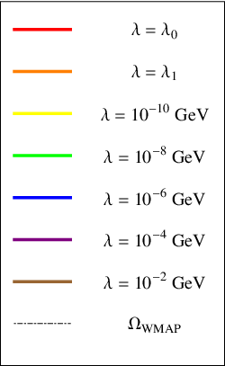


In order to illustrate the implications of these effects, in each of the panels of Figs. 4 and 4 we track the evolution of for a representative sample of within a given theory from to present time. The curves shown in Fig. 4 reflect typical results which arise in the context of the standard cosmology. The left panel corresponds to a scenario with a small confinement scale MeV, a moderate value GeV for the effective four-dimensional -breaking scale, and a small misalignment angle . The right panel corresponds to the opposite case: a scenario in which TeV, with GeV and . In each scenario, we have taken , and set the compactification scale to be GeV. The curves shown in each panel (from top to bottom) correspond to the lightest two values of , here referred to as and , corresponding to that particular choice of and ( GeV and GeV for the left panel; GeV and GeV for the right panel), along with several additional values of , including GeV. It should be noted that in the right panel, all curves shown lie essentially on top of one another, and are thus not individually apparent. It is worth remarking that in the scenario depicted in the left panel, while in the scenario depicted in the right panel. Also shown are a horizontal, dot-dashed line indicating the value for observed by the WMAP experiment [3], as quoted in Eq. (1), and a pair of vertical lines indicating the positions of and .
Both of these scenarios yield a total dark-matter relic abundance which is consistent with the WMAP results given in Eq. (1). However, it should be noted that the parameter assignments used for these figures have been chosen exclusively for purposes of illustration. In Sect. VI, we will discuss the situation using the parameters which are consistent with all observational and phenomenological constraints.
Note that the sets of curves shown in the two panels of Fig. 4 differ quite significantly. For example, in the left panel, the effect of the non-zero decay widths of the heavier is readily apparent. Indeed, the curves corresponding to masses GeV rapidly drop to zero at a time scale . By contrast, in the right plot, which corresponds to a scenario with , the decay rate of each is suppressed by a factor of , which can be quite small in such a scenario. Consequently, all of the for which curves are shown in the plot are stable on cosmological time scales.
The abundance curves shown in Fig. 4, on the other hand, display typical results obtained in the LTR cosmology. More specifically, the results shown here correspond to the parameter assignments MeV and GeV. As in Fig. 4, the two panels shown in this figure correspond to two different choices for , , and which both yield a total present-day relic abundance consistent with WMAP data. The curves shown in the left panel correspond to a scenario with GeV, GeV, and MeV. This scenario exemplifies the case in which and are both comparatively small. By contrast, the curves displayed in the right panel correspond to a scenario with far larger values for these parameters: GeV and TeV, with GeV. In both cases, we have taken . Once again, the curves shown in each plot correspond to GeV, as well as and . For the left plot, GeV and GeV; for the right plot, GeV and GeV. Again, in the left panel, the and curves are not apparent because they lie directly beneath the GeV curve.
The contrasting features between the two panels in Fig. 4 are predominately due to the differences between their and values. First, as stated above, is quite small in the scenario displayed in the left panel, and consequently, the couplings between the and the fields of the SM are quite large. This implies that the decay rates associated with the heavier will be sizable in this scenario, and that a large number of these heavier modes will decay before present time. Indeed, the precipitous drop in each of the curves corresponding to a mass eigenvalue in the range GeV in this plot is a consequence of the decay of these modes to SM fields. By contrast, in the scenario displayed in the right plot, is large enough that all of the for which curves are shown are stable on cosmological time scales, and no such effect is apparent. Second, is also quite small in the scenario displayed in the left panel, and the confinement time scale s is consequently quite late. As a result, for all . This implies not only that all of the modes begin oscillating at the same time, but moreover, that the only become non-zero quite late. By contrast, in the right panel, is large and is correspondingly quite early. This results in a situation in which the for the lighter modes are staggered in time. As discussed in Ref. [1], the primary consequence of this staggering is that the curves for these lighter modes depend more sensitively on .
The most important implication of Eqs. (62) through (65), however, is that decreases with increasing regardless of the details of the cosmological framework. On the other hand, we saw in Sect. III that increases monotonically with . This observation is indeed encouraging, in that it suggests that and possess the appropriate, reciprocal relationship needed for an ensemble of to serve as dynamical dark matter. In the following section, we will quantify more precisely the relationship between and and demonstrate that this is indeed the case. The results of the present section therefore attest that misalignment production, in stark contrast to thermal production, is an ideal mechanism for the generation of axion relic abundances in dynamical dark-matter models. Moreover, as we shall soon demonstrate, this mechanism dominates in the regime of model-parameter space in which an ensemble of tends to be phenomenologically viable, in the sense that it correctly reproduces the observed dark-matter relic abundance, while at the same time satisfying all relevant constraints from experiment, astrophysical observation, and cosmology.
Before we proceed to analyze the collective properties of such ensembles, however, two brief comments are in order. The first of these concerns the validity of the rapid-turn-on approximation. As we have stated above, Eq. (50) is strictly valid only when and are essentially independent of temperature. However, there turn out to be certain situations in which the time-dependence of and at temperatures is physically unimportant, and in which these quantities can be reliably treated as constants throughout the period in which are oscillating. One such situation arises in cases in which for all of the which contribute meaningfully to the total dark-matter relic abundance, and therefore coherent axion oscillations do not occur until after is effectively constant. This situation tends to arise either when is quite large, in which case attains its constant, late-time value very early, or else when is fairly small, but is quite large, in which case itself is extremely small. As we shall see in Sect. V, these turn out to be precisely the situations in which the total relic-abundance contribution from the ensemble of successfully reproduces the observed value for quoted in Eq. (1). This retroactively justifies our use of the rapid-turn-on approximation.
Our second comment concerns the assumption that is sufficiently small that the solution of Eq. (50) for any given includes a period during which this equation of motion is effectively underdamped. This is critical, since in the absence of such a period, coherent oscillations cannot occur. Indeed, the energy density stored in any for which would never scale in an appropriate manner for that field to behave like massive matter; hence it would never contribute to . However, it is not difficult to demonstrate that this situation essentially never arises in realistic bulk-axion scenarios, even for the most massive modes in a given tower. For example, consider the case of a purely photonic axion with . In this case, it follows from Eq. (31) that the solution for becomes critically damped at a value , which is determined by the condition
| (66) |
Solving this equation for , we find that
| (67) |
which implies that . However, since the effective description of the theory in terms of a tower of axion modes breaks down at the five-dimensional -breaking scale , we are assured that for all modes in such a tower. Indeed, this qualitative result is not specific to a photonic axion, but applies broadly to any axion field which couples to the SM fields with coupling coefficients. As a corollary, this result also implies that the standard oscillation criterion will always be met before the decay criterion . This indicates that indeed , rather than , sets the time scale at which oscillations begin, and that any given decays during a time frame in which its energy density can legitimately be described by Eq. (57).
V Characterizing the Ensemble: Total Abundances,
Tower
Fractions, and Equations of State
In the previous two sections, we derived expressions for the decay widths and relic abundances for the individual mass eigenstates in a mixed tower of KK axions. We have shown that these quantities scale with in an appropriate, reciprocal manner for an ensemble of such states to serve as dynamical dark matter. We are therefore finally equipped to address the dark-matter phenomenology of the ensemble as a whole.
As discussed in Ref. [1], the crucial quantities which characterize a given dynamical dark-matter ensemble are the total relic abundance , the tower fraction , and the effective equation-of-state parameter . In this section, we investigate how these three quantities depend on the scales , , and which characterize a given bulk-axion model and thereby assess which regions of parameter space are interesting from a dynamical dark-matter perspective. In the next section, we discuss the applicable phenomenological constraints on the model and demonstrate that substantial regions of parameter space exist within which all such constraints are satisfied.
V.1 General Definitions
The first of the three principal quantities mentioned above which characterize any given dynamical dark-matter ensemble is . This is simply the total contribution to from all constituent modes in the ensemble which have already begun oscillating:
| (68) |
The second is the so-called “tower fraction” , which is a measure of how the total abundance is distributed across the ensemble. Specifically, is defined for a given dynamical dark-matter ensemble to be the fraction of provided by all of the oscillating components of that ensemble except for the one which yields the largest individual contribution. Explicitly,
| (69) |
where . After all the have begun oscillating, the lightest mass eigenstate always yields the largest individual relic abundance , and therefore . When , essentially the entirety of is provided by a single field, as in most traditional dark-matter models. By contrast, having signals a departure from this traditional setup, which is indeed one of the hallmarks of dynamical dark matter. (Note that when we say that should differ significantly from zero, we are willing to accept , as such values could result in observable differences from traditional models, but not, for example, .)
In our dynamical dark-matter framework, both and are intrinsically dynamical quantities, with non-trivial time dependences. For this reason, we will designate their present-day values as and in what follows.
As discussed in Ref. [1], a given dynamical dark-matter ensemble as a whole can also be described in terms of a single, effective equation-of-state parameter :
| (70) |
where . Indeed, one of the hallmarks of this framework is that even itself is continually changing in time. We shall therefore define . As discussed in Ref. [1], this quantity is given by
| (71) |
for any given dynamical dark-matter ensemble in which the widths, abundances, and densities of states obey the approximate scaling relations and , where denotes the density of states per unit decay width.
Taken together, , , and serve to characterize any given dynamical dark-matter ensemble. For the remainder of this section, then, our task will be to investigate how these three quantities depend on the parameters , , and which characterize our bulk-axion model. Also recall that in Eq. (23) we defined the mixing parameter
| (72) |
which quantifies the extent to which the different modes in the KK tower mix with each other. We will also therefore keep track of the corresponding values of in our analysis. Moreover, as we have seen in Sect. IV, our results will also depend on the cosmological framework adopted. We shall therefore derive results in the context of the standard and LTR cosmologies independently. However, as discussed above, constraints on in theories with large, flat extra dimensions provide a strong motivation for working within the context of an LTR cosmology with a reheating temperature . For this reason, the results obtained for the LTR cosmology are more likely to be realistic.
Needless to say, phenomenological consistency imposes certain constraints on the parameters , , and . For example, WMAP data require that ; likewise, should not differ too significantly from zero. Beyond this, however, and are fairly unconstrained by data. Nevertheless, while any values for and can be realized within the general dynamical dark-matter framework, we are particularly interested in situations in which is also significantly different from zero, for these are the situations in which our dynamical dark-matter ensemble represents a significant departure from traditional, single-component models of dark matter.
V.2 Dark Towers: Relic Abundances and Tower Fractions
In Fig. 5, we show how the total present-day dark-matter relic abundance depends on , , and in the standard cosmology, assuming a photonic axion with . Each panel in the figure displays contours of for a different choice of . A dashed blue line highlighting the contour has also been included in each panel. The red lines are contours of : the solid red line corresponds to , which roughly indicates the transition point between the strongly-mixed regime (below and to the left of the contour) and the weakly-mixed regime (above and to the right of the contour). Proceeding from left to right, the dotted lines correspond to the values . In Fig. 6, we present the corresponding contour plots for the tower fraction . Moreover, to complement the results shown in Figs. 5 and 6 for the standard cosmology, we present the corresponding results for the LTR cosmology in Figs. 7 and 8.


As Figs. 5 and 7 illustrate, the dependence of on the model parameters , , and is somewhat complicated, and the results displayed therein clearly warrant detailed explanation. Perhaps the most intuitive way of understanding these results is to begin by examining them in certain limiting regimes. For example, consider a situation in which is relatively small. In this case, the confinement time scale is relatively late. If is sufficiently late that all modes in the tower begin oscillating immediately at , each is given in the standard cosmology by Eq. (62) for all and by Eq. (63) in the LTR cosmology. In addition, let us assume that is large enough that decays can be neglected, and that is at least moderately large, so that essentially all of the which contribute meaningfully to survive inflation. In this special case, we can explicitly sum the contributions to obtain the result
| (73) |
In deriving this result, we have used the second identity in Eq. (27). Note that Eq. (58) implies that ; hence is suppressed in the LTR cosmology relative to the standard cosmology by a factor which can be quite significant. Indeed, this suppression factor in is due to the uniform suppression of each individual contribution in this regime by the factor given for the case in Eq. (61).
Perhaps the most interesting aspect of this result is that it depends only on , and is independent of both and . This is quite surprising indeed, for it indicates that in this regime, no matter how many of the contribute significantly to , the total contribution to the dark-matter relic abundance is the same. For example, a strongly-mixed scenario with and a vast number of modes contribute more or less democratically to will yield the same abundance as a weakly-mixed scenario with in which a single, light axion accounts for essentially the entirety of the dark matter. This situation is realized in the MeV and MeV panels in Figs. 5 and 7, in which the value of remains essentially constant throughout the region of parameter space shown.
At an algebraic level, the fact that is a constant throughout substantial regions of space for small is a reflection of the fact that the identity in Eq. (27) holds regardless of the value of . Of course, this identity requires that the sum over be taken over the entire KK tower, from the lowest mass eigenstate up to infinity. At a physical level, this is the appropriate sum to take for small , because all of the modes begin oscillating at a common time , and because the full structure of the tower is undisturbed by the decay of any modes which contribute meaningfully in the sum. Indeed, as we have seen from the panels of Figs. 5 and 7, this result is characteristic of situations in which is small.
However, as we increase , three effects can begin to alter this picture and thereby destroy the uniformity of :
- •
First, becomes smaller and smaller, and consequently can begin to exceed for the lower modes in the KK tower. In other words, these lower modes may begin to experience oscillations with staggered onset times, a phenomenon which begins with the lowest-lying modes in the tower and ultimately affects higher and higher modes as increases.
- •
Second, decreases with increasing (for fixed and ), and consequently more and more of the excited contribute significantly to . Although the lifetimes of these modes also increase with increasing , they do so at a slower rate. As a result, a larger and larger fraction of the contributing portion of the KK tower is effectively truncated by decays. This effect can therefore lead to a reduction in , especially in the regime.
- •
Third, as increases, can be pushed back into the inflationary era. The contributions from those modes which begin oscillating prior to or during inflation will therefore be inflated away. This too can result in a reduction of .
Of course, which of these effects happens to be relevant in any given situation ultimately depends on the parameters in question, and whether we are working in the standard cosmology or an LTR cosmology. Let us therefore begin by examining the situation in the standard cosmology, as shown in Fig. 5. As we increase from MeV to TeV, we see that a series of contours with smaller and smaller values of emerges in the region of parameter space where and gradually spreads over a substantial region of space. This is the effect of decays truncating the contributions from the higher modes in the tower, as discussed above. Note that for the regions of parameter space shown in Fig. 5, neither of the other two effects outlined above is apparent. In particular, staggering effects only occur within regions of parameter space for which , where is the time at which the lightest mode in the tower begins oscillating. This criterion can be rephrased as a condition on the model parameters , , and by substituting for in the middle line of Eq. (46). In the and regimes, we can approximate and respectively to obtain
| (74) |
Given these results, it is clear that staggering effects will not be visible in Fig. 5: for the case, extremely large values of are required, regardless of the value of ; for the case, GeV or TeV is required for these effects to be apparent.
The situation is quite different in the LTR cosmology, as shown in Fig. 7. Indeed, as we increase , all three of the above effects begin to become relevant. First, we observe the same effect of decaying modes in the region that we saw in Fig. 5. This effect is particularly evident in the GeV panel of Fig. 7. However, in the LTR case, we also observe effects due to staggering, which begin to appear in the large- region. Indeed, following the same procedure applied above for the standard cosmology but using the top line in Eq. (46), we find that these effects emerge in regions of parameter space where
| (75) |
The first of these limiting forms accounts for the vertical contours which appear on the right side of the MeV panel in Fig. 7 and encroach further and further to the left as increases.
Finally, as grows beyond GeV, we see the third effect emerging: the inflating away of heavy KK modes. In particular, since we have chosen GeV in this plot, the relic-abundance contributions from all modes with will be inflated away. Indeed, we see that when (which implies that ) and GeV, the entire tower is inflated away, yielding . Indeed, since increases with for fixed and , this effect spreads across a wider region as increases.
Ultimately, for large , those modes which have not inflated away exhibit a completely staggered behavior in the LTR cosmology. This limit may be regarded as the converse of the “instantaneous turn-on” limit taken in Eq. (73) for small : indeed, we now have for all of the modes which contribute significantly to . Moreover, in this case the sum over can be explicitly evaluated using the first identity in Eq. (27), allowing us to obtain explicit results for in the completely staggered limit for both the standard and LTR cosmologies:
| (76) |
where for the standard-cosmology case. Note that the -dependence of is illustrated in Fig. 4 of Ref. [1]. In sharp contrast with the results obtained in Eq. (73), we see that in this staggered regime, the expressions for in the standard and LTR cosmologies differ significantly. In the standard cosmology, depends non-trivially on , , and (through its dependence on ). By contrast, in the LTR cosmology, depends on in this staggered-oscillation regime, but not on or .
Following similar reasoning, we can also understand the behavior of the tower fraction , beginning with the results displayed in Fig. 6 for the standard cosmology. These results nicely illustrate an important general property of in brane/bulk models of dynamical dark matter discussed in Ref. [1], which is that the behavior of is strongly correlated with the value of . In particular, when , the mass of the lightest mode in the KK tower is proportionally far lighter than those all of the excited modes, and consequently its contribution to the total abundance will be much larger than the contributions from all of those other modes combined. Indeed, this is nothing but the four-dimensional limit of the KK theory. This property of is independent of both the specific cosmological context and whether or not any of the modes in the tower have staggered oscillation onset times, as can be seen from Eqs. (62) through (65). By contrast, when , each mode with a mass contributes essentially equally toward when for all , and hence . This behavior is manifest in the various panels of Fig. 6, in which rapidly transitions from nearly zero to nearly unity as one crosses the contour.
In Fig. 8, we display the behavior of in the LTR cosmology. For small , the situation is very similar to that in the standard cosmology: all modes in the tower begin oscillating at , and hence for , while for . However, as increases, the oscillation onset times for more and more of the lighter modes in the tower become staggered in time. In this regime, the energy densities associated with the lighter modes in the tower scale like vacuum energy (and are hence unaffected by Hubble dilution) for a longer time before coherent oscillations set in and they begin to scale like massive matter, as illustrated in Fig. 1 of Ref. [1]. It follows that in this regime, the lighter modes account for a greater fraction of . For this reason, as discussed in Ref. [1], no longer approaches unity for in those regions of parameter space in which oscillation onset times are staggered, but instead asymptotes to11 1 Note that there are two (ultimately equivalent) ways to derive this result, corresponding to two different methods of taking the limit. In Ref. [1], we recognized that as . Since the limit also implies that for all , we can similarly approximate in this limit. We then have , whereupon it follows that , or equivalently . However, it is also possible to retain the exact form , whereupon we see that where is the value of for the lightest eigenvalue and where we have used the identity to perform the sum over KK modes. Note that this result is exact and valid for all . However, it is easy to verify that as . We thus again find that .
| (77) |
for the case of the LTR cosmology. Roughly speaking, the regions of parameter space in which this occurs are those in which the staggered-onset criteria in Eq. (75) are satisfied. Indeed, this effect first becomes apparent in the GeV panel of Fig. 8 and becomes increasingly significant as increases and staggering effects become relevant for smaller and smaller and larger and larger . By GeV, these staggering effects are realized over nearly the entirety of space shown, leaving only a narrow strip in which all modes still begin oscillating at , and by GeV, even this strip vanishes. Note also that the effect on of modes being inflated away is apparent in the upper left of those panels in Fig. 8 for which GeV. While is technically undefined in this region of parameter space because , we have set within this region to illustrate where this effect is relevant.
As discussed in the beginning of this section, the interesting regions of parameter space for dynamical dark matter are ultimately those in which , while at the same time differs significantly from zero. Given the results in Figs. 5 through 8, we can now determine whether this situation ever actually arises in our model. Comparing the results in Figs. 5 and 6, we see that this occurs in the standard cosmology for small values of , within a diagonal stripe of parameter space slightly to the left of the blue contour in each panel. We also see that this stripe moves to the right in space as increases. By contrast, comparing the results in Figs. 7 and 8, we see that the above conditions are satisfied in the LTR cosmology in the region of parameter space where
| (78) |
This result is certainly intriguing, as it suggests that the preferred scale for in this model is roughly the TeV scale for the LTR cosmology — a scale at which there is good reason to expect new physics to appear.
The principal message of Figs. 5 through 8, then, is that our bulk-axion model indeed satisfies the conditions on and for dynamical dark matter within these regions of parameter space. In other words, within these regions, our axion ensemble reproduces the observed dark-matter relic abundance, and does so in a non-trivial manner, with a substantial number of its constituents contributing significantly to . Of course these alone are not sufficient conditions for a successful model of dynamical dark matter: such a model must also not only have an appropriate present-day equation-of-state parameter , but also satisfy all additional relevant phenomenological constraints. In the remainder of this section, we will address the constraints on ; the rest of the applicable constraints will be addressed in Sect. VI.
One particular ramification of these constraints, however, is appropriate to mention before proceeding further. As discussed in Sect. IV, certain bounds which apply generically to models with large, flat extra dimensions strongly prefer the LTR cosmology over the standard cosmology. For this reason, we will focus primarily on the LTR case from this point forward.
V.3 Dark Towers: Equations of State
Having characterized the behavior of and over the parameter space of our bulk-axion model, we now proceed to discuss the third critical quantity which characterizes the dynamical dark-matter ensemble in this model: the present-day effective equation-of-state parameter . Since it is now clear which regions of model parameter space are suitable for dynamical dark matter, we will not perform a general survey of over the entirety of that parameter space, as we did with and , but instead focus on the preferred regions indicated in Eq. (78).
In order to calculate we need to know the values of the coefficients and exponents , , , and appearing in Eq. (71). This, in turn, requires knowledge of how our abundances and decay widths scale with . As in the previous subsection, we will assume that the abundances of the result from misalignment production, and likewise we will assume that their decay widths are those appropriate for a photonic axion with . Because the preferred region of parameter space specified in Eq. (78) for our model is one which is well approximated by assuming staggered oscillation onset times for all relevant modes, the correct expression for is the one given in Eq. (65). Likewise, the decay width for a photonic axion is given by the expression in Eq. (31). We therefore find that the coefficients and appearing in Eq. (71) are given respectively by
| (79) |
and
| (80) |
while the power-law indices and are given by
| (81) |
Substituting these results into Eq. (71), we find that
| (82) |
Let us discuss the implications of these results. First, it was noted in Ref. [1] that the effective equation-of-state parameter for any given dynamical dark-matter ensemble at any time will always fall within the range as long as . This makes such ensembles less dangerous from a phenomenological point of view. Indeed, we see from the results above that this criterion is satisfied for both the large- and small- regimes in the bulk-axion model under consideration here.
Second, in order to convey a sense of the characteristic size of in the favored region of parameter space for dynamical dark matter given in Eq. (78), we note that for the choice of GeV, GeV, and TeV, with , we find that for , while for . As these numbers are both extremely close to zero, we conclude that at present time our axion ensemble has an effective equation of state which can be legitimately interpreted as that of dark matter. Thus our ensemble meets all three requirements for a self-consistent model of dynamical dark matter.
VI Characterizing the Ensemble: Constraints and Prospects for Detection
In the previous section, we demonstrated that an ensemble of mixed KK excitations of a bulk axion field can collectively account for the observed relic abundance of dark matter in our universe. However, as discussed in Ref. [1], in order to be a viable model of dynamical dark matter, the model must also comply with a variety of additional laboratory, astrophysical, and cosmological constraints. Some of these constraints are intrinsic to any theory involving large extra dimensions, while others arise due to the physical effects of the axion field which propagates in the bulk of those dimensions. A number of analyses of such constraints exist in the literature [41, 26, 42] for the specific case in which the bulk axion in question is identified with the QCD axion and the fundamental, -dimensional quantum-gravity scale is taken to be roughly . By contrast, in the present analysis, we are interested in a broader class of axions which are neither required to couple to the fields of the SM (and in particular to hadrons) in the same manner as a QCD axion, nor subject to the same strict relationship between the suppression scale for those couplings and the axion mass. Moreover, our primary motivation is not to address the hierarchy problem, but to address the issue of what constitutes the non-baryonic dark matter in our universe. For these reasons, we will not focus exclusively on scenarios in which is at or near the TeV scale, but also consider scenarios with much larger . As a consequence, exclusion limits on the parameter space of the more general axion scenarios considered here can differ quite significantly from those presented in previous studies, and thus warrant reexamination.
We begin our summary of the applicable constraints on our model with a brief synopsis of those limits which arise generically in theories with large, flat extra dimensions and which do not depend on the presence or properties of the bulk axion field. For the most part, these limits, an overview of which was presented in Ref. [28], tend to derive from the non-observation of physical effects related to the dynamics of KK gravitons. These limits take many forms. First, there is the direct lower bound on quoted in Eq. (34) from experimental limits on modifications of Newton’s law at short distances due to KK-graviton exchange [32]. In addition, a number of constraints arise as a consequence of the production of these particles in the early universe [28, 36]. As discussed in Sect. IV, these cosmological constraints can collectively be addressed by positing that the universe underwent a late period of cosmic inflation with a reheating temperature . Thus, by adopting an LTR cosmology with a reheating temperature of this order, as we have done, we automatically ensure that a large number of these model-independent constraints are satisfied.
A number of additional constraints on theories of this sort can be derived from observational limits on KK-graviton production in astrophysical sources, such as stars [43] and supernovae [44, 45]. The most stringent of these constraints are currently those resulting from gravitationally trapped KK gravitons in the halos of neutron stars either decaying to photons or serving as a heat source for the stars themselves. In the case of flat extra dimensions with equal radii compactified on an -torus, these limits supersede the limit on given in Eq. (34). In particular, for , the bound is GeV, while for , one finds GeV [43]. However, if the radii of the extra dimensions differ from one another, or if the compactification manifold is not toroidal, these bounds can be considerably weaker. Furthermore, it is possible that the axion propagates only within some number of the additional dimensions, . In other words, the axion could be confined to a -dimensional brane within the bulk. In this case, the effective, four-dimensional scales and are related to the fundamental, higher-dimensional scales and in completely different ways:
| (83) |
The upshot, then, is that naïve limits on derived from KK-graviton dynamics under the assumption of toroidal compactification and equal radii do not necessarily translate in a straightforward manner into constraints on the mass scales relevant to the physics of a bulk axion. Fortunately, the bound in Eq. (34) is universal and is not sensitive to the total number of extra dimensions, unless they are each of comparable size. We will therefore take this bound to be the lower limit on in the model under consideration here.
We now turn to address those constraints which relate to the effects of the bulk axion itself. Indeed, a number of considerations serve to constrain the properties of light exotic particles with suppressed couplings to SM fields. Some of these constraints derive from observational limits on the production of such particles in astrophysical sources such as stars and supernovae; others derive from limits on the decays of a cosmological population of such fields into SM fields; and still others owe to direct experimental bounds from microwave-cavity experiments, helioscopes, etc. A detailed analysis of the exclusion limits implied by these constraints on general bulk-axion scenarios will be presented in Ref. [35]. Here, we merely summarize the results and discuss their implications for a mixed KK tower of axions as a model of dynamical dark matter.
As we shall discuss further in Ref. [35], it is convenient to separate the applicable constraints into four rough classes, based on the origin of the constraint and on the dynamics being probed. The first class of constraints which apply to scenarios of this sort are those related to the total present-day dark-matter relic abundance . Most of these bounds have been addressed in previous sections, but it will be useful to recapitulate them here:
- •
The axion ensemble must yield an acceptable contribution to the present-day dark-matter relic density. While is permitted, provided some additional field or fields make up the deficit, values of in excess of the WMAP upper bound in Eq. (1) are excluded.
- •
At no time in the past may our ensemble overclose or prematurely matter-dominate the universe.
- •
The present-day effective equation-of-state parameter for the ensemble must not deviate significantly from zero.
- •
Misalignment production must provide the dominant contribution to for all , and the population of hot axions generated via thermal production must be negligible. We therefore require that at all times after the end of cosmic inflation, where is the total production rate of axions from interactions with SM fields in the thermal bath.
- •
We have also assumed that the population of axions generated from the decays of cosmic strings associated with the breaking of the global symmetry is small compared to the population generated by misalignment production. We therefore impose the requirement that , so that such strings are diluted away by inflation.
- •
Our model must respect current observational limits on isocurvature fluctuations from WMAP [3].
The last of these constraints warrants additional discussion. Non-adiabatic fluctuations — also known as isocurvature fluctuations — refer to fluctuations not in the total energy density (which relates directly to spacetime curvature) but rather in how that total energy density is distributed among different contributing fields (including the collective contribution from the dark sector). Such isocurvature fluctuations are tightly constrained by a combination of CMB observations, baryon-acoustic-oscillation (BAO) measurements, and supernova data [3]. Such fluctuations generically arise whenever a cosmological population of particles is produced in a manner such that its primordial density perturbations are uncorrelated with those of the inflaton field. Indeed, limits on isocurvature fluctuations place severe constraints on the relic abundance of a standard QCD axion produced via vacuum misalignment [18], so it might reasonably be assumed that such limits might play a significant role in constraining our model as well.
It turns out, however, that our model satisfies the WMAP constraints on non-adiabatic fluctuations far more easily than do standard axion dark-matter models. A detailed discussion of these constraints and how they apply to bulk-axion models of dynamical dark-matter will be presented in Ref. [35], but the gist of the argument is as follows. Although our dynamical dark-matter ensemble comprises a large number of individual components , the fact that implies that the individual abundance associated with each of these components is actually quite small. Furthermore, the underlying five-dimensional nature of our KK axion tower guarantees that the primordial density fluctuations for each are all determined by the fluctuations of the same initial misalignment angle . For these reasons, the expected magnitude for isocurvature fluctuations in our model turns out to be no greater than it is in models in which misalignment production causes a single four-dimensional field to carry the complete dark-matter abundance. Moreover, if one assumes a Gaussian distribution for , it is straightforward to demonstrate [35] that . Thus, all that is required is that within our preferred regions of parameter space. However, as discussed in Eq. (78), the phenomenologically preferred scale for in our model is roughly . For at or around this scale, it turns out that current constraints on isocurvature fluctuations can be satisfied, provided that GeV. Such a scale for is easy to realize in traditional cosmological scenarios, and is even more natural in LTR cosmologies wherein the reheating temperature is . Thus, in our model, it is not difficult to satisfy current isocurvature bounds while simultaneously obtaining a total relic abundance .
The underlying reason why our model easily evades these non-adiabatic constraints is that within the preferred region of parameter space in Eq. (78), the five-dimensional axion in our model is not the standard QCD axion. In particular, we see that the scale is significantly larger than . Our model is thus freed from the implicit parametric dependence on which afflicts more traditional models of axion dark matter, and allows the corresponding non-adiabatic fluctuations to have a much smaller scale.
A second class of constraints comprises those observational limits on processes in which axions are produced via their interactions with the fields of the SM and then subsequently detected via those same interactions. These include:
- •
Limits from helioscope experiments, such as CAST [46], which search for axions produced by interactions with SM particles in the sun via their “conversion” to photons in the presence of a magnetic field.
- •
Limits from light-shining-through-walls (LSW) experiments (see Ref. [47] for a thorough review), including those by the BEV and GammaeV collaborations.
The most stringent of these bounds is currently that from CAST; we shall therefore take the CAST bound as representative of this class.
The physical processes to which this second class of limits applies are all subject to a particular effect which arises universally in models with both brane and bulk mass terms. This is the phenomenon of decoherence discussed in Refs. [26, 1]. This decoherence phenomenon can substantially suppress the cross-sections for such processes in our model, and thereby significantly weaken the bounds on , , and . To summarize, the cross-section for any process in which axions are produced at some time and then subsequently detected at a later time is given by
| (84) |
where is the number of modes contributing in the sum and where is the detection probability at time . This latter quantity is given in the relativistic limit by [26]
| (85) |
where is the initial momentum of the axion. For any reasonable choice of model parameters, the sum in the second term decoheres on time scale so rapid as to be effectively instantaneous [26]. As a result, is suppressed, relative to the naïve expectation, by an additional factor of . This effect considerably weakens the constraints in this class.
A third class of constraints can be derived from processes in which axions are produced via their interactions with SM fields but not subsequently detected. Instead, the presence of the axions is made manifest by their ability to carry away momentum and energy from a given system. These constraints include:
- •
Observational limits on the energy loss in supernovae, and, in particular, on the fraction of the energy released by SN1987A in the form of light exotic fields [48].
- •
Limits related to the effects of energy dissipation by axions on stellar lifetimes. The most stringent such limits currently come from observations of globular-cluster stars [32], but similar limits have also been derived from constraints on the lifetimes or energy-loss rates of other astrophysical bodies (e.g., the sun [49] and white dwarfs [50]).
- •
Constraints from the absence of observed signals in channels such as and at particle colliders. In general, the constraints on axion production in these channels are analogous to the well-known constraints on KK-graviton production [52].
- •
Limits on the branching fractions in particular exotic decay channels for certain hadrons [51].
The degree to which many of these limits constrain the parameter space of bulk-axion scenarios depends quite crucially on how the axion in question couples to the fields of the SM. Moreover, many of the constraints in this class are considerably relaxed in regions of parameter space in which , due to the coupling-suppression phenomenon discussed in Ref. [1]. This effect will be discussed in greater detail in Ref. [35].
A fourth and final class of constraints is related to the interactions and decays of a cosmological population of axions. Depending on the cosmological epoch during which such decays occur, they can result in a number of potential signals, none of which have been observed to date. For example, these include:
- •
Decays of cosmic axions which occur after the beginning of the BBN epoch (at around s), but before last scattering (at around s). These could disrupt nucleosynthesis and affect the abundances of light elements [53].
- •
Photoproduction (either primary or secondary) from any axion decays that occur between the epoch of electron-positron annihilation (at around s) and last scattering. These can lead to observable distortions of the CMB [54].
- •
Photoproduction (either primary or secondary) from any axion decays that occur after last scattering. These can lead to peaks and other indicative features in the diffuse X-ray and gamma-ray spectra [55], but such features have not been observed by FERMI [56], EGRET [57], COMPTEL [58, 59], or any other X-ray or gamma-ray telescope [60, 62, 61].
- •
Entropy production from late axion decays. This can have observational effects on cosmological parameters, such as the rate of cosmic expansion.
- •
It should be reiterated that the vast majority of the constraints enumerated above are highly model-dependent. The standard energy-dissipation limit from SN1987A [48], for example, provides one of the most stringent limits on the parameter space of a QCD axion. However, these limits are predicated on the assumption that the axion couples to hadrons with significant strength, and that processes such as consequently dominate the axion-production rate. A purely photonic axion, on the other hand, lacks such couplings, and hence can only be generated via interactions such as the Primakoff process , for which the rate is much smaller. As a result, the bounds on , , and for such an axion are considerably weaker than those for a hadronic axion (see, for example, Refs. [65, 51] for an analysis of this constraint for a four-dimensional photonic axion). A variety of other constraints, including bounds from monojet searches at hadron colliders and from the requirement that misalignment production of axions dominates over thermal production, also differ markedly depending on whether or not the axion in question couples to hadrons. Still other bounds, such as that from energy loss in white dwarfs [50], depend sensitively on whether or not a given axion couples to leptons.


In Figs. 10 and 10, we display a series of exclusion plots in space, taken from Ref. [35], which indicate the regions of parameter space excluded by the considerations enumerated above. The three panels in Fig. 10 correspond to for the case of a photonic axion with , while the three panels in Fig. 10 correspond to the same choices of , but for a hadronic axion with . In each case, we have taken , with MeV and GeV; for the hadronic case, we have also assumed that , , etc., take the values given in Eqs. (9) and (10). The shaded regions in each panel are excluded by the battery of constraints discussed above. The red region is excluded by CAST data, the magenta region by limits on collider processes in which axions appear as missing energy, the purple region by limits on modifications of Newton’s law from Eötvös-type experiments, the orange region by limits on distinguishable features in the diffuse extragalactic X-ray and gamma-ray background spectra, the yellow region by observations of the lifetimes of globular-cluster stars, the cyan region by energy-loss limits from supernova SN1987A, the gray region by the model-consistency requirement that , and the brown region by the upper bound on the dark-matter relic abundance from WMAP. A black, dashed line corresponding to the condition has also been included in each panel for reference. Note that each of the exclusion regions shown, with the exception of that from WMAP, differs from the corresponding exclusion region for a four-dimensional axion. The exclusion regions shown are those appropriate for the five-dimensional axion on which our model is based, and are derived in Ref. [35].
The constraints enumerated above for which no exclusion contour has been included in these figures are generally subleading. For example, the applicable constraints from exotic hadron decays [51] are generally far weaker than the constraints from SN1987A, thermal production, etc., for any given choice of parameters. The constraints arising from observational limits on distortions of the CMB are not particularly stringent either, and turn out not to constrain any portion of the model parameter space shown in any of the panels appearing in Figs. 10 and 10. This is because the regions of parameter space in which the are sizeable are those in which is quite small, meaning that the are also quite small, as is evident from Fig. 7. Constraints related to the effects of late-decaying on BBN were not explicitly calculated in Ref. [35]. However, exclusion contours derived from BBN constraints on late-decaying particles are expected to be roughly similar to those derived from CMB constraints, and consequently such constraints are not expected to rule out any additional region of model parameter space not already excluded by other considerations. Limits on the effective equation-of-state parameter are not particularly constraining either. This should come as no surprise, given that we showed in Sect. V that the effect of decays on was negligible within the region of parameter space relevant for dynamical dark matter. A number of additional constraints not listed above also serve to constrain very light axions and axion-like particles [66]; however the particles for which these constraints apply typically involve values of far smaller than those of interest here.
It is evident from these figures that the most stringent constraints on both photonic and hadronic axions are those from SN1987A (cyan) and from collider limits on missing-energy processes (magenta). Nevertheless, it is also evident that a hadronic axion is significantly more constrained than a purely photonic axion. As discussed above, the primary reason for this is that the rate of axion production in a thermal setting via interactions with nuclei, pions, etc., is far larger than the corresponding rate of production via the electron Primakoff process and other interactions which involve the coupling of an axion to photons alone.
Having assessed the phenomenological constraints on a bulk axion, we are now able to definitively address the question as to whether or not our model is a viable model of dynamical dark-matter. In order for this to be so, we require that at least some part of the preferred region in Eq. (78) be consistent with the constraints discussed above. Inspecting Figs. 10 and 10, we see that indeed our preferred region is compatible with all of these constraints in both the photonic and hadronic axion cases for GeV, with above the lower bound from Newton’s-law modification, but small enough so that . Furthermore, we also see from Figs. 10 and 10 that the phenomenological constraints even permit us to reach deeply into the region. Note that this represents a radical departure from the QCD-axion results presented in Ref. [26] — a departure which is enabled because is a free parameter in our model. Thus, we conclude that within this region of parameter space, our bulk-axion model constitutes a viable, explicit model of dynamical dark matter.
It should be stated that in addition to the limits discussed above, certain additional astrophysical bounds may also serve to constrain the parameter space of bulk-axion scenarios. For example, it has recently been shown [67] that limits on gamma-ray signals from decaying axions with masses of produced in supernovae can yield an even more stringent limit than that arising from energy-dissipation considerations alone. While these bounds are once again model-dependent (and directly applicable only to cases in which the axion in question couples directly to hadrons with significant strength, and not to a photonic axion), they could provide an important additional constraint on the parameter space of dynamical dark-matter scenarios involving bulk axions. Furthermore, it is also possible that comparable bounds could be obtained from an analysis of photo-emission limits and cooling-rate constraints from neutron stars, similar to that performed for KK gravitons in Ref. [43].
It is important to note that while additional bounds related to axion production in supernovae may serve to further constrain the parameter space of bulk-axion scenarios, these constraints cannot rule out axion models of dynamical dark matter entirely. This is due to the fact that for any given choice of model parameters , , and , the couplings of any mode for which to the SM fields will be suppressed by mixing effects, as discussed in Ref. [1]. Indeed, because we can reach deeply into the region, the magnitude of this coupling suppression can be quite significant. For example, for , we find that the first twenty axion mass eigenmodes have coupling suppressions . If the coupling suppressions are significant for those with masses in the “dangerous” range MeV discussed above, such will be produced in supernovae at a negligible rate, and thus all supernova bounds on axion production can be evaded. This can be arranged by demanding that GeV, so that all modes with masses GeV are effectively in the small- regime. Therefore, since is essentially independent of within our preferred region of parameter space, satisfying this condition is simply a matter of choosing a sufficiently large value for . Indeed, setting GeV in accord with Eq. (78), we find that all axion-production constraints from supernovae can be avoided for
| (86) |
We emphasize that this rough bound is not a necessary condition for consistency with supernova data, but a sufficient one. Furthermore, since the neutron-star cooling and photo-emission bounds on KK gravitons rest on the assumption that a population of gravitationally-bound particles of this sort was generated by the supernova whose core-collapse produced a given neutron star, any similar bound on axions would also cease to apply in this regime. We also note that since the fundamental scale is still roughly an order of magnitude larger than the value of required to satisfy this condition, given the input values of and , no theoretical inconsistency results from positing a confinement scale of this order.
The fact that this coupling-suppression phenomenon is capable of rendering our model consistent with supernova bounds despite the large multiplicity of light modes attests to the importance of this effect in brane/bulk theories. A more detailed overview of this phenomenon and its physical implications will be provided in Ref. [35].
VII Discussion and Conclusions
The aim of this paper has been to present an explicit realization of the dynamical dark-matter framework presented in Ref. [1]. To that end, we have shown that an ensemble consisting of the KK excitations of a light, axion-like field can indeed provide such a realization. Indeed, we have shown that despite the fact that the masses, decay widths, and relic abundances of all of these particles are controlled by only three dimensionful parameters, the ensemble to which they give rise is simultaneously able to reproduce the observed value of and satisfy all applicable constraints from laboratory experiments, astrophysics, and cosmology. As such, this model provides a “proof of concept” for dynamical dark matter as a viable alternative framework for dark-matter physics. In addition, it also provides a method of addressing the dark-matter question which does not require the introduction of any additional stabilizing symmetry.
Many qualifications, extensions, and possible generalizations of our dynamical dark-matter framework were discussed at the end of Ref. [1]; here, we shall restrict our attention to five points which are specific to the bulk-axion model presented in this paper.
- •
First, in this work, we have made use of the rapid-turn-on approximation in Eq. (52) in calculating the relic abundances of the . As discussed in Sect. IV, this approximation is well motivated, since the instanton-generated mass term falls rapidly with temperature when . Furthermore, the primary results of this paper are essentially insensitive to this approximation. This is because the fields which contribute significantly to in regions of parameter space which yield a realistic dark-matter relic abundance begin oscillating only well after has already settled into its constant, late-time value. However, the relic abundance of any field which begins oscillating before takes this late-time value will, in general, depend on the details of how this mass evolves in time. The quantitative effect on the abundance of a single field has long been appreciated [22], but in our model, the effects are more complicated and more subtle because we have a coupled system of mixed scalars with different masses and therefore different oscillation times. It would be interesting to examine how a more rigorous treatment of the turn-on of would affect and in situations in which these quantities are sensitive to the time-dependence of this brane-mass term. Such a study would have important implications for more general scenarios involving other kinds of light bulk scalars. Indeed, the relationship between the size of the brane-mass term for such scalars and the time at which that brane mass is dynamically generated may differ significantly from the relationship which holds for axions.
- •
Second, as alluded to in Sect. VI, it may be possible to further test or constrain the parameter space of bulk-axion models of dynamical dark matter in a number of ways. We have already mentioned one potential constraint which derives from limits on high-energy photons resulting from the decays of axions produced in supernovae [67]. Other considerations also merit investigation. For example, a detailed analysis of the limits imposed by BBN on scenarios involving multiple decaying fields with different lifetimes and abundances could provide important constraints on dynamical dark-matter models in general. In addition, other considerations, such as limits on mass loss and decreases in the dark-matter density in the halos of dwarf galaxies [68], could also be used to constrain dynamical dark-matter models. Indeed, while a number of standard constraints on individual unstable relic particles in the early universe have been revisited in a dynamical dark-matter context [35], it would be interesting to see how other constraints would apply in this context as well.
- •
Third, we note that we have not specified a particular model of inflation as part of the cosmological context for our model. Indeed, other than requiring a low reheating temperature , we have remained largely agnostic about the details of the inflationary model, the form of the inflaton potential, or even the scale . For the most part, our model does not depend on these particulars. However, certain consistency conditions do place meaningful restrictions on the set of inflationary scenarios with which our model is compatible. One such condition can be derived from the fact that vacuum fluctuations during inflation generically give rise to a background value for any scalar with a mass , where is the duration of inflation. This implies that the relationship between the mass and initial energy density in Eq. (56) in our model is truly valid only for the lighter in a given tower — i.e., those for which . By contrast, any heavier which still satisfy receive the leading contributions to their background values from vacuum fluctuations during inflation, and thus effectively acquire an initial abundance . In typical scenarios, we expect , where is the number of -foldings of inflation. The results for derived in Sect. V therefore remain consistent, provided that . Indeed, since GeV within the preferred region of parameter space specified in Eq. (78), we see that is certainly not inconsistent with our model and is in fact even expected. However, this condition on has non-trivial implications for inflationary models. While a low scale for is certainly not excluded (see, e.g., Refs. [39, 69]), extremely small values of tend to be rather non-generic [70] among typical classes of inflationary potentials, and thus require either substantial tuning or careful construction. Indeed, any consistent inflationary model of this sort must give rise to density fluctuations on a scale consistent with constraints from CMB data [3], such as those on the spectral index , and must also satisfy other observational constraints. The development of explicit inflationary scenarios of this sort is therefore an interesting topic for future investigation.
- •
Fourth, we note that while we have chosen in this paper to focus on the case in which the ensemble of fields reproducing are the KK excitations of a bulk axion field, such a field is by no means unique in possessing the characteristics necessary to give rise to such an ensemble. Indeed, as discussed in Ref. [1], much of the analysis presented here pertains to any light bulk scalar for which a mass term is dynamically generated via its interactions with brane-localized fields. Furthermore, for a generic bulk scalar, the relationship between the time at which this mass term is dynamically generated and the magnitude of this mass term itself may differ from that which relates and for a bulk axion. As a result, much more freedom may exist for constructing viable models within the dynamical dark-matter framework. For example, light moduli could also, in principle, provide a viable model of dynamical dark matter.
- •
Finally, we emphasize that the presence of additional axion-like fields is fairly generic, and perhaps even expected, in many theoretically motivated scenarios for physics beyond the Standard Model (see, e.g., Ref. [25]). Moreover, it has even been argued that many of these axion-like fields are likely to be light [66]. Thus, the discovery of a vast ensemble of axion-like particles could provide important insight into what physics looks like at high scales. Indeed, if many of these axions have relatively small masses, we find ourselves in the intriguing situation in which most of the matter in the universe is simultaneously both light and dark.
Our goal in this work has been to provide an existence proof for dynamical dark matter — i.e., to provide a model in which lifetimes are balanced against abundances in such a way that the ensemble of dark-matter particles successfully reproduces while at the same time satisfying all phenomenological constraints. As we have seen in this paper, our bulk-axion model indeed passes this test. In one sense, our model does so in the most interesting way possible: with (signifying that our tower of axion KK modes is highly mixed) and with a tower fraction which is significantly different from zero. In another sense, however, this model is fairly conservative: those modes which contribute most to turn out to be rather long-lived, and likewise our numerical result for within the preferred region of parameter space turns out to be rather close to zero. Indeed, at first glance, one might suspect that these latter properties are in fact generic for dynamical dark-matter models, or even that such models are therefore really no different from traditional dark-matter models in terms of their abundance and stability requirements.
This is not the case, however, for the balancing of lifetimes against abundances — which is the hallmark of the dynamical dark-matter framework — is precisely why this framework does not require such a degree of stability, much less the existence of a stabilizing symmetry. While certain accidental features of our bulk-axion model result in a preferred region of parameter space which is somewhat conservative, we emphasize that these features are not generic even to theories with bulk scalars, much less realistic dynamical dark-matter models as a whole. Note, for example, that a particular relationship exists in bulk-axion models between the mass of a given KK mass eigenstate , the strength of its effective coupling to SM fields, and the overall magnitude of its relic abundance through the dependence of these quantities on . Even for other bulk scalars (e.g., moduli), these relationships do not necessarily hold. There is therefore no reason to expect dynamical dark-matter models based around such fields to be as conservative as the axion model we have presented here.
In this connection, there is an even more important point that deserves emphasis. In dynamical dark-matter scenarios, we have no single characteristic decay width nor abundance , but rather an entire spectrum of widths and abundances . This therefore begs the fundamental question: if our “proof of concept” model presented here is to be viewed as somewhat conservative, how far from the conservative limit can we go?
At first glance, one might try to answer this question by attempting to determine, for each time during the evolution of the universe, the maximum abundance that a given component in a dark-matter ensemble may have if it has a lifetime . In other words, given the entirety of the cosmological constraints from BBN, CMB distortions, etc., there exists a function which describes the maximum abundance any dark-matter constituent may have as a function of its decay width. It might therefore seem that knowledge of this function would uniquely determine the full range of possibilities inherent in our dynamical dark-matter framework.
Such an approach to answering our fundamental question is, in a sense, already a departure from the usual manner of approaching dark-matter physics. However, even the notion of such a function relies too strongly on a single-particle perspective. One of the critical features of our dynamical dark-matter framework is that it involves a vast ensemble of dark-matter components. Some of these components might decay earlier in cosmological evolution, while others might decay later. As a result, the maximum abundance that a given component may have if it decays on a characteristic time scale will itself be directly affected not only by the abundances of all of the other components with earlier characteristic decay times , but even the components with . Moreover, as we have seen, most phenomenological constraints on dark-matter decays are sensitive not merely to what happens at a specific moment in time, but to the integrated effects of such decays over a broad range of time scales. In other words, our dynamical dark-matter framework teaches us that astrophysical and cosmological constraints do not lead to a single function , but rather a more subtle set of intertwined constraints on lifetimes and abundances across our entire dark-matter ensemble as a whole.
Clearly, this issue has not been studied in any detail in the literature. However, it is readily apparent that this is indeed the only proper way in which one should express constraints on particle decays from a generic dark sector. Viewed from this perspective, then, the existence of even one viable dynamical dark-matter model — no matter how “conservative” it might be — gives us strong motivation to re-examine cosmological and astrophysical constraints within this framework. Indeed, it is only in this way that we will be able to fully explore our dynamical dark-matter framework, and understand its full range of phenomenological possibilities.
Acknowledgements.
We would like to thank K. Abazajian, Z. Chacko, D. Chung, M. Drees, J. Feng, J. Kost, J. Kumar, R. Mohapatra, S. Su, T. Tait, X. Tata, and N. Weiner for discussions. This work was supported in part by the Department of Energy under Grants DE-FG02-04ER41291 and DE-FG02-04ER-41298. The opinions and conclusions expressed here are those of the authors, and do not represent either the Department of Energy or the National Science Foundation.Appendix A Evolution of a Decaying Axion Field
For completeness, in this Appendix we provide exact solutions to Eq. (50) for a real-valued function . These take the form
| (87) |
where and are undetermined constants, and
| (88) |
In these expressions, , was defined in Eq. (51), denotes Kummer’s confluent hypergeometric function
| (89) |
where is the Pochhammer function, and denotes the Tricomi confluent hypergeometric function
| (90) |
It can be verified upon setting that Eq. (87) reduces to the exact form obtained for a tower of stable KK axions in Ref. [26].
The values of and in Eq. (87) are determined by the initial conditions chosen for and at , where is some initial time. Expressed in terms of these initial values, this equation takes the general form
| (91) |
where the time derivatives of and have the explicit forms
| (92) | |||||
Once again, if we set in this expression (which also implies that ), we recover the result
| (93) |
which agrees with the result obtained in Ref. [26].
In the rapid-turn-on approximation, in which takes the Heaviside form specified in Eq. (52), the initial conditions for and at take the form given in Eq. (53). Upon substituting these initial conditions into Eq. (91), we find that during the cosmological epoch in which coherent oscillations of a given begin, we have
| (94) |
The value of any during subsequent epochs can then be obtained iteratively from this relation.
References
- [1] K. R. Dienes and B. Thomas, “Dynamical Dark Matter: I. Theoretical Overview,” arXiv:1106.4546 [hep-ph] (to appear in Phys. Rev. D).
- [2]
G. Jungman, M. Kamionkowski and K. Griest,
Phys. Rept. 267, 195 (1996)
[arXiv:hep-ph/9506380];
K. A. Olive, [arXiv:astro-ph/0301505];
D. Hooper, [arXiv:0901.4090 [hep-ph]];
N. Weiner, “Dark Matter Theory,” video lectures given at TASI 2009,
http://physicslearning2.colorado.edu/tasi/tasi_2009/tasi_2009.htm;
J. L. Feng, Ann. Rev. Astron. Astrophys. 48, 495 (2010) [arXiv:1003.0904 [astro-ph.CO]]. - [3] E. Komatsu et al. [WMAP Collaboration], Astrophys. J. Suppl. 180, 330 (2009) [arXiv:0803.0547 [astro-ph]].
- [4]
X. L. Chen and M. Kamionkowski,
Phys. Rev. D 70, 043502 (2004)
[arXiv:astro-ph/0310473];
L. Zhang, X. Chen, M. Kamionkowski, Z. G. Si and Z. Zheng, Phys. Rev. D 76, 061301 (2007) [arXiv:0704.2444 [astro-ph]]. - [5]
C. Boehm, P. Fayet and J. Silk,
Phys. Rev. D 69, 101302 (2004)
[arXiv:hep-ph/0311143];
E. Ma, Annales Fond. Broglie 31, 285 (2006) [arXiv:hep-ph/0607142];
T. Hur, H. S. Lee and S. Nasri, Phys. Rev. D 77, 015008 (2008) [arXiv:0710.2653 [hep-ph]];
M. Adibzadeh and P. Q. Hung, Nucl. Phys. B 804, 223 (2008) [arXiv:0801.4895 [astro-ph]];
J. L. Feng and J. Kumar, Phys. Rev. Lett. 101, 231301 (2008) [arXiv:0803.4196 [hep-ph]];
H. Sung Cheon, S. K. Kang and C. S. Kim, Phys. Lett. B 675, 203 (2009) [arXiv:0807.0981 [hep-ph]];
J. H. Huh, J. E. Kim and B. Kyae, Phys. Rev. D 79, 063529 (2009) [arXiv:0809.2601 [hep-ph]];
M. Fairbairn and J. Zupan, JCAP 0907, 001 (2009) [arXiv:0810.4147 [hep-ph]];
K. M. Zurek, Phys. Rev. D 79, 115002 (2009) [arXiv:0811.4429 [hep-ph]];
H. Baer, M. Haider, S. Kraml, S. Sekmen and H. Summy, JCAP 0902, 002 (2009) [arXiv:0812.2693 [hep-ph]];
B. Batell, M. Pospelov and A. Ritz, Phys. Rev. D 79, 115019 (2009) [arXiv:0903.3396 [hep-ph]];
S. Profumo, K. Sigurdson and L. Ubaldi, JCAP 0912, 016 (2009) [arXiv:0907.4374 [hep-ph]];
F. Chen, J. M. Cline and A. R. Frey, Phys. Rev. D 80, 083516 (2009) [arXiv:0907.4746 [hep-ph]];
H. Zhang, C. S. Li, Q. H. Cao and Z. Li, Phys. Rev. D 82, 075003 (2010) [arXiv:0910.2831 [hep-ph]];
I. Cholis and N. Weiner, arXiv:0911.4954 [astro-ph.HE];
X. Gao, Z. Kang and T. Li, Eur. Phys. J. C 69, 467 (2010) [arXiv:1001.3278 [hep-ph]];
F. D’Eramo and J. Thaler, JHEP 1006, 109 (2010) [arXiv:1003.5912 [hep-ph]];
D. Feldman, Z. Liu, P. Nath and G. Peim, Phys. Rev. D 81, 095017 (2010) [arXiv:1004.0649 [hep-ph]]. - [6] P. T. Winslow, K. Sigurdson and J. N. Ng, Phys. Rev. D 82, 023512 (2010) [arXiv:1005.3013 [hep-ph]].
- [7]
G. Servant and T. M. P. Tait,
Nucl. Phys. B 650, 391 (2003)
[arXiv:hep-ph/0206071];
H. C. Cheng, J. L. Feng and K. T. Matchev, Phys. Rev. Lett. 89, 211301 (2002) [arXiv:hep-ph/0207125]. - [8]
I. Antoniadis,
Phys. Lett. B 246, 377 (1990);
I. Antoniadis, K. Benakli and M. Quiros, Phys. Lett. B 331, 313 (1994) [arXiv:hep-ph/9403290]. - [9] K. R. Dienes, E. Dudas and T. Gherghetta, Phys. Lett. B 436, 55 (1998) [arXiv:hep-ph/9803466]; Nucl. Phys. B 537, 47 (1999) [arXiv:hep-ph/9806292]; arXiv:hep-ph/9807522.
- [10] T. Appelquist, H. C. Cheng and B. A. Dobrescu, Phys. Rev. D 64, 035002 (2001) [arXiv:hep-ph/0012100].
- [11] H. C. Cheng and I. Low, JHEP 0309, 051 (2003) [arXiv:hep-ph/0308199]; JHEP 0408, 061 (2004) [arXiv:hep-ph/0405243].
- [12] N. Arkani-Hamed, A. G. Cohen and H. Georgi, Phys. Lett. B 513, 232 (2001) [arXiv:hep-ph/0105239].
- [13]
N. Cabibbo, G. R. Farrar and L. Maiani,
Phys. Lett. B 105, 155 (1981);
P. Salati and J. C. Wallet, Phys. Lett. B 144, 61 (1984);
M. S. Turner, G. Steigman and L. M. Krauss, Phys. Rev. Lett. 52, 2090 (1984);
G. Gelmini, D. N. Schramm and J. W. F. Valle, Phys. Lett. B 146, 311 (1984);
A. G. Doroshkevich and M. Y. Khlopov, Yad. Fiz. 39, 869 (1984); Mon. Not. Roy. Astron. Soc. 211, 279 (1984); Pis’ma Astron. Zh. 11, 563 (1985);
A. G. Doroshkevich, A. A. Klypin and M. Y. Khlopov, Astron. Zh. 65, 248 (1988);
A. G. Doroshkevich, M. Khlopov and A. A. Klypin, Mon. Not. Roy. Astron. Soc. 239, 923 (1989);
J. R. Ellis, J. L. Lopez and D. V. Nanopoulos, Phys. Lett. B 247, 257 (1990);
Z. G. Berezhiani and M. Y. Khlopov, Z. Phys. C 49, 73 (1991); Sov. J. Nucl. Phys. 52, 60 (1990) [Yad. Fiz. 52, 96 (1990)];
V. Berezinsky, A. Masiero and J. W. F. Valle, Phys. Lett. B 266, 382 (1991);
S. Dodelson and J. M. Jubas, Mon. Not. Roy. Astron. Soc. 266, 886 (1994);
T. Asaka, J. Hashiba, M. Kawasaki and T. Yanagida, Phys. Rev. D 58, 023507 (1998) [arXiv:hep-ph/9802271];
D. J. H. Chung, E. W. Kolb and A. Riotto, Phys. Rev. D 59, 023501 (1999) [arXiv:hep-ph/9802238];
A. G. Doroshkevich and P. D. Naselsky, Phys. Rev. D 65, 123517 (2002) [arXiv:astro-ph/0201212];
H. B. Kim and J. E. Kim, Phys. Lett. B 527, 18 (2002) [arXiv:hep-ph/0108101];
S. H. Hansen and Z. Haiman, Astrophys. J. 600, 26 (2004) [arXiv:astro-ph/0305126];
J. L. Feng, A. Rajaraman and F. Takayama, Phys. Rev. Lett. 91, 011302 (2003) [arXiv:hep-ph/0302215]; Phys. Rev. D 68, 063504 (2003) [arXiv:hep-ph/0306024];
X. J. Bi, M. Z. Li and X. M. Zhang, Phys. Rev. D 69, 123521 (2004) [arXiv:hep-ph/0308218]. - [14] R. D. Peccei and H. R. Quinn, Phys. Rev. Lett. 38, 1440 (1977); Phys. Rev. D 16, 1791 (1977).
- [15] E. W. Kolb and M. S. Turner, Front. Phys. 69, 1 (1990).
- [16] R. D. Peccei, Lect. Notes Phys. 741, 3 (2008) [arXiv:hep-ph/0607268].
- [17] J. E. Kim and G. Carosi, [arXiv:0807.3125 [hep-ph]].
- [18] M. P. Hertzberg, M. Tegmark and F. Wilczek, Phys. Rev. D 78, 083507 (2008) [arXiv:0807.1726 [astro-ph]].
- [19] C. A. Baker et al., Phys. Rev. Lett. 97, 131801 (2006) [arXiv:hep-ex/0602020].
- [20]
S. Weinberg,
Phys. Rev. Lett. 40, 223 (1978);
F. Wilczek, Phys. Rev. Lett. 40, 279 (1978). - [21] D. J. Gross, R. D. Pisarski and L. G. Yaffe, Rev. Mod. Phys. 53, 43 (1981).
- [22] M. S. Turner, Phys. Rev. D 33, 889 (1986).
- [23] S. Chang and K. Choi, Phys. Lett. B 316, 51 (1993) [arXiv:hep-ph/9306216].
- [24]
J. E. Kim,
Phys. Rev. Lett. 43, 103 (1979);
M. A. Shifman, A. I. Vainshtein and V. I. Zakharov, Nucl. Phys. B 166, 493 (1980). - [25] E. Witten, Phys. Lett. B 155, 151 (1985).
- [26] K. R. Dienes, E. Dudas and T. Gherghetta, Phys. Rev. D 62, 105023 (2000) [arXiv:hep-ph/9912455].
- [27] N. Arkani-Hamed, S. Dimopoulos and G. R. Dvali, Phys. Lett. B 429, 263 (1998) [arXiv:hep-ph/9803315].
- [28] N. Arkani-Hamed, S. Dimopoulos and G. R. Dvali, Phys. Rev. D 59, 086004 (1999) [arXiv:hep-ph/9807344].
- [29] L. Randall and R. Sundrum, Phys. Rev. Lett. 83, 3370 (1999) [arXiv:hep-ph/9905221]; Phys. Rev. Lett. 83, 4690 (1999) [arXiv:hep-th/9906064].
- [30]
E. Witten,
Nucl. Phys. B 471, 135 (1996)
[arXiv:hep-th/9602070];
J. D. Lykken, Phys. Rev. D 54, 3693 (1996) [arXiv:hep-th/9603133];
I. Antoniadis, N. Arkani-Hamed, S. Dimopoulos and G. R. Dvali, Phys. Lett. B 436, 257 (1998) [arXiv:hep-ph/9804398];
G. Shiu and S. H. H. Tye, Phys. Rev. D 58, 106007 (1998) [arXiv:hep-th/9805157];
C. P. Bachas, JHEP 9811, 023 (1998) [arXiv:hep-ph/9807415]. - [31]
T. Flacke, B. Gripaios, J. March-Russell and D. Maybury,
JHEP 0701, 061 (2007)
[arXiv:hep-ph/0611278];
T. Flacke and D. Maybury, JHEP 0703, 007 (2007) [arXiv:hep-ph/0612126]. - [32] K. Nakamura et al. [Particle Data Group], J. Phys. G 37, 075021 (2010).
- [33] D. J. Kapner, T. S. Cook, E. G. Adelberger, J. H. Gundlach, B. R. Heckel, C. D. Hoyle and H. E. Swanson, Phys. Rev. Lett. 98, 021101 (2007) [arXiv:hep-ph/0611184].
- [34] C. Macesanu and M. Trodden, Phys. Rev. D 71, 024008 (2005) [hep-ph/0407231].
- [35] K. R. Dienes and B. Thomas, “Phenomenological Constraints on Axion Models of Dynamical Dark Matter,” arXiv:1203.1923 [hep-ph].
- [36] L. J. Hall and D. Tucker-Smith, Phys. Rev. D 60, 085008 (1999) [arXiv:hep-ph/9904267].
- [37] P. Binetruy, C. Deffayet and D. Langlois, Nucl. Phys. B 565, 269 (2000) [arXiv:hep-th/9905012].
- [38]
M. Kawasaki, K. Kohri and N. Sugiyama,
Phys. Rev. Lett. 82, 4168 (1999)
[arXiv:astro-ph/9811437];
Phys. Rev. D 62, 023506 (2000)
[arXiv:astro-ph/0002127];
K. Ichikawa, M. Kawasaki and F. Takahashi, Phys. Rev. D 72, 043522 (2005) [arXiv:astro-ph/0505395]. - [39] D. Grin, T. L. Smith and M. Kamionkowski, Phys. Rev. D 77, 085020 (2008) [arXiv:0711.1352 [astro-ph]].
- [40] L. Visinelli and P. Gondolo, Phys. Rev. D 81, 063508 (2010) [arXiv:0912.0015 [astro-ph.CO]].
- [41] S. Chang, S. Tazawa and M. Yamaguchi, Phys. Rev. D61, 084005 (2000) [arXiv:hep-ph/9908515].
- [42] C. Bambi, M. Kawasaki and F. R. Urban, Phys. Rev. D 80, 023533 (2009) [arXiv:0903.4516 [hep-ph]].
- [43] S. Hannestad and G. G. Raffelt, Phys. Rev. Lett. 88, 071301 (2002) [arXiv:hep-ph/0110067].
- [44] C. Hanhart, J. A. Pons, D. R. Phillips and S. Reddy, Phys. Lett. B 509, 1 (2001) [arXiv:astro-ph/0102063].
- [45] S. Hannestad and G. Raffelt, Phys. Rev. Lett. 87, 051301 (2001) [arXiv:hep-ph/0103201].
- [46] D. M. Lazarus, G. C. Smith, R. Cameron, A. C. Melissinos, G. Ruoso, Y. K. Semertzidis and F. A. Nezrick, Phys. Rev. Lett. 69, 2333 (1992).
- [47] J. Jaeckel and A. Ringwald, [arXiv:1002.0329 [hep-ph]].
- [48] G. G. Raffelt, Lect. Notes Phys. 741, 51 (2008) [arXiv:hep-ph/0611350].
- [49] P. Gondolo and G. Raffelt, Phys. Rev. D 79, 107301 (2009) [arXiv:0807.2926 [astro-ph]].
- [50] G. G. Raffelt, Phys. Lett. B166, 402 (1986).
- [51] E. Masso and R. Toldra, Phys. Rev. D 52, 1755 (1995) [arXiv:hep-ph/9503293].
- [52]
G. F. Giudice, R. Rattazzi and J. D. Wells,
Nucl. Phys. B 544, 3 (1999)
[arXiv:hep-ph/9811291];
T. Han, J. D. Lykken and R. J. Zhang, Phys. Rev. D 59, 105006 (1999) [arXiv:hep-ph/9811350];
G. F. Giudice, T. Plehn and A. Strumia, Nucl. Phys. B 706, 455 (2005) [arXiv:hep-ph/0408320]. - [53]
R. H. Cyburt, J. R. Ellis, B. D. Fields and K. A. Olive,
Phys. Rev. D 67, 103521 (2003)
[arXiv:astro-ph/0211258];
M. Kawasaki, K. Kohri and T. Moroi, Phys. Lett. B 625, 7 (2005) [arXiv:astro-ph/0402490]; Phys. Rev. D 71, 083502 (2005) [arXiv:astro-ph/0408426]. - [54] W. Hu and J. Silk, Phys. Rev. Lett. 70, 2661 (1993); Phys. Rev. D 48, 485 (1993).
- [55] M. Kawasaki and T. Yanagida, Phys. Lett. B 399, 45 (1997) [arXiv:hep-ph/9701346].
- [56] A. A. Abdo et al. [The Fermi-LAT collaboration], Phys. Rev. Lett. 104, 101101 (2010) [arXiv:1002.3603 [astro-ph.HE]].
- [57] A. W. Strong, I. V. Moskalenko and O. Reimer, Astrophys. J. 613, 956 (2004) [arXiv:astro-ph/0405441].
- [58] S. C. Kappadath et al., BAAS 30 (2), 926 (1998); Ph.D. Thesis, http://wwwgro.sr.unh.edu/users/ckappada/ckappada.html.
- [59] P. Sreekumar, F. W. Stecker and S. C. Kappadath, AIP Conf. Proc. 510, 459 (2004) [arXiv:astro-ph/9709258].
- [60]
R. L. Kinzer, G. V. Jung, D. E. Gruber, J. L. Matteson and L. E. Peterson,
Astrophys. J. 475 361 (1997);
D. E. Gruber, J. L. Matteson, L. E. Peterson and G. V. Jung, [arXiv:astro-ph/9903492]. - [61] R. C. Hickox and M. Markevitch, Astrophys. J. 645, 95 (2006) [arXiv:astro-ph/0512542].
- [62]
W. N. Brandt et al.,
Astron. J. 122, 2810 (2001)
[arXiv:astro-ph/0108404];
R. Giacconi et al., Astrophys. J. Suppl. 139, 369 (2002) [arXiv:astro-ph/0112184]. - [63] K. Yamamoto et al., arXiv:hep-ph/0101200.
- [64] S. J. Asztalos et al. [The ADMX Collaboration], Phys. Rev. Lett. 104, 041301 (2010) [arXiv:0910.5914 [astro-ph.CO]].
- [65] E. Masso and R. Toldra, Phys. Rev. D 55, 7967 (1997) [arXiv:hep-ph/9702275].
- [66] A. Arvanitaki, S. Dimopoulos, S. Dubovsky, N. Kaloper and J. March-Russell, Phys. Rev. D 81, 123530 (2010) [arXiv:0905.4720 [hep-th]].
- [67] M. Giannotti, L. D. Duffy and R. Nita, JCAP 1101, 015 (2011) [arXiv:1009.5714 [astro-ph.HE]].
- [68] A. H. G. Peter, C. E. Moody, A. J. Benson and M. Kamionkowski, [arXiv:1011.4970 [astro-ph.CO]].
- [69]
L. Randall and S. D. Thomas,
Nucl. Phys. B 449, 229 (1995)
[arXiv:hep-ph/9407248];
G. German, G. G. Ross and S. Sarkar, Nucl. Phys. B 608, 423 (2001) [arXiv:hep-ph/0103243];
M. Giovannini, Phys. Rev. D 67, 123512 (2003) [arXiv:hep-ph/0301264];
K. Dimopoulos, D. H. Lyth and Y. Rodriguez, JHEP 0502, 055 (2005) [arXiv:hep-ph/0411119];
P. Q. Hung, E. Masso and G. Zsembinszki, JCAP 0612, 004 (2006) [arXiv:astro-ph/0609777];
R. Allahverdi, K. Enqvist, J. Garcia-Bellido, A. Jokinen and A. Mazumdar, JCAP 0706, 019 (2007) [arXiv:hep-ph/0610134];
R. Allahverdi, B. Dutta and K. Sinha, Phys. Rev. D 81, 083538 (2010) [arXiv:0912.2324 [hep-th]];
G. G. Ross and G. German, Phys. Lett. B 691, 117 (2010) [arXiv:1002.0029 [hep-ph]]. - [70] L. A. Boyle, P. J. Steinhardt and N. Turok, Phys. Rev. Lett. 96, 111301 (2006) [arXiv:astro-ph/0507455].