We analyse the effects of thermal quasiparticles in leptogenesis using hard-thermal-loop-resummed propagators in the imaginary time formalism of thermal field theory. We perform our analysis in a leptogenesis toy model with three right-handed heavy neutrinos $N_{1}$ , $N_{2}$ and $N_{3}$ . We consider decays and inverse decays and work in the hierarchical limit where the mass of $N_{2}$ is assumed to be much larger than the mass of $N_{1}$ , that is $M_{2}\gg M_{1}$ . We neglect flavour effects and assume that the temperatures are much smaller than $M_{2}$ and $M_{3}$ . We pay special attention to the influence of fermionic quasiparticles. We allow for the leptons to be either decoupled from each other, except for the interactions with neutrinos, or to be in chemical equilibrium by some strong interaction, for example via gauge bosons. In two additional cases, we approximate the full hard-thermal-loop lepton propagators with zero-temperature propagators, where we replace the zero-temperature mass by the thermal mass of the leptons $m_{\ell}(T)$ in one case and the asymptotic mass of the positive-helicity mode $\sqrt{2}\,m_{\ell}(T)$ in the other case. We calculate all relevant decay rates and ${C\!P}$ -asymmetries and solve the corresponding Boltzmann equations we derived. We compare the final lepton asymmetry of the four thermal cases and the vacuum case for three different initial neutrino abundances; zero, thermal and dominant abundance. The final asymmetries of the thermal cases differ considerably from the vacuum case and from each other in the weak washout regime for zero abundance and in the intermediate regime for dominant abundance. In the strong washout regime, where no influences from thermal corrections are commonly expected, the final lepton asymmetry can be enhanced by a factor of two by hiding part of the lepton asymmetry in the quasi-sterile minus-mode in the case of strongly interacting lepton modes.

Zusammenfassung

Wir analysieren die Effekte von thermischen Quasiteilchen in Leptogenese, wobei wir Propagatoren verwenden, die durch harte thermische Schleifen resummiert sind. Wir arbeiten im Imaginärzeit-Formalismus der thermischen Feldtheorie. Unsere Analyse wird in einem Beispielmodell von Leptogenese mit drei rechtshändigen Neutrinos $N_{1}$ , $N_{2}$ und $N_{3}$ durchgeführt. Wir betrachten Zerfälle und inverse Zerfälle und nehmen den hierarchischen Grenzfall an, in dem die $N_{2}$ -Masse wesentlich größer als die $N_{1}$ -Masse ist, das heißt $M_{2}\gg M_{1}$ . Wir vernachlässigen Flavoureffekte und nehmen an, dass die Temperaturen sehr viel kleiner sind als $M_{2}$ und $M_{3}$ . Wir legen besonderes Augenmerk auf den Einfluss der fermionischen Quasiteilchen und lassen sowohl eine völlige Entkopplung der Leptonmoden bis auf die Neutrinowechselwirkung zu, als auch eine starke Kopplung der Moden, beispielsweise durch Eichbosonen. In zwei zusätzlichen Fällen nähern wir den vollständigen, durch harte thermische Schleifen resummierten Leptonpropagator durch normale Vakuumpropagatoren an, die eine Masse erhalten, die in einem Fall der thermischen Leptonmasse $m_{\ell}(T)$ und in einem anderen Fall der asymptotischen Masse der positiven Helizitätsmode, $\sqrt{2}\,m_{\ell}(T)$ entspricht. Wir berechnen alle relevanten Zerfallsraten und ${C\!P}$ -Asymmetrien und lösen die hergeleiteten Boltzmann-Gleichungen. Wir vergleichen die resultierende Leptonasymmetrie der vier thermischen Fälle und des Vakuumfalls für drei verschiedene Anfangswerte der Neutrinoverteilung; verschwindende, thermische und dominante Anfangsverteilung. Die Leptonasymmetrien der thermischen Fälle unterscheiden sich in gewissen Parameterregionen stark vom Vakuumszenario als auch untereinander; nämlich im schwachen Washout-Regime für verschwindende Anfangsverteilung und im intermediären Regime für dominante Anfangsverteilung. Außerdem vergrößert sich die finale Leptonasymmetrie im starken Washout-Regime, wo typischerweise keine thermischen Effekte erwartet werden, um einen Faktor von etwa zwei, wenn ein Teil der Leptonasymmetrie auf die quasisterile Minus-Mode im Falle stark wechselwirkender Leptonmoden übertragen wird.

Introduction

And the angel of the presence spake […]: Write the complete history of the creation, how in six days the Lord God finished all His works and all that He created […].[5]

Leptogenesis 2, 1

The question of the origin of all things that we observe and that are present in our life and surroundings, which in its last consequence is nothing else than the question of the origin of mankind itself, has always fascinated us and driven us to search for answers in science, religion, philosophy and the arts. On the scientific side, physics as the study of the laws of nature (ἡ φυςιϰή “nature”) and within physics, cosmology (‛ο ϰ`οςμος “order”) as the science of the order and the evolution of the universe, address this question and have their own formulation of it. What is the origin of the matter that is the building block of all things we observe, including ourselves?

The matter in nature consists of electrons, which belong to the leptons (λεπτ´ος ‘‘small’’), and the much heavier protons and neutrons, which belong to the baryons (βαρ´υς ‘‘heavy’’) and are in turn made up of quarks. The theory that describes how the smallest ingredients of matter, the elementary particles, interact, is the standard model of particle physics (SM), which has been tested to great accuracy by experiment. According to the SM, matter particles, quarks or leptons, can only be created in pairs together with their antiparticles, that is, antiquarks and antileptons. If we assume that the early universe was indeed without form and void¹¹ 1 In fact, according to standard cosmology, the early universe was by no means void, but rather a vibrant soup of all particles that we know and possibly many more species interacting rapidly with each other. [6] , that is in the language of particle physics, there was no excess of one particle species over the other, there would have to be an equal amount of particles and antiparticles today. More specifically, since annihilation of particles and antiparticles proceeds at fast rates, no structures like atoms, molecules, galaxies, stars, planets, DNA, cells and finally living organisms could have formed and we would observe²² 2 Or rather, not observe. a universe populated almost exclusively by photons and the slowly interacting neutrinos. There are only two possible ways out of this obviously wrong scenario: Either we assume an excess of matter over antimatter as an initial condition of the big bang or we find some mechanism which does not strictly obey the conservation of baryon and lepton number and can create such an asymmetry dynamically in some early phase of the evolution of the universe.

It might seem tempting to assume an excess of particles over antiparticles as an initial condition of the universe, or more specifically the excess of baryons over antibaryons, since this is the asymmetry we measure on cosmological scales. The fact that this approach has to be refused is not even mainly because it would be a highly unsatisfactory approach from a scientific point of view, but the assumption itself clashes with another important theory in early universe cosmology, inflation. There is broad consensus that, in order to cure serious problems of cosmology, the early universe must have undergone such a phase of rapid expansion, which is so fast that it would dilute any baryon asymmetry we could realistically impose as an initial condition of the young universe. We are thus bound to find a mechanism that creates a baryon asymmetry dynamically, we need a theory for baryogenesis.

Among the many baryogenesis theories that solve the problem of the matter-antimatter asymmetry, we focus on a variant called leptogenesis [7], which is a particularly attractive model since it simultaneously solves two problems: The creation of a baryon asymmetry via the detour of a lepton asymmetry on the one hand, and the explanation of why the neutrinos have such a small mass compared to all the other particles of the SM via the seesaw mechanism [8, 9, 10, 11] on the other hand. In short, one adds heavy, right-handed neutrinos to the SM, which interact with the SM neutrinos and suppress their mass. In the early universe, these heavy neutrinos decay into leptons and Higgs bosons and create a lepton asymmetry, which is lateron converted to a baryon asymmetry by anomalous SM processes [12, 13].

Ever since the development of the theory 25 years ago, the calculations of leptogenesis dynamics have become more refined and many effects and scenarios that have initially been neglected have been considered³³ 3 For an excellent review of the development in this field, we refer to reference[14].. Notably the question how the hot and dense medium of SM particles influences leptogenesis dynamics has received increasing attention over the last years [15, 16, 17, 18, 19, 20, 21, 22]. At high temperature, particles show a different behaviour than in vacuum due to their interaction with the medium: they acquire thermal masses, modified dispersion relations and modified helicity properties. All these properties can be summed up by viewing the particles as thermal quasiparticles with different behaviour than their zero-temperature counterparts, much like the large zoo of single-particle and collective excitations that are known in high density situations in solid-state physics. At high temperature, notably fermions can occur in two distinct states with a positive or negative ratio of helicity over chirality and different dispersion relations than at zero temperature.

Thermal effects have been considered by references [15, 16, 17, 18, 19, 20, 21, 22]. Notably reference [16] performs an extensive analysis of the effects of thermal masses that arise by resumming propagators using the hard thermal loop (HTL) resummation within thermal field theory (TFT). However, the authors approximated the two fermionic helicity modes with one simplified mode that behaves like a vacuum particle with its zero-temperature mass replaced by a thermal mass⁴⁴ 4 Moreover, an incorrect thermal factor for the ${C\!P}$ -asymmetry was obtained, as has been pointed out in reference [23].. Due to their chiral nature, there are serious consequences to assigning a chirality breaking mass to fermions, hence the effects of abandoning this property should be examined. Moreover, it seems questionable to completely neglect the negative-helicity fermionic state which, according to TFT, will be populated at high temperature. We argue in this study that one should include the effect of the fermionic quasiparticles in leptogenesis calculations and possibly in other early universe dynamics, since they behave differently from zero-temperature states with thermal masses, both conceptually and regarding their numerical influence on the final lepton asymmetry. We do this by analysing the dynamics of a leptogenesis toy model that includes only decays and inverse decays of neutrinos and Higgs bosons, but takes into account all HTL corrections to the leptons and Higgs bosons, paying special attention to the two fermionic quasiparticles. In a slightly different scenario, we assume chemical equilibrium among the two leptonic modes, thereby simulating a scenario where the modes interact very fast. As a comparison, we calculate the dynamics for two models where we approximate the lepton modes with ordinary zero-temperature states and modified masses, the thermal mass $m_{\ell}(T)$ and the asymptotic mass of the positive-helicity mode, $\sqrt{2}\,m_{\ell}(T)$ .

The thesis is structured as follows: In chapter 1, we present a short overview over leptogenesis and explain the standard dynamics. We also discuss the limitations of our approach, where we do not include flavour and resonant effects or effects from a possible abundance of $N_{2}$ or $N_{3}$ . Chapter 2 is devoted to a brief and comprehensive introduction into TFT in the framework of the imaginary time formalism (ITF), where we present the necessary ingredients for the further analysis, in particular frequency sums for fermions and bosons. We pay special attention to the resummation of hard thermal loops, which form the basis for the description of thermal quasiparticles. In chapter 3, we present the toy model of leptogenesis and calculate decays and inverse decays. At high temperature, the thermal mass of the Higgs bosons becomes larger than the neutrino mass, such that the neutrino decay is no longer possible and is replaced by the decay of Higgs bosons into neutrinos and leptons. We discuss in detail the conceptual and numerical differences of the full two-mode approach to the one-mode approach and the vacuum result. The ${C\!P}$ -asymmetry for the different approaches is the main topic of chapter 4. The ${C\!P}$ -asymmetry in the two-mode approach consists of four different contributions due to the two possibilities for the leptons in the loops. We present some useful rules for performing calculations with the fermionic modes and compare the analytical expressions for the ${C\!P}$ -asymmetries in different cases. We restrict ourselves to the hierarchical limit where the mass of $N_{1}$ is much smaller than the mass of $N_{2}$ , that is $M_{2}\gg M_{1}$ . The temperature dependence of the ${C\!P}$ -asymmetry is discussed in detail for the one-mode approach, the two-mode approach and the vacuum case. The differences between the asymmetries and the physical interpretation of certain features of the asymmetries are explained in detail. Chapter 5 deals with the evaluation of the Boltzmann equations. We derive the equations and explicitly perform the subtraction of on-shell propagators for our cases in appendix E. We compare our four thermal scenarios, wich are the decoupled and strongly coupled two-mode approach and the one-mode approach with thermal and asymptotic mass, to the vacuum case. We show the evolution of the abundances for three different initial conditions for the neutrinos, that is zero, thermal and dominant abundance. We explain the dynamics of the different cases in detail and find considerable differences both of the thermal approaches to the vacuum case and of the two-mode cases to the one-mode cases. We summarise the main insights of this work in the Conclusions and give an outlook on future work and prospects.

In appendix A, we present Green’s functions at zero temperature, while in appendix B, we derive the analytical solution for the lepton dispersion relations. Some quantities relating to leptogenesis in the vacuum case are derived in appendix C. In appendix D, we present analytical expressions for the ${C\!P}$ -asymmetry contributions of the two cuts through $\{N^{\prime},\ell^{\prime}\}$ and $\{N^{\prime},\phi^{\prime}\}$ ⁵⁵ 5 We shamelessly stole our notation for the cuts in the vertex contribution from reference [22]., which we did not consider in chapter 4, since we are working in the hierarchical limit. Appendix E is devoted to the detailed description of a correct subtraction of on-shell propagators in our scenario.

CHAPTER 1 Leptogenesis

1.1 The Matter-Antimatter Asymmetry

The matter-antimatter asymmetry of the universe is usually expressed as

\eta\equiv\left.\frac{n_{B}-n_{\bar{B}}}{n_{\gamma}}\right|_{0}\,,

(1.1)

where $n_{B}$ , $n_{\bar{B}}$ , and $n_{\gamma}$ are the number densities of baryons, antibaryons, and photons, respectively, and the subscript 0 implies that the value is measured at present cosmic time. There might be an excess of leptons over antileptons as well, but its contribution to the energy density of the universe is small compared to the contribution of the baryons.

The photon density is proportional to $T^{3}$ and the temperature of the universe is inferred via the cosmic microwave background radiation (CMB), which shows an almost perfect blackbody spectrum. The baryon density can be inferred in two ways: First, from the abundances of the light elements D, ³He, ⁴He and ⁷Li, which are a direct probe of the primordial abundances formed during the big bang nucleosynthesis (BBN) phase at redshifts $z\sim 10^{10}$ . Of these, the deuterium abundance depends most sensitively on the baryon-to-photon ratio $\eta$ , while the other elements exhibit a weaker dependence. A measurement of the abundances gives [24]

\eta=(5.8\pm 0.7)\times 10^{-10}

(1.2)

at 95% confidence level, see figure 1.1.

Refer to caption — Figure 1.1: The observed abundances of light elements compared to the standard BBN predictions [24]. The smaller boxes indicate $2\sigma$ statistical errors only, the larger ones the combined $2\sigma$ statistical and systematic errors.

Second, there exist even more stringent constraints on $\eta$ , which originate in the observation of the CMB anisotropies. The anisotropies reflect the acoustic oscillations of the photon-baryon fluid at the time of decoupling, which in turn depend on the baryon-to-photon ratio at this time, at a redshift $z\sim 1000$ . A high baryon density enhances the odd peaks in the angular power spectrum relative to the even peaks, as can be seen in figure 1.2. The measurement of the CMB anisotropies from the 7-year Wilkinson Microwave Anisotropy Probe (WMAP) data gives [25]

\eta=(6.15\pm 0.25)\times 10^{-10}\,.

(1.3)

The agreement of these two indicators at extremely different redshifts is an important success of standard big-bang cosmology.

One might be tempted to assume this asymmetry as an initial condition of the universe, but as we hinted at in the introduction, there are at least two grave arguments against such an assumption. The first argument is that such an initial condition would be a highly fine-tuned one, since it would imply that for every 100 million quark-antiquark pairs, there would have been one additional quark. The second argument comes from the broad agreement that the universe has undergone an inflationary expansion in its very early phase that solves some otherwise unresolvable problems from cosmological observations. The inflationary phase would wash out any asymmetry that might have existed after the big bang. Thus, we need a theory that creates the baryon asymmetry dynamically after inflation. Such theories are commonly referred to as baryogenesis theories.

1.2 Sakharov’s Legacy

Sakharov has formulated three necessary conditions [27] that baryogenesis theories have to fulfil¹¹ 1 There are exotic models that do not fulfill all of these conditions, but still produce a baryon asymmetry, such as Dirac leptogenesis for example, which does not require a violation of lepton number [28].:

•

Baryon number $B$ non-conservation:
It is immediately clear that processes which create a baryon asymmetry do not conserve baryon number $B$ .
•

$C$ and $C\!P$ symmetry violation:
Processes that are invariant under the discrete transformations of charge conjugation $C$ or the product of charge conjugation and parity reversal, ${C\!P}$ , will not create a baryon asymmetry. This is because in these cases, the $B$ violating processes that create baryons proceed at the same rate as their $C$ - and ${C\!P}$ -conjugated processes which create an equal amount of antibaryons. Thus we need $C$ - and ${C\!P}$ -symmetry violation.
•

Deviation from thermal equilibrium:
In chemical equilibrium, the entropy is maximal if the chemical potentials associated with non-conserved quantum numbers, such as $B$ in our case, vanish. Since also the masses of quarks and antiquarks are equal by $C\!PT$ -invariance, the phase space densities

$f_{i}(p)=\frac{1}{1+{\rm e}^{\sqrt{p^{2}+m_{i}^{2}}/T}}$ (1.4)

are equal in thermal equilibrium and thus also the number densities.

1.3 Why Does the Standard Model Fail?

In principle, all three Sakharov conditions are met in the standard model of particle physics (SM).

1.3.1 $\boldsymbol{B}$ non-conservation

Baryon and lepton number, $B$ and $L$ , are accidental symmetries in the SM and are conserved at tree level. However, at the one-loop level, $B$ and $L$ are not conserved in anomalous diagrams where the $B$ and $L$ currents couple to two electroweak gauge bosons through a fermion triangle [29, 30, 31, 32]. In the vacuum structure of the electroweak theory, there are non-perturbative transitions from one vacuum to a different vacuum with differing $B$ and $L$ numbers [33]. These instanton transitions change $B$ and $L$ by three each and conserve $B-L$ . At zero temperature, the instantons are suppressed by the instanton action, i.e. $\exp(-8\pi^{2}/g^{2})$ , where $g$ is the $SU(2)$ coupling constant, so that their rate is negligible. However, there are static, but unstable field configurations which correspond to saddle points of the field energy of the gauge-Higgs system, so-called sphaleron configurations [12]. These saddle points can be reached thermally and mediate a thermal transition from one vacuum to another vacuum. At temperatures above the electroweak scale, $T>T_{\rm EW}\sim 100\,{\rm GeV}$ , the sphaleron processes are fast and in equilibrium [13]. Thus, they will also wash out any previously existing $B$ or $L$ asymmetry that is not linked to a $B-L$ asymmetry.

1.3.2 $\boldsymbol{C}$ and $\boldsymbol{C\!P}$ violation

The weak interactions violate $C$ maximally since only left-handed particles and right-handed antiparticles couple to the gauge bosons, whereas their charge conjugated states, left-handed antiparticles and right-handed particles do not couple via $SU(2)_{L}$ gauge interactions. Only a charge conjugation together with a parity transformation ( ${C\!P}$ ) converts left-handed particles into their right-handed antiparticles. However, even ${C\!P}$ -symmetry is broken in the SM in $B$ - and $K$ -meson systems through a ${C\!P}$ -violating phase in the quark mixing matrix [34]. If appropriately normalised [35], this ${C\!P}$ violation is still several orders of magnitude too small as to produce an asymmetry of the order $\eta\sim 10^{-10}$ . This is one reason why baryogenesis does not work in the SM without any additional assumptions. Therefore, any reasonable baryogenesis theory needs additional sources for ${C\!P}$ violation.

1.3.3 Deviation from thermal equilibrium

In the early universe, there may be a departure from thermal equilibrium during the electroweak phase transition [36, 37], which is in principle suitable to create a baryon asymmetry. The deviation from equilibrium occurs in particle interactions through the bubble walls between the broken and the unbroken phase. In order to obtain an irreversible asymmetry, the potential barrier between the two phases has to be large enough, that is the phase transition has to be strongly first order. This imposes constraints on the Higgs potential, which in turn relate to an upper bound on the Higgs mass. However, the experimental lower bound on the Higgs mass is too high as to allow for this kind of phase transition and we arrive at the second reason why baryogenesis does not work in the SM. The theory requires an additional mechanism to obtain a sufficient departure from thermal equilibrium.

1.3.4 Ways out: baryogenesis theories

We see that successful baryogenesis needs two new ingredients: First, new sources of ${C\!P}$ violation and second, a different mechanism for a departure from thermal equilibrium²² 2 Or additional degrees of freedom that allow for a first order phase transition, like in the minimal supersymmetric standard model (MSSM) with a light stop particle [38, 39].. Moreover, any mechanism that creates a $B$ or $L$ asymmetry at higher temperatures also has to violate $B-L$ , otherwise this asymmetry will be washed out by the sphaleron interactions. Several possibilities to meet these requirements have been investigated, such as leptogenesis [7], grand unified theory (GUT) baryogenesis [40, 41, 42, 43, 44, 45, 46, 47], electroweak baryogenesis [38, 39], the Affleck-Dine mechanism [48, 49] and other, more exotic variants (see, e.g. reference [50]). Leptogenesis is the model that we focus on in this work.

1.4 Leptogenesis

1.4.1 The unbearable lightness of neutrino masses and the seesaw as a way out

The attractiveness of leptogenesis [7] arises from the feature that in addition to creating a baryon asymmetry, it simultaneously solves a seemingly unrelated puzzle, which is the smallness of neutrino masses. If one turns the argument around, by employing a seesaw mechanism [8, 9, 10, 11] in order to explain why neutrinos have a non-zero, but extremely small mass, we naturally arrive at a mechanism for the generation of the baryon asymmetry without additional effort.

There is experimental evidence that at least two neutrinos have a non-zero mass which is several orders of magnitude smaller than the masses of the charged fermions. Oscillation experiments have established two mass-squared differences between the neutrino mass eigenstates and global fits give [24]

\begin{split}\Delta m_{21}^{2}&=m_{2}^{2}-m_{1}^{2}=(7.59\pm 0.20)\times 10^{-5}\;{\rm eV^{2}}\equiv m^{2}_{\rm sol},\\ |\Delta m_{32}^{2}|&=|m_{3}^{2}-m_{2}^{2}|=(2.43\pm 0.13)\times 10^{-3}\;{\rm eV^{2}}\equiv m^{2}_{\rm atm}\,.\end{split}

(1.5)

Neutrinos are the only SM fermions for which a Majorana mass term is in principle allowed since they do not carry a $U(1)$ charge,

{\cal L}_{m_{\nu}}=\frac{1}{2}\overline{\nu^{c}}_{\alpha}[m]_{\alpha\beta}\nu_{\beta}+{\rm h.c.}\,,

(1.6)

where $\nu_{\alpha}$ are the neutrino fields and the superscript $c$ denotes charge conjugation. The subscripts $\alpha$ and $\beta$ denote the neutrino flavour and $[m]_{\alpha\beta}$ is the Majorana mass mixing matrix. This operator, however, is not invariant under the $SU(2)_{L}$ gauge group, so the simplest operator which respects the symmetry of this gauge group and reduces to equation (1.6) upon spontaneous symmetry breaking is the dimension five operator $(\bar{\ell^{c}}_{\alpha}\phi)(\ell_{\beta}\phi)$ , where

\ell_{\alpha}=\begin{pmatrix}\nu_{\alpha}\\ \ell_{\alpha}^{-}\end{pmatrix}

(1.7)

is the lepton doublet with flavour $\alpha$ and

\phi=\begin{pmatrix}\phi^{+}\\ \phi_{0}\end{pmatrix}

(1.8)

the Higgs doublet. This operator in turn is not renormalisable, so it must be the effective remnant of new physics that is realised at a higher energy scale, in order not to spoil the renormalisability of the theory. Thus, if there is new physics above the electroweak scale, it will induce this dimension five operator at lower energies unless some symmetry prevents it. This observation is a strong argument in favour of Majorana mass terms. Moreover, Dirac mass terms of the form $m\,\overline{\nu}_{R}\,\nu_{L}$ require the addition of right-handed neutrinos at low energy that are singlets under the SM gauge group and whose existence could only be inferred via the exclusion of a low energy “Majorana” type mass. If the dimension five operator is induced via tree-level interactions with heavy particles at a mass scale $M$ , which can be much higher than the electroweak breaking scale $M_{\rm EW}$ , this will automatically lead to a light neutrino mass scale of $M_{\rm EW}^{2}/M$ for Yukawa couplings of order one, which explains the smallness of neutrino masses. Since these heavy particles can be viewed as suppressing the mass of the neutrinos, the mechanism is called seesaw mechanism.

Since the heavy particles have to couple to a Higgs doublet and a lepton doublet, there are three prominent possibilities, which are called seesaw type I–III:

•

Type I: The heavy particles are $SU(2)_{L}$ -singlet fermions [8, 9, 10, 11];
•

Type II: The heavy particles are $SU(2)$ -triplet scalars [11, 51, 52, 53, 54];
•

Type III: The heavy particles are $SU(2)$ -triplet fermions [55, 56, 57].

The type I seesaw is the simplest and the framework in which leptogenesis is usually implemented, so we concentrate on this type.

We add two or three singlet fermions $N_{i}$ to the SM, sometimes referred to as “right-handed neutrinos”, which are assumed to have rather large Majorana masses $M_{i}$ , close to the scale of some possibly underlying grand unified theory (GUT), $E_{\rm GUT}\sim 10^{15},10^{16}\,{\rm GeV}$ . The additional terms of the Lagrangian can be written in the mass basis of the charged leptons and of the singlet fermions as

{\cal L}={\rm i}\;\bar{N}_{i}\partial_{\mu}\gamma^{\mu}N_{i}-\lambda_{i\alpha}\bar{N_{i}}(\phi^{a}\epsilon_{ab}\ell_{\alpha}^{b})-\frac{1}{2}\sum_{i}M_{i}\bar{N}_{i}N_{i}^{c}+{\rm h.c.}\,,

(1.9)

where the Higgs doublet $\phi$ is normalised such that its vacuum expetation value (vev) in

\langle\phi\rangle=\begin{pmatrix}0\\ v\end{pmatrix}

(1.10)

is $v\simeq 174\,{\rm GeV}$ and $\lambda_{i\alpha}$ is the Yukawa coupling connecting the Higgs doublet, lepton doublet and heavy neutrino singlet. The indices $a$ and $b$ denote doublet indices and $\epsilon_{ab}$ is the two-dimensional total antisymmetric tensor which ensures antisymmetric $SU(2)$ -contraction.

The effective mass matrix $[m]_{\alpha\beta}$ of the light neutrinos as defined in equation (1.6) can be written as

[m]_{\alpha\beta}=\sum_{k}\lambda_{\alpha k}M_{k}^{-1}\lambda_{\beta k}v^{2}\,.

(1.11)

It can be diagonalised as

D_{m}=U^{T}[m]U\,,

(1.12)

where $D_{m}={\rm diag}(m_{1},m_{2},m_{3})$ and $U$ is the leptonic mixing matrix, also called Pontecorvo-Maki-Nakagawa-Sakata (PMNS) matrix. It is a $3\times 3$ unitary matrix and therefore depends, in general, on six phases and three mixing angles. Three of the phases can be removed by redefining the phases of the charged lepton doublet fields. Doing this, the matrix $U$ can be conveniently parameterised as

U=\hat{U}\cdot{\rm diag}(1,e^{\rm i\alpha},e^{\rm i\beta})\,,

(1.13)

where $\alpha$ and $\beta$ are called Majorana phases. If the neutrinos had Dirac mass terms, the Majorana phases could be removed by redefining the phases of the neutrino fields. The matrix $\hat{U}$ can be parameterised in a way similar to the Cabbibo-Kobayashi-Maskawa (CKM) matrix,

\hat{U}=\left(\begin{array}[]{ccc}c_{13}c_{12}&c_{13}s_{12}&s_{13}e^{\rm-i\delta}\\ -c_{23}s_{12}-s_{23}s_{13}c_{12}e^{\rm i\delta}&c_{23}c_{12}-s_{23}s_{13}s_{12}e^{\rm i\delta}&s_{23}c_{13}\\ s_{23}c_{12}-c_{23}s_{13}c_{12}e^{\rm i\delta}&-s_{23}c_{12}-c_{23}s_{13}s_{12}e^{\rm i\delta}&c_{23}c_{13}\end{array}\right)\,,

(1.14)

where $c_{ij}=\cos\theta_{ij}$ and $s_{ij}=\sin\theta_{ij}$ and $\theta_{ij}$ are the angles of rotations in flavour space, which connect the flavour basis with the mass basis.

Thus there are twelve physical parameters at low energies in the leptonic sector of the SM if we add the mass matrix of equation (1.11): the three charged lepton masses $m_{e}$ , $m_{\mu}$ , $m_{\tau}$ , the three neutrino masses $m_{1}$ , $m_{2}$ , $m_{3}$ , and the three angles and three phases of the PMNS matrix $U$ . Of these parameters, seven have been measured, $m_{e}$ , $m_{\mu}$ , $m_{\tau}$ , $\Delta m_{21}^{2}$ , $|\Delta m_{32}^{2}|$ , $\theta_{12}$ and $\theta_{23}$ . There exists an upper bound on the angle $\theta_{13}$ , however, the mass of the lightest neutrino and the three phases of $U$ are experimentally not accessible at the moment.

In the case of three heavy neutrinos, there are nine additional parameters in the high-energy theory, amounting to 21 parameters in total. These high-energy parameters cannot be measured at experimentally accessible scales, but are nevertheless important for leptogenesis. Moreover, if one assumes only two right-handed neutrinos [58], there are fourteen parameters in total and one of the light neutrinos is massless such that its corresponding phase also vanishes. This amounts to ten physical parameters at low energy and four additional parameters at high energy. Such “two-right-handed-neutrino” (2RHN) models are attractive since they have strong predictive power. We will concentrate on the case of three heavy neutrinos in this work, since it allows for the possibility that all light neutrinos have mass and the number of generations is the same as at low energy.

1.4.2 Sakharov and leptogenesis

We examine whether and how the Sakharov conditions are fulfilled in leptogenesis. The heavy neutrinos only couple to the lepton and Higgs doublets, thus the processes $N_{j}\rightarrow\ell_{i}\phi$ and $N_{j}\rightarrow\bar{\ell_{i}}\bar{\phi}$ are the only possible tree-level decays. Since the Lagrangian in equation (1.9) violates $L$ , there is more than one possibility to assign a lepton number to the heavy neutrinos. One usually assigns to them a lepton number of zero, then the decays violate lepton number and also, very importantly, $B-L$ by one unit. A lepton and $B-L$ asymmetry can thus be generated at high temperatures, which will be converted to a baryon asymmetry by the sphaleron processes at the electroweak scale.

Charge conjugation $C$ is violated maximally in the SM and the Yukawa couplings $\lambda_{\alpha k}$ can have ${C\!P}$ -violating phases. However, ${C\!P}$ violation can only arise via an interference of the tree-level decay and its higher order corrections, most importantly the one-loop contribution.

Concerning the third Sakharov condition, the heavy neutrinos will decouple from thermal equilibrium when the expansion rate of the universe is faster than the interaction rate, i.e. if the decay rate $\Gamma$ of the neutrinos is smaller than the Hubble rate $H$ . They will in this case nevertheless decay into lepton and Higgs doublet, but the decay will be out of equilibrium.

1.4.3 A simple model

We see that the Sakharov conditions can in principle be fulfilled in leptogenesis, it remains to be determined, which lepton and baryon asymmetry will be generated for which parameters of the high energy theory.

Creating a lepton asymmetry

In order to introduce the calculations one has to perform in leptogenesis, we will make some simplifying assumptions and present a model which serves as an example for determining the leptogenesis dynamics. Firstly, we assume that the masses of the heavy neutrinos are strongly hierarchical, i.e. $M_{1}\ll M_{2}\ll M_{3}$ . This corresponds to the hierarchical masses of the standard model fermions and simplifies the calculation. If the reheating temperature is larger than the masses of the two heavier neutrinos, one cannot neglect the effect of producing the $N_{2}$ and $N_{3}$ . Thus, in order to simplify calculations, we assume a reheating temperature which is lower than these masses but larger than $M_{1}$ in order to allow for a thermal production of the leptogenesis protagonists. Furthermore, we will, again for the sake of simplicity, also neglect flavour effects, even though they play an important role. We assume that the lepton states $\ell_{N_{1}}$ , into which the $N_{1}$ decay, will keep coherence of their flavour mixing until there are no $N_{1}$ processes. This is only true if leptogenesis happens at a temperature larger than about $10^{12}\,{\rm GeV}$ , below which processes mediated by the $\tau$ -Yukawa coupling become fast [59, 60]. However, flavour effects depend on the Yukawa couplings and do not necessarily have to be important below these temperatures. Moreover, the thermal effects which are examined in this thesis can be extended to include flavour effects if appropriately modified. This work aims at giving an insight into the effect of quasiparticles, where adding flavour might be an important second step in the future. We refer the reader who wishes to learn about flavour effects and the possible influence of $N_{2}$ and $N_{3}$ to the review by Davidson et al. [14]. He or she will find an extensive list of references therein.

The $C\!P$ -asymmetry

The ${C\!P}$ -asymmetry in a lepton flavour $i$ that arises in the decay of a heavy neutrino of generation $j$ is defined as

\epsilon_{i}\equiv\frac{\Gamma(N_{j}\rightarrow\phi\ell_{i})-\Gamma(N_{j}\rightarrow\bar{\phi}\bar{\ell_{i}})}{\Gamma(N_{j}\rightarrow\phi\ell_{i})+\Gamma(N_{j}\rightarrow\bar{\phi}\bar{\ell_{i}})}\,.

(1.15)

The tree-level amplitude cannot be different for the ${C\!P}$ -conjugated process, but if one considers the one-loop level, the interference terms in the squared sum of the matrix elements for tree level, $\mathcal{M}_{0}$ , and one-loop level, $\mathcal{M}_{1}$ , can be ${C\!P}$ -asymmetric, i.e. $\mathcal{M}_{0}\;\mathcal{M}_{1}^{*}\neq\widetilde{\mathcal{M}}_{0}\;\widetilde{\mathcal{M}}_{1}^{*}$ , where $\widetilde{\mathcal{M}_{i}}$ denotes the ${C\!P}$ -conjugated matrix elements.

There are two contributions to the one-loop amplitude $\mathcal{M}_{1}$ as displayed in figure 1.3. One is the self-energy contribution where a virtual $N_{k}$ is exchanged in the s-channel. The second one is the vertex-correction graph. There is only a ${C\!P}$ -asymmetry if the virtual $N_{k}$ is a different generation than $N_{j}$ , i.e. $N_{2}$ or $N_{3}$ for the decay of $N_{1}$ . The ${C\!P}$ -asymmetry is proportional to the imaginary part of the one-loop diagram which in turn corresponds to assuming an on-shell condition for the loop propagators. In the self-energy diagram, one can only put the Higgs boson and lepton on the mass shell and $N_{k}$ is necessarily off-shell since $M_{k}\neq M_{j}$ . In the vertex correction, it is kinematically not possible to put the neutrino in the loop on its mass shell since it is heavier than the Higgs boson and the lepton. Thus, again, the Higgs boson and the lepton are on-shell. We will see in chapter 4 that at finite temperature, also the neutrino can be on its mass shell.

The calculation of the ${C\!P}$ -asymmetry is worked out in Appendix C.2. Including all contributions, it is written as

\displaystyle\epsilon_{i}=

\displaystyle\frac{1}{8\pi}\frac{1}{(\lambda^{\dagger}\lambda)_{jj}}\;{\rm Im}\left[\lambda_{ij}^{*}(\lambda^{\dagger}\lambda)_{jk}\lambda_{ik}\right]g(x_{kj})+\frac{1}{8\pi}\frac{1}{(\lambda^{\dagger}\lambda)_{jj}}\;{\rm Im}\left[\lambda_{ij}^{*}(\lambda^{\dagger}\lambda)_{kj}\lambda_{ik}\right]\frac{1}{1-x_{kj}}\,,

(1.16)

where

x_{kj}\equiv M_{k}^{2}/M_{j}^{2}\,

(1.17)

and

g(x)=\sqrt{x}\left[\frac{1}{1-x}+1-(1+x)\ln\left(\frac{1+x}{x}\right)\right]\stackrel{{\scriptstyle x_{kj}\gg 1}}{{\longrightarrow}}-\frac{3}{2\,\sqrt{x}}

(1.18)

and we have summed over the lepton generations in the loop. The second term in equation (1.16) corresponds to the self-energy diagram with particles in the loop as opposed to antiparticles. It is lepton flavour changing but lepton number conserving. Moreover, it does not exhibit an imaginary part if we sum over the final state lepton flavors $i$ , so that

\epsilon\equiv\sum_{i}\epsilon_{i}=\frac{1}{8\pi}\frac{1}{(\lambda^{\dagger}\lambda)_{jj}}\;{\rm Im}\left\{\left[(\lambda^{\dagger}\lambda)_{jk}\right]^{2}\right\}g(x_{kj})\,.

(1.19)

The dominant contribution to the ${C\!P}$ -asymmetry in $N_{1}$ decays, which we consider, comes from $N_{2}$ in the loop since $M_{3}\gg M_{2}$ . In our further analysis, we will neglect the effect of $M_{3}$ and set $j=1$ and $k=2$ . In the limit of hierarchical right-handed neutrinos, it is possible to derive an upper bound on the ${C\!P}$ -asymmetry in $N_{1}$ decays, the so called Davidson–Ibarra-bound [61],

\epsilon\lesssim\frac{3}{8\pi}\frac{M_{1}}{v^{2}}(m_{3}-m_{1})\approx\frac{3}{8\pi}\frac{M_{1}}{v^{2}}\sqrt{\Delta m^{2}_{\rm atm}}\,,

(1.20)

since in this limit, the light neutrino spectrum is expected to be hierarchical as well.

Anticipating the discussion of the next two sections, it is possible to parameterise the resulting baryon asymmetry by three numbers as

\eta=d\,\epsilon\,\kappa\,,

(1.21)

where $d$ is a factor which accounts for the dilution of the asymmetry through the expansion of the universe and the distribution into different particle species. It is of the order $\sim 0.01$ . The efficiency factor $\kappa$ parameterises the dynamics of leptogenesis and how much of the asymmetry is washed out by other processes and is for a vanishing initial lepton asymmetry given by

\displaystyle\kappa=\frac{n_{\ell}-n_{\bar{\ell}}}{\epsilon\,n_{\ell}^{\rm eq}}\,.

(1.22)

It is calculated by solving the Boltzmann equations that govern the evolution of the particle species and usually of the order $\sim 0.1$ . Since we have to explain an asymmetry of $\eta\sim 5\times 10^{-10}$ , we can, for typical efficiency factors, require a ${C\!P}$ -asymmetry of $\epsilon\sim 10^{-6}$ . Together with the Davidson–Ibarra-bound, this translates to a lower bound on the mass of the lightest heavy neutrino of about

M_{1}\gtrsim\frac{8\pi}{3}\frac{v^{2}}{\sqrt{\Delta m^{2}_{\rm atm}}}\,\epsilon\sim 10^{9}\,{\rm GeV}\,.

(1.23)

The gravitino problem

If one assumes that the heavy neutrinos are produced thermally, a reheating temperature of $T_{\rm RH}>M_{1}$ is needed in order to produce a sufficient amount of neutrinos and this can lead to the so-called gravitino problem, which we discuss by closely following reference [14]. In certain models of supersymmetry (SUSY), a high reheating temperature leads to an overproduction of gravitinos. The gravitinos are long-lived and will decay into lighter particles if they are not the lightest supersymmetric partner (LSP). If too many gravitinos decay during or after BBN, the decays will destroy the agreement between predicted and observed light element abundances [62, 63, 64, 65]. There are several possibilities to avoid such a scenario, both on the SUSY side and on the leptogenesis side. The possibilities on the SUSY side include the following:

1.

The gravitinos decay before BBN. Heavy enough gravitinos arise in anomaly-mediated scenarios [66], but not in standard gravity mediated scenarios.
2.

Late-time entropy production can dilute the gravitino abundance, but it also dilutes the $B-L$ asymmetry [67]
3.

The gravitino is the LSP (and the dark matter particle), in which case the bound on $T_{\rm RH}$ is less restrictive [68, 69]. The gravitino is indeed the LSP in gauge-mediated scenarios.

We assume that either SUSY is not realised in nature, which does not pose a problem to our leptogenesis model, or that one of the above scenarios solves the gravitino problem. This way, it is possible to consider temperature regimes $T>M_{1}$ .

Converting a lepton to a baryon asymmetry

The $L$ asymmetry, which is generated at high temperature, is partially converted into a $B$ asymmetry by the electroweak sphaleron processes, which are in equilibrium above $\sim T_{\rm EW}$ . Taking into account the chemical potentials of all particles, it can be worked out (e.g. reference [14]) that

Y_{B}=\frac{c}{c-1}Y_{L}=c\,Y_{B-L}\,,

(1.24)

where

Y_{X}=\frac{n_{X}}{s}

(1.25)

is the number density $n_{X}$ of species $X$ over the entropy density $s$ and $c=Y_{B}/Y_{B-L}$ accounts for the sphaleron conversion of a $B-L$ asymmetry into a $B$ asymmetry. In the SM, $c=12/37$ for a smooth electroweak phase transition.

Solving Boltzmann equations

The intuitive requirement for the neutrino decays to be out of equilibrium is that they decay slower than the universe expands, that is the decay rate

\Gamma=\frac{(\lambda^{\dagger}\lambda)_{11}M_{1}}{8\pi}=\frac{\widetilde{m}_{1}M_{1}^{2}}{8\pi v^{2}}

(1.26)

is smaller than the Hubble rate $H$ , where

\widetilde{m}_{1}=\frac{(\lambda^{\dagger}\lambda)_{11}v^{2}}{M_{1}}

(1.27)

is the conveniently defined effective neutrino mass, which is of the order of the light neutrino mass scale. In the language of this mass, the out-of-equilibrium condition reads

\widetilde{m}_{1}<\left.8\pi\frac{v^{2}}{M_{1}^{2}}H\right|_{T=M_{1}}=m^{*}\simeq 1.1\times 10^{-3}\,{\rm eV}\,,

(1.28)

where $m^{*}$ is called equilibrium neutrino mass. The parameter region where this condition is satisfied is called strong washout regime. However, leptogenesis is also possible when $\widetilde{m}_{1}>m^{*}$ . This can be seen if one solves the set of Boltzmann equations [70, 71]

	$\displaystyle\frac{{\rm d}N_{N_{1}}}{{\rm d}z}$	$\displaystyle=$	$\displaystyle-(D+S)(N_{N_{1}}-N_{N_{1}}^{\rm eq}),$		(1.29)
	$\displaystyle\frac{{\rm d}N_{B-L}}{{\rm d}z}$	$\displaystyle=$	$\displaystyle-\epsilon D(N_{N_{1}}-N_{N_{1}}^{\rm eq})-WN_{B-L}\,,$		(1.30)

where $N_{X}$ is the number density of the species $X$ per comoving volume which contained one photon when $T\gg M_{1}$ . The temperature is contained in $z=M_{1}/T$ and $(D,S,W)=(\Gamma_{D},\Gamma_{S},\Gamma_{W})/(Hz)$ , where $\Gamma_{D}$ is the decay rate, $\Gamma_{S}$ the sum of all $N_{1}$ scattering rates, and $\Gamma_{W}$ the sum of all processes that wash out the generated $L$ asymmetry, such as inverse decays for example. We derive a simple version of equations (1.29) and (1.30) in appendix C.3.

Solving these equations typically gives efficiency factors of $\kappa\sim 0.1$ . The baryon asymmetry can be approximated as

Y_{B}\simeq\frac{135\,\zeta(3)}{4\pi^{4}g_{*}}\,c\,\epsilon\,\kappa\,,

(1.31)

where the first factor is the equilibrium $N_{1}$ number density divided by the entropy density at $T\gg M_{1}$ . The number of relativistic degrees of freedom $g_{*}$ is given by

\displaystyle g_{*}=\sum_{i={\rm bosons}}g_{i}\left(\frac{T_{i}}{T}\right)^{4}+\frac{7}{8}\sum_{i={\rm fermions}}g_{i}\left(\frac{T_{i}}{T}\right)^{4}\,,

(1.32)

where $i$ denotes species with mass $m_{i}\ll T$ and the factor $7/8$ arises from the difference in Fermi and Bose statistics [72]. At the temperature of leptogenesis, all SM particles have negligible masses, so $g_{*}=106.75$ . The expressions $\eta$ and $Y_{B}$ are related via photon and entropy density today as

Y_{B}=\frac{n_{\gamma 0}}{s_{0}}\,\eta\simeq\frac{\eta}{7.1}\,.

(1.33)

CHAPTER 2 Thermal Field Theory

The topic of this work is the role of the equilibrium quantum effects that are implied by the presence of a hot, dense medium for leptogenesis models. The influence of the medium is studied by means of an effective, statistical quantum field theory, which takes into account the temperature of the surrounding medium, hence called thermal field theory (TFT). In this chapter, we give an introduction into TFT and explain the methods and formalisms we use later on. The reader who wishes to learn more about TFT is referred to the books by Kapusta [73], LeBellac [74] and Das [75]. Our presentation follows the more intuitive approach of Thoma’s lecture notes [76].

2.1 Green’s Functions at Finite Temperature

Thermal field theory comprises all three basic branches of modern physics, namely quantum mechanics, relativity and statistical physics. We want to derive Feynman rules and diagrams at finite temperature. To this end, we consider the two-point Green’s function or propagator. We would like to find an expression for this quantity at finite temperature. For simplicity, we consider the case of a scalar field $\phi$ . The propagator at $T=0$ is worked out in Appendix A and is the vacuum expectation value of the time-ordered product of two fields at spacetime points $x$ and $y$ ,

\displaystyle{\rm i}\,\Delta_{F}=\langle 0|T\phi_{x}\phi_{y}|0\rangle\,.

(2.1)

At finite temperature, the vacuum expectation value of an operator $A$ has to be replaced by the quantum statistic expectation value of the corresponding statistical ensemble,

\displaystyle\langle 0|A|0\rangle\rightarrow\langle A\rangle_{\rho}\equiv{{\rm tr}}(\rho A)\,,

(2.2)

where $\rho$ is the density operator of the statistical ensemble. For the canonical ensemble, which we will consider, it is given by

\displaystyle\rho=\frac{1}{Z}{\rm e}^{-\beta H}\,,

(2.3)

where

\displaystyle\beta\equiv\frac{1}{T}

(2.4)

and $H$ is the Hamiltonian operator of the system with the discrete eigenvalues and eigenstates

\displaystyle H|n\rangle=E_{n}|n\rangle\,.

(2.5)

The partition function is

\displaystyle Z={{\rm tr}}({\rm e}^{-\beta H})\,,

(2.6)

so we can write

\displaystyle\langle A\rangle_{\rho}=\frac{1}{Z}{{\rm tr}}(A{\rm e}^{-\beta H})=\frac{1}{Z}\sum_{n}\langle n|A|n\rangle{\rm e}^{-\beta E_{n}}\,,

(2.7)

where the sum is over all thermally excited states $|n\rangle$ of the system, which are eigenstates of the Hamiltonian $H$ . Since the heat bath is a distinguished reference frame for our situation, our calculations are not Lorentz-invariant. We will always work in the rest frame of the heat bath, which is the preferred rest frame at finite temperature.

Calculating the statistical expectation value for the scalar propagator, we have

\displaystyle{\rm i}\Delta_{F}^{T>0}(x-y)=\frac{1}{Z}\sum_{n}\langle n|T\{\phi(x)\phi(y)\}|n\rangle{\rm e}^{-\beta E_{n}}\,.

(2.8)

Using the Fourier representation of $\phi$ in equation (A.3) in the propagator for the case $x_{0}>y_{0}$ gives

\displaystyle\begin{split}{\rm i}\Delta_{F}^{T>0}(x-y)=\;&\frac{1}{Z}\int\frac{{\rm d}^{3}k}{(2\pi)^{3/2}}\frac{{\rm d}^{3}k^{\prime}}{(2\pi)^{3/2}}\frac{1}{(2\omega_{k})^{1/2}}\frac{1}{(2\omega_{k}^{\prime})^{1/2}}\\ &\times\sum_{n}{\rm e}^{-\beta E_{n}}\langle n|[a({\bf k}){\rm e}^{-{\rm i}\,K\cdot x}+a^{\dagger}({\bf k}){\rm e}^{\,{\rm i}\,K\cdot x}][a({\bf k^{\prime}}){\rm e}^{-{\rm i}\,K^{\prime}\cdot x}+a^{\dagger}({\bf k^{\prime}}){\rm e}^{\,{\rm i}\,K^{\prime}\cdot x}]|n\rangle\end{split}

(2.9)

The states

\displaystyle|n\rangle=|n_{1}({\bf k}_{1}),n_{2}({\bf k}_{2}),\dots,n_{i}({\bf k}_{i})\rangle

(2.10)

are orthonormalised states with $n_{i}$ bosons of momentum ${\bf k}_{i}$ . Acting with the creation and destruction operators on $|n\rangle$ according to equation (A.4) results in

\displaystyle\begin{split}{\rm i}\Delta_{F}^{T>0}(x-y)=\;&\frac{1}{Z}\int\frac{{\rm d}^{3}k}{(2\pi)^{3/2}}\frac{{\rm d}^{3}k^{\prime}}{(2\pi)^{3/2}}\frac{1}{(2\omega_{k})^{1/2}}\frac{1}{(2\omega_{k}^{\prime})^{1/2}}\\ &\times\sum_{n}{\rm e}^{-\beta E_{n}}\{[n({\bf k})+1]\delta^{3}({\bf k}-{\bf k}^{\prime}){\rm e}^{-{\rm i}K\cdot x+{\rm i}K^{\prime}\cdot y}+n({\bf k})\delta^{3}({\bf k}-{\bf k}^{\prime}){\rm e}^{{\rm i}K\cdot x-{\rm i}K^{\prime}\cdot y}\}\\ =\;&\left.\frac{1}{Z}\int\frac{{\rm d}^{3}k}{(2\pi)^{3}}\frac{1}{2\omega_{k}}\sum_{n}{\rm e}^{-\beta E_{n}}\{[n({\bf k})+1]{\rm e}^{-{\rm i}K\cdot(x-y)}+n({\bf k}){\rm e}^{{\rm i}K\cdot(x-y))}\}\right|_{k_{0}=\omega_{k}}\,.\end{split}

(2.11)

We use

\displaystyle\frac{1}{Z}\sum_{n}n({\bf k}){\rm e}^{-\beta E_{n}}=\frac{1}{{\rm e}^{\beta\omega_{k}}-1}\equiv f_{B}(\omega_{k})\,,

(2.12)

where $E_{n}=\sum_{k}\omega_{k}n({\bf k})$ and $f_{B}(\omega_{k})$ is the Bose-Einstein distribution. Using this relation, we find

\displaystyle{\rm i}\Delta^{T>0}_{F}(x-y)=\int\frac{{\rm d}^{3}k}{(2\pi)^{3}}\frac{1}{2\omega_{k}}\{[1+f_{B}(\omega_{k})]{\rm e}^{-{\rm i}K(x-y)}+f_{B}(\omega_{k}){\rm e}^{{\rm i}K(x-y)}\}\,.

(2.13)

We see that for $T=0$ , which implies that $f_{B}=0$ , we arrive at the vacuum result of equation (A.7). We can interpret this result as follows: The zero-temperature part describes the usual propagation of a particle from $y$ to $x$ . However, on top of spontaneous creation at $y$ , there is also induced creation at $x$ (proportional to $n_{B}$ ) and absorption at $x$ ( $\propto n_{B}$ ) due to the presence of the thermal particles in the bath. The propagator in equation (2.13) is the propagator of a free field without interactions, and forms the starting point for perturbation theory when we add interactions.

2.2 Imaginary Time Formalism

The propagator (2.13) is a useful quantity, but not very helpful in constructing Feynman rules. We need a representation which consists of a 4-dimensional $K$ -integration, so that we can formulate Feynman rules in momentum space. To achieve this, we continue the propagator analytically to imaginary times $t$ with $0\leq\tau\equiv{\rm i}t<\beta$ and sum over the discrete energies

\displaystyle k_{0}=2\pi{\rm i}nT\,,

(2.14)

the so-called Matsubara frequencies instead of integrating, so that

\displaystyle\int\frac{{\rm d}k}{2\pi}\to{\rm i}T\sum_{n=-\infty}^{\infty}\,.

(2.15)

The propagator can be written as

\displaystyle{\rm i}\Delta_{F}^{T>0}(x)={\rm i}T\sum_{n}\int\frac{{\rm d}^{3}k}{(2\pi)^{3}}\frac{{\rm i}}{K^{2}-m^{2}}{\rm e}^{-{\rm i}K\cdot x}\,.

(2.16)

One can also motivate the introduction of imaginary time in the following way: for $\tau={\rm i}t\rightarrow\beta$ , the Boltzmann factor $\exp(-\beta H)$ has the form of the time evolution operator $\exp(-{\rm i}Ht)$ . As a consequence, thermal propagators become periodic in $\beta$ ,

\displaystyle\Delta^{T>0}_{F}(x-y)=\Delta^{T>0}_{F}({\bf x},{\bf y},\tau,0)=\Delta^{T>0}_{F}({\bf x},{\bf y},\tau,\beta)\,,

(2.17)

where we have taken $\tau_{x}=\tau$ and $\tau_{y}=0$ . In general

\displaystyle\Delta_{F}^{T>0}(\tau)=\Delta_{F}^{T>0}(\tau+n\beta)

(2.18)

holds for any integer $n$ .

The two consequences of this relation are:

1.

The time $\tau$ is restricted to the interval $[0,\beta]$ , the so-called Kubo-Martin-Schwinger- or KMS-condition.
2.

The Fourier integral over $k_{0}$ in vacuum quantum field theory (QFT) becomes a Fourier series over the Matsubara frequencies $k_{0}=2\pi{\rm i}nT$ . (For fermions we have ${k_{0}=(2n+1){\rm i}\pi T}$ , as described in section 2.4.

In real life, it is usually necessary to integrate over more than one propagator. In these cases, it is difficult to perform the summation over the zeroth component of the loop momentum $k_{0}$ . A convenient way out of this problem is to use the so-called Saclay representation, which is a mixed representation, performing the Fourier transformation in time only. In the following, we use $\Delta\equiv\Delta_{F}^{T>0}$ and write the propagator in the Saclay representation, leads to

\displaystyle\Delta(\tau,\omega_{k})=-T\sum_{k_{0}}{\rm e}^{-k_{0}\tau}\Delta(K)\,,

(2.19)

where the Fourier coefficients are given by

\displaystyle\Delta(K)=-\int_{0}^{\beta}{\rm d}\tau{\rm e}^{k_{0}\tau}\Delta(\tau,\omega_{k})\,.

(2.20)

We can perform the sum (2.19),

\displaystyle\Delta(\tau,\omega_{k})=\frac{1}{2\omega_{k}}\left\{[1+f_{B}(\omega_{k})]{\rm e}^{-\omega_{k}\tau}+f_{B}(\omega_{k}){\rm e}^{\omega_{k}\tau}\right\}\,,

(2.21)

which agrees with equation (2.13).

It is often convenient to write the propagator as the sum

\displaystyle\Delta(\tau,\omega_{k})=\sum_{s=\pm 1}\frac{s}{2\omega_{k}}[1+f_{B}(s\omega_{k})]{\rm e}^{-s\omega_{k}\tau}=\sum_{s=\pm 1}\Delta_{s}(\tau,\omega_{k}),

(2.22)

where we allow for negative energies $s\omega_{k}$ in $f_{B}(s\omega_{k})$ . In frequency space, the two parts also decompose,

\displaystyle\Delta(K)=\sum_{s=\pm 1}\Delta_{s}(K)=\sum_{s=\pm 1}\frac{s}{2\omega_{k}}\frac{1}{k_{0}-s\omega_{k}}\,,

(2.23)

where the relations

	$\displaystyle\Delta_{s}(\tau,\omega_{k})$	$\displaystyle=-T\sum_{k_{0}}{\rm e}^{-k_{0}\tau}\Delta_{s}(K)\,,$
	$\displaystyle\Delta_{s}(K)$	$\displaystyle=-\int_{0}^{\beta}{\rm d}\tau{\rm e}^{k_{0}\tau}\Delta_{s}(\tau,\omega_{k})$		(2.24)

hold for the propagator parts as well.

2.3 The Scalar Field

We write down the Feynman rules for a simple interaction theory, the neutral scalar field with a $\phi^{4}$ interaction, given by the Lagrangian

\displaystyle\mathcal{L}=\frac{1}{2}(\partial_{\mu}\phi)(\partial_{\mu}\phi)-\frac{1}{2}m^{2}\phi^{2}-g^{2}\phi^{4}\,,

(2.25)

where $\phi$ is a real field and $m$ the mass of the corresponding particles. We can derive the Feynman rules for the interaction of these fields. One can follow the operator formalism with which we started in the derivation of the finite temperature Green’s functions in section 2.1 and which relies on the interaction picture and a thermal equivalent of Wick’s theorem at zero temperature. As usual in QFT, there is a second approach, which is to derive the Feynman rules from the path integral formalism. Both derivations can be found in the literature [73, 74, 75].

The Feynman rules for this theory read as follows:

1.

The propagator is given by

$\displaystyle{\rm i}\,\Delta_{F}^{T>0}(K)=\frac{{\rm i}}{K^{2}-m^{2}}$ (2.26)

with $k_{0}=2\pi{\rm i}\,nT$ .
2.

In loop integrals we make the replacement

$\displaystyle\int\frac{{\rm d}^{4}K}{(2\pi)^{4}}\to{\rm i}\,T\sum_{k_{0}}\int\frac{{\rm d}^{3}K}{(2\pi)^{3}}\,.$ (2.27)
3.

The vertex reads as in vacuum $-{\rm i}\,4!g^{2}$ .
4.

Symmetry factors, e.g. $1/2$ for the tadpole, are the same as in vacuum.

As a simple example of a loop diagram, we compute the tadpole of the $\phi^{4}$ -theory shown in Fig. 2.1.

According to the above Feynman rules, we get

\displaystyle\Pi={\rm i}\,\frac{1}{2}\left(-{\rm i}\,4!g^{2}\right){\rm i}\,T\sum_{k_{0}}\int\frac{{\rm d}^{3}k}{(2\pi)^{3}}{\rm i}\,\Delta(K)\,.

(2.28)

The Saclay representation (2.20) proves useful in this calculation,

\displaystyle\Pi=12g^{2}\int\frac{{\rm d}^{3}k}{(2\pi)^{3}}\int_{0}^{\beta}{\rm d}\tau\Delta(\tau,\omega_{k})T\sum_{k_{0}}{\rm e}^{k_{0}\tau}\,,

(2.29)

since the Matsubara frequency $k_{0}$ , over which we have to sum, appears in the propagator only in the exponent, which makes the summation simple at the expense of introducing another integral over $\tau$ . The sum reduces to a $\delta$ -function,

\displaystyle T\sum_{n=-\infty}^{\infty}{\rm e}^{k_{0}(\tau-\tau^{\prime})}=T\sum_{n=-\infty}^{\infty}{\rm e}^{2\pi{\rm i}\,nT(\tau-\tau^{\prime})}=T\delta(T(\tau-\tau^{\prime}))=\delta(\tau-\tau^{\prime})\,.

(2.30)

Thus we get

	$\displaystyle\Pi$	$\displaystyle=12g^{2}\int\frac{{\rm d}^{3}k}{(2\pi)^{3}}\Delta(0,\omega_{k})$		(2.31)
		$\displaystyle=6g^{2}\int\frac{{\rm d}^{3}k}{(2\pi)^{3}}\frac{1}{\omega_{k}}[1+2f_{B}(\omega_{k})]\,.$

The first term in the sum $[1+2f_{B}(\omega_{k})]$ leads to an ultraviolet (UV) divergence, but is identical to the corresponding zero-temperature term. The second term results in a finite integral since $f_{B}$ falls off exponentially fast for large momenta. We see that the tadpole can be decomposed into a vacuum and a finite temperature part,

\displaystyle\Pi=\Pi^{T=0}+\Pi^{T>0}\,,

(2.32)

and it is sufficient to renormalise the divergence of the vacuum term. The finite temperature part can be integrated analytically if $m=0$ and in this case yields the simple result

\displaystyle\Pi^{T>0}=g^{2}T^{2}\,.

(2.33)

In fact, one can show that generally, renormalisation at zero temperature is sufficient to remove all UV divergences of the theory at finite temperature. We do not prove this statement here, but the interested reader can find a proof in chapter 3.5 of Bellac’s book for example [74]. However, the property can be understood in a more intuitive way: temperature does not modify the theory at distances much smaller than $1/T$ and thus, the ultraviolet divergences are the same as at zero temperature. Infrared (IR) divergences, on the other hand, are a different story and we will deal with them in chapter 2.5.

In more complex calculations, we often have to perform the Matsubara sum over two or more propagators, so it is useful to write down these frequency sums for further reference: One such sum is given by

\displaystyle T\sum_{k_{0}}\Delta(K)\Delta(P-K)=T\sum_{k_{0}}\sum_{s_{1},s_{2}}\Delta_{s_{1}}(K)\Delta_{s_{2}}(P-K)\,,

(2.34)

where we can in principle allow the two bosons corresponding to the two propagators ${\Delta(P-K)}$ to have different masses $m_{1}$ and $m_{2}$ . We can perform this sum by using the Saclay representation (2.20), transforming the Matsubara sum into a $\delta$ -function and executing the imaginary time integrals. We arrive at¹¹ 1 The frequency-space propagators in Bellac’s book [74] are defined with a minus sign relative to our convention ${\Delta_{s}^{\rm thiswork}(K)=-\Delta_{s}^{\rm Bellac}}(K)$ . He defines the Fourier transformation for the mixed representation with a minus sign, so the mixed-representation propagators agree with this work. Moverover, the frequency sums involve exactly two propagators, so they agree with this work as well.

\displaystyle T\sum_{k_{0}}\Delta_{s_{1}}(K)\Delta_{s_{2}}(P-K)=-\frac{s_{1}s_{2}}{4\omega_{k}\omega_{q}}\frac{1+f_{B}(s_{1}\omega_{1})+f_{B}(s_{2}\omega_{2})}{p_{0}-s_{1}\omega_{1}-s_{2}\omega_{2}}\,,

(2.35)

where $\omega_{1}=\sqrt{{\bf k}^{2}+m_{1}^{2}}$ and $\omega_{2}=\sqrt{({\bf p}-{\bf k})^{2}+m_{2}^{2}}$ are the energies of the fields.

Another frequency sum,

\displaystyle T\sum_{k_{0}}k_{0}\Delta_{s_{1}}(K)\Delta_{s_{2}}(P-K)\,,

(2.36)

can be evaluated by integrating the Fourier representation of $\Delta(\tau)$ by parts [74]. We arrive at

\displaystyle T\sum_{k_{0}}k_{0}\Delta_{s_{1}}(K)\Delta_{s_{2}}(P-K)=-\frac{s_{2}}{4\omega_{2}}\frac{1+f_{B}(s_{1}\omega_{1})+f_{B}(s_{2}\omega_{2})}{p_{0}-s_{1}\omega_{1}-s_{2}\omega_{2}}\,,

(2.37)

so we see that the calculation amounts to replacing $k_{0}$ by the respective propagator pole $s\omega_{k}$ .

2.4 The Dirac Field

We are considering spin 1/2 particles in a spinor representation $\psi(x)$ with the free Lagrangian density

\displaystyle\mathcal{L}_{\rm Dirac}=\overline{\psi}({\rm i}\,\gamma^{\mu}\partial_{\mu}-m)\psi\,,

(2.38)

where we work in the chiral or Weyl representation of gamma matrices.

We define a fermion Matsubara propagator through

\displaystyle S_{\gamma\delta}(x-y)=\langle T\{\psi_{\gamma}(x)\overline{\psi}_{\delta}(y)\}\rangle_{\rho}\,,

(2.39)

where $\gamma$ and $\delta$ denote spinor indices and $\rho$ indicates that we are taking the statistical expectation value for a density operator $\rho$ , for which we take the canonical ensemble (2.3).

Similar to the scalar field, the fermion propagator obeys a KMS condition when going to imaginary time $t$ with $\tau={\rm i}\,t$ , however, the fermion propagator is antiperiodic in $\beta$ ,

\displaystyle S(x-y)=S({\bf x},{\bf y},\tau,0)=-S({\bf x},{\bf y},\tau,\beta)\,,

(2.40)

where $\tau_{x}=\tau$ and $\tau_{y}=0$ . The minus sign arises when changing the time order of $\psi$ and $\overline{\psi}$ because the spinors anticommute. In general

\displaystyle S(\tau)=(-1)^{n}S(\tau+n\beta)

(2.41)

holds for any integer $n$ .

Because of the antiperiodicity, the Matsubara frequencies are given by

\displaystyle k_{0}=(2n+1){\rm i}\,\pi T\,,

(2.42)

where $n$ is an integer. Analogous to equation (2.16), one can derive the Fourier representation of the Matsubara propagator,

\displaystyle{\rm i}\,S(x)={\rm i}\,T\sum_{k_{0}}\int\frac{{\rm d}^{3}k}{(2\pi)^{3}}\frac{{\rm i}\,(\not{K}-m)}{K^{2}-m^{2}}{\rm e}^{-{\rm i}\,K\cdot x}\,.

(2.43)

If we write the propagator as²² 2 Note that $\tilde{\Delta}(K)=1/(K^{2}-m^{2})$ is not the same as the scalar propagator $\Delta(K)$ because the Matsubara frequencies $k_{0}=(2n+1){\rm i}\,\pi T$ are different for fermions.

\displaystyle S(K)=\frac{\not{K}-m}{K^{2}-m^{2}}=(\not{K}-m)\cdot\tilde{\Delta}(K)\,,

(2.44)

then the mixed representation is given by

\displaystyle\tilde{\Delta}(\tau,\omega_{k})=-T\sum_{k_{0}}{\rm e}^{-k_{0}\tau}\tilde{\Delta}(K)\,,

(2.45)

where

\displaystyle\tilde{\Delta}(K)=-\int_{0}^{\beta}{\rm d}\tau{\rm e}^{k_{0}\tau}\tilde{\Delta}(\tau,\omega_{k})\,.

(2.46)

As in the scalar case, one can perform the sum in equation (2.45),

$\displaystyle\tilde{\Delta}(\tau,\omega_{k})$	$\displaystyle=\frac{1}{2\omega_{k}}\left\{\left[1-f_{F}(\omega_{k})\right]{\rm e}^{-\omega_{k}\tau}-f_{F}(\omega_{k}){\rm e}^{\omega_{k}\tau}\right\}$	(2.47)
	$\displaystyle=\sum_{s=\pm 1}\frac{s}{2\omega_{k}}[1-f_{F}(s\omega_{k})]{\rm e}^{-s\omega_{k}\tau}$
	$\displaystyle=\sum_{s=\pm 1}\tilde{\Delta}_{s}(\tau,\omega_{k})\,,$

where

\displaystyle f_{F}(\omega_{k})=\frac{1}{{\rm e}^{\beta\omega_{k}}+1}

(2.48)

is the Fermi-Dirac distribution and we allow for negative energies $s\omega_{k}$ . As in the scalar case, the two parts decompose in frequency space as well,

\displaystyle\tilde{\Delta}=\sum_{s=\pm 1}\tilde{\Delta}_{s}(K)=\sum_{s=\pm 1}\frac{s}{2\omega_{k}}\frac{1}{k_{0}-s\omega_{k}}\,,

(2.49)

where again the relations

\displaystyle\tilde{\Delta}_{s}(\tau,\omega_{k})=-T\sum_{k_{0}}{\rm e}^{-k_{0}\tau}\tilde{\Delta}_{s}(K)

(2.50)

and

\displaystyle\tilde{\Delta}_{s}(K)=-\int_{0}^{\beta}{\rm d}\tau{\rm e}^{k_{0}\tau}\tilde{\Delta}_{s}(\tau,\omega_{k})

(2.51)

hold.

It is straightforward to calculate the following four basic frequency sums as in Eqs. (2.35) and (2.37):

Fermion-boson case:

	$\displaystyle T\sum_{k_{0}}\Delta_{s_{1}}(K)\tilde{\Delta}_{s_{2}}(P-K)$	$\displaystyle=-\frac{s_{1}s_{2}}{4\omega_{k}\omega_{q}}\frac{1+f_{B}(s_{1}\omega_{1})-f_{F}(s_{2}\omega_{2})}{p_{0}-s_{1}\omega_{1}-s_{2}\omega_{2}}\,,$
	$\displaystyle T\sum_{k_{0}}k_{0}\Delta_{s_{1}}(K)\tilde{\Delta}_{s_{2}}(P-K)$	$\displaystyle=-\frac{s_{2}}{4\omega_{2}}\frac{1+f_{B}(s_{1}\omega_{1})-f_{F}(s_{2}\omega_{2})}{p_{0}-s_{1}\omega_{1}-s_{2}\omega_{2}}\,.$		(2.52)

Fermion-antifermion case:

	$\displaystyle T\sum_{k_{0}}\tilde{\Delta}_{s_{1}}(K)\tilde{\Delta}_{s_{2}}(P-K)$	$\displaystyle=-\frac{s_{1}s_{2}}{4\omega_{k}\omega_{q}}\frac{1-f_{F}(s_{1}\omega_{1})-f_{F}(s_{2}\omega_{2})}{p_{0}-s_{1}\omega_{1}-s_{2}\omega_{2}}\,,$
	$\displaystyle T\sum_{k_{0}}k_{0}\tilde{\Delta}_{s_{1}}(K)\tilde{\Delta}_{s_{2}}(P-K)$	$\displaystyle=-\frac{s_{2}}{4\omega_{2}}\frac{1-f_{F}(s_{1}\omega_{1})-f_{F}(s_{2}\omega_{2})}{p_{0}-s_{1}\omega_{1}-s_{2}\omega_{2}}\,.$		(2.53)

We can obtain Eqs. (2.52) – (2.53) by replacing $f_{B}(s\omega)$ for a bosonic line by $-f_{F}(s\omega)$ for a fermionic line. The substitution $f_{B}(k_{0})\to-f_{F}(k_{0})$ is in fact a systematic rule for substituing a fermionic line for a bosonic line in an arbitrary Feynman graph. We will not prove this rule, but the interested reader is referred to the treatment by, e.g. Bellac [74].

For gauge fields, it can be shown [74] that the propagator reads

\displaystyle D_{\mu\nu}(K)=\frac{g_{\mu\nu}}{K^{2}-m^{2}}

(2.54)

in Feynman gauge. We will not explicitly employ the gauge field propagator in the future discussion, even though it is used in deriving the thermal masses of the Higgs bosons and leptons in references [77, 78, 79, 80], to which we refer in section 3.4. We quote the Feynman gauge, other gauges can be found in reference [74].

2.5 Hard Thermal Loop Resummation

One might expect that with the formalism and techniques of the preceding sections, it is possible to calculate all diagrams in all finite temperature field theories. However, using the perturbation theory as described, one encounters the following serious problems:

1.

IR divergences: A famous example is the energy loss of a heavy fermion in a plasma [81, 82].
2.

Gauge dependent results: An example of this is the gluon damping rate in a hot QCD plasma, which turns out to be different in different gauges [83, 84]
3.

Power counting: It turns out that the resummation of infinitely many higher order diagrams can contribute at a lower order in perturbation theory than expected.

In order to cure or at least alleviate these problems, the so called hard thermal loop (HTL) resummation technique has been invented in the late 80s and in the beginning of the 90s by Braaten and Pisarski [85, 86]. Instead of using bare propagators and vertices, they suggested to use effective vertices and effective propagators, constructed by resumming certain diagrams, the so-called HTL self energies. In this way an improved perturbation theory has been established, which we briefly present.

2.5.1 HTL self energies

Our first step is to isolate the diagrams that should be resummed into effective propagators. To this end, we distinguish between two scales. In a hot plasma, there are two momentum scales, the hard scale $T$ and the soft scale $gT$ , where we assume for now that the coupling constant $g$ is much smaller than one. One could add more scales, such as $g^{2}T$ for example, but two scales will be sufficient for our discussion. The diagrams to be resummed are the HTL self energies, one-loop diagrams in which the external momenta are soft ( $\propto gT$ ) and all internal momenta hard ( $\propto T$ ).

For the scalar self energy with the $\phi^{4}$ interaction in Fig. 2.1, the result in the HTL limit is the same as the full result of equation (2.33). However, in the case of a fermion, the bare self energy is gauge dependent [87] like the gluon self energy, whereas in the HTL limit we obtain a different, gauge independent result, which we present in the following.

In all practical calculations of this thesis, the bare mass of fermions will be negligible compared to the temperature, so we study only the case of massless fermions. The plasma introduces the rest frame of the heat bath as a special Lorentz frame. In a general frame, the heat bath has four-velocity $u^{\alpha}$ with $u^{\alpha}u_{\alpha}=1$ . In the rest frame of the plasma, we can write $u^{\alpha}=(1,0,0,0)$ and $\not{u}=\gamma_{0}$ . The general expression for the self-energy in the rest frame of the thermal bath is given by [77]

\displaystyle\Sigma(P)=-a(P)\not{P}-b(P)\not{u}\,,

(2.55)

where the factors $a$ and $b$ are given by

	$\displaystyle a(P)$	$\displaystyle=\frac{1}{4p^{2}}\left[{\rm tr}\left(\not{P}\Sigma\right)-p_{0}{\rm tr}\left(\gamma_{0}\Sigma\right)\right]\,,$		(2.56)
	$\displaystyle b(P)$	$\displaystyle=\frac{1}{4p^{2}}\left[P^{2}{\rm tr}\left(\gamma_{0}\Sigma\right)-p_{0}{\rm tr}\left(\not{P}\Sigma\right)\right]\,,$

where the traces are evaluated in the HTL approximation [74], and one finds

	$\displaystyle T_{1}\equiv{\rm tr}\left(\not{P}\Sigma\right)$	$\displaystyle=4\,m_{F}^{2}\,$
	$\displaystyle T_{2}\equiv{\rm tr}\left(\gamma_{0}\Sigma\right)$	$\displaystyle=2\,m_{F}^{2}\frac{1}{p}\ln\frac{p_{0}+p+{\rm i}\,\epsilon}{p_{0}-p+{\rm i}\,\epsilon}$		(2.57)

with the effective fermion mass

\displaystyle m_{F}^{2}=\begin{cases}e^{2}T^{2}/8&\text{for QED}\\ g^{2}T^{2}/16&\text{for a Yukawa interaction }\mathcal{L}_{Y}=-g\overline{\psi}\psi\phi\,.\end{cases}

(2.58)

We will not need a resummed gauge boson propagator, therefore we will not quote the gauge boson self energy. Again, the interested reader will find information in the literature [74].

2.5.2 Effective propagators and dispersion relations

We can construct effective propagators which lead to an improved perturbation theory by resumming the HTL self energy diagrams. For a scalar field with a self energy $\Pi$ , the resummed propagator is given by the Dyson-Schwinger equation in Fig. 2.3.

This diagrammatic equation reads

	$\displaystyle{\rm i}\,\Delta^{*}$	$\displaystyle={\rm i}\,\Delta+{\rm i}\,\Delta\left(-{\rm i}\,\Pi\right){\rm i}\,\Delta+\dots$
		$\displaystyle=\frac{{\rm i}}{\Delta^{-1}-\Pi}=\frac{{\rm i}}{K^{2}-m^{2}-\Pi}\,,$		(2.59)

where $K$ is the momentum of the propagator and $m$ the zero temperature mass. The dispersion relation for a particle is given by the pole of its propagator, and for the bare propagator we get

\displaystyle K^{2}-m^{2}=k_{0}^{2}-\omega^{2}(k)=0\,,

(2.60)

that is

\displaystyle k_{0}=\omega(k)=\sqrt{k^{2}+m^{2}}\,.

(2.61)

However, at finite temperature we get a different effective propagator for a collective mode with an effective mass $m_{\rm eff}=\sqrt{m^{2}+\Pi}$ , where it is often possible to neglect the zero temperature mass $m$ with respect to the self energy such that $m_{\rm eff}=\sqrt{\Pi}$ . The dispersion relation of the collective scalar particle is then given by

\displaystyle\omega_{\rm eff}=\sqrt{k^{2}+m_{\rm eff}^{2}}\,.

(2.62)

Effective masses and dispersion relations as above, generated by the interaction with a medium, have been introduced in various areas in physics, such as the effective mass of an electron in a crystal or the reduced velocity of a photon in a medium.

Considering fermions, we restrict ourselves to the case where the bare mass is negligible and, in a similar way as in equation (2.59), we get for the effective propagator

\displaystyle S^{*}(K)=\frac{1}{\not{K}-\Sigma_{\rm HTL}(K)}\,,

(2.63)

where $\Sigma_{\rm HTL}$ is given by Eqs. (2.55)–(2.58). It is very convenient to rewrite this propagator in the helicity-eigenstate representation [88, 89],

\displaystyle S^{*}(K)=\frac{1}{2}\Delta_{+}(K)(\gamma_{0}-\hat{\bf k}\cdot\boldsymbol{\gamma})+\frac{1}{2}\Delta_{-}(K)(\gamma_{0}+\hat{\bf k}\cdot\boldsymbol{\gamma}),

(2.64)

where $\hat{\bf k}={\bf k}/k$ ,

\displaystyle\Delta_{\pm}(K)=\left[-k_{0}\pm k+\frac{m_{F}^{2}}{k}\left(\pm 1-\frac{\pm k_{0}-k}{2k}\ln\frac{k_{0}+k}{k_{0}-k}\right)\right]^{-1}

(2.65)

and $m_{F}$ is the effective fermion mass defined in equation (2.58).

This propagator has two poles, the zeros of the two denominators $\Delta_{\pm}$ . The poles can be seen as the dispersion relations of collective excitations of the fermions that interact with the hot plasma,

\displaystyle k_{0}=\omega_{\pm}(k)\,.

(2.66)

We have found an analytical expression for the two dispersion relations making use of the Lambert $W$ function [2], which is calculated in appendix B. The dispersion relations are shown in Fig. 2.4.

Note that even though the dispersion relations resemble the behaviour of massive particles and $\omega=m_{F}$ for zero momentum $k$ , the propagator $S^{*}(K)$ (2.64) does not break chiral invariance. Both the self energy $\Sigma(K)$ (2.55) and the propagator $S^{*}(K)$ anticommute with $\gamma_{5}$ . The Dirac spinors that are associated with the pole at $k_{0}=\omega_{+}$ are eigenstates of the operator $(\gamma_{0}-\hat{\bf k}\cdot\boldsymbol{\gamma})$ and they have a positive ratio of helicity over chirality, $\chi=+1$ . The spinors associated with $k_{0}=\omega_{-}$ , on the other hand, are eigenstates of $(\gamma_{0}+\hat{\bf k}\cdot\boldsymbol{\gamma})$ and have a negative helicity-over-chirality ratio, $\chi=-1$ . At zero temperature, fermions have $\chi=+1$ . The introduction of a thermal bath gives rise to collective fermionic modes which have $\chi=-1$ . These modes have been called plasminos since they are new fermionic excitations of the plasma and have first been noted in references [77, 78].

We can introduce a spectral representation for the two parts of the fermion propagator (2.65) [90],

\displaystyle\Delta_{\pm}(K)=\int_{-\infty}^{\infty}{\rm d}\omega\frac{\rho_{\pm}(\omega,k)}{\omega-k_{0}-{\rm i}\,\epsilon}\,,

(2.67)

where the spectral density $\rho_{\pm}(\omega,k)$ [88, 91] has two contributions, one from the poles,

\displaystyle\rho^{\rm pole}_{\pm}(\omega,k)=Z_{\pm}(\omega,k)\delta(\omega-\omega_{\pm}(k))+Z_{\mp}(\omega,k)\delta(\omega+\omega_{\mp}(k))\,,

(2.68)

and one discontinuous part,

\displaystyle\rho^{\rm disc}_{\pm}(\omega,k)=\frac{\frac{1}{2}\,m_{F}^{2}(k\mp\omega)}{\left\{k(\omega\mp k)-m_{F}^{2}\left[Q_{0}(x)\mp Q_{1}(x)\right]\right\}^{2}+\left[\frac{1}{2}\,\pi\,m_{F}^{2}(1\mp x)\right]^{2}}\times\theta(k^{2}-\omega^{2})\,,

(2.69)

where $x=\omega/k$ , $\theta(x)$ is the heaviside function and $Q_{0}$ and $Q_{1}$ are Legendre functions of the second kind,

\displaystyle Q_{0}(x)=\frac{1}{2}\ln\frac{x+1}{x-1}\,,\hskip 28.45274ptQ_{1}(x)=xQ_{0}(x)-1\,.

(2.70)

The residues of the quasi-particle poles are given by

\displaystyle Z_{\pm}(\omega,k)=\frac{\omega_{\pm}^{2}(k)-k^{2}}{2m_{F}^{2}}\,,\quad{\rm where}\quad Z_{+}+Z_{-}=1\,.

(2.71)

One can describe the non-standard dispersion relations $\omega_{\pm}$ by momentum-dependent effective masses $m_{\pm}(k)$ which are given by

\displaystyle m_{\pm}(k)=\sqrt{\omega_{\pm}^{2}(k)-k^{2}}=\sqrt{2Z(\omega,k)}m_{F}\,.

(2.72)

These masses are shown in Fig. 2.5.

2.5.3 HTL resummation technique

We have collected the necessary ingredients to build an improved perturbation theory at finite temperature. We noted that naive perturbation theory suffers from the problems of IR divergences and gauge dependent results. The reason for this is that the naive perturbative expansion is incomplete at $T>0$ . Infinitely many higher order diagrams can contribute to lower order in the coupling constant. These diagrams can be taken into account by resummation.

We will not discuss the HTL resummation technique for gauge theories in detail (see, e.g. [74]), but we will present rules for perturbative calculations. One has to consider the self energies in the HTL approximation, such as $\Pi$ , $\Sigma^{*}$ and the gauge boson polarisation tensor $\Pi^{*}_{\mu\nu}$ ³³ 3 As mention above, we will not need the gauge boson propagator in this work, but we mention it in order to sketch the HTL resummation technique.. Due to Ward identities, fermion self energies are related to vertices, e.g.

\displaystyle{\rm i}\,e\left[\Sigma(P_{1})-\Sigma(P_{2})\right]=(P_{1}+P_{2})_{\mu}\Gamma^{\mu}(P_{1},P_{2})\,.

(2.73)

Therefore one also has to consider the HTL correction to vertex contributions⁴⁴ 4 Even though we will not encounter effective vertices in the course of this work, we add them in order to present a full picture of the HTL theory., as shown in figure 2.6, where all internal lines are hard $\sim T$ .

The HTL propagators are constructed by resumming the self energies via the Dyson-Schwinger equation as explained above. The HTL vertices are given by adding the HTL correction to the bare vertex. Examples are shown in figure 2.7.

When calculating diagrams, we have to use effective propagators and vertices if all external legs are soft; otherwies bare propagators and vertices are sufficient. In this way, contributions of the same order in $g$ are included, gauge independent results are obtained and the IR behaviour of the theory is improved. After all, the HTL improved perturbation theory has been successfully applied to thermal QCD for the description of the quark-gluon plasma (see e.g. [92])

Having outlined the construction of the HTL resummation technique as a perturbation theory that cures many serious shortcomings of naive perturbation theory at finite temperature, some remarks concerning our use of HTL propagators seem necessary. First, even though it is sufficient to use bare propagators and vertices if one external momentum is hard, it is always possible to resum self-energies and thus capture effects which arise from higher-order loop diagrams and thus take into account the appearance of thermal masses and modified dispersion relations in a medium. In fact, since the effective masses we will encounter do typically not satisfy the condition $m_{\rm eff}\ll T$ but are rather in the range $m_{\rm eff}/T\sim 0.1$ – $1$ , the effect of resummed propagators is noticeable even when some or all external momenta are hard $\sim T$ . In summary, we always resum the propagators of particles that are in equilibrium with the thermal bath, that is in our case the Higgs bosons and the leptons, in order to capture the effects of thermal masses, modified dispersion relation and modified helicity structures. This approach is justified a posteriori by the sizeable corrections it reveals, similar to the treatment of meson correlation fuctions in reference [93].

CHAPTER 3 Decays and Inverse Decays

3.1 The Quest of This Thesis

In order to make any statement about the amount of baryon asymmetry that is produced by a baryogenesis or, in our case, leptogenesis model, one has to adopt a quantitative description of the dynamics that take place at this phase and result in generating the asymmetry. There are two ways to do this: One can either adopt the consistent quantum mechanical view of the system and calculate how quantum systems evolve with time when they are not in equilibrium. Or one can view the particle distributions as classical distributions and adopt the equations which govern them, that is, a set of Boltzmann equations. The set of equations that govern the dynamics of the first non-equilibrium approach are the so called Kadanoff-Baym equations [94] and this approach has received some attention in recent publications [95, 96, 97, 98, 23, 21, 19, 17, 20, 99, 100]. The easier and more traditional Boltzmann approach is possible when interactions are not fast and particles are sufficiently close to their equilibrium distribution, such that before and after each interaction, they can be seen as classical particles. The interaction itself is calculated by means of quantum field theory and appears in the collision term of the equation.

Whichever viewpoint we adopt, we have to calculate the quantum mechanical amplitudes that enter the equations. Traditionally, amplitudes are calculated in vacuum and inserted into Boltzmann equations. However, as densities and temperatures are high, it is important to calculate amplitudes at finite temperature and compare the result to the zero-temperature case. In this work, we adopt the Boltzmann view of particle evolution and calculate the corrections due to finite densities and temperatures. However, the amplitudes are related to the two-point functions one has to use when adopting the Kadanoff-Baym approach.

The Boltzmann equations, which we stated for zero temperature in equations (1.29) and (1.30), contain two main quantities, which are calculated from amplitudes: First, the rates with which interactions take place, that is, the decay and inverse decay rates $\Gamma_{D}$ and $\Gamma_{ID}$ , the scattering rates $\Gamma_{S}$ and the washout rates $\Gamma_{W}$ . Second, the difference between the $L$ violating rates and their ${C\!P}$ -conjugates, the ${C\!P}$ -asymmetry, which is defined in equation (1.15) for zero temperature. Of these, the leading order amplitudes in the interaction rates are tree level amplitudes. However, as explained in section 1.4.3, the ${C\!P}$ -asymmetry arises as an interference between tree level and one-loop amplitudes and is proportional to the imaginary part of one loop diagrams. Thus, for the ${C\!P}$ -asymmetry, the leading order is the one-loop level.

The combination of SM couplings that we write as $g$ in the HTL-corrections $gT$ is typically of the order $g\sim\mathcal{O}(10^{-1})$ . Since the creation of the lepton asymmetry takes places at temperatures $T\sim M_{1}$ , corrections of the order of $gT$ are important to consider if the couplings are as large as they are in our case. We present a consistent way of calculating these HTL-corrections of order $gT$ and analyse the effects they imply. Thus, we restrict ourselves to a very basic leptogenesis toy model which is self-consistent and contains all important features of leptogenesis even if it does not describe the full scenario in a quantitatively accurate way. More specifically, we look at the leading order interactions between the protagonists of leptogenesis, the heavy neutrinos $N_{1}$ , as well as the lepton and Higgs doublets $\ell$ and $\phi$ . These interactions are decays $N_{1}\rightarrow LH$ , inverse decays $LH\rightarrow N_{1}$ and the $\Delta L=2$ scatterings $LH\to LH$ , where by $L$ and $H$ , we denote both the doublets $\phi,\ell$ and their charge conjugated states $\overline{\phi},\overline{\ell}$ . Naturally, we have to include a calculation of the ${C\!P}$ -asymmetry, which is a dominant quantity in the sense that there would be no asymmetry production without it. We include HTL-corrections for the Higgs bosons and the leptons, but not for the neutrinos, since the Yukawa couplings are much smaller than the SM couplings that give rise to the HTL effects for Higgs bosons and leptons.

As temperatures are high, particles in the bath acquire different dispersion relations as explained in section 2.5.2, which can be translated into effective thermal masses. Due to these masses, it may happen that some interactions are kinematically forbidden, while other processes that would not be possible in vacuum are allowed. In leptogenesis, there is a temperature where the processes $N_{1}\leftrightarrow LH$ are forbidden, but the processes $H\leftrightarrow LN_{1}$ are possible. The leptons always have a lower thermal mass than the Higgs bosons, so $L\leftrightarrow N_{1}H$ is never allowed. These Higgs decays and inverse decays are new processes that govern the neutrino and lepton evolution at high temperature, so they need to be calculated and likewise the ${C\!P}$ -asymmetry in these decays since it leads to the production of a lepton asymmetry.

Thermal corrections to leptogenesis of various kind have been studied before, both in the Boltzmann-picture [16, 15, 101, 102, 103, 104, 18, 22, 105], as well as in the Kadanoff-Baym-picture [95, 96, 97, 98, 23, 21, 19, 17, 20, 99, 100]. Our self-consistent calculation is a novel approach and we discuss the differences to the aforementioned works, with a special focus on the extensive and important work by Giudice et al. [16]. In this chapter, we calculate the leading order HTL corrections to decays and inverse decays, in chapter 4, we do the same for the ${C\!P}$ -asymmetries and in chapter 5, we put our results into the appropriate Boltzmann equations and evaluate them.

3.2 Discontinuity of the Fermion Self-Energy in Yukawa Theory at Finite Temperature

We consider a leptogenesis-inspired model with a massive Majorana fermion N coupling to a massless Dirac fermion $\ell$ and a massless scalar $\phi$ . The interaction and mass part of the Lagrangian reads

\displaystyle\mathcal{L}_{\rm int,mass}=g\bar{N}\phi\ell-\frac{1}{2}M\bar{N}N^{c}+h.c.\>,

(3.1)

The HTL resummation technique has been considered in [106] for the case of a Dirac fermion with Yukawa coupling, from which the HTL resummed propagators for the Lagrangian in equation (3.1) follow directly. We calculate the interaction rate $\Gamma$ of $N\leftrightarrow\ell\phi$ .

We cut the $N$ self-energy and use the HTL resummation for the fermion and scalar propagators (figure 3.1).

According to finite-temperature cutting rules [107, 108], the interaction rate reads

\displaystyle\Gamma(P)=-\frac{1}{2p_{0}}\;{\rm tr}[(\not{P}+M)\;{\rm Im}\;\Sigma(p_{0}+{\rm i}\,\epsilon,{\bf p})].

(3.2)

At finite temperature, the self-energy reads

\displaystyle\Sigma(P)=-g^{2}T\sum_{k_{0}={\rm i}\,(2n+1)\pi T}\int\frac{{\rm d}^{3}k}{(2\pi)^{3}}\>P_{L}\>S^{*}(K)\>P_{R}\>D^{*}(Q),

(3.3)

where $P_{L}$ and $P_{R}$ are the projection operators on left- and right-handed states and $Q=P-K$ .

The HTL-resummed scalar propagator is

\displaystyle D^{*}(Q)=\frac{1}{Q^{2}-m_{\phi}^{2}},

(3.4)

where $m_{\phi}^{2}=g^{2}T^{2}/12$ is the thermal mass of the scalar, created by the interaction with fermions, and can be calculated analogously to the $\phi^{4}$ self-energy in section 2.3. Due to the reduced Majorana degrees of freedom, $m_{\phi}$ differs from the Dirac-Dirac case by a factor 1/2 [106].

The effective fermion propagator in the helicity-eigenstate representation is given by equation (2.64) [88, 89],

	$\displaystyle S^{*}(K)$	$\displaystyle=-\frac{1}{2}\Delta_{+}(K)(\gamma_{0}-\hat{\bf k}\cdot\boldsymbol{\gamma})-\frac{1}{2}\Delta_{-}(K)(\gamma_{0}+\hat{\bf k}\cdot\boldsymbol{\gamma})\,,$
	$\displaystyle\Delta_{\pm}(K)$	$\displaystyle=\left[-k_{0}\pm k+\frac{m_{\ell}^{2}}{k}\left(\pm 1-\frac{\pm k_{0}-k}{2k}\ln\frac{k_{0}+k}{k_{0}-k}\right)\right]^{-1}$		(3.5)

and

\displaystyle m_{\ell}^{2}=\frac{1}{32}g^{2}T^{2}.

(3.6)

This again differs from the Dirac case in equation (2.58) by a factor 1/2 [106].

The trace can be evaluated as

\displaystyle{\rm tr}[(\not{P}+M)P_{L}S^{*}(K)P_{R}]=-\Delta_{+}(p_{0}-p\eta)-\Delta_{-}(p_{0}+p\eta),

(3.7)

where $\eta=\cos\theta$ is the angle between p and k. We evaluate the sum over Matsubara frequencies by using the Saclay method [109]. For the scalar propagator, the Saclay representation from equation (2.20) reads

\displaystyle D^{*}(Q)=-\int_{0}^{\beta}{\rm d}\tau e^{q_{0}\tau}\frac{1}{2\omega_{q}}\{[1+f_{B}(\omega_{q})]e^{-\omega_{q}\tau}+f_{B}(\omega_{q})e^{\omega_{q}\tau}\},

(3.8)

where $\omega_{q}^{2}=q^{2}+m_{\phi}^{2}$ . For the fermion propagator, it is convenient to use the spectral representation as explained in section 2.5.2 [90],

\displaystyle\Delta_{\pm}(K)=-\int_{0}^{\beta}{\rm d\tau^{\prime}}e^{k_{0}\tau^{\prime}}\int_{-\infty}^{\infty}{\rm d}\omega\>\rho_{\pm}(\omega,k)[1-f_{F}(\omega)]e^{-\omega\tau^{\prime}},

(3.9)

where $\rho_{\pm}$ is the spectral density [88].

Since the quasi-particles are our final states, we will set $K$ such that $1/\Delta_{\pm}(K)=0$ . Thus, we are only interested in the pole contribution

\displaystyle\rho_{\pm}^{\rm pole}(\omega,k)=-\frac{\omega^{2}-k^{2}}{2m_{\ell}^{2}}(\delta(\omega-\omega_{\pm})+\delta(\omega+\omega_{\mp})),

(3.10)

where $\omega_{\pm}$ are the dispersion relations for the two quasiparticles, i.e. the solutions for $k_{0}$ such that $1/\Delta\pm(\omega_{\pm},{\bf k})=0$ , shown in figure 2.4. The analytic solutions for $\omega_{\pm}$ are explained in appendix B. One assigns a momentum-dependent thermal mass $m_{\pm}(k)^{2}=\omega_{\pm}(k)^{2}-k^{2}$ to the two modes as explained in section 2.5.2 and shown in figure 2.5 and for large momenta the heavy mode $m_{+}$ approaches $\sqrt{2}\>m_{\ell}$ , while the light mode becomes massless.

In order to execute the sum over Matsubara frequencies, we write $k_{0}={\rm i}\,\omega_{n}$ with $\omega_{n}=(2n+1)\pi T$ and remember that, when evaluating frequency sums, also $p_{0}={\rm i}\,\omega_{m}={\rm i}\,(2m+1)\pi T$ can be written as a Matsubara frequency and later on be continued analytically to real values of $p_{0}$ [74, 110, 111]. In particular $e^{p_{0}\beta}=e^{{\rm i}\,\omega_{m}\beta}=-1$ . We write

	$\displaystyle T\sum_{n}e^{{\rm i}\,\omega_{n}\tau}$	$\displaystyle=\sum_{n^{\prime}=-\infty}^{\infty}\delta(\tau-n^{\prime}\beta)\,,$
	$\displaystyle T\sum_{n}e^{(p_{0}-k_{0})\tau}e^{k_{0}\tau^{\prime}}$	$\displaystyle=e^{p_{0}\tau}\delta(\tau^{\prime}-\tau),$		(3.11)

since $-\beta\leq\tau^{\prime}-\tau\leq\beta$ . After evaluating the sum over $k_{0}$ and carrying out the integrations over $\tau$ and $\tau^{\prime}$ , we get

\displaystyle\begin{split}T\sum_{k_{0}}D^{*}(Q)\Delta_{\pm}(K)=-\int_{-\infty}^{\infty}{\rm d}\omega\,\rho_{\pm}(\omega,k)\frac{1}{2\omega_{q}}&\left[\frac{1+f_{B}(\omega_{q})-f_{F}(\omega)}{p_{0}-\omega-\omega_{q}}\right.\\ &\left.\quad+\frac{f_{B}(\omega_{q})+f_{F}(\omega)}{p_{0}-\omega+\omega_{q}}\right]\,.\end{split}

(3.12)

Integrating $\omega$ over the pole part of $\rho_{\pm}$ in equation (3.10), we get

\displaystyle\begin{split}T\sum_{k_{0}}D^{*}\Delta_{\pm}=\frac{1}{2\omega_{q}}&\left\{\frac{\omega_{\pm}^{2}-k^{2}}{2m_{\ell}^{2}}\left[\frac{1+f_{B}-f_{F}}{p_{0}-\omega_{\pm}-\omega_{q}}+\frac{f_{B}+f_{F}}{p_{0}-\omega_{\pm}+\omega_{q}}\right]\right.\\ &\left.+\frac{\omega_{\mp}^{2}-k^{2}}{2m_{\ell}^{2}}\left[\frac{f_{B}+f_{F}}{p_{0}+\omega_{\mp}-\omega_{q}}+\frac{1+f_{B}-f_{F}}{p_{0}+\omega_{\mp}+\omega_{q}}\right]\right\}\,,\end{split}

(3.13)

where $f_{B}=f_{B}(\omega_{q})$ and $f_{F}=f_{F}(\omega_{\pm})$ or $f_{F}(\omega_{\mp})$ , respectively.

The four terms in equation (3.13) correspond to the processes with the energy relations indicated in the denominator, i.e. the decay $N\rightarrow\phi\ell$ , the production $N\phi\rightarrow\ell$ , the production $N\ell\rightarrow\phi$ and the production of $N\ell\phi$ from the vacuum, as well as the four inverse reactions [107]. We are only interested in the process $N\leftrightarrow\phi\ell$ , where the decay and inverse decay are illustrated by the statistical factors

\displaystyle 1+f_{B}-f_{F}=(1+f_{B})(1-f_{F})+f_{B}f_{F}\,.

(3.14)

The decay is weighted by the factor $(1+f_{B})(1-f_{F})$ for induced emission of a Higgs boson and a lepton, while the inverse decay is weighted by the factor $f_{B}f_{F}$ for absorption of a Higgs boson and a lepton from the thermal bath. Our term reads

\displaystyle T\sum_{k_{0}}D^{*}\Delta_{\pm}\Bigg|_{N\leftrightarrow\phi\ell}=\frac{1}{2\omega_{q}}\;\frac{\omega_{\pm}^{2}-k^{2}}{2m_{\ell}^{2}}\;\frac{1+f_{B}-f_{F}}{p_{0}-\omega_{\pm}-\omega_{q}}.

(3.15)

For carrying out the integration over the angle $\eta$ , we use

\displaystyle{\rm Im}\frac{1}{p_{0}-\omega_{\pm}-\omega_{q}+{\rm i}\,\epsilon}=-\pi\delta(p_{0}-\omega_{\pm}-\omega_{q})=-\pi\frac{\omega_{q}}{kp}\delta(\eta-\eta_{\pm}),

(3.16)

where

\displaystyle\eta_{\pm}=\frac{1}{2kp}\left[2p_{0}\omega_{\pm}-M^{2}-(\omega_{\pm}^{2}-k^{2})+m_{\phi}^{2}\right]

(3.17)

denotes the angle for which the energy conservation $p_{0}=\omega+\omega_{q}$ holds. The integration over $\eta$ then yields

\displaystyle\int_{-1}^{1}{\rm d}\eta\;{\rm Im}(T\sum_{k_{0}}D^{*}\Delta_{\pm})=-\frac{\pi}{2kp}\;\frac{\omega_{\pm}^{2}-k^{2}}{2m_{\ell}^{2}}\;[1+f_{B}(\omega_{q\pm})-f_{F}(\omega_{\pm})],

(3.18)

where $\omega_{q\pm}=p_{0}-\omega_{\pm}$ . It follows that

\displaystyle\begin{split}\Gamma(P)=&-\frac{1}{2p_{0}}\;{\rm tr}[(\not{P}+M){\rm Im}\;\Sigma(P)]\\ =&\frac{1}{2p_{0}}\;{\rm Im}\left\{g^{2}T\sum_{k_{0}}\int\frac{{\rm d^{3}}k}{(2\pi)^{3}}\;{\rm tr}[(\not{P}+M)P_{L}S^{*}P_{R}]D^{*}\right\}\\ =&-\frac{g^{2}}{8\pi^{2}p_{0}}\;{\rm Im}\left\{T\sum_{k_{0}}\int{\rm d}k\,{\rm d}\eta\>k^{2}D^{*}[\Delta_{+}(p_{0}-p\eta)+\Delta_{-}(p_{0}+p\eta)]\right\}\\ =&\frac{g^{2}}{32\pi p_{0}p}\sum_{\pm}\int_{-1\leq\eta_{\pm}\leq 1}{\rm d}k\>\frac{\omega_{\pm}^{2}-k^{2}}{2m_{\ell}^{2}}[1+f_{B}(\omega_{q\pm})-f_{F}(\omega_{\pm})]\\ &\hskip 96.73918pt\times[2p_{0}(k\mp\omega_{\pm})\pm M^{2}\pm(\omega_{\pm}^{2}-k^{2})\mp m_{\phi}^{2}],\end{split}

(3.19)

where we only integrate over regions with $-1\leq\eta\leq 1$ .

Using finite temperature cutting rules, one can also write the interaction rates for the two modes in a way that resembles the zero-temperature case [107]

\displaystyle\begin{split}\Gamma_{\pm}(P)=\frac{1}{2p_{0}}\int\,{\rm d}\tilde{k}\,{\rm d}\tilde{q}\;&(2\pi)^{4}\delta^{4}(P-K-Q)\;|\mathcal{M}_{\pm}(P,K)|^{2}\\ \times&[1+f_{B}(\omega_{q})-f_{F}(\omega_{\pm})],\end{split}

(3.20)

where

\displaystyle{\rm d}\tilde{k}=\frac{{\rm d}^{3}k}{(2\pi)^{3}2\,k_{0}}

(3.21)

and ${\rm d}\tilde{q}$ analogously and the matrix elements are

\displaystyle|\mathcal{M}_{\pm}(P,K)|^{2}=g^{2}\frac{\omega_{\pm}^{2}-k^{2}}{2m_{\ell}^{2}}\omega_{\pm}\left(p_{0}\mp p\eta_{\pm}\right).

(3.22)

Now that we have arrived at an expression for the full HTL decay rate of a Yukawa fermion, we would like to compare it to the conventional approximation adopted for example by reference [16], which we refer to as one-mode approximation. To this end, we do the same calculation for an approximated fermion propagator

\displaystyle S^{*}_{\rm approx}(K)=\frac{1}{\not{K}-m_{\ell}}\,,

(3.23)

This yields the following interaction rate:

\displaystyle\begin{split}\Gamma_{\rm approx}(P)=&\frac{g^{2}}{32\pi p_{0}p}\int_{k_{1}}^{k_{2}}{\rm d}k\>\frac{k}{\omega}[1+f_{B}(\omega_{q})-f_{F}(\omega)][M^{2}+m_{\ell}^{2}-m_{\phi}^{2}]\\ =&\frac{1}{2p_{0}}\int\,{\rm d}\tilde{k}\>{\rm d}\tilde{q}\>(2\pi)^{4}\delta^{4}(P-K-Q)|\mathcal{M}|^{2}\\ &\hskip 45.52458pt\times[1+f_{B}(\omega_{q})-f_{F}(\omega)],\end{split}

(3.24)

where $\omega^{2}=k^{2}+m_{\ell}^{2}$ , $\omega_{q}=p_{0}-\omega$ and the integration boundaries

\displaystyle k_{1,2}=\frac{1}{2M^{2}}\left|p_{0}\sqrt{(M^{2}+m_{\ell}^{2}-m_{\phi}^{2})^{2}-(2Mm_{\ell})^{2}}\mp p(M^{2}+m_{\ell}^{2}-m_{\phi}^{2})\right|

(3.25)

ensure $-1\leq\eta\leq 1$ , where

\displaystyle\eta=\frac{1}{2kp}\left[2p_{0}\omega-M^{2}-m_{\ell}^{2}+m_{\phi}^{2}\right].

(3.26)

We see that the matrix element is

\displaystyle|\mathcal{M}|^{2}=\frac{g^{2}}{2}(M^{2}+m_{\ell}^{2}-m_{\phi}^{2}).

(3.27)

In addition to the dispersion relations and the phase space boundaries for $k$ , there are two major differences to the two-mode matrix element in equation (3.22). In the two-mode approach, we integrate over the residue $Z_{\pm}(k)=(\omega_{\pm}^{2}-k^{2})/(2\,m_{\ell}^{2})$ . For the plus-mode, this residue is mostly close to unity, but can be as low as $1/2$ for low momenta. For the negative mode, the residue is close to zero for most momenta and only up to $1/2$ for low momenta. The rate for the plus-mode is slightly suppressed compared to the one-mode approach, while the rate for the minus-mode is considerably suppressed.

Another difference is the momentum product

\displaystyle P\cdot K=p_{0}\omega-pk\eta=\frac{1}{2}\left(M^{2}+m_{\ell}^{2}-m_{\phi}^{2}\right)\equiv\frac{\Sigma}{2}\,.

(3.28)

For the two-mode approach, we can introduce a chirally invariant four-momentum for the lepton

\displaystyle K_{h}^{\mu}\equiv\omega_{h}(1,h\,{\bf\hat{k}})\,,

(3.29)

where $h=\pm 1$ denotes the helicity-over-chirality ratio. Then

\displaystyle P\cdot K_{h}=p_{0}\omega-hp\omega\eta_{h}=h\frac{\Sigma_{h}}{2}-p_{0}(h\omega-k)\,,

(3.30)

where

\displaystyle\Sigma_{h}\equiv M^{2}+m_{h}^{2}(k)-m_{\phi}^{2}\,.

(3.31)

We see that for the plus-mode, the term $p_{0}(\omega-k)$ has to be subtracted from the right-hand side of equation (3.28), which also suppresses the rate compared to the one-mode calculation. For the minus-mode, the momentum product is also different from the one-mode approach. This difference in the momentum products is closely linked to the fact that the modified dispersion relation of the two-mode calculation leaves the chiral symmetry unbroken.

Continuing our discussion of the one-mode rate, we note that it resembles the zero temperature result

\displaystyle\Gamma_{T=0}(P)=\frac{g^{2}}{32\pi p_{0}p}\int_{k_{1}}^{k_{2}}{\rm d}k\>\frac{k}{\omega}\left[M^{2}+m_{\ell}^{2}-m_{\phi}^{2}\right]

(3.32)

with zero temperature masses $m_{\ell}$ , $m_{\phi}$ . The missing factor

\displaystyle 1+f_{B}-f_{F}=(1+f_{B})(1-f_{F})+f_{B}f_{F}

(3.33)

accounts for the statistical distribution of the initial or final particles. As pointed out in more detail in reference [1], we see that the approach to treat thermal masses like zero temperature masses in the final state [16] is justified for the decay rates, since it equals the HTL treatment with an approximate fermion propagator. However this approach does not equal the full HTL result.

Concluding this calculation, a caveat has to be added: In this general calculation, the external Majorana fermion will also acquire a thermal mass of order $gT$ . Thus, if its zero temperature mass is smaller than its thermal mass, the external fermion also needs to be described by leptonic quasiparticles to be consistent. However, in the leptogenesis study, the Yukawa coupling giving rise to the Majorana neutrino decay is much smaller than the couplings giving rise to the thermal masses of the Higgs boson (scalar) and the lepton (Dirac fermion) and thus the thermal mass of the heavy neutrino can be neglected, as pointed out in the previous section.

We have calculated the decay rate assuming a Majorana particle, but the result can be very easily generalized to the case of two Dirac fermions by inserting the appropriate factors of two in the decay rate and the thermal masses.

3.3 Decays at High Temperature

When the temperature is so high that $m_{\phi}(T)>M$ , the scalar can decay into the Majorana fermion and the Dirac fermion¹¹ 1 Note that in our model calculation, $m_{\phi}(T)>m_{\ell}(T)$ . The calculation can be done in the same way as for the Majorana fermion decay. The only difference is that in equation (3.13), we take the imaginary part of the factor $1/(p_{0}+\omega_{\mp}-\omega_{q})$ , which corresponds to the scalar decay. The frequency sum corresponding to equation (3.15) reads

\displaystyle T\sum_{k_{0}}D^{*}\Delta_{h}\Bigg|_{\phi\leftrightarrow N\ell}=\frac{1}{2\omega_{q}}\;\frac{\omega_{-h}^{2}-k^{2}}{2m_{\ell}^{2}}\;\frac{f_{B}(\omega_{q})+f_{F}(\omega_{-h})}{p_{0}+\omega_{-h}-\omega_{q}}.

(3.34)

where $h=\pm 1$ denotes the helicity-over-chirality ratio. In this case, the angle $\eta$ is given by²² 2 Note that in this notation, $-\bf q$ and $-\bf p$ are the three-momenta of the initial-state scalar and the final-state Majorana fermion, since their roles have been inverted.

\displaystyle\eta_{h}^{0}=\frac{1}{2kp}\left[-2p_{0}\omega_{h}+\Sigma_{\phi}\right]\,,

(3.35)

where

\displaystyle\Sigma_{\phi}=m_{\phi}^{2}-M^{2}-(\omega_{h}^{2}-k^{2})\,.

(3.36)

In order to clarify the momentum relations, we revert the direction of the three-momenta ${\bf q}$ and $\bf p$ so that they correspond to the physical momenta of the incoming scalar and outgoing Majorana fermion. The matrix element can be derived as

\displaystyle\left|\mathcal{M}_{h}(P,K)\right|^{2}=g^{2}Z_{h}\omega_{h}(p_{0}-h\,{\bf p}\cdot\hat{\bf k})\,,

(3.37)

where the momentum flip ${\bf p}\to{\bf-p}$ compensates the helicity flip $h\to-h$ and

\displaystyle Z_{h}=\frac{\omega_{h}^{2}-k^{2}}{2m_{\ell}^{2}}\,

(3.38)

is the residue of the modes and the angle for the reverted physical momenta reads

\displaystyle\eta_{h}^{0}=\frac{1}{2kp}\left[2p_{0}\omega_{h}-\Sigma_{\phi}\right]\,.

(3.39)

3.4 Application to Leptogenesis

When turning to leptogenesis with

\displaystyle\delta{\mathcal{L}}=i\bar{N}_{i}\partial_{\mu}\gamma^{\mu}N_{i}-\lambda_{\nu,i\alpha}\bar{N}_{i}\phi^{\dagger}\ell_{\alpha}-\frac{1}{2}M_{i}\bar{N}_{i}N_{i}^{c}+h.c.,

(3.40)

we sum over the two components of the doublets, particles and antiparticles and the three lepton flavors. Thus we need to replace $g^{2}$ by $4(\lambda_{\nu}^{\dagger}\lambda_{\nu})_{11}$ . Integrating over all neutrino momenta, the decay density in equilibrium is

\displaystyle\gamma_{D}^{\rm eq}=\int\frac{{\rm d^{3}}p}{(2\pi)^{3}}f_{N}^{\rm eq}(E)\,\Gamma_{D}=\frac{1}{2\pi^{2}}\int_{M}^{\infty}{\rm d}E\>E\,p\,f_{N}^{\rm eq}\,\Gamma_{D},

(3.41)

where $E=p_{0}$ , $f_{N}^{\rm eq}(E)=[\exp(E\beta)-1]^{-1}$ is the equilibrium distribution of the neutrinos and $\Gamma_{D}=[1-f_{N}^{\rm eq}(E)]\,\Gamma$ . We drop the subscript $1$ for the neutrino in this section since it is the only occuring neutrino. The decay density is also present in the Boltzmann equations,

\displaystyle\gamma(N\to HL)=\int{\rm d}\tilde{p}_{N}{\rm d}\tilde{p}_{H}{\rm d}\tilde{p}_{L}(2\pi)^{4}\delta^{4}(p_{N}-p_{L}-p_{H})\left|\mathcal{M}_{h}\right|^{2}f_{N}^{\rm eq}(1-f_{L}^{\rm eq})(1+f_{H}^{\rm eq})\,.

(3.42)

For the Higgs boson decay, the density reads

\displaystyle\gamma(H\to NL)=\int{\rm d}\tilde{p}_{N}{\rm d}\tilde{p}_{H}{\rm d}\tilde{p}_{L}(2\pi)^{4}\delta^{4}(p_{N}+p_{L}-p_{H})\left|\mathcal{M}_{h}\right|^{2}(1-f_{N}^{\rm eq})(1-f_{L}^{\rm eq})f_{H}^{\rm eq}\,,

(3.43)

where the matrix elements for both decays are related and given by equations (3.22) and (3.37).

The thermal masses are given by [77, 78, 79, 80]

	$\displaystyle m_{\phi}^{2}(T)$	$\displaystyle=\left(\frac{3}{16}g_{2}^{2}+\frac{1}{16}g_{Y}^{2}+\frac{1}{4}y_{t}^{2}+\frac{1}{2}\lambda\right)T^{2}\,,$
	$\displaystyle m_{\ell}^{2}(T)$	$\displaystyle=\left(\frac{3}{32}g_{2}^{2}+\frac{1}{32}g_{Y}^{2}\right)T^{2}.$		(3.44)

The couplings denote the SU(2) coupling $g_{2}$ , the U(1) coupling $g_{Y}$ , the top Yukawa coupling $y_{t}$ and the Higgs self-coupling $\lambda$ , where we assume a Higgs mass of about $115$ GeV. The other Yukawa couplings can be neglected since they are much smaller than unity and the remaining couplings are renormalised at the first Matsubara mode, $2\pi T$ , as explained in reference [16] and, in more detail, in reference [112].

In figure 3.2, we compare our consistent HTL calculation to the one-mode approximation adopted by reference [16], while we add quantum-statistical distribution functions to their calculation, which equals the approach of using an approximated lepton propagator $1/(\not{K}-m_{\ell})$ as in equation (3.23) [1]. In addition, we show the one-mode approach for the asymptotic mass $\sqrt{2}\,m_{\ell}$ . We evaluate the decay rates for the $M_{1}=10^{10}$ GeV and normalise the rates by the effective neutrino mass $\widetilde{m}_{1}$ , which is often taken as $\widetilde{m}_{1}=0.06\,{\rm eV}$ , inspired by the mass scale of the atmospheric mass splitting.

In the one-mode approach, the decay is forbidden when the thermal masses of Higgs boson and lepton become larger than the neutrino mass, $M_{1}<m_{\ell}+m_{\phi}$ or $M_{1}<\sqrt{2}m_{\ell}+m_{\phi}$ . Considering two modes, the kinematics exhibit a more interesting behavior. For the plus-mode, the phase space is reduced due to the larger quasi-mass, and at $M_{1}=m_{+}(\infty)+m_{\phi}$ , the decay is only possible into leptons with small momenta, thus the rate drops dramatically. The decay into the negative, quasi-massless mode is suppressed since its residue is much smaller than the one of the plus-mode. However, the decay is possible up to $M_{1}=m_{\phi}$ . Due to the various effects, the two-mode rate differs from the one-mode approach by more than one order of magnitude in the interesting temperature regime of $z=T/M_{1}\gtrsim 1$ . The $\sqrt{2}\,m_{\ell}$ -calculation is a better approximation to the plus-mode, but still overestimates the rate, which is mainly due to the difference between the momentum products in equations (3.28) and (3.30), that is the helicity structure of the quasiparticles. The residue also reduces the plus-rate, but the effect is smaller since $Z_{+}$ is usually close to one.

At higher temperatures, when $m_{\phi}>M_{1}+m_{\pm}(k)$ , the Higgs can decay into neutrino and lepton modes and this process acts as a production mechanism for neutrinos [16]. The decay $\phi\to N\ell_{-}$ is possible when $m_{\phi}>M_{1}$ , while the decay into $\ell_{+}$ is possible when $m_{\phi}>M_{1}+m_{\ell}$ . As for low temperature, the rate $\gamma_{+}$ is unsuppressed only when $m_{\phi}>M_{1}+\sqrt{2}\,m_{\ell}$ . Our decay density approaches the decay density of reference [16] at high temperatures, but is about a factor two below. This can be explained by the fact that the phase space is smaller due to the larger mass of the lepton, $m_{\ell}<m_{\ell}(k)<\sqrt{2}\,m_{\ell}$ . Again, the asymptotic mass calculation is a better approximation but still gives a larger rate due to the momentum product and, to less extent, the residue. We see that the decay rate rises as $\sim T^{4}$ , instead of $\sim T^{2}$ as for the vacuum rate $\gamma_{0}$ . In the vacuum calculation, the squared matrix element is proportional to $M_{1}^{2}$ . In the finite temperature calculation, it is proportional to $\Sigma_{\phi}=m_{\phi}^{2}-m_{\ell}^{2}(k)-M_{1}^{2}$ , so the dominant contribution is proportional to $m_{\phi}^{2}\sim T^{2}$ and the rate rises by a factor $T^{2}$ faster than the vacuum rate $\gamma_{0}$ .

Summarising, we can distinguish five different thresholds for the thermal decay rates we discussed. Going from low temperature to high temperature, these are given by the following conditions:

$\displaystyle T_{+}^{N}:\quad M_{1}$	$\displaystyle=\sqrt{2}\,m_{\ell}+m_{\phi}\,,$
$\displaystyle T_{0}^{N}:\quad M_{1}$	$\displaystyle=m_{\ell}+m_{\phi}\,,$
$\displaystyle T_{c}:\quad M_{1}$	$\displaystyle=m_{\phi}\,,$
$\displaystyle T_{0}^{\phi}:\quad m_{\phi}$	$\displaystyle=m_{\ell}+M_{1}\,,$
$\displaystyle T_{+}^{\phi}:\quad m_{\phi}$	$\displaystyle=\sqrt{2}\,m_{\ell}+M_{1}\,.$	(3.45)

We will refer to these thresholds in the following chapters.

As discussed in detail in [1], we confirm by employing HTL resummation and finite temperature cutting rules that treating thermal masses as kinematic masses as in [16] is a reasonable approximation. However, quantum statistical functions need to be included as they always appear in thermal field theory. Moreover, the non-trivial two-mode behaviour of the full HTL lepton propagator is not accounted for by the conventional one-mode approach. We have calculated the effect of the two modes in a general way, which is applicable to any decay and inverse decay rates involving fermions at high temperature. Thus, this calculation is a valuable tool for other particle interaction rates in the early universe, as other leptogenesis processes, the thermal production of gravitinos or the like.

The behaviour of the decay density of the two lepton modes can be explained by considering the dispersion relations $\omega_{\pm}$ of the modes and assigning momentum-dependent quasi-masses to them. The thresholds for neutrino decay reported in reference [16] are shifted and the decay density shows deviations of more than one order of magnitude in the interesting temperature regime $T/M_{1}\sim 1$ , which has implications for the dynamics of leptogenesis as we will see in chapter 5.

CHAPTER 4 $\boldsymbol{{C\!P}}$ -Asymmetries

While the decay rates calculated in the last chapter are the first important ingredient of the Boltzmann equations, the ${C\!P}$ -asymmetry is the second quantity that enters the Boltzmann equations. This chapter is devoted to the calculation of the ${C\!P}$ -asymmetry at finite temperature for our different scenarios. At low temperature, we calculate the ${C\!P}$ -asymmetry in neutrino decays, at high temperature the ${C\!P}$ -asymmetry in Higgs boson decays

4.1 Preliminaries

We are calculating the ${C\!P}$ -asymmetry in $N_{1}$ decays. We denote the decaying $N_{1}$ by $N$ and the $N_{2}$ in the loop by $N^{\prime}$ . At $T=0$ , the ${C\!P}$ -asymmetry is defined in equation (1.15),

\displaystyle\epsilon_{0}=\frac{\Gamma(N\rightarrow\phi\ell)-\Gamma(N\rightarrow\bar{\phi}\bar{\ell})}{\Gamma(N\rightarrow\phi\ell)+\Gamma(N\rightarrow\bar{\phi}\bar{\ell})},

(4.1)

where $\Gamma$ are the decay rates of the heavy $N$ s into Higgs boson and lepton doublet and their ${C\!P}$ -conjugated processes. As we will see in chapter 5, we have to calculate the ${C\!P}$ -asymmetry via the integrated decay rates at finite temperature,

\displaystyle\epsilon_{h}(T)=\frac{\gamma^{T>0}(N\rightarrow\phi\ell_{h})-\gamma^{T>0}(N\rightarrow\bar{\phi}\bar{\ell_{h}})}{\gamma^{T>0}(N\rightarrow\phi\ell_{h})+\gamma^{T>0}(N\rightarrow\bar{\phi}\bar{\ell_{h}})},

(4.2)

where we define the ${C\!P}$ -asymmetry for each lepton mode, denoted by $h$ , as introduced in equation (3.29). We have

\displaystyle\gamma^{T>0}=\int\frac{{\rm d^{3}}p_{N}}{(2\pi)^{3}}f_{N}(p_{N})\Gamma^{T>0}(P_{N}^{\mu})\,,

(4.3)

where $f_{N}$ is the distribution function of the neutrinos and $P_{N}^{\mu}$ the neutrino momentum. At $T=0$ , we write

\displaystyle\Gamma(P^{\mu})=\frac{M_{1}}{p_{0}}\Gamma_{\rm rf},

(4.4)

where $M_{1}$ and $p_{0}$ are the mass and the energy of the neutrino and $\Gamma_{\rm rf}$ is the decay rate in the rest frame of the neutrino. The integration over the momentum cancels out and the ${C\!P}$ asymmetry via $\gamma$ is the same as via $\Gamma$ . At finite temperature, however, the thermal bath breaks Lorentz invariance and the preferred frame of reference for calculations is the rest frame of the thermal bath. The momentum dependence of the decay rate cannot be formulated as in equation (4.4) and the ${C\!P}$ -asymmetry as defined in equation (4.1) is momentum dependent. Since we want to decouple the ${C\!P}$ -asymmetry from the momentum integration in the Boltzmann-equations, the definition in equation (4.2) is the appropriate one.

The CP asymmetry in equilibrium can be written as

\displaystyle\epsilon_{\gamma h}^{\rm eq}(T)=\frac{\int\frac{{\rm d^{3}}p}{(2\pi)^{3}}f_{N}^{\rm eq}(\Gamma_{Dh}-\tilde{\Gamma}_{Dh})}{\int\frac{{\rm d^{3}}p}{(2\pi)^{3}}f_{N}^{\rm eq}(\Gamma_{Dh}+\tilde{\Gamma}_{Dh})},

(4.5)

where $\Gamma_{D}=\Gamma(N\rightarrow\ell\phi)$ and $\tilde{\Gamma}_{D}=\Gamma(N\rightarrow\bar{\ell}\bar{\phi})$ are the decay rate and the ${C\!P}$ -conjugated decay rate.

We see from equations (3.19), (3.22) and (3.41), that the decay density is written as

\displaystyle\gamma_{Dh}=\frac{1}{2\pi^{2}}\int{\rm d}EEpf_{N}^{\rm eq}\Gamma_{Dh}=\frac{1}{4(2\pi)^{3}}\int{\rm d}E{\rm d}k\frac{k}{\omega_{h}}f_{N}Z_{D}\left|\mathcal{M}_{h}\right|^{2}\,.

(4.6)

where

\displaystyle Z_{D}=(1-f_{N}^{\rm eq})(1+f_{\phi}^{\rm eq}-f_{\ell}^{\rm eq})=(1+f_{\phi}^{\rm eq})(1-f_{\ell}^{\rm eq})

(4.7)

is the statistical factor for the decay, with Bose-enhancement and Fermi-blocking. In the denominator of the ${C\!P}$ -asymmetry, it is sufficient to take the tree-level matrix element, $\Big|\mathcal{M}_{\rm tree}\Big|^{2}=\Big|\widetilde{\mathcal{M}}_{\rm tree}\Big|^{2}$ . The ${C\!P}$ -asymmetry reads

	$\displaystyle\epsilon_{\gamma h}(T)$	$\displaystyle=\frac{\int{\rm d}E\;{\rm d}k\;\frac{k}{\omega_{h}}\;f_{N}\;Z_{D}\;(\|\mathcal{M}_{h}\|^{2}-\|\widetilde{\mathcal{M}}_{h}\|^{2})}{2\;\int{\rm d}E\;{\rm d}k\;\frac{k}{\omega_{h}}\;f_{N}\;Z_{D}\;\|\mathcal{M}_{h}\|^{2}}$
		$\displaystyle=\frac{1}{\gamma_{h}(N\to LH)}\frac{1}{4(2\pi)^{3}}\int{\rm d}E{\rm d}k\frac{k}{\omega_{h}}Z_{D}\left(\Big\|\mathcal{M}_{h}\Big\|^{2}-\Big\|\widetilde{\mathcal{M}}_{h}\Big\|^{2}\right)\,.$		(4.8)

The ${C\!P}$ -asymmetry arises as the interference between tree-level and one-loop diagrams in the decay, so we write $\mathcal{M}=\mathcal{M}_{0}+\mathcal{M}_{1}$ , where $\mathcal{M}_{0}$ is the tree-level amplitude and $\mathcal{M}_{1}$ the sum of all one-loop amplitudes. The matrix elements can be decomposed as $\mathcal{M}_{i}=\lambda_{i}I_{i}$ such that the ${C\!P}$ -conjugated matrix element is $\widetilde{\mathcal{M}_{i}}=\lambda_{i}^{*}I_{i}$ . Here, $\lambda_{i}$ includes the couplings and $I_{i}$ accounts for the kinematics. Thus,

\displaystyle|\mathcal{M}|^{2}-|\widetilde{\mathcal{M}}|^{2}=-4\;{\rm Im}\lambda_{CP}\;{\rm Im}I_{CP},

(4.9)

where $\lambda_{CP}=\lambda_{0}\lambda_{1}^{*}$ and $I_{CP}=I_{0}I_{1}^{*}$ .

4.2 The Vertex Contribution

4.2.1 Going to finite temperature

Calculating the imaginary part of the kinematic term ${\rm Im}I_{CP}$ amounts to calculating the imaginary part of the one-loop diagram since the tree-level diagram is real. As explained in section 1.4.3, there are two one-loop diagrams for the neutrino decay, the vertex diagram and the self-energy diagram. The vertex diagram is shown in figure 4.1, along with the momentum assignments. The coupling is

\displaystyle\lambda_{CP}=\lambda_{0}\lambda_{1}^{*}=[(\lambda^{\dagger}\lambda)_{jk}]^{2}g_{SU(2)},

(4.10)

where $g_{SU(2)}=2$ denotes the sum over the Higgs and lepton doublets, $\lambda$ is the Yukawa coupling between neutrino and Higgs and lepton doublet, $j=1$ is the decaying neutrino family, $k=2$ is the family of the neutrino in the loop and we have summed over all fermion spins and the lepton families, both external and in the loop. Moreover,

\displaystyle I_{V}=-{\rm i}\int\frac{{\rm d}^{4}k^{\prime}}{(2\pi)^{4}}\left[M_{k}\Delta_{N^{\prime}}\Delta_{\phi^{\prime}}(\overline{u}_{\ell}P_{R}u_{N})(\overline{u}_{N}P_{R}S_{\ell^{\prime}}P_{L}u_{\ell})\right]^{*},

(4.11)

where $p^{\prime}$ , $q^{\prime}$ and $k^{\prime}$ are the neutrino, Higgs boson and lepton momentum in the loop, $\Delta_{N^{\prime}}=(P^{\prime 2}-M_{k}^{2})^{-1}$ is the denominator of the loop neutrino propagator, $\Delta_{\phi^{\prime}}$ accordingly for the loop Higgs, $P_{R,L}$ are projection operators, $S_{\ell^{\prime}}$ is the loop lepton propagator and $u_{N}$ and $u_{\ell}$ are the external neutrino and lepton spinors.

The external fermions are thermal quasiparticles and can be written as spinors $u_{\ell}^{\pm}$ [74] which are eigenstates of $(\gamma_{0}\mp\hat{\bf k}\cdot\boldsymbol{\gamma})$ and have modified dispersion relations as explained in section 2.5.2. From chapter 3, we know that

\displaystyle\frac{1}{2}\sum_{s}|\mathcal{M}^{s}_{\pm}(P,K)|^{2}=g^{2}\frac{\omega_{\pm}^{2}-k^{2}}{2m_{\ell}^{2}}\omega_{\pm}\left(p_{0}\mp p\eta_{\pm}\right),

(4.12)

where $s$ denotes the spin of the neutrino. We can also write the matrix element as

\displaystyle\frac{1}{2}\sum_{s}|\mathcal{M}^{s}_{\pm}(P,K)|^{2}=\frac{1}{2}\sum_{s}g^{2}(\overline{u}_{\ell}^{\pm}P_{R}u_{N}^{s})(\overline{u}_{N}^{s}P_{L}u_{\ell}^{\pm})\,.

(4.13)

From equations (4.12) and (4.13) we derive a rule for multiplying the spinors of the lepton states,¹¹ 1 For the antiparticle spinors $v$ , we replace $K$ by $-K$ and get $\displaystyle v_{\ell}^{\pm}(K)\overline{v}_{\ell}^{\pm}(K)=-Z_{\pm}\omega_{\pm}(\gamma_{0}\pm\hat{\bf k}\cdot\boldsymbol{\gamma})\,.$ (4.14)

\displaystyle u_{\ell}^{\pm}(K)\overline{u}_{\ell}^{\pm}(K)=Z_{\pm}\omega_{\pm}(\gamma_{0}\mp\hat{\bf k}\cdot\boldsymbol{\gamma}),

(4.15)

where

\displaystyle Z_{\pm}=\frac{\omega_{\pm}^{2}-k^{2}}{2m_{\ell}^{2}}

(4.16)

is the quasiparticle residuum.

The HTL lepton propagator is given in equations (2.64) and (3.5)

	$\displaystyle S^{*}(K)$	$\displaystyle=-\frac{1}{2}\Delta_{+}(K)(\gamma_{0}-\hat{\bf k}\cdot\boldsymbol{\gamma})-\frac{1}{2}\Delta_{-}(K)(\gamma_{0}+\hat{\bf k}\cdot\boldsymbol{\gamma})\,,$
	$\displaystyle\Delta_{\pm}(K)$	$\displaystyle=\left[-k_{0}\pm k+\frac{m_{\ell}^{2}}{k}\left(\pm 1-\frac{\pm k_{0}-k}{2k}\ln\frac{k_{0}+k}{k_{0}-k}\right)\right]^{-1}$		(4.17)

and $m_{\ell}$ is the thermal lepton mass. The Higgs boson propagator is

\displaystyle\Delta_{\phi^{\prime}}=\frac{1}{Q^{\prime 2}-m_{\phi}^{2}},

(4.18)

where $m_{\phi}$ is the thermal Higgs boson mass. At finite temperature, we sum over the Matsubara modes,

\displaystyle\int\frac{{\rm d}k^{\prime}_{0}}{2\pi}\rightarrow{\rm i}T\sum_{k^{\prime}_{0}}\,,

(4.19)

where

\displaystyle k^{\prime}_{0}=(2n+1)\pi{\rm i}T,

(4.20)

since we are integrating over a fermion momentum.

The spin and helicity sum are evaluated as

\displaystyle\sum_{s,h^{\prime}}(\overline{u}_{\ell}^{h}P_{R}u_{N}^{s})(\overline{u}_{N}^{s}P_{R}S_{\ell^{\prime}}^{h^{\prime}}P_{L}u_{\ell}^{h})=-\sum_{h^{\prime}}Z_{h}\omega_{h}M_{j}\Delta_{h^{\prime}}(1-hh^{\prime}{\bf\hat{k}\cdot\hat{k^{\prime}}}),

(4.21)

where $h$ and $h^{\prime}$ are the ratios of helicity over chirality for the external and the loop lepton. The integral reads

\displaystyle I_{V}=-T\sum_{k_{0}^{\prime},h^{\prime}}\int\frac{{\rm d}^{3}k^{\prime}}{(2\pi)^{3}}M_{k}M_{j}Z_{h}\omega_{h}\left[\Delta_{N^{\prime}}\Delta_{\phi^{\prime}}\Delta^{\prime}_{h^{\prime}}\right]^{*}H_{-}^{hh^{\prime}}\,,

(4.22)

where $H_{-}=1-hh^{\prime}{\bf\hat{k}\hat{k}^{\prime}}$ .

In order to carry out the Matsubara sum, we use the Saclay-representation for the propagators. For the Higgs propagator it is given in equation (2.20),

\displaystyle\Delta_{\phi}^{\prime}=-\int_{0}^{\beta}{\rm d}\tau\;{\rm e}^{q_{0}^{\prime}\tau}\frac{1}{2\omega_{q^{\prime}}}\{[1+f_{\phi}^{\prime}(\omega_{q^{\prime}})]{\rm e}^{-\omega_{q^{\prime}}\tau}+n^{\prime}_{\phi}(\omega_{q^{\prime}}){\rm e}^{\omega_{q^{\prime}}\tau}\},

(4.23)

where $\omega_{q^{\prime}}=\sqrt{q^{\prime 2}+m_{\phi}^{2}}$ is the on-shell Higgs energy with the thermal Higgs mass $m_{\phi}$ and $f_{\phi^{\prime}}$ is the Bose-Einstein distribution for the Higgs bosons with energy $\omega_{q^{\prime}}$ . For the lepton propagator the Saclay representation is given in equation (3.9),

\displaystyle\Delta_{\pm}^{\prime}=\Delta^{\prime}(h^{\prime})=-\int_{0}^{\beta}{\rm d}\tau^{\prime}\;{\rm e}^{k_{0}^{\prime}\tau^{\prime}}\int_{-\infty}^{\infty}{\rm d}\omega^{\prime}\rho_{h^{\prime}}(\omega^{\prime},k^{\prime})[1-n^{\prime}_{\ell}(\omega^{\prime})]{\rm e}^{-\omega^{\prime}\tau^{\prime}},

(4.24)

where

\displaystyle\rho_{h^{\prime}}(\omega^{\prime},k^{\prime})=-\frac{\omega^{\prime 2}-k^{\prime 2}}{2m_{\ell}^{2}}[\delta(\omega^{\prime}-\omega^{\prime}_{h^{\prime}})+\delta(\omega^{\prime}+\omega^{\prime}_{-h^{\prime}})]

(4.25)

is the pole part of the lepton spectral density with the two solutions $\omega^{\prime}_{h^{\prime}}=\omega^{\prime}_{\pm}$ for $\Delta_{\pm}(\omega^{\prime}_{\pm},k^{\prime})^{-1}=0$ . We are only interested in the pole part since it corresponds to the two quasiparticle modes. Moreover, $m_{\ell}$ is the thermal lepton mass and $f_{\ell^{\prime}}$ the lepton Fermi-Dirac distribution. The neutrino propagator reads

\displaystyle\Delta_{N^{\prime}}=-\int_{0}^{\beta}{\rm d}\tau^{\prime\prime}\;{\rm e}^{p_{0}^{\prime}\tau^{\prime\prime}}\frac{1}{2\omega_{p^{\prime}}}\{[1-f_{N^{\prime}}(\omega_{p^{\prime}})]{\rm e}^{-\omega_{p^{\prime}}\tau^{\prime\prime}}-f_{N^{\prime}}(\omega_{p^{\prime}}){\rm e}^{\omega_{p^{\prime}}\tau^{\prime\prime}}\},

(4.26)

where

\displaystyle\omega_{p^{\prime}}=\sqrt{p^{\prime 2}+M_{k}^{2}}

(4.27)

is the neutrino on-shell energy, which is unaffected by thermal corrections since the coupling to the bath is negligible and $f_{N^{\prime}}$ is the Fermi-Dirac distribution for the neutrinos. As usual, we can write $p_{0}={\rm i}\,(2m+1)\pi T$ as Matsubara frequency and later on continue it analytically to real values of $p_{0}$ . In particular ${\rm e}^{p_{0}\beta}=-1$ .

4.2.2 Frequency sums for HTL fermion propagators

In order to deal with the HTL lepton propagator, we derive frequency sums for the propagator parts $\Delta_{\pm}(K)$ of a fermion propagator. We write the propagator in the Saclay representation as

	$\displaystyle\tilde{\Delta}_{h}(K)$	$\displaystyle=-\int_{0}^{\beta}{\rm d}\tau\,{\rm e}^{k_{0}\tau}\tilde{\Delta}_{h}(\tau,{\bf k})\,,$
	$\displaystyle\tilde{\Delta}_{h}(\tau,{\bf k})$	$\displaystyle=\int_{-\infty}^{\infty}{\rm d}\omega\,\rho_{h}f_{F}(-\omega){\rm e}^{-\omega\tau}\,.$		(4.28)

Since we are only interested in the pole contribution, we write the corresponding spectral density as

\displaystyle\rho_{h}^{\rm pole}

\displaystyle=-Z_{h}[\delta(\omega-\omega_{h})+\delta(\omega+\omega_{-h})]=-\sum_{s}Z_{sh}\delta(\omega-s\omega_{sh})\,,

(4.29)

where $sh$ in $Z_{sh}$ and $\omega_{sh}$ denotes the product of $s$ and $h$ , that is, $Z_{sh}=Z_{+}$ for $s=h=-1$ for example. We have for the propagator

$\displaystyle\tilde{\Delta}_{h}^{\rm pole}(\tau,{\bf k})$	$\displaystyle=-\int_{-\infty}^{\infty}{\rm d}\omega\,\sum_{s}Z_{sh}\delta(\omega-s\omega_{sh})f_{F}(-\omega){\rm e}^{-\omega\tau}$
	$\displaystyle=-\sum_{s}Z_{sh}f_{F}(-s\omega_{sh}){\rm e}^{-s\omega_{sh}\tau}=\sum_{s}\tilde{\Delta}_{h,s}^{\rm pole}(\tau,{\bf k}),$
$\displaystyle\tilde{\Delta}_{h}^{\rm pole}(K)$	$\displaystyle=\sum_{s}Z_{sh}f_{F}(-s\omega_{sh})\int_{0}^{\beta}{\rm d}\tau\,{\rm e}^{(k_{0}-s\omega_{sh})\tau}=\sum_{s}\tilde{\Delta}^{\rm pole}_{h,s}(K)\,,$
$\displaystyle\tilde{\Delta}_{h,s}^{\rm pole}(K)$	$\displaystyle=Z_{sh}f_{F}(-s\omega_{sh})\int_{0}^{\beta}{\rm d}\tau\,{\rm e}^{(k_{0}-s\omega_{sh})\tau}$
	$\displaystyle=-Z_{sh}\frac{1}{k_{0}-s\omega_{sh}}\,,$	(4.30)

where $Z_{sh}=(\omega^{2}-k^{2})/(2m_{\ell}^{2})$ is the quasiparticle residuum.

In dealing with frequency sums of bare thermal propagators, it is very convenient to write

\displaystyle\Delta_{s}(K)=\Delta_{-s}(-K).

(4.31)

As explained in section 2.4, replacing a boson by a fermion amounts to replacing $f_{B}(\omega)$ by $-f_{F}(\omega)$ . Moreover, calculating a frequency sum of $k_{0}$ times the propagators amounts to replacing $k_{0}$ with $s\omega$ as in

\displaystyle T\sum_{k_{0}}k_{0}\Delta_{s_{1}}(K)\Delta_{s_{2}}(P-K)=s_{1}\omega T\sum_{k_{0}}\Delta_{s_{1}}(K)\Delta_{s_{2}}(P-K),

(4.32)

where $\omega=\sqrt{k^{2}+m^{2}}$ and $m$ is the mass of the first boson. The same holds for fermions.

It is straightforward to work out the frequency sums for the resummed lepton propagator,

\displaystyle T\sum_{k_{0}}\tilde{\Delta}_{h,s_{1}}^{\rm pole}(k_{0},\omega)\Delta_{s_{2}}(p_{0}-k_{0},\omega)=Z_{s_{1}h}\frac{s_{2}}{2\omega}\frac{1-f_{F}(s_{1}\omega_{s_{1}h})+f_{B}(s_{2}\omega)}{p_{0}-s_{1}\omega_{s_{1}h}-s_{2}\omega},

(4.33)

where the other necessary frequency sums can be derived from this by making the appropriate substitutions.

4.2.3 The frequency sum for the vertex contribution

We calculate the frequency sum of the three propagators in the vertex loop by partial fractioning

\displaystyle\tilde{\Delta}_{s,h^{\prime}}^{\rm pole}\Delta_{s_{\phi^{\prime}}}\tilde{\Delta}_{s_{N^{\prime}}}=C_{s\phi N^{\prime}}\left[\frac{s_{\phi^{\prime}}}{2\omega_{\phi^{\prime}}}\tilde{\Delta}_{s,h^{\prime}}^{\rm pole}\tilde{\Delta}_{s_{N^{\prime}}}-\frac{s_{N^{\prime}}}{2\omega_{N^{\prime}}}\tilde{\Delta}_{s,h^{\prime}}^{\rm pole}\Delta_{s_{\phi^{\prime}}}\right]\,.

(4.34)

We are using $\Delta_{N^{\prime}}(P^{\prime})=\Delta_{N^{\prime}}(-P^{\prime})$ and

\displaystyle C_{s\phi N^{\prime}}=\frac{1}{k_{0}-s_{\phi^{\prime}}\omega_{\phi^{\prime}}+s_{N^{\prime}}\omega_{N^{\prime}}}.

(4.35)

The frequency sum is given by

\displaystyle T\sum_{k_{0}^{\prime}}\tilde{\Delta}_{s,h^{\prime}}^{\rm pole}\Delta_{s\phi^{\prime}}\tilde{\Delta}_{sN^{\prime}}=Z_{sh^{\prime}}\frac{s_{\phi^{\prime}}s_{N^{\prime}}}{4\omega_{\phi^{\prime}}\omega_{N^{\prime}}}C_{s\phi N^{\prime}}\left[\frac{Z_{shN^{\prime}}}{N_{shN^{\prime}}}-\frac{Z_{sh\phi^{\prime}}}{N_{sh\phi^{\prime}}}\right],

(4.36)

where

	$\displaystyle Z_{shN^{\prime}}$	$\displaystyle=1-f_{F}(s\omega_{sh^{\prime}})-f_{F}(s_{N^{\prime}}\omega_{N^{\prime}})\,,$
	$\displaystyle Z_{sh\phi^{\prime}}$	$\displaystyle=1-f_{F}(s\omega_{sh^{\prime}})+f(s_{\phi^{\prime}}\omega_{\phi^{\prime}})\,,$		(4.37)

and

	$\displaystyle N_{shN^{\prime}}$	$\displaystyle=q_{0}-s\omega_{sh^{\prime}}-s_{N^{\prime}}\omega_{N^{\prime}}\,,$
	$\displaystyle N_{sh\phi^{\prime}}$	$\displaystyle=p_{0}-s\omega_{sh^{\prime}}-s_{\phi^{\prime}}\omega_{\phi^{\prime}}\,.$		(4.38)

Summing over all propagator parts and the helicity-over-chirality ratios, we get

\displaystyle T\sum_{k_{0}^{\prime}}\sum_{h^{\prime}}\Delta_{N^{\prime}}\Delta_{\phi^{\prime}}\Delta^{\prime}H_{-}=\sum_{h^{\prime}}\frac{Z_{h^{\prime}}}{4\omega_{q^{\prime}}\omega_{p^{\prime}}}\left\{E_{-}H_{-}+E_{+}H_{+}\right\},

(4.39)

where

	$\displaystyle H_{\pm}$	$\displaystyle=1\pm hh^{\prime}\xi\,,$
	$\displaystyle\xi$	$\displaystyle=\bf{\hat{k}\cdot\hat{k^{\prime}}}\,.$		(4.40)

The coefficients $E_{\pm}$ are given by

	$\displaystyle E_{-}$	$\displaystyle=F^{\phi N}A_{\ell}^{\phi^{\prime}}-F^{\ell^{\prime}N}A_{\ell}^{\ell}-F^{\phi\ell^{\prime}}A_{\ell}^{0}+F^{\ell^{\prime}\ell^{\prime}}A_{\ell}^{N^{\prime}},$		(4.41)
	$\displaystyle E_{+}$	$\displaystyle=F^{N^{\prime}\phi^{\prime}}A_{\ell}^{\phi^{\prime}}-F^{0\phi^{\prime}}A_{\ell}^{\ell}-F^{N^{\prime}0}A_{\ell}^{0}+F^{00}A_{\ell}^{N^{\prime}},$		(4.42)

and the coefficients $F^{ij}$ read

$\displaystyle F^{\phi N}$	$\displaystyle=B_{\phi}^{\phi}-B_{N}^{N},$	$\displaystyle F^{N^{\prime}\phi^{\prime}}$	$\displaystyle=B_{\phi}^{N^{\prime}}-B_{N}^{\phi^{\prime}},$
$\displaystyle F^{\ell^{\prime}N}$	$\displaystyle=B_{\phi}^{\ell^{\prime}}-B_{N}^{N},$	$\displaystyle F^{0\phi^{\prime}}$	$\displaystyle=B_{\phi}^{0}-B_{N}^{\phi^{\prime}},$
$\displaystyle F^{\phi\ell^{\prime}}$	$\displaystyle=B_{\phi}^{\phi}-B_{N}^{\ell^{\prime}},$	$\displaystyle F^{N^{\prime}0}$	$\displaystyle=B_{\phi}^{N^{\prime}}-B_{N}^{0},$
$\displaystyle F^{\ell^{\prime}\ell^{\prime}}$	$\displaystyle=B_{\phi}^{\ell^{\prime}}-B_{N}^{\ell^{\prime}},$	$\displaystyle F^{00}$	$\displaystyle=B_{\phi}^{0}-B_{N}^{0}.$	(4.43)

The factors $B_{N/\phi}$ and $A_{\ell}$ are given by

\displaystyle B_{N/\phi}^{\psi}=

\displaystyle\frac{Z_{N/\phi}^{\psi}}{N_{N/\phi}^{\psi}}\,,

\displaystyle A_{\ell}^{\psi}=

\displaystyle\frac{1}{N_{\ell}^{\psi}}\,,

(4.44)

where the numerators and denominators read

$\displaystyle N_{N}^{N}$	$\displaystyle=p_{0}-\omega^{\prime}-\omega_{q^{\prime}},$	$\displaystyle N_{\ell}^{\ell}$	$\displaystyle=k_{0}-\omega_{q^{\prime}}-\omega_{p^{\prime}},$	$\displaystyle N_{\phi}^{\phi}$	$\displaystyle=q_{0}-\omega^{\prime}-\omega_{p^{\prime}},$
$\displaystyle N_{N}^{0}$	$\displaystyle=p_{0}+\omega^{\prime}+\omega_{q^{\prime}},$	$\displaystyle N_{\ell}^{0}$	$\displaystyle=k_{0}+\omega_{q^{\prime}}+\omega_{p^{\prime}},$	$\displaystyle N_{\phi}^{0}$	$\displaystyle=q_{0}+\omega^{\prime}+\omega_{p^{\prime}},$
$\displaystyle N_{N}^{\ell^{\prime}}$	$\displaystyle=p_{0}-\omega^{\prime}+\omega_{q^{\prime}},$	$\displaystyle N_{\ell}^{\phi^{\prime}}$	$\displaystyle=k_{0}-\omega_{q^{\prime}}+\omega_{p^{\prime}},$	$\displaystyle N_{\phi}^{\ell^{\prime}}$	$\displaystyle=q_{0}-\omega^{\prime}+\omega_{p^{\prime}},$
$\displaystyle N_{N}^{\phi^{\prime}}$	$\displaystyle=p_{0}+\omega^{\prime}-\omega_{q^{\prime}},$	$\displaystyle N_{\ell}^{N^{\prime}}$	$\displaystyle=k_{0}+\omega_{q^{\prime}}-\omega_{p^{\prime}},$	$\displaystyle N_{\phi}^{N^{\prime}}$	$\displaystyle=q_{0}+\omega^{\prime}-\omega_{p^{\prime}}\,,$	(4.45)

and

$\displaystyle Z_{N}^{N}$	$\displaystyle=1-f_{\ell^{\prime}}+f_{\phi^{\prime}}\,,$	$\displaystyle Z_{\phi}^{\phi}$	$\displaystyle=1-f_{\ell^{\prime}}-f_{N^{\prime}}\,,$
$\displaystyle Z_{N}^{0}$	$\displaystyle=-(1-f_{\ell^{\prime}}+f_{\phi^{\prime}})\,,$	$\displaystyle Z_{\phi}^{0}$	$\displaystyle=-(1-f_{\ell^{\prime}}-f_{N^{\prime}})\,,$
$\displaystyle Z_{N}^{\ell^{\prime}}$	$\displaystyle=-(f_{\ell^{\prime}}+f_{\phi^{\prime}})\,,$	$\displaystyle Z_{\phi}^{\ell^{\prime}}$	$\displaystyle=-(f_{\ell^{\prime}}-f_{N^{\prime}})\,,$
$\displaystyle Z_{N}^{\phi^{\prime}}$	$\displaystyle=f_{\ell^{\prime}}+f_{\phi^{\prime}}\,,$	$\displaystyle Z_{\phi}^{N^{\prime}}$	$\displaystyle=f_{\ell^{\prime}}-f_{N^{\prime}}\,.$	(4.46)

We can write

\displaystyle\begin{split}T\sum_{k_{0}^{\prime}}\sum_{h^{\prime}}\Delta_{N^{\prime}}\Delta_{\phi^{\prime}}\Delta_{h^{\prime}}H_{-}=\sum_{h^{\prime}}\frac{Z_{h^{\prime}}}{4\omega_{q^{\prime}}\omega_{p^{\prime}}}&\left\{\left[F^{\phi N}A_{\ell}^{\phi^{\prime}}-F^{\ell^{\prime}N}A_{\ell}^{\ell}-F^{\phi\ell^{\prime}}A_{\ell}^{0}+F^{\ell^{\prime}\ell^{\prime}}A_{\ell}^{N^{\prime}}\right]H_{-}\right.\\ &\hskip-6.0pt+\left.\left[F^{N^{\prime}\phi^{\prime}}A_{\ell}^{\phi^{\prime}}-F^{0\phi^{\prime}}A_{\ell}^{\ell}-F^{N^{\prime}0}A_{\ell}^{0}+F^{00}A_{\ell}^{N^{\prime}}\right]H_{+}\right\}\end{split}

(4.47)

or, more explicitly,

\displaystyle\begin{split}T\sum_{k_{0}^{\prime}}\sum_{h^{\prime}}&\Delta_{N^{\prime}}\Delta_{\phi^{\prime}}\Delta_{h^{\prime}}H_{-}=\\ =\sum_{h^{\prime}}\frac{Z_{h^{\prime}}}{4\omega_{q^{\prime}}\omega_{p^{\prime}}}&\left\{\left[\left(B_{\phi}^{\phi}-B_{N}^{N}\right)A_{\ell}^{\phi^{\prime}}-\left(B_{\phi}^{\ell^{\prime}}-B_{N}^{N}\right)A_{\ell}^{\ell}-\left(B_{\phi}^{\phi}-B_{N}^{\ell^{\prime}}\right)A_{\ell}^{0}+\left(B_{\phi}^{\ell^{\prime}}-B_{N}^{\ell^{\prime}}\right)A_{\ell}^{N^{\prime}}\right]H_{-}\right.\\ &\hskip-6.0pt+\left.\left[\left(B_{\phi}^{N^{\prime}}-B_{N}^{\phi^{\prime}}\right)A_{\ell}^{\phi^{\prime}}-\left(B_{\phi}^{0}-B_{N}^{\phi^{\prime}}\right)A_{\ell}^{\ell}-\left(B_{\phi}^{N^{\prime}}-B_{N}^{0}\right)A_{\ell}^{0}+\left(B_{\phi}^{0}-B_{N}^{0}\right)A_{\ell}^{N^{\prime}}\right]H_{+}\right\}\,.\end{split}

(4.48)

4.3 The Self-Energy Contribution

For the self-energy contribution, the integral $I_{S}=I_{V}$ is the same as for the vertex contribution, only the momentum relations are different (cf. figure 4.2). The left diagram does not give a contribution since the combination of couplings, $|(\lambda^{\dagger}\lambda)_{jk}|^{2}$ , does not have an imaginary part.

We can use the Saclay representation for the Higgs and the lepton propagator $\Delta_{\phi^{\prime}}$ and $\Delta^{\prime}_{\pm}$ as in Eqns. (4.23) and (4.24), remembering the different momentum relations. The neutrino propagator simply reads

\displaystyle\Delta_{N^{\prime}}=\frac{1}{M_{j}^{2}-M_{k}^{2}},

(4.49)

since the internal neutrino momentum $P^{\prime}$ is the same as the external neutrino momentum $P$ .

We can calculate the frequency sum directly using ${\rm e}^{p_{0}\beta}=-1$ ,

\displaystyle T\sum_{k_{0}^{\prime}}{\rm e}^{q_{0}^{\prime}\tau}{\rm e}^{k_{0}^{\prime}\tau^{\prime}}={\rm e}^{p_{0}\tau}\delta(\tau^{\prime}-\tau)\,.

(4.50)

and get

\displaystyle T\sum_{k_{0}^{\prime}}\Delta_{\phi^{\prime}}\Delta^{\prime}(h^{\prime})=-\int_{-\infty}^{\infty}{\rm d}\omega^{\prime}\rho^{\prime}(h^{\prime})\frac{1}{2\omega_{q^{\prime}}}\left(B_{N}^{N}-B_{N}^{\ell^{\prime}}\right)\,.

(4.51)

Alternatively, we can use equation (4.33) and write

\displaystyle T\sum_{k_{0}^{\prime}}\tilde{\Delta}_{h^{\prime},s}^{\rm pole}(k_{0}^{\prime},\omega^{\prime})\Delta_{s_{\phi^{\prime}}}(p_{0}-k_{0}^{\prime},\omega_{q^{\prime}})=Z_{sh^{\prime}}\frac{s_{\phi^{\prime}}}{2\omega_{q^{\prime}}}\frac{1-f_{F}(s\omega_{sh^{\prime}})+f(s_{\phi^{\prime}}\omega_{q^{\prime}})}{p_{0}-s\omega_{sh^{\prime}}-s_{\phi^{\prime}}\omega_{q^{\prime}}}\,.

(4.52)

Both calculations lead to

\displaystyle T\sum_{k_{0}^{\prime}}\sum_{h^{\prime}}\Delta_{\phi^{\prime}}\Delta^{\prime}H_{-}=\sum_{h^{\prime}}\frac{1}{2\omega_{q^{\prime}}}Z_{h^{\prime}}[(B_{N}^{N}-B_{N}^{\ell^{\prime}})H_{-}+(B_{N}^{\phi^{\prime}}-B_{N}^{0})H_{+}]\,.

(4.53)

4.4 Imaginary Parts

The terms $B_{N/\phi}^{\psi}$ and $A_{\ell}^{\psi}$ in the vertex contribution correspond to the three vertices where the denominator fulfills certain momentum relations when set to zero: the $B_{N}$ -terms correspond to the vertex with an incoming $N_{1}$ and $\{\ell^{\prime},\phi^{\prime}\}$ in the loop, the $B_{\phi}$ -terms to the vertex with an outgoing $\phi$ and $\{N_{2},\ell^{\prime}\}$ in the loop, and the $A_{\ell}$ -terms to the vertex with an outgoing $\ell$ and $\{N_{2},\phi^{\prime}\}$ in the loop. As an example, the term

\displaystyle B_{N}^{N}=\frac{1-f_{\ell^{\prime}}+f_{\phi^{\prime}}}{p_{0}-\omega^{\prime}-\omega_{q^{\prime}}}

(4.54)

corresponds to the incoming neutrino decaying into the lepton and Higgs boson in the loop. Thus, the terms correspond to cuttings through the two loop lines adjacent to the vertex, however, a correspondence with the circlings of the RTF [74, 23] is not obvious. Among these cuts, only the ones which correspond to a $N_{1}$ or $N_{2}$ decaying into a Higgs boson and a lepton are kinematically possible at the temperatures where neutrino decay is allowed, that is where $M_{1}<m_{\phi}$ . These terms are $B_{N}^{N}$ , $A_{\ell}^{N^{\prime}}$ and $B_{\phi}^{N^{\prime}}$ .

4.4.1 Regarding the $N_{2}$ cuts

The diagrams develop an imaginary part when one of the denominators of the relevant terms $B_{N}^{N}$ , $A_{\ell}^{N^{\prime}}$ and $B_{\phi}^{N^{\prime}}$ vanishes. The contributions from these denominators, $N_{N}^{N}$ , $N_{\ell}^{N^{\prime}}$ and $N_{\phi}^{N^{\prime}}$ , correspond to the three possible cuts shown in figure 4.3. As explained in section 1.4.3, the contribution from $N_{N}^{N}$ is the only possible cut at zero temperature. At finite temperature, the other two cuts correspond to exchanging energy with the heat bath. When choosing the imaginary parts corresponding to these two cuts, the loop momentum $K^{\prime}$ is of the order of $M_{2}$ . Since we assume a strong hierarchy $M_{2}\gg M_{1}$ , the thermal factors $f_{\phi^{\prime}},f_{\ell^{\prime}}$ and $f_{N^{\prime}}$ are suppressed by the large loop momentum and the contributions become very small. In fact, they turn out to be numerically irrelevant in the hierarchical limit.

The physical interpretation of this is as follows: Consider for example the cut through $\{\ell^{\prime},N_{2}\}$ , which is given by a vanishing denominator $N_{\phi}^{N^{\prime}}$ . The corresponding thermal weighting factor is the numerator $Z_{\phi}^{N^{\prime}}=f_{\ell^{\prime}}-f_{N_{2}}=f_{\ell^{\prime}}(1-f_{N_{2}})-(1-f_{\ell^{\prime}})f_{N_{2}}$ . It corresponds to two processes: absorption of a neutrino from the thermal bath and induced emission of a lepton, or absorption of a lepton and induced emission of a neutrino. The phase space distribution of the $N_{2}$ s in the bath is suppressed due to their large mass and also the distribution of $\ell$ s that have momenta large enough to fulfill momentum conservation in the process is suppressed, so the process is suppressed. Therefore, the thermal factors suppress the contribution from the $N_{2}$ -cuts. Only when we have degenerate masses $M_{2}\gtrsim M_{1}$ , these cuts will give a contribution similar to the one from $N_{N}^{N}$ . In this case²² 2 Note that there is a mass range for $M_{2}$ where we have a contribution from the $N_{2}$ cuts but no resonant enhancement by the self-energy contribution, which becomes relevant when $\Delta M\equiv M_{2}-M_{1}\sim\Gamma$ . This mass range is at $M_{1}\sim\Delta M\gg\Gamma$ , the energy and temperature scales that correspond to $N_{1}$ and $N_{2}$ processes are not clearly separated and one has to account for the possibility of an asymmetry creation by $N_{2}$ as well. Implications of these cuts were discussed in reference [22]. We do not consider the influence of this cuts, since we are in the hierarchical limit, but we present the analytical expression in appendix D.

4.4.2 Vertex cut through $\boldsymbol{\{\ell^{\prime},\phi^{\prime}\}}$

The imaginary part from $N_{N}^{N}$ , which implies cutting through the lepton and Higgs boson in the loop, is the only cut that is also possible at zero temperature and the only vertex cut that contributes in the hierarchical limit³³ 3 The corresponding ${C\!P}$ -asymmetry has been calculated in reference [16], but with a thermal factor $1-f_{\ell^{\prime}}+f_{\phi^{\prime}}-2f_{\ell^{\prime}}f_{\phi^{\prime}}$ instead of the correct $1-f_{\ell^{\prime}}+f_{\phi^{\prime}}$ . For details, see reference [23].. We denote the angle between $\bf p$ and $\bf k^{\prime}$ with $\eta^{\prime}$ ,

\displaystyle\eta^{\prime}=\frac{\bf p\cdot k^{\prime}}{pk^{\prime}}.

(4.55)

Then

	$\displaystyle{\rm Im}\left(\int_{-1}^{1}{{\rm d}}\eta^{\prime}\frac{1}{N_{N}^{N}}\right)$	$\displaystyle=-\pi\int_{-1}^{1}{\rm d}\eta^{\prime}\delta(N_{N}^{N})=-\pi\int_{-1}^{1}\frac{\omega_{q^{\prime}}}{pk^{\prime}}\delta(\eta^{\prime}-\eta_{0}^{\prime})$		(4.56)
		$\displaystyle=-\pi\frac{\omega_{q^{\prime}}}{pk^{\prime}},$

where the angle is

\displaystyle\eta_{0}^{\prime}=\frac{1}{2pk^{\prime}}\left(2p_{0}\omega^{\prime}-\Sigma_{m^{2}}\right)

(4.57)

and

\displaystyle\Sigma_{m^{2}}=M_{j}^{2}+(\omega^{\prime 2}-k^{\prime 2})-m_{\phi}^{2}.

(4.58)

We get

	$\displaystyle{\rm Im}\left(T\sum_{k_{0}^{\prime},h^{\prime}}\int\frac{{\rm d}^{3}k^{\prime}}{(2\pi)^{3}}\Delta_{N^{\prime}}\Delta_{\phi^{\prime}}\Delta^{\prime}H_{-}\right)_{N_{N}^{N}}=$	$\displaystyle\frac{1}{4\pi^{3}}{\rm Im}\left(T\sum_{k_{0}^{\prime},h^{\prime}}\int_{0}^{\infty}{\rm d}k^{\prime}k^{\prime 2}{\rm d}\eta^{\prime}\int_{0}^{\pi}\rm d\phi^{\prime}\Delta_{N^{\prime}}\Delta_{\phi^{\prime}}\Delta^{\prime}H_{-}\right)$
	$\displaystyle=$	$\displaystyle-\frac{1}{16\pi^{2}}\sum_{h^{\prime}}\int{\rm d}k^{\prime}{\rm d}\phi^{\prime}\frac{k^{\prime}}{p\omega_{p^{\prime}}}Z_{h^{\prime}}Z_{N}^{N}(A_{\ell}^{\ell}-A_{\ell}^{\phi^{\prime}})H_{-}.$		(4.59)

It is sufficient to perform the integration over $\phi^{\prime}$ from $0$ to $\pi$ since $\cos\phi^{\prime}$ is the only quantity that depends on $\phi^{\prime}$ .

We note that we can write

\displaystyle A_{\ell}^{\ell}-A_{\ell}^{\phi^{\prime}}=\frac{2\omega_{p^{\prime}}}{(k_{0}-\omega_{q^{\prime}})^{2}-\omega_{p^{\prime}}^{2}}\equiv 2\omega_{p^{\prime}}\Delta_{N^{\prime}}^{VN}\,,

(4.60)

where $\Delta_{N^{\prime}}^{VN}$ can be viewed as the propagator of the internal neutrino, since we can interpret the contribution we are looking at as putting the internal Higgs boson on-shell and thus we have $k_{0}-\omega_{q^{\prime}}=k_{0}-q_{0}^{\prime}=p_{0}^{\prime}$ .

4.4.3 Self-energy cut

For the self-energy diagram, only $N_{N}^{N}$ contributes. Taking $\eta^{\prime}$ as the angle between $\bf p$ and $\bf k^{\prime}$ , we get

	$\displaystyle{\rm Im}\left(T\sum_{k_{0}^{\prime},h^{\prime}}\int\frac{{\rm d}^{4}k^{\prime}}{(2\pi)^{4}}\sum_{h^{\prime}}\Delta_{N^{\prime}}\Delta_{\phi^{\prime}}\Delta^{\prime}H_{-}\right)_{S}=$	$\displaystyle\frac{1}{4\pi^{3}}{\rm Im}\left(T\sum_{k_{0}^{\prime},h^{\prime}}\int_{0}^{\infty}{\rm d}k^{\prime}k^{\prime 2}{\rm d}\eta^{\prime}\int_{0}^{\pi}\rm d\phi^{\prime}\Delta_{N^{\prime}}\Delta_{\phi^{\prime}}\Delta^{\prime}H_{-}\right)$
	$\displaystyle=$	$\displaystyle-\frac{1}{16\pi^{2}}\frac{1}{M_{j}^{2}-M_{k}^{2}}\sum_{h^{\prime}}\int{\rm d}k^{\prime}{\rm d}\phi^{\prime}\frac{k^{\prime}}{p}Z_{h^{\prime}}Z_{N}^{N}H_{-}.$		(4.61)

Comparing this expression with the contribution from $N_{N}$ in equation (4.59), we see that calculating the self-energy contribution amounts to replacing $\Delta_{N^{\prime}}^{VN}$ by $\Delta_{N^{\prime}}^{SN}=(M_{j}^{2}-M_{k}^{2})^{-1}$ in the $N_{N}$ -vertex contribution. If $M_{k}\gg M_{j}$ , we get

\displaystyle\Delta_{N^{\prime}}^{VN}\approx\Delta_{N^{\prime}}^{SN}\approx-\frac{1}{M_{k}^{2}}\,,

(4.62)

so the self-energy contribution is twice as large as the vertex contribution, $\epsilon_{S}\approx 2\,\epsilon_{V}$ , where the factor two comes from the fact that we have two possibilities for the components of the $SU(2)$ doublets in the loop of the self-energy diagram. This resembles the situation in vacuum.

4.5 Analytic Expressions for the ${C\!P}$ -Asymmetries

4.5.1 Vertex cut through $\boldsymbol{\{\ell^{\prime},\phi^{\prime}\}}$

We simplify the analytic expression for $\epsilon_{\gamma}(T)$ in equation (4.2). For $I_{V}$ in equation (4.22) we get

\displaystyle{\rm Im}(I_{V})_{N_{N}^{N}}=\frac{M_{j}M_{k}}{16\pi^{2}}\frac{Z_{h}\omega}{p}\sum_{h^{\prime}}\int_{0}^{\infty}{\rm d}k^{\prime}\int_{0}^{\pi}{\rm d}\phi^{\prime}\frac{k^{\prime}}{\omega_{p^{\prime}}}Z_{h^{\prime}}Z_{N}^{N}(A_{\ell}^{\ell}-A_{\ell}^{\phi^{\prime}})H_{-},

(4.63)

where it is sufficient to integrate $\phi^{\prime}$ from $0$ to $\pi$ . The difference of the matrix elements reads for the vertex contribution

	$\displaystyle\left\|\mathcal{M}(N\to\ell_{h}\phi)\right\|^{2}-\left\|\mathcal{M}(N\to\bar{\ell}_{h}\bar{\phi})\right\|^{2}=$	$\displaystyle-g_{SU(2)}{\rm Im}\left\{\left[\left(\lambda^{\dagger}\lambda\right)_{jk}\right]^{2}\right\}\frac{M_{j}M_{k}}{4\pi^{2}}\frac{Z_{h}\omega_{h}}{p}$
		$\displaystyle\times\sum_{h^{\prime}}\int_{0}^{\infty}{\rm d}k^{\prime}\int_{0}^{\pi}{\rm d}\phi^{\prime}\frac{k^{\prime}}{\omega_{p^{\prime}}}Z_{h^{\prime}}Z_{N}^{N}(A_{\ell}^{\ell}-A_{\ell}^{\phi^{\prime}})H_{-}\,.$		(4.64)

Correspondingly, the difference in decay rates reads

	$\displaystyle\gamma(N\to\ell_{h}\phi)-\gamma(N\to\bar{\ell}_{h}\bar{\phi})=$	$\displaystyle-g_{SU(2)}{\rm Im}\left\{\left[\left(\lambda^{\dagger}\lambda\right)_{jk}\right]^{2}\right\}\frac{M_{j}M_{k}}{4(2\pi)^{5}}$
		$\displaystyle\times\sum_{h^{\prime}}\int{\rm d}E{\rm d}k{\rm d}k^{\prime}\int_{0}^{\pi}{\rm d}\phi^{\prime}kF_{N_{h}}^{\rm eq}Z_{h}\frac{k^{\prime}}{p\omega_{p^{\prime}}}Z_{N}^{N}Z_{h^{\prime}}(A_{\ell}^{\ell}-A_{\ell}^{\phi^{\prime}})H_{-}\,,$		(4.65)

where $F_{hN}=f_{N}^{\rm eq}(1+f_{\phi}^{\rm eq})(1-f_{\ell h}^{\rm eq})$ is the statistical factor for the decay.

We know from chapter 3 that

\displaystyle\sum_{s}\left|\mathcal{M}^{s}_{h}(N\to LH)\right|^{2}=g_{SU(2)}g_{c}(\lambda^{\dagger}\lambda)_{jj}Z_{h}\omega(p_{0}-hp\eta)\,,

(4.66)

where $g_{c}=2$ indicates that we sum over $N\to\phi\ell$ and $N\to\bar{\phi}\bar{\ell}$ . Thus

\displaystyle\Gamma(N\to L_{h}H)=g_{SU(2)}g_{c}\frac{(\lambda^{\dagger}\lambda)_{jj}}{16\pi pp_{0}}\int{\rm d}kkZ_{D}Z_{h}(p_{0}-hp\eta)

(4.67)

and

\displaystyle\gamma(N\to L_{h}H)=g_{SU(2)}g_{c}\frac{(\lambda^{\dagger}\lambda)_{jj}}{4(2\pi)^{3}}\int{\rm d}E{\rm d}kkf_{N}Z_{D}Z_{h}(p_{0}-hp\eta)\,,

(4.68)

where we have summed over the neutrino degrees of freedom.

We arrive at

	$\displaystyle\epsilon_{h}(T)=$	$\displaystyle-g_{SU(2)}\frac{{\rm Im}\{[(\lambda^{\dagger}\lambda)_{jk}]^{2}\}}{\gamma(N\to L_{h}N)}\frac{M_{j}M_{k}}{4(2\pi)^{5}}\sum_{h^{\prime}}\int{\rm d}E{\rm d}k{\rm d}k^{\prime}\int_{0}^{\pi}{\rm d}\phi^{\prime}kF_{N_{h}}^{\rm eq}Z_{h}\frac{k^{\prime}}{p\omega_{p^{\prime}}}Z_{N}^{N}Z_{h^{\prime}}(A_{\ell}^{\ell}-A_{\ell}^{\phi^{\prime}})H_{-}$
	$\displaystyle=$	$\displaystyle-\frac{{\rm Im}\{[(\lambda^{\dagger}\lambda)_{jk}]^{2}\}}{g_{c}(\lambda^{\dagger}\lambda)_{jj}}\frac{M_{j}M_{k}}{4\pi^{2}}\frac{\sum_{h^{\prime}}\int{\rm d}E{\rm d}k{\rm d}k^{\prime}\int_{0}^{\pi}{\rm d}\phi^{\prime}kF_{N_{h}}^{\rm eq}Z_{h}\frac{k^{\prime}}{p\omega_{p^{\prime}}}Z_{N}^{N}Z_{h^{\prime}}(A_{\ell}^{\ell}-A_{\ell}^{\phi^{\prime}})H_{-}}{\int{\rm d}E{\rm d}kkf_{N}Z_{D}Z_{h}(p_{0}-hp\eta)}\,.$		(4.69)

4.5.2 Self-energy cut

For the self-energy contribution, we get

\displaystyle{\rm Im}(I_{S})_{N_{N}}=\frac{M_{j}M_{k}}{M_{j}^{2}-M_{k}^{2}}\frac{1}{4\pi^{2}}\frac{Z_{h}\omega}{p}\sum_{hh^{\prime}}\int_{0}^{\infty}{\rm d}k^{\prime}\int_{0}^{\pi}{\rm d}\phi^{\prime}k^{\prime}Z_{h^{\prime}}Z_{N}^{N}H_{-}\,.

(4.70)

The difference in decay rates reads

	$\displaystyle\gamma(N\to\ell_{h}\phi)-\gamma(N\to\bar{\ell}_{h}\bar{\phi})=$	$\displaystyle-g_{SU(2)}{\rm Im}\left\{\left[\left(\lambda^{\dagger}\lambda\right)_{jk}\right]^{2}\right\}\frac{M_{j}M_{k}}{(M_{j}^{2}-M_{k}^{2})}\frac{1}{(2\pi)^{5}}$
		$\displaystyle\times\sum_{h^{\prime}}\int{\rm d}E{\rm d}k{\rm d}k^{\prime}\int_{0}^{\pi}{\rm d}\phi^{\prime}kF_{N_{h}}^{\rm eq}Z_{h}\frac{k^{\prime}}{p}Z_{N}^{N}Z_{h^{\prime}}H_{-}\,.$		(4.71)

The ${C\!P}$ -asymmetry reads

	$\displaystyle\epsilon_{h}(T)=$	$\displaystyle-g_{SU(2)}\frac{{\rm Im}\{[(\lambda^{\dagger}\lambda)_{jk}]^{2}\}}{\gamma(N\to L_{h}N)}\frac{M_{j}M_{k}}{M_{j}^{2}-M_{k}^{2}}\frac{1}{(2\pi)^{5}}\sum_{h^{\prime}}\int{\rm d}E{\rm d}k{\rm d}k^{\prime}\int_{0}^{\pi}{\rm d}\phi^{\prime}kF_{N_{h}}^{\rm eq}Z_{h}\frac{k^{\prime}}{p}Z_{N}^{N}Z_{h^{\prime}}H_{-}$
	$\displaystyle=$	$\displaystyle-\frac{{\rm Im}\{[(\lambda^{\dagger}\lambda)_{jk}]^{2}\}}{g_{c}(\lambda^{\dagger}\lambda)_{jj}}\frac{M_{j}M_{k}}{M_{j}^{2}-M_{k}^{2}}\frac{1}{2\pi^{2}}\frac{\sum_{h^{\prime}}\int{\rm d}E{\rm d}k{\rm d}k^{\prime}\int_{0}^{\pi}{\rm d}\phi^{\prime}kF_{N_{h}}^{\rm eq}Z_{h}\frac{k^{\prime}}{p}Z_{N}^{N}Z_{h^{\prime}}H_{-}}{\int{\rm d}E{\rm d}kkf_{N}Z_{D}Z_{h}(p_{0}-hp\eta)}\,,$		(4.72)

4.5.3 Symmetry under lepton-mode exchange

We can use equation (4.7) and collect all factors that depend on $\bf k$ and $\bf k^{\prime}$ ,

\displaystyle(1+f_{\phi}-f_{\ell})(1+f_{\phi^{\prime}}-f_{\ell^{\prime}})Z_{h}Z_{h^{\prime}}kk^{\prime}\Delta_{N^{\prime}}^{VN}H_{-}\,,

(4.73)

where we have suppressed the indices for helicity-over-chirality ratios $h$ and $h^{\prime}$ . The internal neutrino momentum $\bf p=k+k^{\prime}-p^{\prime}$ is symmetric under a replacement of $\bf k$ and $\bf k^{\prime}$ and likewise the difference $\omega-\omega_{q^{\prime}}=\omega+\omega^{\prime}-p_{0}$ . The Higgs boson momenta $\bf q=p-k$ and $\bf q^{\prime}=p-k^{\prime}$ are also exchanged when we exchange $\bf k$ and $\bf k^{\prime}$ . Thus, the ${C\!P}$ -asymmetry for the vertex contribution is symmetric under an exchange of the internal and the external lepton. This can be understood as follows: Taking the imaginary part of $\mathcal{M}_{0}\mathcal{M}_{1}^{*}$ by putting the internal lepton and Higgs boson on-shell corresponds to calculating the product of the amplitudes of two decays and one $\Delta L=2$ scattering with a neutrino in the $u$ -channel, as shown in figure 4.4.

It can easily be checked that this symmetry also holds for the self-energy diagram, where the corresponding $\Delta L=2$ scattering has a neutrino in the $s$ -channel.

4.6 The $\boldsymbol{{C\!P}}$ -Asymmetry at High Temperature

At high temperature, where we have the decays of Higgs bosons, the ${C\!P}$ -asymmetry on amplitude level is defined as

\displaystyle\epsilon_{h}^{\phi}\equiv\frac{\left|\mathcal{M}(\bar{\phi}\to N\ell_{h})\right|^{2}-\left|\mathcal{M}(\phi\to N\bar{\ell}_{h})\right|^{2}}{\left|\mathcal{M}(\bar{\phi}\to N\ell_{h})\right|^{2}+\left|\mathcal{M}(\phi\to N\bar{\ell}_{h})\right|^{2}}\,,

(4.74)

as in equation (5.76). The external momenta are now related as $q_{0}=p_{0}+k_{0}$ . The momentum assignments are shown in figure 4.5. We take $\bf q$ and $\bf p$ as the three-momenta of the initial-state Higgs boson and the final-state neutrino as in section 3.3, this way we can directly use the results from the ${C\!P}$ -asymmetry in neutrino decays. The matrix elements are the same as for the low temperature case, so $\mathcal{M}(\phi\to N\bar{\ell}_{h})$ corresponds to $\mathcal{M}(N\to\bar{\phi}\bar{\ell}_{h})$ , just the energy relations are different and the ${C\!P}$ -asymmetry is defined with a minus sign relative to low temperature. The self-energy contribution from the external neutrino line is the only ${C\!P}$ -asymmetric self-energy, the other self energies do not exhibit an imaginary part in the combination of the couplings.

The couplings read

\displaystyle{\rm Im}\left\{\lambda_{0}^{\phi}\lambda_{1}^{\phi*}\right\}=g_{SU(2)}{\rm Im}\left\{\left[\left(\lambda^{\dagger}\lambda\right)_{kj}\right]^{2}\right\}=-g_{SU(2)}{\rm Im}\left\{\left[\left(\lambda^{\dagger}\lambda\right)_{jk}\right]^{2}\right\}\,.

(4.75)

The integrals for the vertex and the self-energy-contribution are

\displaystyle I_{0}^{\phi}I_{1}^{\phi*}=-T\sum_{k_{0}^{\prime},h^{\prime}}\int\frac{{\rm d}^{3}k^{\prime}}{(2\pi)^{3}}M_{k}M_{j}Z_{h}\omega_{h}\Delta_{N^{\prime}}\Delta_{\phi^{\prime}}\Delta^{\prime}_{h^{\prime}}H_{-}^{hh^{\prime}}\,,

(4.76)

where we remember that $\Delta_{N^{\prime}}=1/(M_{j}^{2}-M_{k}^{2})$ for the self-energy graph.

The frequency sum for the vertex diagram reads

\displaystyle\begin{split}T\sum_{k_{0}^{\prime}}\sum_{h^{\prime}}&\Delta_{N^{\prime}}\Delta_{\phi^{\prime}}\Delta^{\prime}H_{-}=\\ =\sum_{h^{\prime}}\frac{Z_{h^{\prime}}}{4\omega_{q^{\prime}}\omega_{p^{\prime}}}&\left\{\left[\left(B_{\phi}^{\phi}-B_{N}^{N}\right)A_{\ell}^{N^{\prime}}-\left(B_{\phi}^{\ell^{\prime}}-B_{N}^{N}\right)A_{\ell}^{0}-\left(B_{\phi}^{\phi}-B_{N}^{\ell^{\prime}}\right)A_{\ell}^{\ell}+\left(B_{\phi}^{\ell^{\prime}}-B_{N}^{\ell^{\prime}}\right)A_{\ell}^{\phi^{\prime}}\right]H_{+}\right.\\ &\hskip-6.0pt+\left.\left[\left(B_{\phi}^{N^{\prime}}-B_{N}^{\phi^{\prime}}\right)A_{\ell}^{N^{\prime}}-\left(B_{\phi}^{0}-B_{N}^{\phi^{\prime}}\right)A_{\ell}^{0}-\left(B_{\phi}^{N^{\prime}}-B_{N}^{0}\right)A_{\ell}^{\ell}+\left(B_{\phi}^{0}-B_{N}^{0}\right)A_{\ell}^{\phi^{\prime}}\right]H_{-}\right\}\,.\end{split}

(4.77)

Since we have $M_{2}\gg M_{1}$ , we also have $M_{2}\gg m_{\phi}$ in the relevant temperature range, so the possible contributions are from $N_{N}^{\phi^{\prime}}$ , $N_{\ell}^{N^{\prime}}$ and $N_{\phi}^{N^{\prime}}$ ⁴⁴ 4 If $m_{\phi}\gg M_{2}$ , we would have contributions from $N_{\ell}^{\phi^{\prime}}$ and $N_{\phi}^{\phi}$ instead. Again, the $N_{2}$ cuts can be neglected because they are kinematically suppressed. When taking the discontinuity of the diagrams, we get for the angle between $\bf p$ and $\bf k^{\prime}$ ,

\displaystyle\eta_{\phi,0}^{\prime}=\frac{1}{2pk^{\prime}}(2p_{0}\omega^{\prime}-\Sigma_{\phi})\,,

(4.78)

where

\displaystyle\Sigma_{\phi}=m_{\phi}^{2}-(\omega^{\prime 2}-k^{\prime 2})-M_{1}^{2}\,,

(4.79)

so we arrive at

\displaystyle\left(\epsilon_{\gamma h}^{N}\gamma_{\epsilon h}^{N}\right)_{V}

\displaystyle=-\frac{{\rm Im}\lambda_{CP}}{4(2\pi)^{5}}M_{j}M_{k}\sum_{h^{\prime}}\int{\rm d}E{\rm d}k{\rm d}k^{\prime}\int_{0}^{\pi}{\rm d}\phi^{\prime}kF_{\phi h}Z_{h}\frac{1}{p}\frac{k^{\prime}}{\omega_{p^{\prime}}}Z_{h^{\prime}}Z_{N}^{\phi^{\prime}}(A_{\ell}^{N^{\prime}}-A_{\ell}^{0})H_{-}\,,

(4.80)

where we can write

\displaystyle A_{\ell}^{N^{\prime}}-A_{\ell}^{0}=\frac{2\omega_{p^{\prime}}}{(k_{0}+\omega_{q^{\prime}})^{2}-\omega_{p^{\prime}}^{2}}=2\omega_{p^{\prime}}\Delta_{N^{\prime}}^{V\phi}\,.

(4.81)

Contrary to the ${C\!P}$ -asymmetry in neutrino decays, this expression can not strictly be seen as the propagator of the neutrino since the contribution does not correspond to a zero temperature cut but is a pure thermal effect induced by the presence of leptons and Higgs bosons in the thermal bath. This is illustrated by the factor $Z_{N}^{\phi^{\prime}}=f_{\phi^{\prime}}+f_{\ell^{\prime}}=f_{\phi^{\prime}}(1-f_{\ell^{\prime}})+(1+f_{\phi^{\prime}})f_{\ell^{\prime}}$ ⁵⁵ 5 Reference [16] obtains a different factor $f_{\phi^{\prime}}-f_{\ell^{\prime}}-2f_{\phi^{\prime}}f_{\ell^{\prime}}$ due to an incorrect choice of cutting rules as explained in reference [23]., which describes the absorption of a Higgs boson and the stimulated emission of a lepton and the opposite process, the absorption of a lepton and the stimulated emission of a Higgs boson. Compared to low temperature, we have replaced $\Delta_{N^{\prime}}^{VN}Z_{N}^{N}$ by $\Delta_{N^{\prime}}^{V\phi}Z_{N}^{\phi^{\prime}}$ .

For the self-energy diagram, the frequency sum is given by

\displaystyle T\sum_{k_{0}^{\prime}}\sum_{h^{\prime}}\Delta_{N^{\prime}}\Delta_{\phi^{\prime}}\Delta^{\prime}H_{-}=\Delta_{N^{\prime}}\frac{1}{2\omega_{q^{\prime}}}\sum_{h^{\prime}}Z_{h^{\prime}}\left[H_{-}\left(B_{N}^{0}-B_{N}^{\phi^{\prime}}\right)+H_{+}\left(B_{N}^{\ell^{\prime}}-B_{N}^{N}\right)\right]\,,

(4.82)

after taking the discontinuity, the ${C\!P}$ -asymmetry reads

\displaystyle\left(\epsilon_{\gamma h}^{N}\gamma_{\epsilon h}^{N}\right)_{S}

\displaystyle=-\frac{{\rm Im}\lambda_{CP}}{(2\pi)^{5}}\frac{M_{j}M_{k}}{M_{j}^{2}-M_{k}^{2}}\sum_{h^{\prime}}\int{\rm d}E{\rm d}k{\rm d}k^{\prime}\int_{0}^{\pi}{\rm d}\phi^{\prime}kF_{\phi h}Z_{h}\frac{1}{p}k^{\prime}Z_{h^{\prime}}(-Z_{N}^{\phi^{\prime}})H_{-}\,,

(4.83)

where

\displaystyle F_{\phi h}

\displaystyle=f_{\phi}^{\rm eq}(1-f_{\ell h}^{\rm eq})(1-2f_{N}^{\rm eq}).

(4.84)

Compared to low temperature, we have replaced $Z_{N}^{N}$ by $Z_{N}^{\phi^{\prime}}$ . The self-energy contribution is given by replacing $\Delta_{N^{\prime}}^{V\phi}$ by $\Delta_{N^{\prime}}^{S\phi}=(M_{j}^{2}-M_{k}^{2})$ in the vertex case. For $M_{k}\gg M_{j}$ , we have

\displaystyle\Delta_{N^{\prime}}^{V\phi}\approx\Delta_{N^{\prime}}^{S\phi}\approx-\frac{1}{M_{k}^{2}}\,,

(4.85)

so the relation $\epsilon_{S}\approx 2\epsilon_{V}$ also holds for the Higgs boson decays.

Using $f_{\phi}(1-f_{\ell})=(f_{\phi}+f_{\ell})f_{N}$ , the terms that depend on the lepton momenta $\bf k$ and $\bf k^{\prime}$ are

\displaystyle(f_{\phi}+f_{\ell})(f_{\phi^{\prime}}+f_{\ell^{\prime}})Z_{h}Z_{h^{\prime}}kk^{\prime}\Delta_{N^{\prime}}^{S/V\phi}H_{-}\,.

(4.86)

where now $\bf p^{\prime}=k+k^{\prime}+p$ and $\omega+\omega_{q^{\prime}}=\omega+\omega^{\prime}+p_{0}$ , so the ${C\!P}$ -asymmetry in Higgs boson decays is symmetric under exchanging the internal and external lepton as well.

4.7 One-Mode Approach

We also calculate the ${C\!P}$ -asymmetry within the one-mode approach where we treat the thermal mass like a kinematical mass and use lepton propagators $(\not{k}-m_{\ell})^{-1}$ or $(\not{k}-\sqrt{2}\,m_{\ell})^{-1}$ as in section 3.2. The spin sum corresponding to equation (4.21) then reads

\displaystyle\sum_{s,r}(\overline{u}_{\ell}^{r}P_{R}u_{N}^{s})(\overline{u}_{N}^{s}P_{R}S_{\ell^{\prime}}P_{L}u_{\ell}^{r})=2M_{j}\Delta_{\ell^{\prime}}K^{\mu}K_{\mu}^{\prime}\,,

(4.87)

where $\Delta_{\ell^{\prime}}=(k_{0}^{\prime 2}-\omega_{k^{\prime}}^{2})^{-1}$ . In the frequency sums in equations (4.36) and (4.52), we replace $\tilde{\Delta}_{sh^{\prime}}^{\rm pole}$ by the usual decomposition $\Delta_{s,\ell^{\prime}}$ in equation (2.49), which means replacing $Z_{sh^{\prime}}$ by $-s/(2\omega^{\prime})$ on the right-hand sides. One can check that in the final expression for the ${C\!P}$ -asymmetry, this amounts to replacing the sum of the helicity contributions

\displaystyle\sum_{hh^{\prime}}Z_{h}Z_{h^{\prime}}(1-hh^{\prime}\xi)\quad\textrm{by}\quad\frac{K^{\mu}K_{\mu}^{\prime}}{\omega_{k}\omega_{k^{\prime}}}=1-\frac{kk^{\prime}}{\omega_{k}\omega_{k^{\prime}}}\xi\,.

(4.88)

This means that in the two mode treatment, it is forbidden for the external and internal lepton to be scattered strictly in the same direction if they have the same helicity or in the opposite direction if they have opposite helicity. For the one-mode approximation this is not the case since $\omega_{k}\omega_{k^{\prime}}$ is always larger than $kk^{\prime}$ . This result illustrates that the leptonic quasiparticles still behave as if they are massless in terms of the helicity structure of their interactions, while the one-mode approach is not able to describe this behaviour.

For the ${C\!P}$ -asymmetries in the decay densities we get

$\displaystyle(\Delta\gamma_{m}^{N})_{V}$	$\displaystyle\equiv\left[\gamma_{m}(N\to\phi\ell)-\gamma_{m}(N\to\bar{\phi}\bar{\ell})\right]_{V}$
	$\displaystyle=-\frac{{\rm Im}\lambda_{CP}}{2(2\pi)^{5}}M_{j}M_{k}\sum_{h^{\prime}}\int{\rm d}E{\rm d}k{\rm d}k^{\prime}\int_{0}^{\pi}{\rm d}\phi^{\prime}\frac{F_{Nh}Z_{N}^{N}}{p}kk^{\prime}\Delta_{N^{\prime}}^{VN}\frac{K\cdot K^{\prime}}{\omega_{k}\omega_{k^{\prime}}}\,,$
$\displaystyle(\Delta\gamma_{m}^{N})_{S}$	$\displaystyle=-\frac{{\rm Im}\lambda_{CP}}{(2\pi)^{5}}M_{j}M_{k}\sum_{h^{\prime}}\int{\rm d}E{\rm d}k{\rm d}k^{\prime}\int_{0}^{\pi}{\rm d}\phi^{\prime}\frac{F_{Nh}Z_{N}^{N}}{p}kk^{\prime}\Delta_{N^{\prime}}^{SN}\frac{K\cdot K^{\prime}}{\omega_{k}\omega_{k^{\prime}}}\,,$
$\displaystyle(\Delta\gamma_{m}^{\phi})_{V}$	$\displaystyle=-\frac{{\rm Im}\lambda_{CP}}{2(2\pi)^{5}}M_{j}M_{k}\sum_{h^{\prime}}\int{\rm d}E{\rm d}k{\rm d}k^{\prime}\int_{0}^{\pi}{\rm d}\phi^{\prime}\frac{F_{\phi h}Z_{N}^{\phi^{\prime}}}{p}kk^{\prime}\Delta_{N^{\prime}}^{V\phi}\frac{K\cdot K^{\prime}}{\omega_{k}\omega_{k^{\prime}}}\,,$
$\displaystyle(\Delta\gamma_{m}^{\phi})_{S}$	$\displaystyle=-\frac{{\rm Im}\lambda_{CP}}{(2\pi)^{5}}M_{j}M_{k}\sum_{h^{\prime}}\int{\rm d}E{\rm d}k{\rm d}k^{\prime}\int_{0}^{\pi}{\rm d}\phi^{\prime}\frac{F_{\phi h}Z_{N}^{\phi^{\prime}}}{p}kk^{\prime}\Delta_{N^{\prime}}^{S\phi}\frac{K\cdot K^{\prime}}{\omega_{k}\omega_{k^{\prime}}}\,,$	(4.89)

where $F_{Nh}=f_{N}(1-f_{N})(1+f_{\phi}-f_{\ell})$ , $F_{\phi h}=f_{N}(1-f_{N})(f_{\phi}+f_{\ell})$ .

Let us examine the high temperature behaviour of the one-mode approach by calculating the ${C\!P}$ -asymmetry in the matrix elements of a Higgs boson at rest, where we assume that $M_{j},m_{\ell}\ll m_{\phi}\ll M_{k}$ . For simplicity, we calculate the self-enegy contribution. The integral that corresponds to equation (4.76) reads

\displaystyle I_{0}I_{1}^{*}=2T\sum_{k_{0}^{\prime}}\int\frac{{\rm d}^{3}k^{\prime}}{(2\pi)^{3}}M_{k}M_{j}\left[\Delta_{N^{\prime}}\Delta_{\phi^{\prime}}\Delta^{\prime}_{\ell^{\prime}}\right]^{*}K\cdot K^{\prime}\,.

(4.90)

The part that contributes to the imaginary part of the diagram is

	$\displaystyle\left.I_{0}I_{1}^{*}\right\|_{N}^{\phi^{\prime}}$	$\displaystyle=2\int\frac{{\rm d}^{3}k^{\prime}}{(2\pi)^{3}}M_{k}M_{j}\Delta_{N^{\prime}}\frac{1}{4\omega_{q^{\prime}}\omega_{k^{\prime}}}B_{N}^{\phi^{\prime}}(K\cdot K^{\prime})\,,$
	$\displaystyle{\rm Im}\,B_{N}^{\phi^{\prime}}$	$\displaystyle=-\pi Z_{N}^{\phi^{\prime}}\delta(N_{N}^{\phi^{\prime}})=-\pi\frac{\omega_{q^{\prime}}}{kk^{\prime}}Z_{N}^{\phi^{\prime}}\delta(\xi-\xi_{0})\,,$		(4.91)

where $\xi\equiv({\bf kk^{\prime}})/(kk^{\prime})$ ,

\displaystyle\xi_{0}=\frac{m_{\phi}-k^{\prime}}{k^{\prime}}\,

(4.92)

and we have neglected $M_{j}$ and $m_{\ell}$ . We get

\displaystyle{\rm Im}(I_{0}I_{1}^{*})_{N}^{\phi^{\prime}}=-\frac{1}{8\pi}\frac{\sqrt{x}}{1-x}\int_{k}^{\infty}{\rm d}k^{\prime}Z_{N}^{\phi^{\prime}}(2k^{\prime}-m_{\phi})\,,

(4.93)

where $x\equiv M_{k}^{2}/M_{j}^{2}$ and $k=m_{\phi}/2$ . For simplicity, we make the approximation

\displaystyle Z_{N}^{\phi^{\prime}}=f_{\phi^{\prime}}+f_{\ell^{\prime}}\approx{\rm e}^{-\omega_{q^{\prime}}\beta}+{\rm e}^{-\omega_{k^{\prime}}\beta}=(1+{\rm e}^{-k\beta}){\rm e}^{-k^{\prime}\beta}\,,

(4.94)

\displaystyle{\rm Im}(I_{0}I_{1}^{*})_{N}^{\phi^{\prime}}=-\frac{1}{8\pi}\frac{\sqrt{x}}{1-x}(1+{\rm e}^{-k\beta})\int_{k_{1}^{\prime}}^{\infty}{\rm d}k^{\prime}{\rm e}^{-k^{\prime}\beta}(2k^{\prime}-m_{\phi})\,.

(4.95)

The integral gives

\displaystyle{\rm Im}(I_{0}I_{1}^{*})_{N}^{\phi^{\prime}}=-\frac{1}{4\pi}\frac{\sqrt{x}}{1-x}(1+{\rm e}^{-k\beta})T^{2}{\rm e}^{-k\beta}\,.

(4.96)

We parameterise $m_{\phi}$ as $m_{\phi}=g_{\phi}T$ and obtain

\displaystyle\Delta\left|\mathcal{M}\right|^{2}\equiv|\mathcal{M}|^{2}-|\widetilde{\mathcal{M}}|^{2}=-8{\rm Im}\lambda_{CP}{\rm Im}(I_{0}I_{1}^{*})=2\frac{{\rm Im}\lambda_{CP}}{\pi}\frac{\sqrt{x}}{1-x}T^{2}{\rm e}^{-g_{\phi}/2}(1+{\rm e}^{-g_{\phi}/2})\,.

(4.97)

Using the expression

\displaystyle|\mathcal{M}_{\rm tot}|^{2}=4(\lambda^{\dagger}\lambda)_{11}K\cdot P=2(\lambda^{\dagger}\lambda)_{11}g_{\phi}^{2}T^{2}

(4.98)

we arrive at

\displaystyle\epsilon=\frac{\Delta|\mathcal{M}|^{2}}{|\mathcal{M}_{\rm tot}|^{2}}=\frac{{\rm Im}\lambda_{CP}}{(\lambda^{\dagger}\lambda)_{11}}\frac{1}{\pi}\frac{\sqrt{x}}{1-x}\frac{1}{g_{\phi}^{2}}{\rm e}^{-g_{\phi}/2}(1+{\rm e}^{-g_{\phi}/2})=\frac{8}{g_{\phi}^{2}}{\rm e}^{-g_{\phi}/2}(1+{\rm e}^{-g_{\phi}/2})\epsilon_{0}.

(4.99)

Assuming that $g_{\phi}\ll 1$ , we get

\displaystyle\frac{\epsilon_{\rm rf}^{T\gg M_{1}}}{\epsilon_{0}}\approx\frac{32}{g_{\phi}^{2}}

(4.100)

Taking $g_{\phi}=m_{\phi}/T\approx 0.42$ for $T=10^{12}\,{\rm GeV}$ and using the more accurate term in equation (4.99), we get $\epsilon/\epsilon_{0}\approx 70$ , while we get $\epsilon/\epsilon_{0}\approx 90$ for equation (4.100). We view this result as a rough approximation of the value of the ${C\!P}$ -asymmetry in Higgs boson decays at high temperature. Both our approximation and the exact numerical solution in the next section give a factor of 100 difference to the ${C\!P}$ -asymmetry in vacuum.

4.8 Temperature Dependence of the $\boldsymbol{{C\!P}}$ -Asymmetries

We show the temperature dependence of the ${C\!P}$ -asymmetries in neutrino decays in the full HTL calculation and in the one-mode approach for $m_{\ell}$ and $\sqrt{2}\,m_{\ell}$ in figure 4.6.

We choose $M_{1}=10^{10}{\rm\,GeV}$ and normalise the asymmetries by the product of the ${C\!P}$ -asymmetry at zero temperature and the total decay density in vacuum, $\epsilon_{0}\gamma_{0}^{\rm tot}$ . As discussed in sections 4.4.3 and 4.6, the vertex contribution and the self-energy contribution have the same temperature dependence for $M_{2}\gg M_{1}$ . Moreover, as discussed in sections 4.5.3 and 4.6, the asymmetries are the same when we exchange the internal and the external lepton, therefore the asymmetry for a plus-mode external lepton combined with a minus-mode internal lepton is the same as the asymmetry for a minus-mode external lepton with a plus-mode internal lepton, in short, $\Delta\gamma_{+-}=\Delta\gamma_{-+}$ . We see that generally, the thresholds are the ones we expect from our analysis of the decay rates in section 3.4. For the one-mode calculations we have the expected thresholds at $T^{N}_{0}$ for $m_{\ell}$ and at $T^{N}_{+}$ for $\sqrt{2}\,m_{\ell}$ . For all asymmetries where a plus-mode lepton is involved, that is $\Delta\gamma_{++}$ , $\Delta\gamma_{+-}$ and $\Delta\gamma_{-+}$ , the phase space is reduced similar to the $\sqrt{2}\,m_{\ell}$ case below $T^{N}_{+}$ and an additional reduction of the phase space sets in between $T^{N}_{+}$ and $T^{N}_{0}$ since large momenta $k$ or $k^{\prime}$ that correspond to a large mass $m(k)$ become kinematically forbidden. Between these two thresholds, $T_{+}^{N}$ and $T_{0}^{N}$ , the asymmetry for $\Delta\gamma_{+-/-+}$ becomes larger than the asymmetry for $\Delta\gamma_{++}$ . This effect occurs because in the ( $++$ )-asymmetry the phase spaces of both the internal and the external lepton are suppressed, while for the mixed modes, ( $+-$ ) or ( $-+$ ), only the phase space of one momentum is suppressed, while the phase space of the other momentum is still large. The effect is similar to the observation that $\gamma_{-}$ becomes larger than $\gamma_{+}$ above $T_{+}^{N}$ . Relying solely on phase-space arguments, one would expect that $\Delta\gamma_{\sqrt{2}\,m_{\ell}}$ is a good approximation for $\Delta\gamma_{++}$ . The fact that $\Delta\gamma_{++}$ is clearly smaller than $\Delta\gamma_{\sqrt{2}\,m_{\ell}}$ is due to two suppressing factors: One factor is the effect of the two residues $Z_{h}(k)$ and $Z_{h^{\prime}}(k^{\prime})$ , which suppress the rate somewhat for small momenta $k$ and $k^{\prime}$ . The other, more important factor is the fact that the helicity structure and angular dependence of the integrals are different for the ( $++$ )- and the $\sqrt{2}\,m_{\ell}$ -case as explained in section 4.7. Since neutrino momenta are of the order $\sim M_{1}\sim T$ for our temperature range, the lepton momenta will be of the same order, that is $k>m_{\ell}$ , and the leptons and Higgs bosons will preferentially be scattered forward. Thus also the angle $\xi$ between the two leptons will be small and the factor $H_{-}$ defined in equation (4.40) is suppressed, while the corresponding one-mode factor $1-\xi(kk^{\prime})/(\omega_{k}\omega_{k^{\prime}})$ is larger than $H_{-}$ for small angles and still finite if both leptons are scattered strictly in the same direction, that is $\xi=1$ . We have checked numerically that this is the main reason why $\Delta\gamma_{\sqrt{2}\,m_{\ell}}>\Delta\gamma_{++}$ in the range $1/2\,M_{1}\lesssim T\lesssim T_{+}^{N}$ .

Since the ${C\!P}$ -asymmetries follow the corresponding finite-temperature decay rates that are in figure 3.2, it is very instructive to normalise them via these decay rates, that is $\gamma_{+}$ , $\gamma_{-}$ , $\gamma_{m_{\ell}}$ and $\gamma_{\sqrt{2}\,m_{\ell}}$ . This also gives a more intuitive definition of the ${C\!P}$ -asymmetries at finite temperature. These asymmetries are shown in figure 4.7, normalised by the zero temperature ${C\!P}$ -asymmetry.

Compared to the normalisation via $\gamma_{0}$ in figure 4.6, we see that the ( $++$ )-asymmetry does not fall as steeply as the corresponding decay rate $\gamma_{+}$ between $T_{+}^{N}$ and $T_{0}^{N}$ , so the ratio $\Delta\gamma_{++}/\gamma_{+}$ is dented at the threshold $T_{+}^{N}$ . This illustrates that the ( $++$ )- ${C\!P}$ -asymmetry shows a stronger suppression below the threshold $T_{+}^{N}$ , since it suffers from two phase space reductions and two residues that are smaller than one. Therefore, the $(++)$ -asymmetry is not affected as strongly as $\gamma_{+}$ by the additional suppression above $T_{+}^{N}$ when large momenta $k$ and $k^{\prime}$ are forbidden and the transition over this threshold is smoother than for the decay rate $\gamma_{+}$ . So $\gamma_{+}$ falls more steeply than $\Delta\gamma_{++}$ above the threshold and the ratio of the two rates has a dent at $T_{+}^{N}$ . For the ( $+-$ )-asymmetry, this effect is even stronger, since it is less suppressed than the ( $++$ )-asymmetry above $T_{+}^{N}$ , so the ratio $\Delta\gamma_{+-}/(\epsilon_{0}\gamma_{-})$ rises up to a value of $\mathcal{O}(0.1)$ .

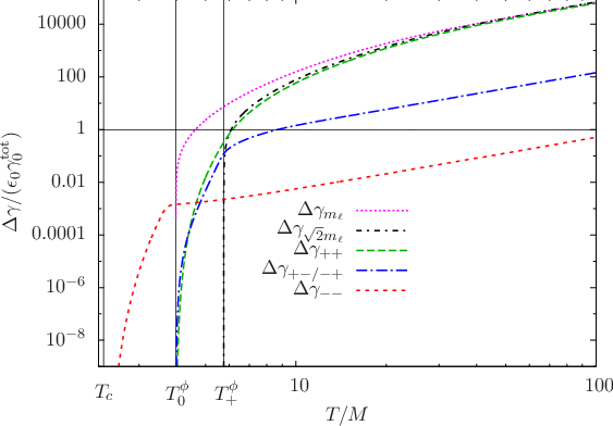
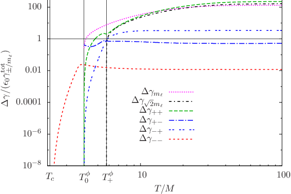
The ${C\!P}$ -asymmetries in Higgs boson decays at high temperature are shown in figure 4.8, normalised to $\epsilon_{0}\gamma^{\rm tot}$ and we have assumed that $M_{2}\gg M_{1},T$ . The behaviour is similar to the neutrino decays, where the ( $--$ )-asymmetry is strongly suppressed, while the ( $+-$ )-, the ( $-+$ )- and the ( $++$ )-asymmetries have a strict threshold at $T_{0}^{\phi}$ and are suppressed due to the reduced phase space between $T_{0}^{\phi}$ and $T_{+}^{\phi}$ , as expected. The ( $+-$ )- and ( $-+$ )- asymmetries are the same and are somewhat less suppressed than the $(++)$ -asymmetry between the thresholds $T_{0}^{\phi}$ and $T_{+}^{\phi}$ . In our approximation in the end of section 4.7, we have seen that the difference of the matrix elements $\Delta|\mathcal{M}|^{2}$ rises as $T^{2}$ , so $\Delta\gamma$ rises as $T^{4}$ , which can be seen in the plot for all finite-temperature asymmetries. The one-mode asymmetries $\Delta\gamma_{m_{\ell}}$ , $\Delta\gamma_{\sqrt{2}\,m_{\ell}}$ and the ( $++$ )-asymmetry are very close to each other at high temperature.

We also normalise the asymmetries to the corresponding decay rates in figure 4.9 and find that they all approach a constant value at high temperature, as is expected since the decay rates also rise as $T^{4}$ . The dents in the ratios $\Delta\gamma_{++}/(\epsilon_{0}\gamma_{+})$ and $\Delta\gamma_{+-}/(\epsilon_{0}\gamma_{+})$ with an external plus-mode lepton are similar to the ones for the neutrino decays and due to the very strong suppression of $\gamma_{+}$ below the threshold $T_{+}^{\phi}$ . The numerically dominant asymmetries $\Delta\gamma_{m_{\ell}}$ , $\Delta\gamma_{\sqrt{2}\,m_{\ell}}$ and $\Delta\gamma_{++}$ all settle at a rather high ${C\!P}$ -asymmetry, two orders of magnitude higher than at zero temperature, as we expect from our approximate calculation for a Higgs boson at rest at the end of section 4.7. This is partly due to a suppression of $|\mathcal{M}|^{2}$ which rises as $m_{\phi}^{2}=g_{\phi}^{2}T^{2}$ , but mainly due to the larger difference in matrix elements $\Delta|\mathcal{M}|^{2}$ for Higgs boson decays.

CHAPTER 5 Boltzmann Equations

Preliminary

In this chapter, we calculate the Boltzmann equations for leptogenesis. We include decays and inverse decays involving neutrinos, leptons and Higgs bosons. Concerning the scatterings, we argue that we can neglect all of them expect the on-shell contribution of the $\Delta L=2$ scatterings. We take into account thermal dispersion relations, but assume distributions close enough to equilibrium that we can use Boltzmann equations. For the distribution functions, we use the full quantum statistics, that is, Fermi-Dirac and Bose-Einstein statistics, but assume the kinetic equilibrium approximation $f_{i}=n_{i}/n_{i}^{\rm eq}f_{i}^{\rm eq}$ . It has been shown by reference [105] that this is a good approximation.

5.1 Particle Kinematics

The Boltzmann equations describe the time evolution of the distribution function of a particle species $\psi$ . We assume an isotropic and spatially homogeneous universe described by the Friedmann-Lemaitre-Robertson-Walker (FLRW) metric [72],

{\rm d}s^{2}={\rm d}t^{2}-a(t)^{2}\left\{\frac{{\rm d}r^{2}}{1-kr^{2}}+r^{2}{\rm d}\theta^{2}+r^{2}\sin^{2}\theta{\rm d}\phi^{2}\right\},

(5.1)

where $a(t)$ is the cosmic scale factor, which describes the expansion of the universe, $k=\pm 1,0$ specifies the curvature, and $(t,r,\theta,\phi)$ are the comoving coordinates.

The trajectory of a particle $\psi$ with mass $m_{\psi}\geq 0$ moving in a gravitational field is given by the geodesic equations of motion [113]:

	$\displaystyle\frac{{\rm d}p_{\psi}^{\mu}}{{\rm d}\tau}+\Gamma^{\mu}_{\nu\alpha}\,p_{\psi}^{\nu}\,p_{\psi}^{\alpha}$	$\displaystyle=0,$		(5.2)
	$\displaystyle\frac{{\rm d}x_{\psi}^{\mu}}{{\rm d}\tau}$	$\displaystyle=p_{\psi}^{\mu}.$		(5.3)

Since $s=m_{\psi}\tau$ is the eigen-time of the particle, $\tau$ is fixed and $p^{\mu}$ is the momentum of a particle $\psi$ .

In the FLRW metric the $\mu=0$ component of Eq (5.2) is given as

\displaystyle\frac{{\rm d}p_{\psi}^{0}}{{\rm d}\tau}+\frac{\dot{a}}{a}\mathbf{p}_{\psi}^{2}=0,\ \qquad\textrm{with}\quad\dot{a}=\frac{\partial a}{\partial t}.

(5.4)

Writing $p_{\psi}^{0}\,{\rm d}p_{\psi}^{0}=|\mathbf{p}_{\psi}|\,{\rm d}|\mathbf{p}_{\psi}|$ , this leads to:

⇔	$\displaystyle\|\dot{\mathbf{p}}_{\psi}\|a+\dot{a}\|\mathbf{p}_{\psi}\|=0$
$\displaystyle\Leftrightarrow$	$\displaystyle\frac{{\rm d}}{{\rm d}t}(\|\mathbf{p}_{\psi}\|a)=0$
$\displaystyle\Leftrightarrow$	$\displaystyle\|\mathbf{p}_{\psi}\|={\rm const.}\times\frac{1}{a}.$	(5.5)

Therefore the 3-momentum scales as $1/a$ .

In general, the Liouville operator describing the evolution of a point particle’s phase space in a gravitational field is given by

\displaystyle L=p^{\alpha}\frac{\partial}{\partial x^{\alpha}}-\Gamma{{}^{\alpha}_{\beta\gamma}}p^{\beta}p^{\gamma}\frac{\partial}{\partial p^{\alpha}}.

(5.6)

With this operator the equations of motion (5.2) and (5.3) can be written for the momentum as

\displaystyle\frac{{\rm d}p^{\mu}}{{\rm d}\tau}=L\left[p^{\mu}\right],

(5.7)

and for the space-time as

\displaystyle\frac{{\rm d}x^{\mu}}{{\rm d}\tau}=L\left[x^{\mu}\right].

(5.8)

Furthermore, the time derivative of the phase space distribution of a non-interacting gas vanishes,

\displaystyle\frac{{\rm d}f(x,p)}{{\rm d}\tau}=0.

(5.9)

Using the equations of motion for the particle we obtain the Boltzmann equations for the non-interacting particle species $\psi$ ,

\displaystyle L\left[f_{\psi}(x,p)\right]=0.

(5.10)

Since we are assuming a Robertson–Walker universe which is isotropic and homogeneous, the distribution function $f_{\psi}$ depends only on $t$ and $|\mathbf{p}_{\psi}|$ . Therefore, the Boltzmann equation can be written as [72]

\displaystyle L\left[f_{\psi}\right]=E_{\psi}\frac{\partial f_{\psi}}{\partial t}-H|\mathbf{p}_{\psi}|^{2}\frac{\partial f_{\psi}}{\partial E_{\psi}}=0,

(5.11)

where we have omitted arguments for the sake of notational clarity.

Since $p_{\psi}^{2}=m_{\psi}^{2}$ and because of the spatial isotropy of the Robertson–Walker–Metric, we have

\displaystyle|\mathbf{p}_{\psi}|^{2}\,\frac{\partial f_{\psi}}{\partial E_{\psi}}=E_{\psi}\,|\mathbf{p}_{\psi}|\,\frac{\partial f_{\psi}}{\partial|\mathbf{p}_{\psi}|}.

(5.12)

After dividing by $E_{\psi}$ , equation (5.11) has the form

\displaystyle L^{\prime}\left[f_{\psi}\right]=\frac{\partial f_{\psi}}{\partial t}-H\,|\mathbf{p}_{\psi}|\,\frac{\partial f_{\psi}}{\partial|\mathbf{p}_{\psi}|}.

(5.13)

Interactions are introduced on the right-hand side by a collision term $C\left[f_{\psi}\right]$ , which drives the distribution function towards its equilibrium value. The complete Boltzmann equation reads

\displaystyle L^{\prime}\left[f_{\psi}\right]=\frac{\partial f_{\psi}}{\partial t}-H\,|\mathbf{p}_{\psi}|\,\frac{\partial f_{\psi}}{\partial|\mathbf{p}_{\psi}|}=C\left[f_{\psi}\right].

(5.14)

Thus, the Boltzmann equation in a Robertson–Walker universe has the form of a partial differential equation. However, in the radiation dominated phase of the universe, in which leptogenesis takes place, equation (5.14) can be written as an ordinary differential equation by transforming to the dimensionless coordinates $z=m_{\psi}/T$ and $y_{\psi}=|\mathbf{p}_{\psi}|/T$ . Using the relation ${\rm d}T/{\rm d}t=-HT$ , the differential operator $\partial_{t}-|\mathbf{p}_{\psi}|H\partial_{|\mathbf{p}_{i}|}$ is written as $zH\partial_{z}$ , and consequently [114]

\displaystyle\frac{\partial f_{\psi}(z,y)}{\partial z}=\frac{z}{H(m_{\psi})}\,C_{D}\left[f_{\psi}(z,y)\right]

(5.15)

with $H\left(m_{\psi}\right)=H\left|{}_{T=m_{\psi}}\right.$ . In this form, the Boltzmann equation can be easily solved numerically on a grid for specific rescaled momenta $y$ . For the right hand side, we have to sum over the collision terms of all processes which involve the particle $\psi$ and change the phase space distribution. The collision term for a process $\psi+a+\cdots\leftrightarrow i+j+\cdots$ is given by[72]¹¹ 1 We have chosen a normalisation different from Kolb and Turner, so $C_{\textrm{here}}=\frac{1}{2E_{\psi}}C_{\rm KT}$

$\displaystyle g_{\psi}\,C[\psi+a+\cdots\leftrightarrow i+j+\cdots]$	$\displaystyle=-\frac{1}{2E_{\psi}}\int\prod_{\alpha}{\rm d}\tilde{p}_{\alpha}(2\pi)^{4}\delta^{4}(p_{\psi}+p_{a}+\cdots-p_{i}-p_{j}-\cdots)$
	$\displaystyle\times\left[\left\|\mathcal{M}(\psi+a+\cdots\rightarrow i+j+\cdots)\right\|^{2}f_{\psi}f_{a}\cdots(1\pm f_{i})(1\pm f_{j})\cdots\right.$
	$\displaystyle-\left.\left\|\mathcal{M}(i+j+\cdots\rightarrow\psi+a+\cdots)\right\|^{2}f_{i}f_{j}\cdots(1\pm f_{\psi})(1\pm f_{a})\cdots\right],$	(5.16)

where $\alpha=(a,\cdots,i,j,\cdots)$ ,

{\rm d}\tilde{p}_{\alpha}=\frac{{\rm d}^{3}p_{\alpha}}{(2\pi)^{3}2E_{\alpha}}.

(5.17)

The terms $(1\pm f_{i})$ hold for fermions ( $-$ ) and bosons ( $+$ ) and are interpreted as Fermi-blocking ( $-$ ) and Bose-enhancement ( $+$ ). In practice, we will only look at processes which involve three or four particles, that is, decays, inverse decays and scatterings. We have included the internal degrees of freedom, $g_{\psi},g_{a},\cdots,g_{i},g_{j},\cdots$ , in the matrix elements, therefore we need to put $g_{\psi}$ in front of the collision term since it is not included in the phase-space density $f_{\psi}$ .

We integrate equation (5.15) over the phase space of the incoming particle with $g_{\psi}\int{\rm d}^{3}p_{\psi}/(2\pi)^{3}$ and arrive at

\frac{{\rm d}n_{\psi}}{{\rm d}z}=-\frac{z}{H(m_{\psi})}\sum_{\rm processes}\left[\gamma(\psi+a+\cdots\rightarrow i+j+\cdots)-\gamma(i+j+\cdots\rightarrow\psi+a+\cdots)\right],

(5.18)

where

$\displaystyle\gamma(\psi+a+\cdots\rightarrow i+j+\cdots)$	$\displaystyle=-g_{\psi}\int\frac{{\rm d}^{3}p_{\psi}}{(2\pi)^{3}}C[\psi+a+\cdots\rightarrow i+j+\cdots]$
	$\displaystyle=\int\prod_{\beta}{\rm d}\tilde{p}_{\beta}(2\pi)^{4}\delta^{4}(p_{\psi}+p_{a}+\cdots-p_{i}-p_{j}-\cdots)$
	$\displaystyle\times\left\|\mathcal{M}(\psi+a+\cdots\rightarrow i+j+\cdots)\right\|^{2}f_{\psi}f_{a}\cdots(1\pm f_{i})(1\pm f_{j})\cdots,$	(5.19)

where we now integrate over $p_{\psi}$ as well, that is, $\beta=(\psi,a,\cdots,i,j,\cdots)$ . The analogous equation holds for $\gamma(i+j+\cdots\rightarrow\psi+a+\cdots)$ .

5.2 Low Temperature

5.2.1 Neutrino evolution

The Boltzmann equation for the evolution of the lightest right-handed neutrino is

	$\displaystyle\frac{{\rm d}n_{N_{1}}}{{\rm d}z}=-\frac{z}{H(M_{N_{1}})}$	$\displaystyle\left[\gamma(N_{1}\rightarrow\phi\ell_{+})+\gamma(N_{1}\to\bar{\phi}\bar{\ell}_{+})-\gamma(\phi\ell_{+}\to N_{1})-\gamma(\bar{\phi}\bar{\ell}_{+}\to N_{1})\right.$
	$\displaystyle+$	$\displaystyle\left.\gamma(N_{1}\rightarrow\phi\ell_{-})+\gamma(N_{1}\to\bar{\phi}\bar{\ell}_{-})-\gamma(\phi\ell_{-}\to N_{1})-\gamma(\bar{\phi}\bar{\ell}_{-}\to N_{1})\right]$		(5.20)

where $\ell_{\pm}$ denote the two lepton modes. We neglect scatterings since they are of higher order in the coupling constant. We will from now on omit the subscript 1 for the neutrino and write $N$ . The $CP$ -asymmetry in the matrix element is not relevant for neutrino decay, so we calculate the matrix element, which is the same for the above processes and define

\displaystyle\left|\mathcal{M}^{0}_{\pm}\right|^{2}\equiv\left|\mathcal{M}(N\to HL_{\pm})\right|^{2}=\left|\mathcal{M}(HL_{\pm}\to N)\right|^{2},

(5.21)

where now $HL_{\pm}$ denotes the sum of leptons and Higgs doublets, $\ell_{\pm}$ and $\phi$ , and their charge conjugated states $\bar{\ell}_{\pm}$ and $\bar{\phi}$ . The matrix elements are, however, different for the different lepton modes and also the momentum-conserving delta functions differ from each other. The subscript $\pm$ means ( $+$ ) or ( $-$ ), not the sum. When summing an expression $A_{\pm}$ that is dependent on the kind of lepton dispersion relation over the lepton modes, we write $\sum_{\pm}A_{\pm}$ . We have

\displaystyle\frac{{\rm d}n_{N}}{{\rm d}z}=-\frac{z}{H(M_{N_{1}})}\sum_{\pm}\left[\gamma(N\rightarrow HL_{\pm})-\gamma(HL_{\pm}\to N)\right]

(5.22)

For each of the two lepton modes, we have now

$\displaystyle\gamma(N\rightarrow HL_{\pm})-\gamma(HL_{\pm}\rightarrow N)$	$\displaystyle=\int{\rm d}\tilde{p}_{N}{\rm d}\tilde{p}_{L\pm}{\rm d}\tilde{p}_{H}(2\pi)^{4}\delta^{4}(p_{N}-p_{H}-p_{L\pm})$
	$\displaystyle\times\left[\left\|\mathcal{M}(N\rightarrow HL_{\pm})\right\|^{2}f_{N}(1+f_{H})(1-f_{L\pm})\right.$
	$\displaystyle-\left.\left\|\mathcal{M}(HL_{\pm}\rightarrow N)\right\|^{2}(1-f_{N})f_{H}f_{L\pm}\right].$	(5.23)

The term in square brackets in equation (5.23) reduces to

\left|\mathcal{M}^{0}_{\pm}\right|^{2}\left[f_{N}(1+f_{H})(1-f_{L\pm})-(1-f_{N})f_{H}f_{L\pm}\right]=\left|\mathcal{M}^{0}_{\pm}\right|^{2}\left[c_{N\rightarrow HL\pm}-c_{HL\pm\rightarrow N}\right],

(5.24)

where

	$\displaystyle c_{N\rightarrow HL\pm}$	$\displaystyle=f_{N}(1+f_{H})(1-f_{L\pm})\,,$
	$\displaystyle c_{HL\pm\rightarrow N}$	$\displaystyle=(1-f_{N})f_{H}f_{L\pm}\,.$		(5.25)

Throughout this chapter, we make the kinetic equilibrium assumption, that is, the phase space densities can be written as

f_{i}=\frac{n_{i}}{n_{i}^{\rm eq}}f_{i}^{\rm eq}=x_{i}f_{i}^{\rm eq},

(5.26)

where

\displaystyle x_{i}\equiv\frac{n_{i}}{n_{i}^{\rm eq}}\,,

(5.27)

where $n^{\rm eq}$ and $f^{\rm eq}$ are the equilibrium number densities and distributions. For the neutrino evolution, we can assume that the Higgs bosons are in equilibrium since they couple very strongly to the thermal bath, $f_{H}=f_{H}^{\rm eq}$ . The lepton distributions of the two modes are, strictly speaking, out of equilibrium since leptons and antileptons are created asymmetrically. However, the leptons are much closer to equilibrium than the neutrinos, so the neutrino evolution is not influenced by the lepton asymmetry. Therefore we approximate the lepton densities with their equilibrium density, $f_{L\pm}=f_{L\pm}^{\rm eq}$ . We will relax this assumption in the section on the lepton asymmetry evolution.

Using the relation

f_{N}^{\rm eq}(1+f_{H}^{\rm eq})(1-f_{L\pm}^{\rm eq})=(1-f_{N}^{\rm eq})f_{L\pm}^{\rm eq}f_{H}^{\rm eq},

(5.28)

we can write

	$\displaystyle c_{N\rightarrow HL\pm}$	$\displaystyle=x_{N}f_{N}^{\rm eq}(1+f_{H}^{\rm eq})(1-f_{L\pm}^{\rm eq})=(x_{N}-x_{N}f_{N}^{\rm eq})f_{H}^{\rm eq}f_{L\pm}^{\rm eq}\,,$
	$\displaystyle c_{HL\pm\rightarrow N}$	$\displaystyle=(1-x_{N}f_{N}^{\rm eq})f_{H}^{\rm eq}f_{L\pm}^{\rm eq}\,,$		(5.29)

and

\displaystyle c_{N\rightarrow HL\pm}-c_{N\rightarrow HL\pm}

\displaystyle=(x_{N}-1)f_{H}^{\rm eq}f_{L\pm}^{\rm eq}.

(5.30)

The decay densities are

$\displaystyle\gamma(N\rightarrow HL_{\pm})-\gamma(HL_{\pm}\rightarrow N)$	$\displaystyle=\int{\rm d}\tilde{p}_{N}{\rm d}\tilde{p}_{L\pm}{\rm d}\tilde{p}_{H}(2\pi)^{4}\delta^{4}(p_{N}-p_{H}-p_{L\pm})$
	$\displaystyle\times\left\|\mathcal{M}_{\pm}^{0}\right\|^{2}(x_{N}-1)f_{H}^{\rm eq}f_{L\pm}^{\rm eq}$
	$\displaystyle=(x_{N}-1)\gamma_{D\pm}^{N},$	(5.31)

where

\displaystyle\gamma_{D\pm}^{N}=\int{\rm d}\tilde{p}_{N}{\rm d}\tilde{p}_{L\pm}{\rm d}\tilde{p}_{H}(2\pi)^{4}\delta^{4}(p_{N}-p_{H}-p_{L\pm})\left|\mathcal{M}_{\pm}^{0}\right|^{2}f_{H}^{\rm eq}f_{L\pm}^{\rm eq}.

(5.32)

Note that $\gamma_{D\pm}^{N}$ is not the same as the equilibrium decay density in equation (3.42), but differs from the latter through the thermal factor $f_{H}f_{L}$ . It is an effective decay density, which enters the Boltzmann equations. The Boltzmann equation for the neutrinos reads

\displaystyle\frac{{\rm d}n_{N}}{{\rm d}z}=-\frac{z}{H(M_{N})}(x_{N}-1)\gamma_{D}^{N},

(5.33)

where $\gamma_{D}^{N}\equiv\gamma_{+}+\gamma_{-}$ , or, in analogy to equation (1.29),

\displaystyle\frac{{\rm d}n_{N}}{{\rm d}z}=-D^{N}(n_{N}-n_{N}^{\rm eq}),

(5.34)

where

\displaystyle D^{N}=\frac{\gamma_{D}^{N}}{n_{N}^{\rm eq}}\frac{1}{Hz}

(5.35)

and we have used $H(M_{N})=Hz^{2}$ . Most conveniently, the number densities are normalised by the entropy density $s$ in order to factorise their dependence on the expansion of the universe. The entropy density scales as

\displaystyle s=g_{*}\frac{2\pi^{2}}{45}T^{3},

(5.36)

where $g_{*}$ counts the total number of effectively massless degrees of freedom and is defined in equation (1.32). We define all number densities in terms of the entropy density as

\displaystyle Y_{i}\equiv\frac{n_{i}}{s},

(5.37)

then

\displaystyle x_{i}=\frac{Y_{i}}{Y_{i}^{\rm eq}}.

(5.38)

The Boltzmann equation reads

\displaystyle\frac{{\rm d}Y_{N}}{{\rm d}z}=-\frac{z}{sH_{1}}(x_{N}-1)\gamma_{D}^{N},

(5.39)

where

\displaystyle H_{1}\equiv H(T=M_{N})=\sqrt{\frac{4\pi^{3}g_{*}}{45}}\frac{M_{N}}{M_{\rm Pl}},

(5.40)

and the Planck mass is

\displaystyle M_{\rm Pl}=1.221\cdot 10^{19}\,{\rm GeV}.

(5.41)

5.2.2 Lepton asymmetry evolution

We set up evolution equations for the two different lepton modes separately and define the phase space density of the lepton asymmetry in the respective mode as

\displaystyle f_{\mathcal{L}h}=f_{\ell h}-f_{\bar{\ell}h}.

(5.42)

where $h=\pm 1$ denotes the helicity-over-chirality ratio of the leptons. The final lepton asymmetry is then $n_{\mathcal{L}}^{\rm fin}=n_{\mathcal{L}+}^{\rm fin}+n_{\mathcal{L}-}^{\rm fin}$ after evaluating the Boltzmann equations for each mode separately. The Boltzmann equations for leptons and antileptons read

$\displaystyle\frac{{\rm d}n_{\ell h_{1}}}{{\rm d}z}=-\frac{z}{H(M_{N})}\Big\{$	$\displaystyle\gamma(\ell_{h_{1}}\phi\rightarrow N)-\gamma(N\rightarrow\ell_{h_{1}}\phi)$
	$\displaystyle+\sum_{h_{2}}\left[\gamma(\ell_{h_{1}}\phi\rightarrow\bar{\ell}_{h_{2}}\bar{\phi})-\gamma(\bar{\ell}_{h_{2}}\bar{\phi}\rightarrow\ell_{h_{1}}\phi)\right]\Big\}\,,$
$\displaystyle\frac{{\rm d}n_{\bar{\ell}h_{1}}}{{\rm d}z}=-\frac{z}{H(M_{N})}\Big\{$	$\displaystyle\gamma(\bar{\ell}_{h_{1}}\bar{\phi}\rightarrow N)-\gamma(N\rightarrow\bar{\ell}_{h_{1}}\bar{\phi})$
	$\displaystyle+\sum_{h_{2}}\left[\gamma(\bar{\ell}_{h_{1}}\bar{\phi}\rightarrow\ell_{h_{2}}\phi)-\gamma(\ell_{h_{2}}\phi\rightarrow\bar{\ell}_{h_{1}}\bar{\phi})\right]\Big\},$	(5.43)

where we have $(h_{1},h_{2})=\pm 1$ to account for the second lepton involved in the scatterings and we have only included $\Delta L=2$ scatterings since the other scatterings involving neutrinos are negligible. For the evolution of the lepton asymmetry, we have

	$\displaystyle\frac{{\rm d}n_{\mathcal{L}h_{1}}}{{\rm d}z}=$	$\displaystyle-\frac{1}{Hz}\Big\{\gamma(\ell_{h_{1}}\phi\to N)-\gamma(\bar{\ell}_{h_{1}}\bar{\phi}\to N)-\gamma(N\to\ell_{h_{1}}\phi)+\gamma(N\to\bar{\ell}_{h_{1}}\bar{\phi})$
		$\displaystyle+\sum_{h_{2}}\left[\gamma(\ell_{h_{1}}\phi\to\bar{\ell}_{h_{2}}\bar{\phi})-\gamma(\bar{\ell}_{h_{1}}\bar{\phi}\to\ell_{h_{2}}\phi)+\gamma(\ell_{h_{2}}\phi\to\bar{\ell}_{h_{1}}\bar{\phi})-\gamma(\bar{\ell}_{h_{2}}\bar{\phi}\to\ell_{h_{1}}\phi)\right]\Big\}\,.$		(5.44)

At leading order in the couplings, the $\Delta L=2$ scatterings are computed at tree level and are consequently $CP$ -conserving. However, from these scatterings we must subtract the $CP$ -violating contribution where an on-shell $N_{1}$ is exchanged in the $s$ channel, shown in figure 5.1. This is because in the Boltzmann equations the process is already taken into account by inverse decays with successive decays, $\ell\phi\to N\to\bar{\ell}\bar{\phi}$ [115, 16, 116].

We must therefore replace the scattering rate by the subtracted rate,

\gamma(\ell_{h_{1}}\phi\to\bar{\ell}_{h_{2}}\bar{\phi})\to\gamma^{\rm sub}(\ell_{h_{1}}\phi\to\bar{\ell}_{h_{2}}\bar{\phi})\equiv\gamma(\ell_{h_{1}}\phi\to\bar{\ell}_{h_{2}}\bar{\phi})-\gamma^{\rm on-shell}(\ell_{h_{1}}\phi\to\bar{\ell}_{h_{2}}\bar{\phi})

(5.45)

and $\gamma(\bar{\ell}_{h_{1}}\bar{\phi}\to\ell_{h_{2}}\phi)$ accordingly, where $\gamma^{\rm on-shell}$ is the on-shell contribution. The Boltzmann equations then read

$\displaystyle\frac{{\rm d}n_{\mathcal{L}h_{1}}}{{\rm d}z}=$	$\displaystyle-\frac{1}{Hz}\Big\{\gamma(\ell_{h_{1}}\phi\to N)-\gamma(\bar{\ell}_{h_{1}}\bar{\phi}\to N)-\gamma(N\to\ell\phi_{h_{1}})+\gamma(N\to\bar{\ell}_{h_{1}}\bar{\phi})$
	$\displaystyle+\sum_{h_{2}}\big[\gamma^{\rm sub}(\ell_{h_{1}}\phi\to\bar{\ell}_{h_{2}}\bar{\phi})-\gamma^{\rm sub}(\bar{\ell}_{h_{1}}\bar{\phi}\to\ell_{h_{2}}\phi)$
	$\displaystyle+\gamma^{\rm sub}(\ell_{h_{2}}\phi\to\bar{\ell}_{h_{1}}\bar{\phi})-\gamma^{\rm sub}(\bar{\ell}_{h_{2}}\bar{\phi}\to\ell_{h_{1}}\phi)\big]\Big\}\,.$	(5.46)

Since the $CP$ -asymmetry in neutrino decays is defined on amplitude level as

\epsilon^{N}_{h}=\frac{\left|\mathcal{M}(N\to\phi\ell_{h})\right|^{2}-\left|\mathcal{M}(N\to\bar{\phi}\bar{\ell}_{h})\right|^{2}}{\left|\mathcal{M}(N\to\phi\ell_{h})\right|^{2}+\left|\mathcal{M}(N\to\bar{\phi}\bar{\ell}_{h})\right|^{2}}

(5.47)

and $\left|\mathcal{M}(N\to\phi\ell_{h})\right|^{2}+\left|\mathcal{M}(N\to\bar{\phi}\bar{\ell}_{h})\right|^{2}=\left|\mathcal{M}_{0h}\right|^{2}$ , we write

	$\displaystyle\left\|\mathcal{M}(N\to\phi\ell_{h})\right\|^{2}=\left\|\mathcal{M}(\bar{\phi}\bar{\ell}_{h}\to N)\right\|^{2}$	$\displaystyle=\frac{1+\epsilon_{h}^{N}}{2}\left\|\mathcal{M}_{0h}\right\|^{2},$
	$\displaystyle\left\|\mathcal{M}(N\to\bar{\phi}\bar{\ell}_{h})\right\|^{2}=\left\|\mathcal{M}(\phi\ell_{h}\to N)\right\|^{2}$	$\displaystyle=\frac{1-\epsilon_{h}^{N}}{2}\left\|\mathcal{M}_{0h}\right\|^{2}.$		(5.48)

It is useful to write the decay rates for the above $1\leftrightarrow 2$ processes as in section 5.2.1,

\gamma({\rm process})=\int\prod_{j}{\rm d}\tilde{p}_{j}(2\pi)^{4}\delta^{4}\left(\sum p_{j}\right)c({\rm process}),

(5.49)

where $p_{j}$ denotes the relevant momenta $p_{N}$ , $p_{\ell h}=p_{\bar{\ell}h}$ and $p_{\phi}=p_{\bar{\phi}}$ and $\delta^{4}(\sum p_{j})$ the momentum conservation $\delta^{4}(p_{N}-p_{\ell h}-p_{\phi})$ . The information about the specific process is encoded in $c({\rm process})$ and we have

$\displaystyle c_{N\to\ell_{h}\phi}$	$\displaystyle=\left\|\mathcal{M}(N\to\phi\ell_{h})\right\|^{2}f_{N}(1-f_{\ell h})(1+f_{\phi})$
$\displaystyle c_{\ell_{h}\phi\to N}$	$\displaystyle=\left\|\mathcal{M}(\phi\ell_{h}\to N)\right\|^{2}(1-f_{N})f_{\ell h}f_{\phi}$
$\displaystyle c_{N\to\bar{\ell}_{h}\bar{\phi}}$	$\displaystyle=\left\|\mathcal{M}(N\to\bar{\phi}\bar{\ell}_{h})\right\|^{2}f_{N}(1-f_{\bar{\ell}h})(1+f_{\bar{\phi}})$
$\displaystyle c_{\bar{\ell}_{h}\bar{\phi}\to N}$	$\displaystyle=\left\|\mathcal{M}(\bar{\phi}\bar{\ell}_{h}\to N)\right\|^{2}(1-f_{N})f_{\bar{\ell}h}f_{\bar{\phi}}.$	(5.50)

Since we are looking at the lepton asymmetry, the lepton distributions have to be out of equilibrium,

$\displaystyle f_{\ell/\bar{\ell}h}$	$\displaystyle=x_{\ell/\bar{\ell}h}f_{\ell h}^{\rm eq},$
$\displaystyle f_{\mathcal{L}h}$	$\displaystyle=x_{\mathcal{L}.h}f_{\ell h}^{\rm eq},$
$\displaystyle f_{\ell h}+f_{\bar{\ell}h}$	$\displaystyle\approx 2f_{\ell h}^{\rm eq},$	(5.51)

while the Higgs bosons can be assumed to be in equilibrium.

As explained in appendix E, the scattering rates can be written as

$\displaystyle\sum_{h_{f}}\left[\gamma^{\rm sub}(\ell_{h_{i}}\phi\right.$	$\displaystyle\left.\to\bar{\ell}_{h_{f}}\bar{\phi})-\gamma^{\rm sub}(\bar{\ell}_{h_{i}}\bar{\phi}\to\ell_{h_{f}}\phi)\right]$
	$\displaystyle=\sum_{h_{f}}\left[\gamma^{\rm sub}(\ell_{h_{f}}\phi\to\bar{\ell}_{h_{i}}\bar{\phi})-\gamma^{\rm sub}(\bar{\ell}_{h_{f}}\bar{\phi}\to\ell_{h_{i}}\phi)\right]=$
	$\displaystyle=\int{\rm d}\tilde{p}_{N}{\rm d}\tilde{p}_{\ell h_{i}}{\rm d}\tilde{p}_{\phi}(2\pi)^{4}\delta^{4}(p_{N}-p_{\ell h_{i}}-p_{\phi})\epsilon_{h_{i}}^{N}\left\|\mathcal{M}_{h_{i}}^{0}\right\|^{2}f_{\ell h_{i}}^{\rm eq}f_{\phi}^{\rm eq}(1-f_{N}^{\rm eq}).$	(5.52)

so we define²² 2 Note that our factor $c^{\rm sub}$ differs from reference [105], where they have the out-of-equilibrium distribution $(1-f_{N})$ instead of $(1-f_{N}^{\rm eq})$ . However, as derived in appendix E, we must employ $f_{N}^{\rm eq}$ , even if we had only one lepton mode, which also results in a Boltzmann equation for $(\ell-\bar{\ell})$ which is slightly different from theirs.

\displaystyle c^{\rm sub}_{h}=2\epsilon_{h}^{N}\left|\mathcal{M}^{0}_{h}\right|^{2}f_{\ell h}^{\rm eq}f_{\phi}^{\rm eq}(1-f_{N}^{\rm eq})

(5.53)

and calculate the integrand for the right-hand side of the Boltzmann equation (5.46),

	$\displaystyle c(N\to\ell_{h}\phi)-c(\ell_{h}\phi\to N)-$	$\displaystyle c(N\to\bar{\ell}_{h}\bar{\phi})+c(\bar{\ell}_{h}\bar{\phi}\to N)+c^{\rm sub}_{h}=$
		$\displaystyle=x_{\mathcal{L}h}f_{\ell h}^{\rm eq}(f_{\phi}^{\rm eq}+x_{N}f_{N}^{\rm eq})-2\epsilon_{h}^{N}f_{\ell h}^{\rm eq}f_{\phi}^{\rm eq}\left(x_{N}-1\right)\left(1-2f_{N}^{\rm eq}\right).$		(5.54)

We can easily check that this term vanishes when the neutrinos are in equilibrium, $x_{N}=1$ , and there is no previous lepton asymmetry, $x_{\mathcal{L}h}=0$ .

The Boltzmann equation reads now

\displaystyle\frac{{\rm d}n_{\mathcal{L}h}}{{\rm d}z}=-\frac{1}{Hz}\left[-\epsilon^{N}_{\gamma h}\gamma_{\epsilon h}^{N}\left(x_{N}-1\right)+\frac{x_{\mathcal{L}h}}{2}\left(\gamma_{Wh}^{N}+x_{N}\gamma_{Nh}^{N}\right)\right],

(5.55)

where $\gamma_{Wh}^{N}=\gamma_{Dh}^{N}$ is defined in equation (5.32) and

$\displaystyle\gamma_{\epsilon h}^{N}$	$\displaystyle=\int{\rm d}\tilde{p}_{N}{\rm d}\tilde{p}_{\ell h}{\rm d}\tilde{p}_{\phi}(2\pi)^{4}\delta^{4}(p_{N}-p_{\phi}-p_{\ell h})\left\|\mathcal{M}_{0}\right\|^{2}f_{\phi}^{\rm eq}f_{\ell h}^{\rm eq}(1-2f_{N}^{\rm eq})$
$\displaystyle\gamma_{Nh}^{N}$	$\displaystyle=\int{\rm d}\tilde{p}_{N}{\rm d}\tilde{p}_{\ell h}{\rm d}\tilde{p}_{\phi}(2\pi)^{4}\delta^{4}(p_{N}-p_{\phi}-p_{\ell h})\left\|\mathcal{M}_{0}\right\|^{2}f_{\ell h}^{\rm eq}f_{N}^{\rm eq},$
$\displaystyle\epsilon_{\gamma h}^{N}$	$\displaystyle=\frac{1}{\gamma_{\epsilon h}}\int{\rm d}\tilde{p}_{N}{\rm d}\tilde{p}_{\ell h}{\rm d}\tilde{p}_{\phi}(2\pi)^{4}\delta^{4}(p_{N}-p_{\phi}-p_{\ell h})\epsilon_{h}^{N}\left\|\mathcal{M}_{0}\right\|^{2}f_{\phi}^{\rm eq}f_{\ell h}^{\rm eq}(1-2f_{N}^{\rm eq}).$	(5.56)

We see that the rates and the ${C\!P}$ -asymmetries that enter the Boltzmann equations have slightly different thermal factors than the equilibrium rates and ${C\!P}$ -asymmetries in equations (3.42) and (4.69), which employ the factor $f_{N}(1-f_{\ell})(1+f_{\phi})$ for $N$ decays.

We may also write

\displaystyle\frac{{\rm d}Y_{\mathcal{L}h}}{{\rm d}z}=-\frac{z}{sH_{1}}\left[-\epsilon^{N}_{\gamma h}\gamma_{\epsilon h}^{N}\left(x_{N}-1\right)+\frac{x_{\mathcal{L}h}}{2}\left(\gamma_{Wh}^{N}+x_{N}\gamma_{Nh}^{N}\right)\right]

(5.57)

or, corresponding to equation (1.30),

\displaystyle\frac{{\rm d}n_{\mathcal{L}h}}{{\rm d}z}=\epsilon_{\gamma h}^{N}D_{\epsilon h}^{N}(n_{N}-n_{N}^{\rm eq})-(W_{0h}^{N}+W_{Nh}^{N}x_{N})n_{\mathcal{L}h},

(5.58)

where

$\displaystyle D_{\epsilon h}^{N}$	$\displaystyle=\frac{1}{Hz}\frac{\gamma_{\epsilon h}^{N}}{n_{N}^{\rm eq}}$
$\displaystyle W_{0h}$	$\displaystyle=\frac{1}{Hz}\frac{\gamma_{Wh}^{N}}{2n_{\ell h}^{\rm eq}}$
$\displaystyle W_{Nh}$	$\displaystyle=\frac{1}{Hz}\frac{\gamma_{Nh}^{N}}{2n_{\ell h}^{\rm eq}}.$	(5.59)

5.3 High temperature

As discussed in chapter 3, the neutrino processes $N\leftrightarrow\ell\phi$ are forbidden when the thermal masses of the Higgs bosons and leptons become too large, that is, when $m_{\phi}>M_{N}$ . However, new processes with the Higgs as single initial or final state are then allowed, $\phi\leftrightarrow N\ell$ . These are the dominant contributions to the neutrino and lepton evolution and they can be $CP$ -violating as well, so they contribute to generating a lepton asymmetry. We derive the Boltzmann equations for this high temperature regime in the following.

5.3.1 Neutrino evolution

We derive the Boltzmann equation analogously to section 5.2.1,

\displaystyle\frac{{\rm d}n_{N}}{{\rm d}z}=-\frac{1}{Hz}\sum_{h}\left[\gamma(NL_{h}\rightarrow H)-\gamma(H\rightarrow NL_{h})\right].

(5.60)

We have

$\displaystyle\gamma(NL_{h}\rightarrow H)-\gamma(H\rightarrow NL_{h})$	$\displaystyle=\int{\rm d}\tilde{p}_{N}{\rm d}\tilde{p}_{Lh}{\rm d}\tilde{p}_{H}(2\pi)^{4}\delta^{4}(p_{H}-p_{N}-p_{Lh})$
	$\displaystyle\times\left[\left\|\mathcal{M}(NL_{h}\rightarrow H)\right\|^{2}f_{N}f_{Lh}(1+f_{H})\right.$
	$\displaystyle-\left.\left\|\mathcal{M}(H\rightarrow NL_{h})\right\|^{2}(1-f_{N})(1-f_{Lh})f_{H}\right].$	(5.61)

The tree-level matrix elements $\left|\mathcal{M}^{0}_{h}\right|^{2}$ are the same at high temperature for the Higgs-processes, just the kinematics differ. So we have

\displaystyle\left|\mathcal{M}^{0}_{h}\right|^{2}\equiv\left|\mathcal{M}(NL_{h}\rightarrow H)\right|^{2}=\left|\mathcal{M}(H\rightarrow NL_{h})\right|^{2}.

(5.62)

Again, we assume the Higgs bosons and leptons to be in equilibrium. We write

\displaystyle\left|\mathcal{M}_{0}\right|^{2}\left[f_{N}f_{Lh}(1+f_{H})-(1-f_{N})(1-f_{Lh})f_{H}\right]=\left|\mathcal{M}_{0}\right|^{2}\left[c(NL_{h}\rightarrow H)-c(H\rightarrow NL_{h})\right]\,.

(5.63)

Using the relation

\displaystyle f_{N}^{\rm eq}f_{Lh}^{\rm eq}(1+f_{H}^{\rm eq})=(1-f_{N}^{\rm eq})(1-f_{Lh}^{\rm eq})f_{H}^{\rm eq},

(5.64)

we get

\displaystyle c(NL_{h}\rightarrow H)-c(H\rightarrow NL_{h})=(x_{N}-1)(1-f_{Lh}^{\rm eq})f_{H}^{\rm eq}.

(5.65)

The Boltzmann equation then reads

\displaystyle\frac{{\rm d}n_{N}}{{\rm d}z}=-\frac{1}{Hz}(x_{N}-1)\gamma_{D}^{\phi},

(5.66)

\displaystyle\frac{{\rm d}Y_{N}}{{\rm d}z}=-\frac{z}{sH_{1}}(x_{N}-1)\gamma_{D}^{\phi},

(5.67)

\displaystyle\frac{{\rm d}n_{N}}{{\rm d}z}=-D^{\phi}(n_{N}-n_{N}^{\rm eq}),

(5.68)

where $\gamma_{D}^{\phi}=\gamma_{D+}^{\phi}+\gamma_{D-}^{\phi}$ ,

\displaystyle\gamma_{Dh}^{\phi}=\int{\rm d}\tilde{p}_{N}{\rm d}\tilde{p}_{Lh}{\rm d}\tilde{p}_{H}(2\pi)^{4}\delta^{4}(p_{H}-p_{N}-p_{Lh})\left|\mathcal{M}^{0}_{h}\right|^{2}f_{H}^{\rm eq}(1-f_{Lh}^{\rm eq})

(5.69)

and

\displaystyle D^{\phi}=\frac{\gamma_{D}^{\phi}}{n_{N}^{\rm eq}}\frac{1}{Hz}\,.

(5.70)

5.3.2 Lepton asymmetry evolution

The Boltzmann equations for leptons and antileptons read

$\displaystyle\frac{{\rm d}n_{\ell h_{1}}}{{\rm d}z}=-\frac{1}{Hz}\Big\{$	$\displaystyle\gamma(\ell_{h_{1}}N\rightarrow\bar{\phi})-\gamma(\bar{\phi}\rightarrow\ell_{h_{1}}N)$
	$\displaystyle+\sum_{h_{2}}\left[\gamma(\ell_{h_{1}}\phi\rightarrow\bar{\ell}_{h_{2}}\bar{\phi})-\gamma(\bar{\ell}_{h_{2}}\bar{\phi}\rightarrow\ell_{h_{1}}\phi)\right]\Big\},$	(5.71)
$\displaystyle\frac{{\rm d}n_{\bar{\ell h_{1}}}}{{\rm d}z}=-\frac{z}{H(M_{N})}\Big\{$	$\displaystyle\gamma(\bar{\ell}_{h_{1}}N\rightarrow\phi)-\gamma(\phi\rightarrow\bar{\ell}_{h_{1}}N)$
	$\displaystyle+\sum_{h_{2}}\left[\gamma(\bar{\ell}_{h_{1}}\bar{\phi}\rightarrow\ell_{h_{2}}\phi)-\gamma(\ell_{h_{2}}\phi\rightarrow\bar{\ell}_{h_{1}}\bar{\phi})\right]\Big\},$	(5.72)

combined we get

	$\displaystyle\frac{{\rm d}n_{\mathcal{L}h_{1}}}{{\rm d}z}=$	$\displaystyle-\frac{1}{Hz}\Big\{\gamma(\ell_{h_{1}}N\to\bar{\phi})-\gamma(\bar{\ell}_{h_{1}}N\to\phi)-\gamma(\bar{\phi}\to\ell_{h_{1}}N)+\gamma(\phi\to\bar{\ell}_{h_{1}}N)$
		$\displaystyle+\sum_{h_{2}}\left[\gamma(\ell_{h_{1}}\phi\to\bar{\ell}_{h_{2}}\bar{\phi})-\gamma(\bar{\ell}_{h_{1}}\bar{\phi}\to\ell_{h_{2}}\phi)+\gamma(\ell_{h_{2}}\phi\to\bar{\ell}_{h_{1}}\bar{\phi})-\gamma(\bar{\ell}_{h_{2}}\bar{\phi}\to\ell_{h_{1}}\phi)\right]\Big\}\,.$		(5.73)

At high temperature, there can be no on-shell neutrino in the $s$ -channel of the $\Delta L=2$ scatterings, but there can be an on-shell neutrino exchange in the $u$ -channel as shown in figure 5.2.

Again, we need to subtract the $\Delta L=2$ rates since the $u$ -channel on-shell neutrino exchange corresponds to a Higgs decay followed by an inverse decay, $\ell\phi\to\ell N\bar{\ell}\to\bar{\phi}\bar{\ell}$ . We replace

\displaystyle\gamma(\ell_{h_{1}}\phi\to\bar{\ell}_{h_{2}}\bar{\phi})\to\gamma^{\rm sub}_{u}(\ell_{h_{1}}\phi\to\bar{\ell}_{h_{2}}\bar{\phi})\equiv\gamma(\ell_{h_{1}}\phi\to\bar{\ell}_{h_{2}}\bar{\phi})-\gamma^{\rm on-shell}_{u}(\ell_{h_{1}}\phi\to\bar{\ell}_{h_{2}}\bar{\phi})

(5.74)

and get

	$\displaystyle\frac{{\rm d}n_{\mathcal{L}h_{1}}}{{\rm d}z}=$	$\displaystyle-\frac{1}{Hz}\Big\{\gamma(\ell_{h_{1}}N\to\bar{\phi})-\gamma(\bar{\ell}_{h_{1}}N\to\phi)-\gamma(\bar{\phi}\to\ell_{h_{1}}N)+\gamma(\phi\to\bar{\ell}_{h_{1}}N)$
		$\displaystyle+\sum_{h_{2}}\left[\gamma^{\rm sub}(\ell_{h_{1}}\phi\to\bar{\ell}_{h_{2}}\bar{\phi})-\gamma^{\rm sub}(\bar{\ell}_{h_{1}}\bar{\phi}\to\ell_{h_{2}}\phi)+\gamma^{\rm sub}(\ell_{h_{2}}\phi\to\bar{\ell}_{h_{1}}\bar{\phi})-\gamma^{\rm sub}(\bar{\ell}_{h_{2}}\bar{\phi}\to\ell_{h_{1}}\phi)\right]\Big\}\,.$		(5.75)

We define the $CP$ -asymmetry in Higgs decays as

\displaystyle\epsilon_{h}^{\phi}\equiv\frac{\left|\mathcal{M}(\bar{\phi}\to N\ell_{h})\right|^{2}-\left|\mathcal{M}(\phi\to N\bar{\ell}_{h})\right|^{2}}{\left|\mathcal{M}(\bar{\phi}\to N\ell_{h})\right|^{2}+\left|\mathcal{M}(\phi\to N\bar{\ell}_{h})\right|^{2}},

(5.76)

thus

	$\displaystyle\left\|\mathcal{M}(\bar{\phi}\to N\ell_{h})\right\|^{2}=\left\|\mathcal{M}(\bar{\ell}_{h}N\to\phi)\right\|^{2}=\frac{1+\epsilon_{h}^{\phi}}{2}\left\|\mathcal{M}_{h}\right\|^{2},$
	$\displaystyle\left\|\mathcal{M}(\phi\to N\bar{\ell}_{h})\right\|^{2}=\left\|\mathcal{M}(\ell_{h}N\to\bar{\phi})\right\|^{2}=\frac{1-\epsilon_{h}^{\phi}}{2}\left\|\mathcal{M}_{h}\right\|^{2}\,.$		(5.77)

As explained in appendix E, the scattering rates are written as

$\displaystyle\sum_{h_{f}}\left[\gamma^{\rm sub}(\ell_{h_{i}}\phi\right.$	$\displaystyle\left.\to\bar{\ell}_{h_{f}}\bar{\phi})-\gamma^{\rm sub}(\bar{\ell}_{h_{i}}\bar{\phi}\to\ell_{h_{f}}\phi)\right]$
	$\displaystyle=\sum_{h_{f}}\left[\gamma^{\rm sub}(\ell_{h_{f}}\phi\to\bar{\ell}_{h_{i}}\bar{\phi})-\gamma^{\rm sub}(\bar{\ell}_{h_{f}}\bar{\phi}\to\ell_{h_{i}}\phi)\right]$
	$\displaystyle=\int{\rm d}\tilde{p}_{N}{\rm d}\tilde{p}_{\ell h_{i}}{\rm d}\tilde{p}_{\phi}(2\pi)^{4}\delta^{4}(p_{N}-p_{\ell h_{i}}-p_{\phi})\epsilon_{h}^{\phi}\left\|\mathcal{M}_{h_{i}}^{0}\right\|^{2}f_{\ell h_{i}}^{\rm eq}(1+f_{\phi}^{\rm eq})f_{N}^{\rm eq}\,,$	(5.78)

\displaystyle c_{h}^{\rm sub}=2\epsilon^{\phi}_{h}\left|\mathcal{M}_{h}^{0}\right|^{2}f_{\ell h}^{\rm eq}(1+f_{\phi}^{\rm eq})f_{N}^{\rm eq}

(5.79)

and we get for the right-hand side of equation (5.75),

	$\displaystyle c(\ell_{h}N\to\bar{\phi})-$	$\displaystyle c(\bar{\ell}_{h}N\to\phi)-c(\bar{\phi}\to\ell_{h}N)+c(\phi\to\bar{\ell}_{h}N)+c_{h}^{\rm sub}$
		$\displaystyle=x_{\mathcal{L}h}f_{\ell h}^{\rm eq}(f_{\phi}^{\rm eq}+x_{N}f_{N}^{\rm eq})+2\epsilon^{\phi}_{h}(1-f_{\ell h}^{\rm eq})f_{\phi}^{\rm eq}\left(x_{N}-1\right)\left(1-2f_{N}^{\rm eq}\right).$		(5.80)

The Boltzmann equation reads now

\displaystyle\frac{{\rm d}n_{\mathcal{L}h}}{{\rm d}z}=-\frac{1}{Hz}\left[-\epsilon_{\gamma h}^{\phi}\gamma_{\epsilon h}^{\phi}\left(x_{N}-1\right)+\frac{x_{\mathcal{L}h}}{2}\left(\gamma_{Wh}^{\phi}+x_{N}\gamma^{\phi}_{Nh}\right)\right],

(5.81)

where

$\displaystyle\gamma^{\phi}_{\epsilon h}$	$\displaystyle=\int{\rm d}\tilde{p}_{N}{\rm d}\tilde{p}_{\ell h}{\rm d}\tilde{p}_{\phi}(2\pi)^{4}\delta^{4}(p_{N}-p_{\phi}+p_{\ell h})\left\|\mathcal{M}_{h}^{0}\right\|^{2}f_{\phi}^{\rm eq}(1-f_{\ell h}^{\rm eq})(1-2f_{N}^{\rm eq})$
$\displaystyle\gamma_{Wh}^{\phi}$	$\displaystyle=\int{\rm d}\tilde{p}_{N}{\rm d}\tilde{p}_{\ell h}{\rm d}\tilde{p}_{\phi}(2\pi)^{4}\delta^{4}(p_{N}-p_{\phi}+p_{\ell h})\left\|\mathcal{M}_{h}^{0}\right\|^{2}f_{\phi}^{\rm eq}f_{\ell h}^{\rm eq}$
$\displaystyle\gamma^{\phi}_{Nh}$	$\displaystyle=\int{\rm d}\tilde{p}_{N}{\rm d}\tilde{p}_{\ell h}{\rm d}\tilde{p}_{\phi}(2\pi)^{4}\delta^{4}(p_{N}-p_{\phi}+p_{\ell h})\left\|\mathcal{M}_{h}^{0}\right\|^{2}f_{\ell h}^{\rm eq}f_{N}^{\rm eq},$
$\displaystyle\epsilon^{\phi}_{\gamma h}$	$\displaystyle=\frac{1}{\gamma^{\phi}_{\epsilon h}}\int{\rm d}\tilde{p}_{N}{\rm d}\tilde{p}_{\ell h}{\rm d}\tilde{p}_{\phi}(2\pi)^{4}\delta^{4}(p_{N}-p_{\phi}+p_{\ell h})\epsilon^{\phi}_{h}\left\|\mathcal{M}_{h}^{0}\right\|^{2}f_{\phi}^{\rm eq}(1-f_{\ell h}^{\rm eq})(1-2f_{N}^{\rm eq}).$	(5.82)

Analogous to equation (1.30), we may also write

\displaystyle\frac{{\rm d}n_{\mathcal{L}h}}{{\rm d}z}=-\epsilon^{\phi}_{\gamma h}D^{\phi}_{\epsilon h}(n_{N}-n_{N}^{\rm eq})-(W^{\phi}_{0h}+W^{\phi}_{Nh}x_{N})n_{\mathcal{L}h},

(5.83)

where

$\displaystyle D^{\phi}_{\epsilon h}$	$\displaystyle=\frac{1}{Hz}\frac{\gamma^{\phi}_{\epsilon h}}{n_{N}^{\rm eq}}$
$\displaystyle W^{\phi}_{0h}$	$\displaystyle=\frac{1}{Hz}\frac{\gamma^{\phi}_{Dh}}{2n_{\ell h}^{\rm eq}}$
$\displaystyle W^{\phi}_{Nh}$	$\displaystyle=\frac{1}{Hz}\frac{\gamma^{\phi}_{\mathcal{L}Nh}}{2n_{\ell h}^{\rm eq}}.$	(5.84)

Normalised by the entropy density, the equation reads

\displaystyle\frac{{\rm d}Y_{\mathcal{L}h}}{{\rm d}z}=-\frac{z}{sH_{1}}\left[-\epsilon_{\gamma h}^{\phi}\gamma_{\epsilon h}^{\phi}\left(x_{N}-1\right)+\frac{x_{\mathcal{L}h}}{2}\left(\gamma_{Wh}^{\phi}+x_{N}\gamma^{\phi}_{Nh}\right)\right].

(5.85)

5.4 Interacting Modes

The Boltzmann equations in the previous sections were derived under the assumption that the only interactions in which the leptons take part are the Yukawa interactions with Higgs bosons and heavy neutrinos, which have very small coupling constants $\lambda$ . This scenario would imply that the two modes only interact with each other via intermediate neutrinos or Higgs bosons, where the distributions and also the asymmetries in each mode are to first approximation decoupled. In a more realistic model, the lepton modes will couple to each other via the $SU(2)$ and $U(1)$ gauge bosons $W^{a}_{\mu}$ and $B_{\mu}$ in processes like $\ell_{\pm}\to\ell_{\mp}B$ . While it is conceptually interesting to consider the case that the two modes are completely decoupled, it might be more realistic to study the scenario where the interactions between the lepton modes are fast enough to keep them in chemical equilibrium.

Chemical equilibrium implies that for species that interact via processes $a+b\to i+j$ , the corresponding chemical potentials are related as

\displaystyle\mu_{a}+\mu_{b}=\mu_{i}+\mu_{j}\,.

(5.86)

When the processes which create or annihilate the particles and antiparticles of some species are fast, for example via $a+\bar{a}\to i+j$ , where $i$ and $j$ are in equilibrium and their chemical potentials vanish, then the chemical potentials of $a$ and $\bar{a}$ behave as

	$\displaystyle\mu_{a}+\mu_{\bar{a}}$	$\displaystyle=\mu_{i}+\mu_{j}=0\,,$
	$\displaystyle\Rightarrow\mu_{a}$	$\displaystyle=-\mu_{\bar{a}}\,.$		(5.87)

In order to derive the corresponding Boltzmann equation, we introduce a chemical potential $\mu_{h}$ for the lepton mode $\ell_{h}$ . For simplicity, we approximate the distribution with Maxwell-Boltzmann statistics, an approximation which is sufficient to derive the final Boltzmann equations. The distribution functions in kinetic equilibrium are

$\displaystyle f_{\ell h}(k)$	$\displaystyle={\rm e}^{-\beta(\omega_{h}-\mu_{h})}\,,$
$\displaystyle f_{\bar{\ell}h}(k)$	$\displaystyle={\rm e}^{-\beta(\omega_{h}+\mu_{h})}\,,$
$\displaystyle f_{\ell h}(k)-f_{\bar{\ell}h}(k)$	$\displaystyle={\rm e}^{-\beta\omega_{h}}({\rm e}^{\beta\mu_{h}}-{\rm e}^{-\beta\mu_{h}})\approx 2\beta\mu_{h}f_{\ell h}^{{\rm eq}}\,,$	(5.88)

for $\mu_{h}\ll T$ . We assume chemical equilibrium between the plus- and the minus-mode,

\displaystyle\mu_{+}=\mu_{-}\equiv\mu_{\ell}\,.

(5.89)

Moreover, we can make the approximation that the equilibrium densities are about the same since the thermal mass $m_{\ell}\approx 0.2\,T$ is too small to affect the momentum integration considerably in

	$\displaystyle n_{\ell_{h}}^{\rm eq}$	$\displaystyle=\int\frac{{\rm d}^{3}k}{(2\pi)^{3}}f_{\ell_{h}}^{\rm eq}(k)\,$
	$\displaystyle,\Rightarrow n_{\ell_{+}}^{\rm eq}$	$\displaystyle\approx n_{\ell_{-}}^{\rm eq}\approx n_{\ell,0}^{\rm eq}\,,$		(5.90)

where $n_{\ell,0}^{\rm eq}$ is the distribution for massless leptons. With these approximations, we have

$\displaystyle n_{\mathcal{L}_{+}}$	$\displaystyle=2\beta\mu_{\ell}n_{\ell_{0}}^{\rm eq}=n_{\mathcal{L}_{-}}\,,$
$\displaystyle n_{\mathcal{L}\pm}$	$\displaystyle\equiv n_{\mathcal{L}_{+}}+n_{\mathcal{L}_{-}}\equiv 2n_{\mathcal{L}_{h}}\,,$
$\displaystyle x_{\mathcal{L}\pm}$	$\displaystyle\equiv\frac{n_{\mathcal{L}\pm}}{n_{\ell 0}^{\rm eq}}\,,$	(5.91)

where the subscript $\pm$ indicates that we sum over the two modes, contrary to its use in the previous sections. We can now add the Boltzmann equations for the two modes in equations (5.57) and (5.85) and arrive at

\displaystyle\frac{{\rm d}Y_{\mathcal{L}\pm}}{{\rm d}z}=-\frac{z}{sH_{1}}\left[\Delta\gamma_{\pm}\left(x_{N}-1\right)+\frac{x_{\mathcal{L}\pm}}{4}\left(\gamma_{W\pm}+x_{N}\gamma_{N\pm}\right)\right],

(5.92)

where

$\displaystyle Y_{\mathcal{L}\pm}$	$\displaystyle=Y_{\mathcal{L}+}+Y_{\mathcal{L}-}\,,$
$\displaystyle\Delta\gamma_{\pm}$	$\displaystyle=\epsilon_{\gamma+}\gamma_{\epsilon+}+\epsilon_{\gamma-}\gamma_{\epsilon-}\,,$
$\displaystyle\gamma_{W\pm}$	$\displaystyle=\gamma_{W+}+\gamma_{W-}\,,$
$\displaystyle\gamma_{N\pm}$	$\displaystyle=\gamma_{N+}+\gamma_{N-}\,.$	(5.93)

The factor $1/4$ comes from the fact that $x_{\mathcal{L}h}=x_{\mathcal{L}\pm}/2$ . Depending on the temperature regime, we either have to employ the Higgs boson or the neutrino rates in the Boltzmann equations.

5.5 One-Mode Approximation

As we did in sections 3.2 and 4.7 for the decay rates and the ${C\!P}$ asymmetries, we also employ the one-mode approach for the Boltzmann equations. The equations are derived in analogy to sections 5.2 and 5.3 and read

	$\displaystyle\frac{{\rm d}Y_{N}}{{\rm d}z}$	$\displaystyle=-\frac{z}{sH_{1}}(x_{N}-1)\gamma_{Dm_{\ell}},$
	$\displaystyle\frac{{\rm d}Y_{\mathcal{L}}}{{\rm d}z}$	$\displaystyle=-\frac{z}{sH_{1}}\left[-\Delta\gamma_{m_{\ell}}\left(x_{N}-1\right)+\frac{x_{\mathcal{L}}}{2}\left(\gamma_{Wm_{\ell}}+x_{N}\gamma_{Nm_{\ell}}\right)\right],$		(5.94)

where $\gamma_{Dm_{\ell}}$ , $\gamma_{Wm_{\ell}}$ , $\gamma_{Nm_{\ell}}$ and $\Delta\gamma_{m_{\ell}}$ are defined in equations (5.32), (5.56), (5.69) and (5.82) and one has to make the appropriate replacements for the matrix elements and the lepton dispersion relations of the one-mode approach for $m_{\ell}$ and $\sqrt{2}\,m_{\ell}$ .

5.6 Evaluation of the Boltzmann Equations

We solve the Boltzmann equations for five different scenarios:

1.

the zero temperature case with Maxwell-Boltzmann statistics,
2.

the two-lepton-mode approach where the two modes do not interact with each other,
3.

the two-mode approach where the modes couple strongly to each other,
4.

the one-mode approach for a thermal mass $m_{\ell}$ ,
5.

and the one-mode approach for an asymptotic thermal mass $\sqrt{2}\,m_{\ell}$ .

In the decoupled case, the lepton asymmetries for the plus- and the minus-mode evolve separately from each other. When solving the equations, one has to specify the initial conditions for the neutrino abundance and the lepton asymmetry. We assume a vanishing initial lepton asymmetry and distinguish between three cases for the neutrino abundances:

1.

Zero initial abundance: this is the case, for example, when an inflaton field decays mostly into SM particles and not into the heavy neutrinos.
2.

Thermal initial abundance: this can be realised when some additional interactions keep the neutrinos in equilibrium at $T\gg M_{1}$ , for example via a heavy $Z^{\prime}$ boson related to $SO(10)$ unification [117].
3.

Dominant initial abundance: this is the case, for example, when an inflaton decays predominantly into $N_{1}$ .

The coupling $(\lambda^{\dagger}\lambda)_{11}$ , which enters the neutrino decay rate, is parameterised by the so-called decay parameter $K$ , defined as

\displaystyle K\equiv\frac{\widetilde{m}_{1}}{m^{*}}\,,

(5.95)

where $\widetilde{m}_{1}$ and $m^{*}$ are the effective neutrino mass and the so-called equilibrium neutrino mass, defined in equations (1.27) and (1.28). The case $K>1$ is called strong washout regime and the case $K<1$ weak washout regime.

We want to analyse the evolution of the neutrino abundance and lepton asymmetries for the weak and strong washout regimes and different initial abundances. To this end, we write the Boltzmann equations for the different scenarios in the form of equations (5.34), (5.58), (5.68) and (5.83),

	$\displaystyle\frac{{\rm d}Y_{N}}{{\rm d}z}$	$\displaystyle=-D(Y_{N}-Y_{N}^{\rm eq})\,.$
	$\displaystyle\frac{{\rm d}Y_{\mathcal{L}}}{{\rm d}z}$	$\displaystyle=\epsilon_{0}D_{\epsilon}(Y_{N}-Y_{N}^{\rm eq})-(W+W_{N}x_{N})Y_{\mathcal{L}}\,,$		(5.96)

where

	$\displaystyle D$	$\displaystyle=\frac{z}{H_{1}}\frac{\gamma_{D}}{sY_{N}^{\rm eq}}\,,$	$\displaystyle D_{\epsilon}$	$\displaystyle=\frac{z}{H_{1}}\frac{\Delta\gamma}{\epsilon_{0}sY_{N}^{\rm eq}}\,,$
	$\displaystyle W$	$\displaystyle=\frac{z}{H_{1}}\frac{\gamma_{W}}{2sY_{\mathcal{L}}^{\rm eq}}\,,\quad$	$\displaystyle W_{N}$	$\displaystyle=\frac{z}{H_{1}}\frac{\gamma_{N}}{2sY_{\mathcal{L}}^{\rm eq}}\,.$		(5.97)

One usually refers to $D_{\epsilon}(Y_{N}-Y_{N}^{\rm eq})$ as source term since this term is responsible for the production of a lepton asymmetry. The term $(W+W_{N}x_{N})Y_{\mathcal{L}}^{\rm eq}$ is called washout term since it usually has the opposite sign as the source term and reduces the production of the lepton asymmetry. The terms $D$ , $D_{\epsilon}$ , $W$ and $W_{N}$ are different for the different scenarios. Note that for the finite temperature cases, $D_{\epsilon}$ is not the same as $D$ and there is an additional washout term $W_{N}$ due to the quantum statistics. Our analysis closely follows the arguments and explanations in reference [116] and the interested reader will find a comprehensive explanation of leptogenesis dynamics in the vacuum case therein.

5.6.1 Weak washout for zero initial abundance

Let us start with the weak washout regime and zero initial abundance. We define a value $z_{\rm eq}$ by the condition

\displaystyle Y_{N}(z_{\rm eq})=Y_{N}^{\rm eq}(z_{\rm eq})\,.

(5.98)

For $z\ll 1$ , the neutrino abundance is negligible compared to $Y_{N}^{\rm eq}$ ,

\displaystyle\frac{{\rm d}Y_{N}}{{\rm d}z}\simeq DY_{N}^{\rm eq}\,,

(5.99)

where $Y_{N}^{\rm eq}$ is approximately constant for $z\ll 1$ . The entropy density $s$ is proportional to $z^{-3}$ and $\gamma_{D}$ is proportional to $z^{-2}$ in vacuum and $z^{-4}$ for the Higgs boson decays at high temperature in the finite temperature cases. Thus $D\sim z^{2}$ in the vacuum case and $D\sim{\rm const.}$ at finite temperature. Neglecting $Y_{N}^{\rm initial}$ and $z^{\rm initial}$ , the integration yields $Y_{N}\simeq zD(z)/3\sim z^{3}$ for the vacuum case and $Y_{N}\simeq zD\sim z$ for the finite temperature cases. We show the numerical results for $K=0.005$ and zero initial abundance in figures 5.3 and 5.4, where these power laws for $Y_{N}(z)$ can be observed for $z\lesssim 0.1$ . We also see that $Y_{N}^{m_{\ell}}>Y_{N}^{\sqrt{2}\,m_{\ell}}>Y_{N}^{\pm}\gg Y_{N}^{0}$ , which reflects $\gamma_{D}^{m_{\ell}}>\gamma_{D}^{\sqrt{2}\,m_{\ell}}>\gamma_{D}^{\pm}\gg\gamma_{0}$ . Between the thresholds $z_{+}^{\phi}$ and $z_{+}^{N}$ , the finite-temperature abundances do not evolve much, which reflects that the decay rates are very low or vanishing in this regime. The neutrino abundance for the asymptotic mass $\sqrt{2}\,m_{\ell}$ does not rise at all at high temperature, while $Y_{N}^{m_{\ell}}$ rises slightly between $z_{0}^{\phi/N}$ and $z_{+}^{\phi/N}$ , where the rate is non-zero. The two-mode rate $\gamma_{\pm}$ is, though very suppressed, present over the whole threshold range between $z_{+}^{\phi}$ and $z_{+}^{N}$ due to the minus-modes, so $Y_{N}^{\pm}$ rises slightly. At low temperature, $z>z_{\rm eq}$ , the neutrino abundances of the different scenarios are very close to each other, since for $z\gtrsim 2$ , the rates are very close to the vacuum rate, $\gamma_{D,W,N}^{T>0}\simeq\Delta\gamma^{T>0}/\epsilon_{0}\simeq\gamma_{0}$ . In this regime, $Y_{N}$ is much larger than $Y_{N}^{\rm eq}$ since the coupling is too small to keep the abundance close to equilibrium.

Having outlined the evolution of the neutrino abundance at high temperature, we can understand the evolution of the lepton asymmetry at high temperature. The washout term in the Boltzmann equations proportional to $Y_{\mathcal{L}}$ is much smaller than the source term $D_{\epsilon}(Y_{N}-Y_{N}^{\rm eq})$ , since $Y_{\mathcal{L}}/\epsilon_{0}\ll Y_{N}^{\rm eq}$ , and we have for $z\ll z_{\rm eq}$ ,

	$\displaystyle Y_{\mathcal{L}}^{T>0}$	$\displaystyle\simeq-z\epsilon_{0}D_{\epsilon}\,$
	$\displaystyle Y_{\mathcal{L}}^{T=0}$	$\displaystyle\simeq-z\epsilon_{0}\frac{D_{\epsilon}(z)}{3}\,.$		(5.100)

In the high temperature regime, the lepton asymmetry is negative and follows the neutrino abundance in its absolute value,

\displaystyle Y_{\mathcal{L}}(z)\simeq-\epsilon_{0}\frac{D_{\epsilon}}{D}Y_{N}(z)=-\frac{\Delta\gamma}{\gamma_{D}}Y_{N}(z)\,.

(5.101)

For the vacuum case, $D_{\epsilon}\equiv D$ and $Y_{\mathcal{L}}/\epsilon_{0}\simeq-Y_{N}$ , while for the finite temperature cases, $D_{\epsilon}/D=\Delta\gamma/(\epsilon_{0}\gamma_{D})\sim\mathcal{O}(10^{1})$ .³³ 3 We saw in chapter 4 that $\Delta\gamma/(\epsilon_{0}\gamma_{D})\sim\mathcal{O}(10^{2})$ at high temperature instead of $\mathcal{O}(10^{1})$ . The discrepancy is due to rates and asymmetries that occur in the Boltzmann equations and that are slightly different from the usual rates and ${C\!P}$ -asymmetries in chapters 3 and 4 due to the different statistical factors they employ, for example $1$ or $(1-2f_{N}^{\rm eq})$ instead of the usual factor $(1-f_{N}^{\rm eq})$ . See the discussion in section 4.5.3 and compare the thermal factors in equations (3.43) and (5.69). Both behaviours can be observed in figures 5.3 and 5.4. The lepton asymmetry in the minus-mode obeys the same power law as the other finite-temperature modes, but is about a factor $100$ lower due to the lower rates. The combined ( $\pm$ )-abundance closely follows the plus-abundance since the influence of the minus-mode rates is very suppressed and also the different washout term with factor $1/4$ instead of $1/2$ can be neglected.

Before turning to the intermediate temperatures $z\sim z_{\rm eq}$ , let us discuss the low temperature regime. For $z>z_{\rm eq}$ , $Y_{N}\gg Y_{N}^{\rm eq}$ , so the source term dominates and washout can be neglected. Since in this regime, $D_{\epsilon}^{T>0}\simeq D^{T>0}\simeq D^{T=0}$ , we can write

\displaystyle\frac{{\rm d}Y_{\mathcal{L}}}{{\rm d}z}\simeq\epsilon_{0}D(Y_{N}-Y_{N}^{\rm eq})=-\epsilon\frac{{\rm d}Y_{N}}{{\rm d}z}\,.

(5.102)

To first order, the negative lepton asymmetry created below $z_{\rm eq}$ and the positive contribution from above $z_{\rm eq}$ have the same magnitude and cancel each other. For the remaining asymmetry that did not cancel, the washout contribution up to $z_{\rm eq}$ and the exact behaviour of the abundances around $z_{\rm eq}$ are crucial.

Assuming that $Y_{N}(z=\infty)=0$ , we get

\displaystyle Y_{\mathcal{L}}^{\rm fin}\simeq\epsilon_{0}Y_{N}(z_{\rm eq})-|Y_{\mathcal{L}}(z_{\rm eq})|\,,

(5.103)

so we see that the evolution of the difference $\Delta Y(z)\equiv Y_{N}(z)-|Y_{\mathcal{L}}(z)|/\epsilon_{0}$ below $z_{\rm eq}$ is crucial for the final lepton asymmetry. For the regime $1\lesssim z\lesssim z_{\rm eq}$ , we can write

	$\displaystyle\frac{{\rm d}\Delta Y}{{\rm d}z}$	$\displaystyle\simeq Y_{N}^{\rm eq}(D-D_{\epsilon})\,,$
	$\displaystyle D-D_{\epsilon}$	$\displaystyle=\frac{z}{H_{1}}\frac{1}{sY_{N}^{\rm eq}}\left(\gamma_{D}-\frac{\Delta\gamma}{\epsilon}\right)\,.$		(5.104)

For the finite-temperature cases, the ${C\!P}$ -asymmetry in the decay rates, $\Delta\gamma/\epsilon_{0}$ , is considerably smaller than the decay rate $\gamma_{D}$ in the range $z_{0}^{N}\lesssim z\lesssim 2$ , which can be seen in figure 4.7. Moreover, for the one-mode cases, $\Delta\gamma_{m}/\epsilon_{0}$ approaches $\gamma_{m}$ faster than $\Delta\gamma_{++}$ approaches $\gamma_{+}$ for the plus-mode. Above $z_{+}^{N}$ , the ratio $\Delta\gamma/(\epsilon_{0}\gamma_{D})$ for the two one-mode cases is about the same. Thus, the difference $\Delta D\equiv D-D_{\epsilon}$ is largest for the two-mode approach, smaller and about the same for the two one-mode approaches and vanishing for the vacuum approach, $\Delta D^{+}>\Delta D^{m_{\ell}}\simeq\Delta D^{\sqrt{2}\,m_{\ell}}$ and $\Delta D^{0}=0$ . As a result, $\Delta Y^{+}\gtrsim\Delta Y^{m_{\ell}}\simeq\Delta Y^{\sqrt{2}\,m_{\ell}}$ at $z_{\rm eq}$ and therefore the final asymmetries are related as $Y_{\mathcal{L}}^{+}>Y_{\mathcal{L}}^{m_{\ell}}\simeq Y_{\mathcal{L}}^{\sqrt{2}\,m_{\ell}}\gg Y_{\mathcal{L}}^{0}$ . Note that the final asymmetry is non-vanishing for the vacuum case, since the washout at higher temperature is larger than at lower temperature due to the larger decay rate. For the finite temperature cases, the difference $D-D_{\epsilon}$ bin the crucial regime $z\simeq z_{\rm eq}$ governs the final asymmetry.

The evolution of the decoupled minus-mode at low temperature is very different but not hard to understand. The asymmetry rises at $z\gtrsim z_{+}^{N}$ , because this is the regime above $z_{c}$ where $\Delta\gamma_{-+}$ is maximal and therefore $D_{\epsilon}^{-}$ is maximal as well. Between the thresholds $z_{+}^{\phi}$ and $z_{+}^{N}$ , $\Delta\gamma_{-+}$ is suppressed by the internal plus-lepton and $\Delta\gamma_{--}$ is suppressed by the residue of the internal minus-lepton, so $D_{\epsilon}$ is negligible and $Y_{\mathcal{L}}^{-}$ does not rise. Above $z\sim 1$ , $\Delta\gamma_{-+}$ falls due to the residue of the external minus-mode and $Y_{\mathcal{L}}^{-}$ does not change. The final lepton asymmetry therefore does not change its sign above $z\gtrsim z_{\rm eq}$ and keeps the value it achieves at around $1\lesssim z\lesssim 2$ where the ${C\!P}$ -asymmetry $\Delta\gamma_{-+}$ becomes small.

The combined ( $\pm$ )-mode does not evolve differently from the plus-mode since the influence from the $\gamma^{-}$ rates can be neglected and also the washout term with the additional factor $1/2$ is not noticeable since washout is very small in all temperature regimes. Summarising, there are four differing lepton asymmetries in this regime: the vacuum case, the $m_{\ell}$ -case, the ( $+$ )-case and the ( $-$ )-case. The $\sqrt{2}\,m_{\ell}$ -case yields the same asymmetry as the $m_{\ell}$ -case and the ( $\pm$ )-case yields the same asymmetry as the ( $+$ )-case. We show the four differing lepton asymmetries together in figure 5.5.

5.6.2 Strong and intermediate washout for zero initial abundance

For strong washout, the evolution of the neutrino abundance is analogous to the weak washout regime, with $Y_{N}^{T}\sim z$ and $Y_{N}^{0}\sim z^{3}$ , as shown in figures 5.6 and 5.7. The couplings are stronger, therefore the abundances rise faster and meet $Y_{N}^{\rm eq}$ earlier at $z_{\rm eq}\sim 1$ . For larger $z$ , the couplings are strong enough to keep $Y_{N}$ close to equilibrium. The evolution of the lepton asymmetry is nicely explained in reference [116] for the vacuum case with some rather accurate analytical approximations. In this work, we are only interested in the difference of the vacuum case to the finite temperature case. In the strong washout regime, the lepton asymmetries rise rather fast and the washout term, which competes with the source term, becomes larger than the latter at some temperature $z_{\rm min}$ , where the lepton asymmetry reaches its most negative value. The source term becomes small when $Y_{N}$ approaches its equilibrium value, so the washout term drives the asymmetry evolution back to zero. At $z\gtrsim z_{\rm eq}$ , the neutrino abundance slightly overshoots $Y_{N}^{\rm eq}$ , so the source term changes sign and adds to the washout term until the lepton asymmetry becomes positive, where the washout term changes its sign as well and is competing again. At low temperature, source term and washout term have the same magnitude when the lepton asymmetry reaches a maximum at $z_{\rm max}$ . Above $z_{\rm max}$ , the lepton asymmetry is again driven to zero by the larger washout. At very low temperature, washout and source term become very small and do not influence the asymmetry further, which settles at a final value $Y_{\mathcal{L}}^{\rm fin}$ . We see that in the strong washout regime, the dynamics are governed by the washout term. The evolution of the finite temperature lepton asymmetries is analogous to the vacuum case, but they settle to a different final value. For the finite temperature cases, the equilibrium density of leptons is smaller than in the vacuum case due to the thermal mass $m_{\ell}\sim 0.2\,T$ . The washout term is effectively larger than for the vacuum case and competes with the source term in a stronger way. Therefore, the asymmetry evolution appears slightly damped compared to the vacuum case and the final asymmetry is marginally lower. The evolution of the minus-mode is analogous to the evolution at weak washout, rises fast below $z_{+}^{\phi}$ and does not change above the thresholds since $Y_{N}\sim Y_{N}^{\rm eq}$ in this regime. The combined ( $\pm$ )-mode tracks the plus-mode until washout becomes relevant at $z\gtrsim z_{\rm eq}$ . The washout term for the ( $\pm$ )-mode is always about a factor two smaller than for the plus-mode, since we add the minus- and plus-washout rates, where the minus-rate is always negligible compared to the plus-rate. Thus, the ( $\pm$ )-abundance is less affected by washout, so the dynamics are affected by the source term in a stronger way and the final asymmetry is larger. We can view this behaviour as always distributing half the asymmetry in a mode $\ell_{-}$ which couples strongly to $\ell_{+}$ and is not affected by washout. The final asymmetry is about a factor two larger than for the other scenarios in the strong washout regime.

The case of intermediate washout is shown in figure 5.8, where we only show the two-mode cases since in this regime, the final lepton asymmetries of the one-mode cases are the same as for the plus-mode. The dynamics can be viewed as an interpolation between the strong and weak washout regimes and the final asymmetries are very similar to each other.

5.6.3 Non-zero initial abundance

We also present the dynamics for thermal and dominant initial abundance in figures 5.9–5.14.

For weak washout and thermal initial abundance, $Y_{N}\gg|Y_{\mathcal{L}}|$ for low temperatures, and according to equation (5.103), $Y_{\mathcal{L}}^{\rm final}/\epsilon_{0}\sim Y_{N}^{\rm initial}$ . For weak washout and dominant initial abundance, this equation holds as well, as can be seen in figures 5.9 and 5.10. For intermediate washout $K\sim 1$ and dominant abundance, shown in figures 5.11 and 5.12, the lepton asymmetry production is stopped between the thresholds for the thermal cases and the production above $z\sim 1$ does not succed in producing an asymmetry as high as in the vacuum case. For the ( $\pm$ )-case, the asymmetry production is larger since it is not as much affected by washout.

For the strong washout regime and large initial neutrino abundances, the dynamics at high temperature are interesting, as shown in figures 5.13 and 5.14, but the interplay between source term and washout term at low temperature governs the final asymmetry as in the zero-abundance case. We reproduce the well-known fact that the initial conditions do not influence the final asymmetry in the strong washout regime, while the arguments concerning the equilibrium distribution of leptons with thermal mass and the reduced washout of the ( $\pm$ )-mode still hold and lead to the same lepton asymmetry as for zero initial abundance. The decoupled minus-mode is very much affected by the coupling, that is the decay parameter $K$ , and the initial conditions, since the final lepton asymmetry is produced at high temperatures. The stronger the coupling, the larger the asymmetry production of the minus-mode at high temperatures and the larger the final value. Moreover, the larger the initial deviation of the neutrino abundance from equilibrium, the larger the asymmetry production and the final asymmetry. The final lepton asymmetry in this mode is thus lowest for neutrinos with thermal initial abundance.

5.6.4 Final lepton asymmetries

The values of the final asymmetries are shown in figures 5.15–5.17 for different initial abundances.

For zero initial abundance and weak washout, shown in figure 5.15, the asymmetry for the finite-temperature cases are larger than for the vacuum case by about one order of magnitude due to the difference of the thermal rates $\gamma_{D}$ and the ${C\!P}$ -asymmetries $\Delta\gamma$ at $z\gtrsim z_{+}^{N}$ . The lepton asymmetry for the plus-mode is also slightly larger than for the one-mode cases due to a suppression of the ${C\!P}$ asymmetry compared to the one-mode approaches. For strong washout, the asymmetry production in the vacuum case is marginally more efficient than in the thermal cases due to a smaller lepton equilibrium distribution, while the lepton asymmetry in the ( $\pm$ )-approach is by a factor $2$ larger than in the other cases since half of the asymmetry is in the $\ell_{-}$ -modes and not affected by washout. The minus-mode is completely decoupled, the lepton asymmetry bears the opposite sign as the other lepton asymmetries and rises with stronger couplings, that is with larger decay parameter $K$ . As discussed in section 5.4, this scenario might not be realistic since the modes will couple to each other via gauge bosons, so an evolution similar to the ( $\pm$ )-case seems more likely.

For thermal initial abundance and weak washout, shown in figure 5.16, the final asymmetry equals the equilibrium abundance $Y_{\mathcal{L}}/\epsilon_{0}$ , while in the strong washout regime, it shows the same behaviour as in the case of zero initial neutrino abundance. The minus-mode asymmetry is very low for thermal initial neutrino abundance since the neutrinos are close to equilibrium at high temperatures. Contrary to the zero initial abundance case, it bears the same sign as the lepton asymmetries of the other scenarios.

For dominant initial abundance, shown in figure 5.17, the final asymmetries assume their maximal value in the weak washout regime, when the coupling is weak enough not to wash them out at low temperature. For larger couplings $K\sim 1$ , the thresholds lead to a halted asymmetry production for the finite temperature cases and not as much asymmetry can be produced as for the vacuum case. The ( $\pm$ )-case shows a larger asymmetry compared to the other thermal cases due to the weaker washout. At strong coupling $K\gg 1$ , the asymmetries are the same as for thermal and zero initial neutrino abundance. The minus-mode asymmetry is large in all washout regimes, since the neutrinos are far from equilibrium at high temperatures when the $\ell_{-}$ -asymmetry is produced.

A summary of the several initial conditions can be seen in figure 5.18, where we have omitted the $\sqrt{2}\,m_{\ell}$ case since it is very close to the $m_{\ell}$ case in all scenarios. In the weak washout regime, the case with zero initial abundance is most strongly affected by thermal corrections which amount to one order of magnitude, and the plus-mode asymmetry is additionally enhanced by a factor of about two. In the intermediate regime, the dominant-initial-abundance case is influenced very much by thermal corrections. Therefore, a production mechanism for dominant neutrino abundance has to take into account such thermal effects. In the strong washout regime, one would naturally expect that thermal corrections can be neglected. We see that this is not the case since for strongly interacting leptonic quasiparticles, a part of the lepton asymmetry can be hidden in the $\ell_{-}$ -mode which is unaffected by washout, thus producing an asymmetry by up to a factor of two larger than at zero temperature. The effect of the thermal lepton mass on the equilibrium distribution of the leptons is an interesting feature, but very small and can be neglected for all practical purposes.

Conclusions

We see this work as a contribution to the revived quest for calculating and capturing effects that the finite density and temperature of the medium has on early universe dynamics. For a minimal and self-consistent toy model of leptogenesis, which consists only of neutrinos, leptons and Higgs bosons, we have performed an extensive analysis of the effects of HTL corrections. This implies capturing the effects of thermal masses, modified dispersion relations and modified helicity structures. We put special emphasis on the influence of the two fermionic quasiparticles, which show a different behaviour than particles in vacuum, notably through their dispersion relations, but also the helicity structure of their interactions. Our work is thus similar to the work done in reference [16], where the authors of the latter work did not include the effects of fermionic quasiparticles and get a different result for the ${C\!P}$ -asymmetries, which are crucial for the evolution of the lepton asymmetry. Our toy model produces two lepton asymmetries stored in the two different lepton modes without the possibility of an equilibration of these asymmetries by SM processes. Since we expect the lepton modes to interact via gauge bosons in the bath, we examine a second case where the modes are strongly coupled to each other. As a third and fourth case, we approximate the lepton propagators by zero temperature propagators with the zero temperature mass replaced by the thermal lepton mass in one case and the asymptotic mass in the other case. We refer to these cases as one-mode approach. All four thermal cases are compared to the zero-temperature case.

Our analysis proceeded in three steps: Calculating interaction rates, calculating the necessary ${C\!P}$ -asymmetries and deriving and solving the corresponding Boltzmann equations. We calculated the decay rates in chapter 3. Thermal decay rates in the context of leptogenesis have been calculated using vacuum states as external states and replacing the zero-temperature mass by the respective thermal mass[16]. We calculated the decay rates with the full HTL-dependence via the neutrino self-energy and the optical theorem. While for scalars, that is the Higgs bosons in our case, this gives the same result as inserting thermal masses in the kinematics, the results for fermions are somewhat different, both conceptually and numerically. Neglecting the zero-temperature fermion mass, the resummation of HTL fermion self-energies results in an effective fermion propagator that does not break chiral invariance and is split up in two helicity modes. The external fermion states therefore behave conceptually different from the ones with chirality-breaking thermal masses that have been inserted in the kinematics by hand. Moreover, one has to take care of one additional mode, which has implications for the Boltzmann equations.

In order to understand and describe the behaviour of the modes, we have assigned momentum-dependent quasi-masses to them in section 2.5.2. Numerically, the presence of the two modes with momentum-dependent masses leads to different thresholds corresponding to the asymptotic masses of the two modes, $\sqrt{2}\,m_{\ell}$ and zero mass, and the zero momentum mass $m_{\ell}$ . It is a well known fact, that for large temperatures, the thermal mass of the Higgs boson becomes so large that neutrino decays are no longer allowed, but rather the Higgs bosons decay into neutrinos and leptons. While reference [16] finds that decays are possible above or below their respective thresholds, we find that the decay into the negative mode is always possible, while the decay into the plus-mode is possible up to the thresholds corresponding to the thermal mass $m_{\ell}$ , but becomes suppressed by the reduction of possible lepton momenta at the thresholds with the asymptotic mass $\sqrt{2}\,m_{\ell}$ . From pure kinematical arguments, one would expect the one-mode rate with the asymptotic mass to be a much better approximation to the plus-rate than the one-mode rate for the thermal mass. The fact that this is not the case shows the importance of the helicity structure of the leptonic quasiparticles, which suppresses the rate for the plus-mode such that it is much lower than $\gamma_{\sqrt{2}\,m_{\ell}}$ . For the Higgs boson decays at high temperature, the thresholds are analogous to the neutrino decays at low temperature. We observe the same $T^{4}$ -proportionality for Higgs boson decays as reference [16].

We calculated the ${C\!P}$ -asymmetries in chapter 4. To our knowledge, this is the first correct calculation of a ${C\!P}$ -asymmetry in leptogenesis that includes HTL-corrections.⁴⁴ 4 Reference[16] has an incorrect calculation for the ${C\!P}$ -asymmetry of the neutrino and Higgs decays with HTL corrections in the propagators and thermal masses in the external states. The discrepancy is discussed in detail in reference[23]. The authors of the first reference get a factor $1-f_{\ell^{\prime}}+f_{\phi^{\prime}}-2f_{\ell^{\prime}}f_{\phi^{\prime}}$ for the neutrino decays and $f_{\phi^{\prime}}-f_{\ell^{\prime}}-2f_{\phi^{\prime}}f_{\ell^{\prime}}$ for the Higgs boson decays due to an erroneous choice of cutting rules in the real time formalism. The correct calculation gives $1-f_{\ell^{\prime}}+f_{\phi^{\prime}}$ for the neutrino decays and $f_{\phi^{\prime}}+f_{\ell^{\prime}}$ for the Higgs boson decays. This discrepancy is also responsible for our ${C\!P}$ -asymmetry in Higgs decays being a factor ten larger than their result. We present rules for the product of spinors that are related to the fermionic quasiparticles in equations (4.14) and (4.15) and derive frequency sums for the HTL fermion propagator in equation (4.33). We find four different ${C\!P}$ -asymmetries corresponding to the four different choices of lepton modes both in the loop and as external states. We find the ${C\!P}$ -asymmetry to be symmetric under an exchange of the lepton mode in the loop and the external lepton mode, such that $\Delta\gamma_{+-}=\Delta\gamma_{-+}$ . At finite temperature, there are three possible cuttings for the vertex contribution, the $\{\ell^{\prime},\phi^{\prime}\}$ -cut that corresponds to zero temperature and two additional cuts involving the internal $N^{\prime}$ , namely through $\{N^{\prime},\ell^{\prime}\}$ and $\{N^{\prime},\phi^{\prime}\}$ , which have been found by [16, 21, 96] and examined more closely in [22], using the real-time formalism. We obtain the same cuts using the imaginary time formalism and concentrate on the $\{\ell^{\prime},\phi^{\prime}\}$ -cut, assuming the hierarchical limit of $M_{2}\gg M_{1}$ . As expected from the zero-temperature result, we find the vertex contribution proportional to the self-energy contribution in this limit. Contrary to reference [16], we find that the ${C\!P}$ -asymmetry in Higgs boson decays is larger than the asymmetry in neutrino decays by about a factor of $100$ if appropriately normalised. This is due to a suppression of the Higgs boson decay rate and a thermal enhancement of the ${C\!P}$ -asymmetry by the distribution functions of the Higgs bosons and leptons. We compare the ${C\!P}$ -asymmetries in the two-mode approach to the ${C\!P}$ -asymmetries in the one-mode approach. We find that for the two-mode approach, the helicity structure of the modes prohibits the two leptons to be scattered strictly in the same direction while for the one-mode approach, this direction is only mildly suppressed. Notably this fact is responsible for suppressing the ( $++$ )- ${C\!P}$ -asymmetry compared to the asymmetries of the one-mode approach, as well as the residues of the plus-modes to less extent.

We derive and evaluate the Boltzmann equations for our approaches in chapter 5, performing the crucial subtraction of on-shell intermediate states in appendix E⁵⁵ 5 The thermal factor $(1-f_{N}^{\rm eq})$ we find is different from the factor $(1-f_{N})$ that reference [105] uses, where they employ the out-of equilibrium distribution function for neutrinos without deriving their result explicitly.. We compare the results of the Boltzmann equations for our five cases, that is, decoupled lepton modes, strongly coupled lepton modes, the one-mode approach with $m_{\ell}$ , the one-mode approach with $\sqrt{2}\,m_{\ell}$ , and the vacuum case. We assume three different initial values for the abundance of neutrinos: zero, thermal and dominant abundance, motivated by different scenarios for the production of heavy neutrinos after inflation [16]. In the weak washout regime, we find that using thermal masses enhances the final lepton asymmetry by about one order of magnitude for zero initial neutrino abundance. This is due to the fact that the ${C\!P}$ -asymmetry and the decay rate evolve differently at $z\gtrsim 1$ when using thermal masses, since the ${C\!P}$ -asymmetry suffers from an additional suppression by thermal masses through the leptons and Higgs bosons in the loop. Due to the helicity structure of the modes, the ${C\!P}$ -asymmetry of the plus-mode is additionally suppressed, which results in an additional enhancement of the plus-mode lepton asymmetry compared to the final asymmetries of the one-mode approaches. The enhancement we find is similar to the one found in reference [16] in this regime, but hard to compare quantitatively due to their different approach which includes scatterings and the discrepancy in the ${C\!P}$ -asymmetry. In the strong washout regime, thermal masses do not show an influence as expected⁶⁶ 6 There is a slight suppression of the lepton asymmetry for thermal masses, since the thermal mass suppresses the equilibrium distribution of the leptons somewhat and thereby enhances the washout term.. However, when we couple the plus- and minus-mode strongly, we observe an enhancement of the lepton asymmetry by a factor of about two, since we stored half of the asymmetry in a mode that essentially does not interact with the neutrinos and is therefore not affected by washout. For intermediate washout, that is $K\sim 1$ , we find that the lepton asymmetries with thermal masses are about one magnitude lower than in the vacuum case when we assume dominant initial neutrino abundance. This is due to the fact that the lower ${C\!P}$ -asymmetry does not succeed in producing as much lepton asymmetry at $z\gtrsim 1$ when using thermal masses. A decoupled minus-mode would show a behaviour completely different from the other thermal cases and the vacuum case for all initial values of the neutrino abundance. The lepton asymmetry in such a decoupled mode is produced mainly at high temperature and only slightly affected by the development at $z\gtrsim 1$ , where it decouples from the evolution of the other abundances. Therefore, the washout parameter $K$ , which determines the coupling strength and thereby the asymmetry production at high temperatures, is crucial for the final value of the lepton asymmetry in this mode, as is the initial neutrino abundance.

Summarising, we argue that for an accurate description of medium effects on leptogenesis, the influence of thermal quasiparticles, notably the effects of the two fermionic modes, cannot be neglected. Similar to reference [16], our study shows that thermal masses have a strong effect in the weak washout regime, while the effect of fermionic modes has an additional influence on the final lepton asymmetry in this regime. We also showed that notably in the strong washout regime, the presence of a quasi-sterile lepton mode that is not affected by washout can have a non-negligible effect on the final lepton asymmetry. Future studies should clarify the dynamics of the interaction between the two fermionic modes and determine whether the evolution of the asymmetries in the two modes is closer to the decoupled or the strongly coupled case.

Another important aspect that might be studied in future works is the influence of the finite width of the fermionic modes [118], notably the minus-mode. Such effects could be studied using Kadanoff-Baym equations [95, 96, 97, 98, 23, 21, 19, 17, 20, 99, 100] or some other formalism that takes into account non-equilibrium quantum effects. In the quest for a unified description of finite-temperature effects on leptogenesis, it is important to include SM interactions in the Kadanoff-Baym studies that are under way. To this end, quasiparticle excitations of fermions and gauge-bosons should be taken into account. Last but not least, the fermionic modes might have an influence on other related dynamics in the early universe that involve fermions, such as thermal production of axions, axinos or gravitinos. Notably our introduction of sum rules for quasiparticle spinors in equations (4.14) and (4.15), as well as the derivation of frequency sums in equation (4.33) can be a valuable contribution to future calculations.

Future experimental results from the neutrino sector and from high-temperature dynamics, such as RHIC or observations at the LHC, will provide interesting input for these theoretical efforts. Whatever the outcome of such future experiments and calculations, the quest for a sufficiently complete and unified description of the influence of the hot, dense medium on early-universe dynamics, such as leptogenesis or the production of dark matter particles, is guaranteed to remain an attractive and vibrant field of research with much insight to be gained both from theoretical and experimental side.

Appendix A Green’s Functions at Zero Temperature

We consider the case of a scalar field $\phi(x)$ with mass $m$ , where $x\equiv(x_{0},{\bf x})$ , $x_{0}\equiv t$ , we are using natural units $\hbar=c=k_{B}=1$ and are in the relativistic regime where we use the Minkowski metric $x^{2}=x_{\mu}x^{\mu}=g_{\mu\nu}x^{\nu}x^{\mu}=x_{0}^{2}-{\bf x}^{2}$ . The amplitude of a particle to travel from $x$ to $y$ if $x_{0}<y_{0}$ or from $y$ to $x$ if $y_{0}<x_{0}$ is called Feynman propagator and is equal to the two-point correlation function defined as

{\rm i}\,\Delta_{F}(x-y)\equiv\langle 0|T\{\phi(x)\phi(y)\}|0\rangle\,,

(A.1)

where $T$ denotes the time ordering operator which acts on two fields as

T\{\phi(x)\phi(y)\}=\left\{\begin{matrix}\;\phi(x)\phi(y)&&x_{0}>y_{0}&\\ \phi(y)\phi(x)&&x_{0}<y_{0}&\end{matrix}\right.\,.

(A.2)

We can express the scalar field by its Fourier transform

\phi(x)=\left.\int\frac{{\rm d^{3}}k}{(2\pi)^{3/2}}\frac{1}{(2\omega_{k})^{1/2}}[a({\bf k}){\rm e}^{-{\rm i}\,K\cdot x}+a^{\dagger}({\bf k}){\rm e}^{\,{\rm i}\,K\cdot x}]\right|_{k_{0}=\omega_{k}}\,,

(A.3)

where $K\equiv(k_{0},{\bf k})$ is the four-momentum of the field, $\omega_{k}\equiv\sqrt{{\bf k}^{2}+m^{2}}$ the energy and the Fourier coefficients represent creation $a({\bf k})$ and destruction operators $a^{\dagger}({\bf k})$ , which create or destroy a boson with momentum $\bf k$ . They act on a state $|n({\bf k})\rangle$ with $n$ particles of momentum $\bf k$ as

	$\displaystyle a({\bf k})\|n({\bf k})\rangle$	$\displaystyle=$	$\displaystyle\sqrt{n({\bf k})}\;\|n({\bf k})-1\rangle$		(A.4)
	$\displaystyle a^{\dagger}({\bf k})\|n({\bf k})\rangle$	$\displaystyle=$	$\displaystyle\sqrt{n({\bf k})+1}\;\|n({\bf k})+1\rangle\,,$		(A.5)

in particular $a({\bf k})|0\rangle=0$ for all $\bf k$ .

Using the Fourier representation of $\phi$ , the Feynman propagator can be written as

\Delta_{F}(x-y)=\int\frac{{\rm d}^{4}K}{(2\pi)^{4}}\frac{{\rm e}^{-{\rm i}\,K\cdot(x-y)}}{K^{2}-m^{2}+{\rm i}\,\epsilon}\,,

(A.6)

where the term $+{\rm i}\,\epsilon$ accounts for the so-called Feynman prescription, that is in the complex $k_{0}$ -plane we integrate above the pole at $k_{0}=\omega_{k}$ and below the pole at $k_{0}=-\omega_{k}$ . When we carry out the $k_{0}$ -integration, we find for $x_{0}>y_{0}$

\Delta_{F}(x-y)=-{\rm i}\,\left.\int\frac{{\rm d}^{3}k}{(2\pi)^{3}}\frac{1}{2\omega_{k}}{\rm e}^{-{\rm i}K\cdot(x-y)}\right|_{k_{0}=\omega_{k}}\,.

(A.7)

Appendix B Analytic Solution of the Dispersion Relations for HTL Fermions

The dispersion relations of the two lepton modes are given by the poles of the corresponding propagator. Hence, we seek the zeros of

D_{\pm}(K)=\Delta_{\pm}(K)^{-1}=\left[-k_{0}\pm k+\frac{m_{\ell}^{2}}{k}\left(\pm 1-\frac{\pm k_{0}-k}{2k}\ln\frac{k_{0}+k}{k_{0}-k}\right)\right]^{-1}

(B.1)

The equations $D_{\pm}=0$ can be transformed by the substitutions

$\displaystyle x_{+}$	$\displaystyle:=\frac{k_{0}+k}{k_{0}-k}$	(B.2)
$\displaystyle x_{-}$	$\displaystyle:=\frac{k_{0}-k}{k_{0}+k}=\frac{1}{x_{+}}$	(B.3)
$\displaystyle c$	$\displaystyle:=\frac{k^{2}}{m_{\ell}^{2}}.$	(B.4)

This yields

D_{\pm}=\pm\frac{k}{c}\frac{1}{x_{\pm}-1}\left(-2c-1+x_{\pm}-\ln x_{\pm}\right).

(B.5)

Further introducing

s:=-\exp(-2c-1)

(B.6)

leads to

D_{\pm}=\frac{\mp 2k}{1+\ln(-s)}\frac{1}{x_{\pm}-1}\left[x_{\pm}+\ln(-s)-\ln x_{\pm}\right].

(B.7)

Since the prefactor does not have poles for the values of $K$ we are looking at, solving $D_{\pm}=0$ amounts to solving

x_{\pm}+\ln(-s)-\ln x_{\pm}=0,

(B.8)

which in turn means

s=-x_{\pm}\epsilon^{-x_{\pm}}.

(B.9)

This is the defining equation of the Lambert W function [119, 120], thus the solution reads

x_{\pm}=-W(s).

(B.10)

According to the definition in Eq. (B.6)

-1/\epsilon\leq s\leq 0,

(B.11)

thus the two real branches of the Lambert function, $W_{0}$ and $W_{-1}$ , correspond to the two solutions we seek. In the range given by Eq. (B.11) $W_{0}\geq-1$ and $W_{-1}\leq-1$ . For $k_{0}\geq k$ we have $x_{+}\geq 1$ and $x_{-}\leq 1$ . Hence, the physical solutions for $x_{\pm}$ read

x_{+}=-W_{-1}(s)\hskip 28.45274pt{\rm and}\hskip 28.45274ptx_{-}=-W_{0}(s).

(B.12)

The corresponding results for $\omega_{\pm}$ are then given by

	$\displaystyle\omega_{+}$	$\displaystyle=k\;\frac{W_{-1}(s)-1}{W_{-1}(s)+1}$		(B.13)
	$\displaystyle\omega_{-}$	$\displaystyle=-k\;\frac{W_{0}(s)-1}{W_{0}(s)+1}.$		(B.14)

Making use of the relations [121]

W_{0,-1}(z)+\ln(W_{0,-1}(z))=\ln z,

(B.15)

one can directly prove the result by plugging Eqs. (B.13) and (B.14) into Eq. (B.1).

Appendix C Quantities at Zero Temperature

C.1 Decay Rate at Zero Temperature

We know that at $T=0$ , the decay rate of a heavy neutrino with definite spin at rest is given by

\Gamma_{\rm rf}(N\to\phi\ell)=\frac{(\lambda^{\dagger}\lambda)_{jj}}{16\pi}M_{j}\,,

(C.1)

where we have not summed over neutrino spins. Then

\Gamma_{D}=\frac{M_{j}}{E}\Gamma_{\rm rf}=\frac{M_{j}}{E}\frac{(\lambda^{\dagger}\lambda)_{jj}}{16\pi}M_{j}

(C.2)

and the decay density for definite neutrino spin is

$\displaystyle\gamma_{D}(N\to\phi\ell)$	$\displaystyle=$	$\displaystyle\frac{1}{2\pi^{2}}\int_{M_{j}}^{\infty}{\rm d}EEpf_{N}\Gamma_{D}$	(C.3)
	$\displaystyle=$	$\displaystyle\frac{(\lambda^{\dagger}\lambda)_{jj}}{4(2\pi)^{3}}M_{j}^{2}\int_{M_{j}}^{\infty}{\rm d}Epf_{N}$	(C.4)
	$\displaystyle=$	$\displaystyle\frac{(\lambda^{\dagger}\lambda)_{jj}}{4(2\pi)^{3}}M_{j}^{3}TK_{1}\left(\frac{M_{j}}{T}\right),$	(C.5)

where $K_{1}(z)$ is a Bessel function of second kind and $z=M_{j}/T$ .

C.2 $\boldsymbol{C\!P}$ -Asymmetry at Zero Temperature

For the ${C\!P}$ -asymmetry at zero temperature, the integrals are the same as for $T>0$ , just the thermal masses are zero and the lepton propagator is

S_{\ell}^{\prime}=\frac{\not{K^{\prime}}}{K^{\prime 2}},

(C.6)

so the spin sum is

\frac{1}{2}\sum_{r,s}(\overline{u}_{\ell}P_{R}u_{N})(\overline{u}_{N}P_{R}S_{\ell}^{\prime}P_{L}u_{\ell})=M_{j}K^{\mu}K^{\prime}_{\mu}\Delta_{\ell}^{\prime},

(C.7)

where

\Delta_{\ell}^{\prime}=\frac{1}{K^{\prime 2}}\,,

(C.8)

and we have averaged over the neutrino degrees of freedom. At zero temperature, we can use the Cutkosky rules to compute discontinuities, so we replace propagators by $\delta$ -functions. There are three possible cuttings, however, the cuttings which involve $N_{2}$ correspond to a process where one massless particle decays into $N_{2}$ and the other massless particle which is not possible kinematically. The only possible cutting is through the Higgs boson and lepton propagator, so

	$\displaystyle\Delta_{\ell}^{\prime}\rightarrow-2\pi{\rm i}\delta(K^{\prime 2}),$		(C.9)
	$\displaystyle\Delta_{\phi}^{\prime}\rightarrow-2\pi{\rm i}\delta(Q^{\prime 2}).$		(C.10)

We get

	$\displaystyle{\rm Im}(I_{0}I_{1}^{*})$	$\displaystyle=$	$\displaystyle-\frac{{\rm i}}{2}{\rm Disc}(I_{0}I_{1}^{*})=-\frac{1}{2}M_{j}M_{k}{\rm Disc}\left(\int\frac{{\rm d}^{4}k^{\prime}}{(2\pi)^{4}}\Delta_{N}^{\prime}\Delta_{\phi}^{\prime}\Delta_{\ell}^{\prime}K_{\mu}K^{\prime\mu}\right)$		(C.11)
		$\displaystyle=$	$\displaystyle\frac{M_{j}M_{k}}{16\pi}\left[1-\left(1+x\right)\ln\frac{1+x}{x}\right],$		(C.12)

where

x=\frac{M_{k}^{2}}{M_{j}^{2}}\,.

(C.13)

Analogously, we get for the self-energy

{\rm Im}(I_{0}I_{1}^{*})=\frac{M_{j}M_{k}}{16\pi}\frac{1}{1-x}\,.

(C.14)

The CP-Asymmetry at zero temperature reads

\epsilon=\frac{1}{8\pi}\frac{{\rm Im}[(\lambda^{\dagger}\lambda)_{jk}^{2}]}{(\lambda^{\dagger}\lambda)_{jj}}g(x)\,,

(C.15)

where

\displaystyle g(x)=\sqrt{x}\left[\frac{1}{1-x}+1-\left(1+x\right)\ln\frac{1+x}{x}\right]\,.

(C.16)

C.3 Boltzmann Equations at Zero Temperature

We can derive the Boltzmann equations for the neutrino and lepton evolution at zero temperature, approximating the phase-space densities with Maxwell-Boltzmann distributions,

\displaystyle f_{i}(E_{i})=\exp(-E_{i}\beta)\,,

(C.17)

where energy conservation in scatterings and decays implies

\displaystyle f_{N}

\displaystyle=f_{L}f_{H}\,

(C.18)

and there are no Higgs decays at high temperature. For the neutrino evolution, we get, analogous to equation (5.39),

\displaystyle\frac{{\rm d}Y_{N}}{{\rm d}z}=-\frac{z}{sH_{1}}(x_{N}-1)\gamma_{0},

(C.19)

where

\displaystyle\gamma_{0}=\int{\rm d}\tilde{p}_{N}{\rm d}\tilde{p}_{L}{\rm d}\tilde{p}_{H}(2\pi)^{4}\delta^{4}(p_{N}-p_{H}-p_{L})\left|\mathcal{M}_{0}\right|^{2}f_{N}^{\rm eq}.

(C.20)

The matrix element evaluated at zero temperature reads

\displaystyle\left|\mathcal{M}_{0}\right|^{2}=4\times 2\,P_{N}\cdot P_{L},

(C.21)

where the factor $4$ comes from summing over $\ell$ and $\bar{\ell}$ , as well as over the doublets $(e^{-},\phi^{+})$ and $(\nu,\phi^{0})$ .

We can express the decay rate $\gamma_{0}$ in terms of the total decay width $\Gamma_{\rm rf}^{\rm tot}$ in the rest-frame of the neutrino,

\displaystyle\gamma_{0}=g_{N}\int\frac{{\rm d}p_{N}^{3}}{(2\pi)^{3}}\frac{M}{E_{N}}\Gamma_{\rm rf}^{\rm tot}f_{N}^{\rm eq},

(C.22)

where $g_{N}=2$ accounts for the internal degrees of freedom of the neutrino, the two spins, and

\displaystyle\Gamma_{\rm rf}^{\rm tot}(N\to HL)=\frac{(\lambda^{\dagger}\lambda)_{11}M_{1}}{4\pi g_{N}}

(C.23)

describes the decay of a neutrino with a definite spin into $(\phi\ell)$ and $(\bar{\phi}\bar{\ell})$ .

Evaluating equation (C.22), we get

\displaystyle\gamma_{0}=g_{N}\frac{M^{2}}{2\pi^{2}}T\Gamma_{\rm rf}^{\rm tot}K_{1}(z),

(C.24)

where $z=M/T$ and $K_{1}(z)$ is a Bessel function of second kind. For the equilibrium density of the neutrinos, we get

\displaystyle n_{N}^{\rm eq}=g_{N}\int\frac{d^{3}p_{N}}{(2\pi)^{3}}f_{N}^{\rm eq}=g_{N}\frac{M^{2}}{2\pi^{2}}TK_{2}(z),

(C.25)

so that

\displaystyle\frac{\gamma_{0}}{n_{N}^{\rm eq}}=\Gamma_{\rm rf}^{\rm tot}\frac{K_{1}(z)}{K_{2}(z)}.

(C.26)

We can write the Boltzmann equation as

\displaystyle Y_{N}^{\prime}=-D(Y_{N}-Y_{N}^{\rm eq}),

(C.27)

where

\displaystyle Y_{X}^{\prime}\equiv\frac{{\rm d}Y_{X}}{{\rm d}z},

(C.28)

\displaystyle D=\frac{z}{H_{1}}\frac{\gamma_{0}}{n_{N}^{\rm eq}}=zK\frac{K_{1}(z)}{K_{2}(z)}\,,

(C.29)

\displaystyle Y_{N}^{\rm eq}=\frac{45}{4\pi^{4}}\frac{g_{N}}{g_{*}}z^{2}K_{2}(z)

(C.30)

and

\displaystyle K=\frac{\Gamma_{\rm rf}^{\rm tot}}{H_{1}}=\frac{\tilde{m}}{m^{*}}

(C.31)

is called decay parameter.

For the lepton evolution, the subtraction of on-shell propagators can be performed analogously to the finite temperature case, so that

\displaystyle\gamma^{\rm sub}(\ell\phi\to\bar{\ell}\bar{\phi})-\gamma^{\rm sub}(\bar{\ell}\bar{\phi}\to\ell\phi)=\epsilon_{0}\gamma_{0},

(C.32)

where

\displaystyle\epsilon_{0}\equiv\frac{\Gamma(N\to\ell\phi)-\Gamma(N\to\bar{\ell}\bar{\phi})}{\Gamma(N\to\ell\phi)+\Gamma(N\to\bar{\ell}\bar{\phi})}

(C.33)

is calculated in appendix C.2. Analogous to equation (5.57), we get

\displaystyle\frac{{\rm d}Y_{\mathcal{L}}}{{\rm d}z}=-\frac{z}{sH_{1}}\left(-\epsilon_{0}\left(x_{N}-1\right)+\frac{x_{\mathcal{L}}}{2}\right)\gamma_{0},

(C.34)

which can be rewritten as

\displaystyle Y_{\mathcal{L}}^{\prime}=\epsilon_{0}D(Y_{N}-Y_{N}^{\rm eq})-WY_{\mathcal{L}},

(C.35)

where

\displaystyle W\equiv\frac{z}{H_{1}}\frac{\gamma_{0}}{2n_{\ell}^{\rm eq}}.

(C.36)

We have

\displaystyle n_{\ell}^{\rm eq}=g_{\ell}\int\frac{d^{3}p_{\ell}}{(2\pi)^{3}}f_{\ell}^{\rm eq}=g_{\ell}\frac{T^{3}}{\pi^{2}},

(C.37)

where $g_{\ell}=2$ accounts for the lepton doublet components, so we get

\displaystyle W=\frac{1}{4}\frac{g_{N}}{g_{\ell}}z^{3}KK_{2}(z).

(C.38)

Appendix D The Other Cuts

D.1 Imaginary Parts

D.1.1 Vertex cut through $\boldsymbol{\{N_{2},\phi^{\prime}\}}$

We use the conventions for the vertex contribution in $N$ -decays in chapter 4. For $N_{\ell}^{N^{\prime}}$ , we shift integration variables to ${\rm d}^{3}q^{\prime}$ after carrying out the Matsubara sum over $k_{0}^{\prime}$ . We consider the angle

\displaystyle\eta_{q^{\prime}}=\frac{\bf k\cdot q^{\prime}}{kq^{\prime}}

(D.1)

between $\bf k$ and $\bf q^{\prime}$ and write

\displaystyle{\rm Im}\left(\int_{-1}^{1}{\rm d}\eta_{q^{\prime}}\frac{1}{N_{\ell}^{N^{\prime}}}\right)=-\pi\frac{\omega_{p^{\prime}}}{kq^{\prime}},

(D.2)

where the angle is

\displaystyle\eta_{kq^{\prime},0}=\frac{1}{2kq^{\prime}}\left(-2\omega\omega_{q^{\prime}}+\Sigma_{k}\right),

(D.3)

and

\displaystyle\Sigma_{k}=M_{k}^{2}-(\omega^{2}-k^{2})-m_{\phi}^{2}\,.

(D.4)

The imaginary part reads

	$\displaystyle{\rm Im}\Big(T\sum_{k_{0}^{\prime},h^{\prime}}\int\frac{{\rm d}^{3}k^{\prime}}{(2\pi)^{3}}\Delta_{N^{\prime}}\Delta_{\phi^{\prime}}$	$\displaystyle\Delta_{h^{\prime}}H_{-}\Big)_{N_{\ell}^{N^{\prime}}}=\frac{1}{4\pi^{3}}{\rm Im}\left(T\sum_{k_{0}^{\prime},h^{\prime}}\int_{0}^{\infty}{\rm d}q^{\prime}q^{\prime 2}{\rm d}\eta_{q^{\prime}}\int_{0}^{\pi}{\rm d}\phi_{q^{\prime}}\Delta_{N^{\prime}}\Delta_{\phi^{\prime}}\Delta_{h^{\prime}}H_{-}\right)$
	$\displaystyle=$	$\displaystyle-\frac{1}{16\pi^{2}}\sum_{h^{\prime}}\int{\rm d}q^{\prime}{\rm d}\phi^{\prime}\frac{q^{\prime}}{k\omega_{q^{\prime}}}Z_{h^{\prime}}\left[\left(B_{\phi}^{\ell^{\prime}}-B_{N}^{\ell^{\prime}}\right)H_{-}+\left(B_{\phi}^{0}-B_{N}^{0}\right)H_{+}\right]\,.$		(D.5)

D.1.2 Vertex cut through $\boldsymbol{\{N_{2},\ell^{\prime}\}}$

For the $N_{\phi}^{N^{\prime}}$ -term, we integrate over $k^{\prime}$ , and choose the polar angle between $\bf q$ and $\bf k^{\prime}$ ,

\displaystyle\eta_{qk^{\prime}}=\frac{\bf q\cdot k^{\prime}}{qk^{\prime}}\,.

(D.6)

We write

\displaystyle{\rm Im}\left(\int_{-1}^{1}{\rm d}\eta_{qk^{\prime}}\frac{1}{N_{N^{\prime}}}\right)=-\pi\frac{\omega_{p^{\prime}}}{qk^{\prime}},

(D.7)

where the angle is

\displaystyle\eta_{qk^{\prime}0}=\frac{1}{2qk^{\prime}}\left(-2\omega_{q}\omega^{\prime}+\Sigma_{qk^{\prime}}\right),

(D.8)

and

\displaystyle\Sigma_{qk^{\prime}}=M_{k}^{2}-(\omega^{\prime 2}-k^{\prime 2})-m_{\phi}^{2}.

(D.9)

The imaginary part is given by

	$\displaystyle{\rm Im}\left(T\sum_{k_{0}^{\prime},h^{\prime}}\int\frac{{\rm d}^{3}k^{\prime}}{(2\pi)^{3}}\Delta_{N^{\prime}}\Delta_{\phi^{\prime}}\Delta_{h^{\prime}}H_{-}\right)_{N_{\phi}^{N^{\prime}}}=$	$\displaystyle\frac{1}{4\pi^{3}}{\rm Im}\left(T\sum_{k_{0}^{\prime},h^{\prime}}\int_{0}^{\infty}{\rm d}k^{\prime}k^{\prime 2}{\rm d}\eta_{qk^{\prime}}\int_{0}^{\pi}{\rm d}\phi_{qk^{\prime}}\Delta_{N^{\prime}}\Delta_{\phi^{\prime}}\Delta_{h^{\prime}}H_{-}\right)$
	$\displaystyle=$	$\displaystyle-\frac{1}{16\pi^{2}}\sum_{h^{\prime}}\int{\rm d}k^{\prime}{\rm d}\phi^{\prime}\frac{k^{\prime}}{q\omega_{q^{\prime}}}Z_{h^{\prime}}Z_{\phi}^{N^{\prime}}(A_{\ell}^{\phi^{\prime}}-A_{\ell}^{0})H_{+}.$		(D.10)

D.2 Analytic Expressions for the $\boldsymbol{{C\!P}}$ -Asymmetries

D.2.1 Vertex cut through $\boldsymbol{\{N_{2},\phi^{\prime}\}}$

We get for $N_{\ell}^{N^{\prime}}$

\displaystyle{\rm Im}(I_{V})_{N_{\ell}^{N^{\prime}}}=\frac{M_{j}M_{k}}{16\pi^{2}}\frac{Z_{h}\omega}{k}\sum_{hh^{\prime}}\int_{0}^{\infty}{\rm d}q^{\prime}\int_{0}^{\pi}{\rm d}\phi_{q^{\prime}}\frac{q^{\prime}}{\omega_{q^{\prime}}}Z_{h^{\prime}}\left[\left(B_{\phi}^{\ell^{\prime}}-B_{N}^{\ell^{\prime}}\right)H_{-}+\left(B_{\phi}^{0}-B_{N}^{\phi^{\prime}}\right)H_{+}\right]\,.

(D.11)

The difference in decay rates reads

	$\displaystyle\gamma(N\to\ell_{h}\phi)$	$\displaystyle-\gamma(N\to\bar{\ell}_{h}\bar{\phi})=-g_{SU(2)}{\rm Im}\left\{\left[\left(\lambda^{\dagger}\lambda\right)_{jk}\right]^{2}\right\}\frac{M_{j}M_{k}}{4(2\pi)^{5}}$
		$\displaystyle\times\sum_{h^{\prime}}\int{\rm d}E{\rm d}k{\rm d}q^{\prime}\int_{0}^{\pi}{\rm d}\phi_{q^{\prime}}kF_{N_{h}}^{\rm eq}Z_{h}\frac{q^{\prime}}{k\omega_{q^{\prime}}}Z_{h^{\prime}}\left[\left(B_{\phi}^{\ell^{\prime}}-B_{N}^{\ell^{\prime}}\right)H_{-}+\left(B_{\phi}^{0}-B_{N}^{\phi^{\prime}}\right)H_{+}\right]$		(D.12)

and the ${C\!P}$ -asymmetry reads

$\displaystyle\epsilon_{h}(T)=$	$\displaystyle-g_{SU(2)}\frac{{\rm Im}\{[(\lambda^{\dagger}\lambda)_{jk}]^{2}\}}{\gamma(N\to L_{h}N)}\frac{M_{j}M_{k}}{4(2\pi)^{5}}\sum_{h^{\prime}}\int{\rm d}E{\rm d}k{\rm d}q^{\prime}\int_{0}^{\pi}{\rm d}\phi_{q^{\prime}}kF_{N_{h}}^{\rm eq}Z_{h}\frac{q^{\prime}}{k\omega_{q^{\prime}}}Z_{h^{\prime}}$
	$\displaystyle\times\left[\left(B_{\phi}^{\ell^{\prime}}-B_{N}^{\ell^{\prime}}\right)H_{-}+\left(B_{\phi}^{0}-B_{N}^{\phi^{\prime}}\right)H_{+}\right]$
$\displaystyle=$	$\displaystyle-\frac{{\rm Im}\{[(\lambda^{\dagger}\lambda)_{jk}]^{2}\}}{g_{c}(\lambda^{\dagger}\lambda)_{jj}}\frac{M_{j}M_{k}}{4\pi^{2}}$
	$\displaystyle\times\frac{\sum_{h^{\prime}}\int{\rm d}E{\rm d}k{\rm d}k^{\prime}\int_{0}^{\pi}{\rm d}\phi^{\prime}kF_{N_{h}}^{\rm eq}Z_{h}\frac{k^{\prime}}{p\omega_{p^{\prime}}}Z_{h^{\prime}}[(B_{\phi}^{\ell^{\prime}}-B_{N}^{\ell^{\prime}})H_{-}+(B_{\phi}^{0}-B_{N}^{\phi^{\prime}})H_{+}]}{\int{\rm d}E{\rm d}kkf_{N}Z_{D}Z_{h}(p_{0}-hp\eta)}\,,$	(D.13)

D.2.2 Vertex cut through $\boldsymbol{\{N_{2},\ell^{\prime}\}}$

For $N_{\phi}^{N^{\prime}}$ , we get

\displaystyle{\rm Im}(I_{V})_{N_{\phi}^{N^{\prime}}}=\frac{M_{j}M_{k}}{16\pi^{2}}\frac{Z_{h}\omega}{q}\sum_{h^{\prime}}\int_{0}^{\infty}{\rm d}k^{\prime}\int_{0}^{\pi}{\rm d}\phi_{qk^{\prime}}\frac{k^{\prime}}{\omega_{q^{\prime}}}Z_{h^{\prime}}Z_{\phi}^{N^{\prime}}(A_{\ell}^{\phi^{\prime}}-A_{\ell}^{0})H_{+}\,.

(D.14)

The difference in decay rates reads

	$\displaystyle\gamma(N\to\ell_{h}\phi)-\gamma(N\to\bar{\ell}_{h}\bar{\phi})=$	$\displaystyle-g_{SU(2)}{\rm Im}\left\{\left[\left(\lambda^{\dagger}\lambda\right)_{jk}\right]^{2}\right\}\frac{M_{j}M_{k}}{4(2\pi)^{5}}$
		$\displaystyle\times\sum_{h^{\prime}}\int{\rm d}E{\rm d}k{\rm d}k^{\prime}\int_{0}^{\pi}{\rm d}\phi_{qk^{\prime}}kF_{N_{h}}^{\rm eq}Z_{h}\frac{k^{\prime}}{q\omega_{q^{\prime}}}Z_{\phi}^{N^{\prime}}Z_{h^{\prime}}(A_{\ell}^{\phi^{\prime}}-A_{\ell}^{0})H_{+}\,.$		(D.15)

The ${C\!P}$ -asymmetry reads

	$\displaystyle\epsilon_{h}(T)=$	$\displaystyle-g_{SU(2)}\frac{{\rm Im}\{[(\lambda^{\dagger}\lambda)_{jk}]^{2}\}}{\gamma(N\to L_{h}N)}\frac{M_{j}M_{k}}{4(2\pi)^{5}}\sum_{h^{\prime}}\int{\rm d}E{\rm d}k{\rm d}k^{\prime}\int_{0}^{\pi}{\rm d}\phi_{qk^{\prime}}kF_{N_{h}}^{\rm eq}Z_{h}\frac{k^{\prime}}{q\omega_{q^{\prime}}}Z_{\phi}^{N^{\prime}}Z_{h^{\prime}}(A_{\ell}^{\phi^{\prime}}-A_{\ell}^{0})H_{-}$
	$\displaystyle=$	$\displaystyle-\frac{{\rm Im}\{[(\lambda^{\dagger}\lambda)_{jk}]^{2}\}}{g_{c}(\lambda^{\dagger}\lambda)_{jj}}\frac{M_{j}M_{k}}{4\pi^{2}}\frac{\sum_{h^{\prime}}\int{\rm d}E{\rm d}k{\rm d}k^{\prime}\int_{0}^{\pi}{\rm d}\phi_{qk^{\prime}}kF_{N_{h}}^{\rm eq}Z_{h}\frac{k^{\prime}}{q\omega_{q^{\prime}}}Z_{\phi}^{N^{\prime}}Z_{h^{\prime}}(A_{\ell}^{\phi^{\prime}}-A_{\ell}^{0})H_{-}}{\int{\rm d}E{\rm d}kkf_{N}Z_{D}Z_{h}(p_{0}-hp\eta)}\,,$		(D.16)

where we integrate over $\phi_{qk^{\prime}}$ and we take the coordinate system differently than for $N_{N}^{N}$ .

Appendix E Subtraction of On-Shell Propagators

E.1 Low Temperature

We verify the relation in equation (5.52). The scattering rate $\gamma(\ell\phi\to\bar{\ell}\bar{\phi})$ can be split up into four scatterings with different kinematics, corresponding to the four possibilities of combining the in- and outgoing lepton modes. The scattering rates read

	$\displaystyle\gamma(\ell_{h_{i}}\phi\to\bar{\ell}_{h_{f}}\bar{\phi})=\int{\rm d}\tilde{p}_{\ell h_{i}}{\rm d}\tilde{p}_{\phi}{\rm d}\tilde{p}_{\bar{\ell}h_{f}}\tilde{p}_{\bar{\phi}}$	$\displaystyle(2\pi)^{4}\delta^{4}(p_{\ell h_{i}}+p_{\phi}-p_{\bar{\ell}h_{f}}-p_{\bar{\phi}})$
		$\displaystyle\times\left\|\mathcal{M}(\ell_{h_{i}}\phi\to\bar{\ell}_{h_{f}}\bar{\phi})\right\|^{2}f_{\ell h_{i}}f_{\phi}(1-f_{\bar{\ell}h_{f}})(1+f_{\bar{\phi}}),$		(E.1)

where $(h_{i},h_{f})=\pm 1$ denote the helicity-to-chirality ratio of the initial- and final-state leptons (or antileptons). We will drop the subscript for this appendix part, unless it is necessary, and all equations are valid for one specific mode for each involved lepton, unless otherwise noted. With this simplified notation, each of the four matrix elements is evaluated as

\displaystyle\sum_{s_{\ell},s_{\bar{\ell}}}\left|\mathcal{M}(\ell_{h_{i}}\phi\to\bar{\ell}_{h_{f}}\bar{\phi})\right|^{2}=\left[(\lambda^{\dagger}\lambda)_{11}\right]^{2}\left|D_{N}\right|^{2}2\left[2(p_{N}\cdot p_{\ell h_{i}})(p_{N}\cdot p_{\bar{\ell}h_{f}})-(p_{N}\cdot p_{N})(p_{\ell h_{i}}\cdot p_{\bar{\ell}h_{f}})\right],

(E.2)

where we sum over the lepton spins $s_{\ell}$ and $s_{\bar{\ell}}$ and the lepton flavours and $D_{N}=1/[P_{N}^{2}-M_{N}^{2}+{\rm i}p_{N}^{0}\Gamma_{N}(p_{N}^{0})]$ is the neutrino propagator in the narrow-width approximation and $\Gamma_{N}(p_{N}^{0})$ the total width of the neutrino, which equals the total interaction rate, including both lepton modes. Putting the propagator on its mass shell, $P_{N}^{2}=M_{N}^{2}$ , we get

\displaystyle\sum_{s_{\ell},s_{\bar{\ell}}}\left|\mathcal{M}^{\rm os}(\ell_{h_{i}}\phi\to\bar{\ell}_{h_{f}}\bar{\phi})\right|^{2}=\left[(\lambda^{\dagger}\lambda)_{11}\right]^{2}\left|D_{N}^{\rm os}\right|^{2}2\left[2(p_{N}\cdot p_{\ell h_{i}})(p_{N}\cdot p_{\bar{\ell}h_{f}})-M_{N}^{2}(p_{\ell h_{i}}\cdot p_{\bar{\ell}h_{f}})\right],

(E.3)

where

\displaystyle\left|D_{N}^{\rm os}\right|^{2}=\frac{\pi\delta(P_{N}^{2}-M^{2})}{p_{N}^{0}\Gamma_{N}(p_{N}^{0})}

(E.4)

In vacuum without thermal masses, this reads

\displaystyle\sum_{s_{\ell},s_{\bar{\ell}}}\left|\mathcal{M}^{\rm os}(\ell\phi\to\bar{\ell}\bar{\phi})\right|^{2}=\left[(\lambda^{\dagger}\lambda)_{11}\right]^{2}\left|D_{N}^{\rm os}\right|^{2}2\left[\frac{M_{N}^{4}}{4}(1+\eta)\right],

(E.5)

where the dependence on the angle $\eta$ between the external leptons cancels out in the integration for symmetry reasons, so we can neglect it and write

\displaystyle\sum_{s_{\ell},s_{\bar{\ell}}}\left|\mathcal{M}^{\rm os}(\ell\phi\to\bar{\ell}\bar{\phi})\right|^{2}=\sum_{s_{\ell},s_{\bar{\ell}}}\left|\mathcal{M}(\ell\phi\to N)\right|^{2}\left|D_{N}^{\rm os}\right|^{2}\left|\mathcal{M}(N\to\bar{\ell}\bar{\phi})\right|^{2}.

(E.6)

At finite temperature with quasiparticle dispersion relations, we can not derive equation (E.6) accurately, but in the narrow-width approximation[16], one assumes that the influence of the angle between the external particles is negligible and equation (E.6) holds.

Using the relations in equation (5.48), we derive

		$\displaystyle\left\|\mathcal{M}^{\rm os}(\ell_{h_{i}}\phi_{i}\to\bar{\ell}_{h_{f}}\bar{\phi}_{f})\right\|^{2}f_{\ell h_{i}}f_{\phi,i}(1-f_{\bar{\ell}h_{f}})(1+f_{\bar{\phi},f})-\left\|\mathcal{M}^{\rm os}(\bar{\ell}_{h_{i}}\bar{\phi}_{i}\to\ell_{h_{f}}\phi_{f})\right\|^{2}f_{\bar{\ell}h_{i}}f_{\bar{\phi},i}(1-f_{\ell h_{f}})(1+f_{\phi,f})$
	$\displaystyle=$	$\displaystyle\left\|D_{N}^{\rm os}\right\|^{2}\frac{1}{4}\left\|\mathcal{M}_{h_{i}}^{0}\right\|^{2}\left\|\mathcal{M}_{h_{f}}^{0}\right\|^{2}\left[f_{\mathcal{L}h_{i}}(1-f_{\ell h_{f}}^{\rm eq})+f_{\ell h_{i}}^{\rm eq}f_{\mathcal{L}h_{f}}-4\epsilon^{N}_{h}f_{\ell h_{i}}^{\rm eq}(1-f_{\ell h_{f}}^{\rm eq})\right]f_{\phi,i}^{\rm eq}(1-f_{\phi,f}^{\rm eq}),$		(E.7)

where we have neglected terms of order $\epsilon^{2}$ and $x^{2}_{\mathcal{L}}$ and added the subscripts $i$ and $f$ in the Higgs boson distributions to clarify which momentum to use,

\displaystyle f_{\phi,i}=f_{\phi}(\omega_{\phi,i})=f_{\phi}(\omega_{N}-\omega_{\ell h_{i}})

(E.8)

and likewise for $f_{\phi,f}$ .

For the tree-level, $CP$ -conserving amplitude, we have

\displaystyle\left|\mathcal{M}^{\rm tree}(\ell_{h_{i}}\phi\to\bar{\ell}_{h_{f}}\bar{\phi})\right|^{2}=\left|\mathcal{M}^{\rm tree}(\bar{\ell}_{h_{i}}\bar{\phi}\to\ell_{h_{f}}\phi)\right|^{2}\equiv\left|\mathcal{M}_{\Delta L=2}\right|^{2}_{h_{i}h_{f}}.

(E.9)

For the full amplitude $\left|\mathcal{M}_{\Delta L=2}\right|^{2}$ , the on-shell part is also dominant. Since it is $CP$ -conserving, we write

\displaystyle\left|\mathcal{M}_{\Delta L=2}\right|^{2}_{h_{i}h_{f}}\approx\left|\mathcal{M}^{\rm os}_{\Delta L=2}\right|^{2}_{h_{i}h_{f}}=\left|D_{N}^{\rm os}\right|^{2}\frac{1}{4}\left|\mathcal{M}_{h_{i}}^{0}\right|^{2}\left|\mathcal{M}_{h_{f}}^{0}\right|^{2}

(E.10)

and we get

$\displaystyle\left\|\mathcal{M}^{\rm tree}(\ell_{h_{i}}\phi\right.$	$\displaystyle\left.\to\bar{\ell}_{h_{f}}\bar{\phi})\right\|^{2}f_{\ell h_{i}}f_{\phi}(1-f_{\bar{\ell}h_{f}})(1+f_{\bar{\phi}})$
	$\displaystyle-\left\|\mathcal{M}^{\rm tree}(\bar{\ell}_{h_{i}}\bar{\phi}\to\ell_{h_{f}}\phi)\right\|^{2}f_{\bar{\ell}h_{i}}f_{\bar{\phi}}(1-f_{\ell h_{f}})(1+f_{\phi})$
	$\displaystyle=\left\|\mathcal{M}_{\Delta L=2}\right\|^{2}_{h_{i}h_{f}}\left[f_{\mathcal{L},h_{i}}(1-f_{\ell h_{f}}^{\rm eq})+f_{\ell h_{i}}^{\rm eq}f_{\mathcal{L}h_{f}}\right].$	(E.11)

Subtracting equations (E.7) and (E.11), we derive

$\displaystyle\gamma^{\rm sub}(\ell_{h_{i}}\phi\to\bar{\ell}_{h_{f}}\bar{\phi})-\gamma^{\rm sub}(\bar{\ell}_{h_{i}}\bar{\phi}\to\ell_{h_{f}}\phi)=\int$	$\displaystyle{\rm d}\tilde{p}_{\ell h_{i}}{\rm d}\tilde{p}_{\phi}{\rm d}\tilde{p}_{\bar{\ell}h_{f}}\tilde{p}_{\bar{\phi}}(2\pi)^{4}\delta^{4}(p_{\ell h_{i}}+p_{\phi}-p_{\bar{\ell}h_{f}}-p_{\bar{\phi}})$
	$\displaystyle\times\epsilon_{h}^{N}\left\|D_{N}^{\rm os}\right\|^{2}\left\|\mathcal{M}_{h_{i}}^{0}\right\|^{2}\left\|\mathcal{M}_{h_{f}}^{0}\right\|^{2}f^{\rm eq}_{\ell h_{i}}f^{\rm eq}_{\phi}(1-f^{\rm eq}_{\ell h_{f}})(1+f^{\rm eq}_{\phi})$
$\displaystyle\equiv$	$\displaystyle\epsilon^{N}_{h}\gamma^{\rm os}_{\rm eq}(L_{h_{i}}H\to L_{h_{f}}H)$	(E.12)

Using the relations

$\displaystyle(1-f_{\ell h}^{\rm eq})(1+f_{\phi}^{\rm eq})$	$\displaystyle=(1-f_{N}^{\rm eq})(1-f_{\ell h}^{\rm eq}+f_{\phi}^{\rm eq}),$	(E.13)
$\displaystyle f_{\ell h}^{\rm eq}f_{\phi}^{\rm eq}$	$\displaystyle=f_{N}^{\rm eq}(1-f_{\ell h}^{\rm eq}+f_{\phi}^{\rm eq})$	(E.14)
$\displaystyle\text{and }f_{\phi}^{\rm eq}f_{\ell h}^{\rm eq}(1-f_{N}^{\rm eq})$	$\displaystyle=(1+f_{\phi}^{\rm eq})(1-f_{\ell h}^{\rm eq})f_{N}^{\rm eq},$	(E.15)

which hold for $\omega_{N}=\omega_{\ell h}+\omega_{\phi}$ , it is straightforward to derive

	$\displaystyle\gamma^{\rm sub}(\ell_{h_{i}}\phi\to\bar{\ell}_{h_{f}}\bar{\phi})-\gamma^{\rm sub}(\bar{\ell}_{h_{i}}\bar{\phi}\to\ell_{h_{f}}\phi)$	$\displaystyle=\gamma^{\rm sub}(\ell_{h_{f}}\phi\to\bar{\ell}_{h_{i}}\bar{\phi})-\gamma^{\rm sub}(\bar{\ell}_{h_{f}}\bar{\phi}\to\ell_{h_{i}}\phi),$
	$\displaystyle\gamma^{\rm os}_{\rm eq}(L_{h_{i}}H\to L_{h_{f}}H)$	$\displaystyle=\gamma^{\rm os}_{\rm eq}(L_{h_{f}}H\to L_{h_{i}}H)$		(E.16)

Inserting $1=\int{\rm d}^{4}p_{N}/(2\pi)^{4}\delta^{4}(p_{N}-p_{\ell h_{i}}-p_{\phi})$ into equation (E.16), again using the first relation from equations (E.12) and the expression for the total neutrino width, as derived in chapter 3,

\displaystyle\Gamma_{N}(p_{N}^{0})=\frac{1}{2p_{N}^{0}}\sum_{h_{f}=\pm 1}\int{\rm d}\tilde{p}_{Lh_{f}}\tilde{p}_{H}(2\pi)^{4}\delta^{4}(p_{N}-p_{Lh_{f}}-p_{H})\left|\mathcal{M}_{h_{f}}^{0}\right|^{2}(1-f^{\rm eq}_{Lh_{f}}+f^{\rm eq}_{\phi}),

(E.17)

we arrive at equation (5.52),

$\displaystyle\sum_{h_{f}}\left[\gamma^{\rm sub}(\ell_{h_{i}}\phi\right.$	$\displaystyle\left.\to\bar{\ell}_{h_{f}}\bar{\phi})-\gamma^{\rm sub}(\bar{\ell}_{h_{i}}\bar{\phi}\to\ell_{h_{f}}\phi)\right]$
	$\displaystyle=\sum_{h_{f}}\left[\gamma^{\rm sub}(\ell_{h_{f}}\phi\to\bar{\ell}_{h_{i}}\bar{\phi})-\gamma^{\rm sub}(\bar{\ell}_{h_{f}}\bar{\phi}\to\ell_{h_{i}}\phi)\right]$
	$\displaystyle=\int{\rm d}\tilde{p}_{N}{\rm d}\tilde{p}_{\ell h_{i}}{\rm d}\tilde{p}_{\phi}(2\pi)^{4}\delta^{4}(p_{N}-p_{\ell h_{i}}-p_{\phi})\epsilon_{h}^{N}\left\|\mathcal{M}_{h_{i}}^{0}\right\|^{2}f_{\ell h_{i}}^{\rm eq}f_{\phi}^{\rm eq}(1-f_{N}^{\rm eq})$
	$\displaystyle\equiv\epsilon_{h}^{N}\gamma_{\rm eq}(L_{h_{i}}H\to N).$	(E.18)

E.2 High Temperature

For the $u$ -channel resonance at high temperature when Higgs bosons decay into neutrinos and leptons while the neutrinos are stable, we can derive a relation similar to equation (5.52). The width in the on-shell neutrino propagator is then not the decay rate but an interaction rate which accounts for the processes where the neutrino interacts with the medium, that is, $H\to NL$ and $NL\to H$ . This width acts as a regulator of the $u$ -channel resonance.

In the narrow-width approximation, the on-shell amplitude reads

\displaystyle\sum_{s_{\ell},s_{\bar{\ell}}}\left|\mathcal{M}^{\rm os}(\ell_{h_{i}}\phi\to\bar{\ell}_{h_{f}}\bar{\phi})\right|^{2}=\sum_{s_{\ell},s_{\bar{\ell}}}\left|\mathcal{M}(\phi\to N\bar{\ell}_{h_{f}})\right|^{2}\left|D_{N}^{\rm os}\right|^{2}\left|\mathcal{M}(N\ell_{h_{i}}\to\bar{\phi})\right|^{2},

(E.19)

where the on-shell propagator is the same as in equation (E.4), but the width $\Gamma_{N}$ is given by the kinematically allowed processes, $H\to NL$ and $NL\to H$ .

Using the relations in equation (5.77), we derive

		$\displaystyle\left\|\mathcal{M}^{\rm os}(\ell_{h_{i}}\phi_{i}\to\bar{\ell}_{h_{f}}\bar{\phi}_{f})\right\|^{2}f_{\ell h_{i}}f_{\phi,i}(1-f_{\bar{\ell}h_{f}})(1+f_{\bar{\phi},f})-\left\|\mathcal{M}^{\rm os}(\bar{\ell}_{h_{i}}\bar{\phi}_{i}\to\ell_{h_{f}}\phi_{f})\right\|^{2}f_{\bar{\ell}h_{i}}f_{\bar{\phi},i}(1-f_{\ell h_{f}})(1+f_{\phi,f})$
	$\displaystyle=$	$\displaystyle\left\|D_{N}^{\rm os}\right\|^{2}\frac{1}{4}\left\|\mathcal{M}_{h_{i}}^{0}\right\|^{2}\left\|\mathcal{M}_{h_{f}}^{0}\right\|^{2}\left[f_{\mathcal{L}h_{i}}(1-f_{\ell h_{f}}^{\rm eq})+f_{\ell h_{i}}^{\rm eq}f_{\mathcal{L}h_{f}}+4\epsilon_{h}^{\phi}f_{\ell h_{i}}^{\rm eq}(1-f_{\ell h_{f}}^{\rm eq})\right]f_{\phi,i}^{\rm eq}(1-f_{\phi,f}^{\rm eq}),$		(E.20)

Analogous to equation (E.11), we derive

$\displaystyle\left\|\mathcal{M}^{\rm tree}(\ell_{h_{i}}\phi\right.$	$\displaystyle\left.\to\bar{\ell}_{h_{f}}\bar{\phi})\right\|^{2}f_{\ell h_{i}}f_{\phi}(1-f_{\bar{\ell}h_{f}})(1+f_{\bar{\phi}})$
	$\displaystyle-\left\|\mathcal{M}^{\rm tree}(\bar{\ell}_{h_{i}}\bar{\phi}\to\ell_{h_{f}}\phi)\right\|^{2}f_{\bar{\ell}h_{i}}f_{\bar{\phi}}(1-f_{\ell h_{f}})(1+f_{\phi})$
	$\displaystyle=\left\|\mathcal{M}_{\Delta L=2}\right\|^{2}_{h_{i}h_{f}}\left[f_{\mathcal{L},h_{i}}(1-f_{\ell h_{f}}^{\rm eq})+f_{\ell h_{i}}^{\rm eq}f_{\mathcal{L}h_{f}}\right],$	(E.21)

so that

\displaystyle\gamma^{\rm sub}(\ell_{h_{i}}\phi\to\bar{\ell}_{h_{f}}\bar{\phi})-\gamma^{\rm sub}(\bar{\ell}_{h_{i}}\bar{\phi}\to\ell_{h_{f}}\phi)=-\epsilon_{h}^{\phi}\gamma^{\rm os}_{\rm eq}(L_{h_{i}}H\to L_{h_{f}}H)

(E.22)

Using the relations

$\displaystyle(1-f_{\ell h}^{\rm eq})f_{\phi}^{\rm eq}$	$\displaystyle=f_{N}^{\rm eq}(f_{\ell h}^{\rm eq}+f_{\phi}^{\rm eq}),$	(E.23)
$\displaystyle f_{\ell h}^{\rm eq}(1+f_{\phi}^{\rm eq})$	$\displaystyle=(1-f_{N}^{\rm eq})(f_{\ell h}^{\rm eq}+f_{\phi}^{\rm eq})$	(E.24)
$\displaystyle\text{and }f_{\phi}^{\rm eq}(1-f_{\ell h}^{\rm eq})(1-f_{n}^{\rm eq})$	$\displaystyle=(1+f_{\phi}^{\rm eq})f_{\ell h}^{\rm eq}f_{N}^{\rm eq},$	(E.25)

which hold for $\omega_{\phi}=\omega_{\ell h}+\omega_{N}$ , it is straightforward to derive

	$\displaystyle\gamma^{\rm sub}(\ell_{h_{i}}\phi\to\bar{\ell}_{h_{f}}\bar{\phi})-\gamma^{\rm sub}(\bar{\ell}_{h_{i}}\bar{\phi}\to\ell_{h_{f}}\phi)$	$\displaystyle=\gamma^{\rm sub}(\ell_{h_{f}}\phi\to\bar{\ell}_{h_{i}}\bar{\phi})-\gamma^{\rm sub}(\bar{\ell}_{h_{f}}\bar{\phi}\to\ell_{h_{i}}\phi),$
	$\displaystyle\gamma^{\rm os}_{\rm eq}(L_{h_{i}}H\to L_{h_{f}}H)$	$\displaystyle=\gamma^{\rm os}_{\rm eq}(L_{h_{f}}H\to L_{h_{i}}H).$		(E.26)

Inserting $1=\int{\rm d}^{4}p_{N}/(2\pi)^{4}\delta^{4}(p_{\phi}-p_{\ell h_{i}}-p_{N})$ into equation (E.26), again using the first relation from equations (E.23) and the expression for the total neutrino width at high temperature, as derived in chapter 3,

\displaystyle\Gamma_{N}(p_{N}^{0})=\frac{1}{2p_{N}^{0}}\sum_{h_{f}=\pm 1}\int{\rm d}\tilde{p}_{Lh_{f}}\tilde{p}_{H}(2\pi)^{4}\delta^{4}(p_{H}-p_{Lh_{f}}-p_{N})\left|\mathcal{M}_{h_{f}}^{0}\right|^{2}(f^{\rm eq}_{Lh_{f}}+f^{\rm eq}_{H}),

(E.27)

we arrive at equation (5.78) ,

$\displaystyle\sum_{h_{f}}\left[\gamma^{\rm sub}(\ell_{h_{i}}\phi\right.$	$\displaystyle\left.\to\bar{\ell}_{h_{f}}\bar{\phi})-\gamma^{\rm sub}(\bar{\ell}_{h_{i}}\bar{\phi}\to\ell_{h_{f}}\phi)\right]$
	$\displaystyle=\sum_{h_{f}}\left[\gamma^{\rm sub}(\ell_{h_{f}}\phi\to\bar{\ell}_{h_{i}}\bar{\phi})-\gamma^{\rm sub}(\bar{\ell}_{h_{f}}\bar{\phi}\to\ell_{h_{i}}\phi)\right]$
	$\displaystyle=-\int{\rm d}\tilde{p}_{N}{\rm d}\tilde{p}_{\ell h_{i}}{\rm d}\tilde{p}_{\phi}(2\pi)^{4}\delta^{4}(p_{N}-p_{\ell h_{i}}-p_{\phi})\epsilon_{h}^{\phi}\left\|\mathcal{M}_{h_{i}}^{0}\right\|^{2}f_{\ell h_{i}}^{\rm eq}(1+f_{\phi}^{\rm eq})f_{N}^{\rm eq}\,.$	(E.28)

References

[1] C. P. Kießig and M. Plümacher, Thermal Masses in Leptogenesis, AIP Conf. Proc. 1200 (2010) 999–1002 [arXiv:0910.4872].
[2] C. P. Kießig, M. Plümacher and M. H. Thoma, Decay of a Yukawa Fermion at Finite Temperature and Applications to Leptogenesis, Phys.Rev. D82 (2010) 036007 [arXiv:1003.3016].
[3] C. P. Kießig, M. Plümacher and M. H. Thoma, Neutrino Decay into Fermionic Quasiparticles in Leptogenesis, [arXiv:1004.3999].
[4] C. P. Kießig, M. Plümacher and M. H. Thoma, Fermionic Quasiparticles in Higgs Boson and Heavy Neutrino Decay in Leptogenesis, J.Phys.Conf.Ser. 259 (2010) 012079.
[5] The Book of Jubilees (Leptogenesis). The Macmillan Company, 1917. Translated by R. H. Charles.
[6] The Holy Bible: King James Version. Oxford University Press, 1769.
[7] M. Fukugita and T. Yanagida, Baryogenesis Without Grand Unification, Phys. Lett. B174 (1986) 45.
[8] P. Minkowski, $\mu\to e\gamma$ at a Rate of One Out of 1-Billion Muon Decays?, Phys. Lett. B67 (1977) 421.
[9] T. Yanagida, Horizontal Gauge Symmetry and Masses of Neutrinos, In Proceedings of the Workshop on the Baryon Number of the Universe and Unified Theories, Tsukuba, Japan, 13-14 Feb 1979.
[10] M. Gell-Mann, P. Ramond and R. Slansky, Complex Spinors and Unified Theories, Print-80-0576 (CERN).
[11] R. N. Mohapatra and G. Senjanovic, Neutrino Masses and Mixings in Gauge Models with Spontaneous Parity Violation, Phys. Rev. D23 (1981) 165.
[12] F. R. Klinkhamer and N. S. Manton, A Saddle Point Solution in the Weinberg-Salam Theory, Phys. Rev. D30 (1984) 2212.
[13] V. A. Kuzmin, V. A. Rubakov and M. E. Shaposhnikov, On the Anomalous Electroweak Baryon Number Nonconservation in the Early Universe, Phys. Lett. B155 (1985) 36.
[14] S. Davidson, E. Nardi and Y. Nir, Leptogenesis, Phys. Rept. 466 (2008) 105–177 [arXiv:0802.2962].
[15] L. Covi, N. Rius, E. Roulet and F. Vissani, Finite Temperature Effects on CP Violating Asymmetries, Phys. Rev. D57 (1998) 93–99 [hep-ph/9704366].
[16] G. F. Giudice, A. Notari, M. Raidal, A. Riotto and A. Strumia, Towards a Complete Theory of Thermal Leptogenesis in the SM and MSSM, Nucl. Phys. B685 (2004) 89–149 [hep-ph/0310123].
[17] A. Anisimov, W. Buchmüller, M. Drewes and S. Mendizabal, Quantum Leptogenesis I, [arXiv:1012.5821].
[18] A. Anisimov, D. Besak and D. Bödeker, Thermal Production of Relativistic Majorana Neutrinos: Strong Enhancement by Multiple Soft Scattering, [arXiv:1012.3784].
[19] M. Garny, A. Hohenegger and A. Kartavtsev, Quantum Corrections to Leptogenesis from the Gradient Expansion, [arXiv:1005.5385].
[20] M. Beneke, B. Garbrecht, C. Fidler, M. Herranen and P. Schwaller, Flavoured Leptogenesis in the CTP Formalism, Nucl. Phys. B843 (2011) 177–212 [arXiv:1007.4783].
[21] M. Beneke, B. Garbrecht, M. Herranen and P. Schwaller, Finite Number Density Corrections to Leptogenesis, Nucl. Phys. B838 (2010) 1–27 [arXiv:1002.1326].
[22] B. Garbrecht, Leptogenesis: The Other Cuts, [arXiv:1011.3122].
[23] M. Garny, A. Hohenegger and A. Kartavtsev, Medium Corrections to the CP-Violating Parameter in Leptogenesis, Phys. Rev. D81 (2010) 085028 [arXiv:1002.0331].
[24] Particle Data Group Collaboration, K. Nakamura et. al., Review of Particle Physics, J. Phys. G37 (2010) 075021.
[25] E. Komatsu, K. Smith, J. Dunkley, C. Bennett, B. Gold et. al., Seven-Year Wilkinson Microwave Anisotropy Probe (WMAP) Observations: Cosmological Interpretation, [arXiv:1001.4538].
[26] A. Strumia, Baryogenesis via Leptogenesis, [hep-ph/0608347].
[27] A. D. Sakharov, Violation of CP Invariance, C Asymmetry, and Baryon Asymmetry of the Universe, Pisma Zh. Eksp. Teor. Fiz. 5 (1967) 32–35.
[28] K. Dick, M. Lindner, M. Ratz and D. Wright, Leptogenesis with Dirac Neutrinos, Phys. Rev. Lett. 84 (2000) 4039–4042 [hep-ph/9907562].
[29] S. L. Adler, Axial Vector Vertex in Spinor Electrodynamics, Phys. Rev. 177 (1969) 2426–2438.
[30] J. S. Bell and R. Jackiw, A PCAC Puzzle: $\pi^{0}\to\gamma\gamma$ in the Sigma Model, Nuovo Cim. A60 (1969) 47–61.
[31] S. Dimopoulos and L. Susskind, On the Baryon Number of the Universe, Phys. Rev. D18 (1978) 4500–4509.
[32] N. S. Manton, Topology in the Weinberg-Salam Theory, Phys. Rev. D28 (1983) 2019.
[33] G. ’t Hooft, Symmetry Breaking Through Bell-Jackiw Anomalies, Phys. Rev. Lett. 37 (1976) 8–11.
[34] M. Kobayashi and T. Maskawa, CP Violation in the Renormalizable Theory of Weak Interaction, Prog. Theor. Phys. 49 (1973) 652–657.
[35] C. Jarlskog, Commutator of the Quark Mass Matrices in the Standard Electroweak Model and a Measure of Maximal CP Violation, Phys. Rev. Lett. 55 (1985) 1039.
[36] V. A. Rubakov and M. E. Shaposhnikov, Electroweak Baryon Number Non-Conservation in the Early Universe and in High-Energy Collisions, Usp. Fiz. Nauk 166 (1996) 493–537 [hep-ph/9603208].
[37] M. Trodden, Electroweak Baryogenesis, Rev. Mod. Phys. 71 (1999) 1463–1500 [hep-ph/9803479].
[38] A. Riotto and M. Trodden, Recent Progress in Baryogenesis, Ann. Rev. Nucl. Part. Sci. 49 (1999) 35–75 [hep-ph/9901362].
[39] J. M. Cline, Baryogenesis, [hep-ph/0609145].
[40] A. Y. Ignatiev, N. V. Krasnikov, V. A. Kuzmin and A. N. Tavkhelidze, Universal CP Noninvariant Superweak Interaction and Baryon Asymmetry of the Universe, Phys. Lett. B76 (1978) 436–438.
[41] M. Yoshimura, Unified Gauge Theories and the Baryon Number of the Universe, Phys. Rev. Lett. 41 (1978) 281–284.
[42] D. Toussaint, S. B. Treiman, F. Wilczek and A. Zee, Matter - Antimatter Accounting, Thermodynamics, and Black Hole Radiation, Phys. Rev. D19 (1979) 1036–1045.
[43] S. Weinberg, Cosmological Production of Baryons, Phys. Rev. Lett. 42 (1979) 850–853.
[44] M. Yoshimura, Origin of Cosmological Baryon Asymmetry, Phys. Lett. B88 (1979) 294.
[45] S. M. Barr, G. Segre and H. A. Weldon, The Magnitude of the Cosmological Baryon Asymmetry, Phys. Rev. D20 (1979) 2494.
[46] D. V. Nanopoulos and S. Weinberg, Mechanisms for Cosmological Baryon Production, Phys. Rev. D20 (1979) 2484.
[47] A. Yildiz and P. H. Cox, Net Baryon Number, CP Violation with Unified Fields, Phys. Rev. D21 (1980) 906.
[48] I. Affleck and M. Dine, A New Mechanism for Baryogenesis, Nucl. Phys. B249 (1985) 361.
[49] M. Dine, L. Randall and S. D. Thomas, Baryogenesis from Flat Directions of the Supersymmetric Standard Model, Nucl. Phys. B458 (1996) 291–326 [hep-ph/9507453].
[50] A. D. Dolgov, NonGUT Baryogenesis, Phys. Rept. 222 (1992) 309–386.
[51] M. Magg and C. Wetterich, Neutrino Mass Problem and Gauge Hierarchy, Phys. Lett. B94 (1980) 61.
[52] J. Schechter and J. W. F. Valle, Neutrino Masses in SU(2) x U(1) Theories, Phys. Rev. D22 (1980) 2227.
[53] C. Wetterich, Neutrino Masses and the Scale of B-L Violation, Nucl. Phys. B187 (1981) 343.
[54] G. Lazarides, Q. Shafi and C. Wetterich, Proton Lifetime and Fermion Masses in an SO(10) Model, Nucl. Phys. B181 (1981) 287.
[55] R. Foot, H. Lew, X. G. He and G. C. Joshi, Seesaw Neutrino Masses Induced by a Triplet of Leptons, Z. Phys. C44 (1989) 441.
[56] E. Ma, Pathways to Naturally Small Neutrino Masses, Phys. Rev. Lett. 81 (1998) 1171–1174 [hep-ph/9805219].
[57] O. Elgaroy and O. Lahav, Neutrino Masses from Cosmological Probes, New J. Phys. 7 (2005) 61 [hep-ph/0412075].
[58] P. H. Frampton, S. L. Glashow and T. Yanagida, Cosmological Sign of Neutrino CP Violation, Phys. Lett. B548 (2002) 119–121 [hep-ph/0208157].
[59] A. De Simone and A. Riotto, On The Impact of Flavour Oscillations in Leptogenesis, JCAP 0702 (2007) 005 [hep-ph/0611357].
[60] S. Blanchet, P. Di Bari and G. G. Raffelt, Quantum Zeno Effect and the Impact of Flavor in Leptogenesis, JCAP 0703 (2007) 012 [hep-ph/0611337].
[61] S. Davidson and A. Ibarra, A Lower Bound on the Right-Handed Neutrino Mass from Leptogenesis, Phys. Lett. B535 (2002) 25–32 [hep-ph/0202239].
[62] M. Y. Khlopov and A. D. Linde, Is It Easy to Save the Gravitino?, Phys. Lett. B138 (1984) 265–268.
[63] J. R. Ellis, J. E. Kim and D. V. Nanopoulos, Cosmological Gravitino Regeneration and Decay, Phys. Lett. B145 (1984) 181.
[64] K. Kohri, T. Moroi and A. Yotsuyanagi, Big-bang Nucleosynthesis with Unstable Gravitino and Upper Bound on the Reheating Temperature, Phys. Rev. D73 (2006) 123511 [hep-ph/0507245].
[65] V. S. Rychkov and A. Strumia, Thermal production of gravitinos, Phys. Rev. D75 (2007) 075011 [hep-ph/0701104].
[66] M. Ibe, R. Kitano, H. Murayama and T. Yanagida, Viable Supersymmetry and Leptogenesis with Anomaly Mediation, Phys. Rev. D70 (2004) 075012 [hep-ph/0403198].
[67] W. Buchmüller, K. Hamaguchi, M. Ibe and T. T. Yanagida, Eluding the BBN Constraints on the Stable Gravitino, Phys. Lett. B643 (2006) 124–126 [hep-ph/0605164].
[68] J. L. Feng, S. Su and F. Takayama, Supergravity with a Gravitino LSP, Phys. Rev. D70 (2004) 075019 [hep-ph/0404231].
[69] T. Kanzaki, M. Kawasaki, K. Kohri and T. Moroi, Cosmological Constraints on Gravitino LSP Scenario with Sneutrino NLSP, Phys. Rev. D75 (2007) 025011 [hep-ph/0609246].
[70] W. Buchmüller, P. Di Bari and M. Plümacher, Cosmic Microwave Background, Matter-Antimatter Asymmetry and Neutrino Masses, Nucl. Phys. B643 (2002) 367–390 [hep-ph/0205349].
[71] R. Barbieri, P. Creminelli, A. Strumia and N. Tetradis, Baryogenesis Through Leptogenesis, Nucl.Phys. B575 (2000) 61–77 [hep-ph/9911315].
[72] E. Kolb and M. Turner, The Early Universe. Addison-Wesley, New York, 1990.
[73] J. I. Kapusta, Finite Temperature Field Theory. Cambridge University Press, 1989.
[74] M. Le Bellac, Thermal Field Theory. Cambridge University Press, Cambridge, 1996.
[75] A. Das, Finite Temperature Field Theory. World Scientific Publishing Co., 1997.
[76] M. H. Thoma, New Developments and Applications of Thermal Field Theory, [hep-ph/0010164].
[77] H. A. Weldon, Effective Fermion Masses of Order gT in High Temperature Gauge Theories with Exact Chiral Invariance, Phys. Rev. D26 (1982) 2789.
[78] V. V. Klimov, Spectrum of Elementary Fermi Excitations in Quark Gluon Plasma. (In Russian), Sov. J. Nucl. Phys. 33 (1981) 934–935.
[79] J. M. Cline, K. Kainulainen and K. A. Olive, Protecting the Primordial Baryon Asymmetry from Erasure by Sphalerons, Phys. Rev. D49 (1994) 6394–6409 [hep-ph/9401208].
[80] P. Elmfors, K. Enqvist and I. Vilja, Thermalization of the Higgs Field at the Electroweak Phase Transition, Nucl.Phys. B412 (1994) 459–478 [hep-ph/9307210].
[81] E. Braaten and M. H. Thoma, Energy Loss of a Heavy Fermion in a Hot Plasma, Phys. Rev. D44 (1991) 1298–1310.
[82] E. Braaten and M. H. Thoma, Energy Loss of a Heavy Quark in the Quark-Gluon Plasma, Phys. Rev. D44 (1991) 2625–2630.
[83] O. K. Kalashnikov and V. V. Klimov, Polarization Tensor in QCD for Finite Temperature and Density, Sov. J. Nucl. Phys. 31 (1980) 699.
[84] D. J. Gross, R. D. Pisarski and L. G. Yaffe, QCD and Instantons at Finite Temperature, Rev. Mod. Phys. 53 (1981) 43.
[85] E. Braaten and R. D. Pisarski, Soft Amplitudes in Hot Gauge Theories: A General Analysis, Nucl. Phys. B337 (1990) 569.
[86] E. Braaten and R. D. Pisarski, Deducing Hard Thermal Loops From Ward Identities, Nucl. Phys. B339 (1990) 310–324.
[87] A. Peshier, K. Schertler and M. H. Thoma, One Loop Selfenergies at Finite Temperature, Annals Phys. 266 (1998) 162–177 [hep-ph/9708434].
[88] E. Braaten, R. D. Pisarski and T.-C. Yuan, Production of Soft Dileptons in the Quark - Gluon Plasma, Phys. Rev. Lett. 64 (1990) 2242.
[89] E. Braaten and R. D. Pisarski, Calculation of the Quark Damping Rate in Hot QCD, Phys. Rev. D46 (1992) 1829–1834.
[90] R. D. Pisarski, Renormalized Gauge Propagator in Hot Gauge Theories, Physica A158 (1989) 146–157.
[91] J. I. Kapusta, P. Lichard and D. Seibert, High-Energy Photons from Quark - Gluon Plasma Versus Hot Hadronic Gas, Phys. Rev. D44 (1991) 2774–2788.
[92] M. H. Thoma, Applications of High Temperature Field Theory to Heavy Ion Collisions, [hep-ph/9503400].
[93] F. Karsch, M. G. Mustafa and M. H. Thoma, Finite Temperature Meson Correlation Functions in HTL Approximation, Phys. Lett. B497 (2001) 249–258 [hep-ph/0007093].
[94] L. P. Kadanoff and G. Baym, Quantum Statistical Mechanics. Benjamin, New York, 1962.
[95] A. Anisimov, W. Buchmüller, M. Drewes and S. Mendizabal, Nonequilibrium Dynamics of Scalar Fields in a Thermal Bath, Annals Phys. 324 (2009) 1234–1260 [arXiv:0812.1934].
[96] M. Garny, A. Hohenegger, A. Kartavtsev and M. Lindner, Systematic Approach to Leptogenesis in Nonequilibrium QFT: Vertex Contribution to the CP-Violating Parameter, Phys. Rev. D80 (2009) 125027 [arXiv:0909.1559].
[97] M. Garny, A. Hohenegger, A. Kartavtsev and M. Lindner, Systematic Approach to Leptogenesis in Nonequilibrium QFT: Self-Energy Contribution to the CP-Violating Parameter, Phys. Rev. D81 (2010) 085027 [arXiv:0911.4122].
[98] A. Anisimov, W. Buchmüller, M. Drewes and S. Mendizabal, Leptogenesis from Quantum Interference in a Thermal Bath, Phys. Rev. Lett. 104 (2010) 121102 [arXiv:1001.3856].
[99] M. Drewes, On the Role of Quasiparticles and Thermal Masses in Nonequilibrium Processes in a Plasma, [arXiv:1012.5380].
[100] M. Drewes, Quantum Aspects of Early Universe Thermodynamics, DESY-THESIS-2010-010.
[101] A. Basboll and S. Hannestad, Decay of Heavy Majorana Neutrinos Using the Full Boltzmann Equation Including Its Implications for Leptogenesis, JCAP 0701 (2007) 003 [hep-ph/0609025].
[102] J. Garayoa, S. Pastor, T. Pinto, N. Rius and O. Vives, On the Full Boltzmann Equations for Leptogenesis, JCAP 0909 (2009) 035 [arXiv:0905.4834].
[103] F. Hahn-Woernle, Wash-Out in $N_{2}$ -Dominated Leptogenesis, JCAP 1008 (2010) 029 [arXiv:0912.1787].
[104] D. Besak and D. Bödeker, Hard Thermal Loops for Soft or Collinear External Momenta, JHEP 05 (2010) 007 [arXiv:1002.0022].
[105] F. Hahn-Woernle, M. Plümacher and Y. Y. Y. Wong, Full Boltzmann Equations for Leptogenesis Including Scattering, JCAP 0908 (2009) 028 [arXiv:0907.0205].
[106] M. H. Thoma, Damping of a Yukawa Fermion at Finite Temperature, Z. Phys. C66 (1995) 491–494 [hep-ph/9406242].
[107] H. A. Weldon, Simple Rules for Discontinuities in Finite Temperature Field Theory, Phys. Rev. D28 (1983) 2007.
[108] R. L. Kobes and G. W. Semenoff, Discontinuities of Green Functions in Field Theory at Finite Temperature and Density. 2, Nucl. Phys. B272 (1986) 329–364.
[109] R. D. Pisarski, Computing Finite Temperature Loops with Ease, Nucl. Phys. B309 (1988) 476.
[110] G. Baym and N. D. Mermin, Determination of Thermodynamic Green’s Functions, Journal of Mathematical Physics 2 (Mar., 1961) 232–234.
[111] L. A. Dolan and R. Jackiw, Symmetry Behavior at Finite Temperature, Phys. Rev. D9 (1974) 3320–3341.
[112] K. Kajantie, M. Laine, K. Rummukainen and M. E. Shaposhnikov, Generic Rules for High Temperature Dimensional Reduction and their Application to the Standard Model, Nucl. Phys. B458 (1996) 90–136 [hep-ph/9508379].
[113] S. Weinberg, Gravitation and Cosmology. Wiley, New York, 1972.
[114] M. Kawasaki, G. Steigman and H.-S. Kang, Cosmological Evolution of an Early Decaying Particle, Nucl. Phys. B403 (1993) 671–706.
[115] E. W. Kolb and S. Wolfram, Baryon Number Generation in the Early Universe, Nucl. Phys. B172 (1980) 224.
[116] W. Buchmüller, P. Di Bari and M. Plümacher, Leptogenesis for Pedestrians, Ann. Phys. 315 (2005) 305–351 [hep-ph/0401240].
[117] M. Plümacher, Baryogenesis and Lepton Number Violation, Z. Phys. C74 (1997) 549–559 [hep-ph/9604229].
[118] M. Drewes. Private communication.
[119] R. M. Corless, G. H. Gonnet, D. E. G. Hare, D. J. Jeffrey and D. E. Knuth, On the LambertW function, Adv. Comput. Math. 5 (1996) 329–359.
[120] F. Chapeau-Blondeau and A. Monir, Numerical Evaluation of the Lambert W Function and Application to Generation of Generalized Gaussian Noise with Exponent 1/2, IEEE Trans. Signal Processing 50 (2002) 2160.
[121] D. J. Jeffrey, D. E. G. Hare and R. M. Corless, Unwinding the Branches of the Lambert $W$ Function, The Mathematical Scientist 21 (1996) 1.

Acknowledgements

First of all, I would like to thank Dr. Michael Plümacher for his supervision of the Ph.D. project and our collaborator Prof. Dr. Markus H. Thoma for his support. I also thank my thesis referees PD Dr. Georg Raffelt and Prof. Dr. Gerhard Buchalla for agreeing on reading this thesis. Thanks as well to Mathias Garny for fruitful and inspiring discussions about leptogenesis.

Moverover, I thank all colleagues from the MPI, especially my office mates Martin Spinrath and Philipp Kostka for an enjoyable work atmosphere, but all the others as well. Special thanks goes to the people who proofread this thesis, Valerie Domcke, Mathias Garny, Jan Germer, Peter Graf, Daniel Greenwald, Philipp Kostka, Ananda Landwehr, Michael Schmidt, Martin Spinrath and Maike Trenkel.

Last but not least, I thank my family for their support during this thesis.

	$\displaystyle\left\|\mathcal{M}(N\to\phi\ell_{h})\right\|^{2}=\left\|\mathcal{M}(\bar{\phi}\bar{\ell}_{h}\to N)\right\|^{2}$	$\displaystyle=\frac{1+\epsilon_{h}^{N}}{2}\left\|\mathcal{M}_{0h}\right\|^{2},$
	$\displaystyle\left\|\mathcal{M}(N\to\bar{\phi}\bar{\ell}_{h})\right\|^{2}=\left\|\mathcal{M}(\phi\ell_{h}\to N)\right\|^{2}$	$\displaystyle=\frac{1-\epsilon_{h}^{N}}{2}\left\|\mathcal{M}_{0h}\right\|^{2}.$		(5.48)

Table of Contents

Abstract

Zusammenfassung

Introduction

CHAPTER 1 Leptogenesis

1.1 The Matter-Antimatter Asymmetry

1.2 Sakharov’s Legacy

1.3 Why Does the Standard Model Fail?

1.3.1 𝑩\boldsymbol{B} non-conservation

1.3.2 𝑪\boldsymbol{C} and 𝑪​𝑷\boldsymbol{C\!P} violation

1.3.3 Deviation from thermal equilibrium

1.3.4 Ways out: baryogenesis theories

1.4 Leptogenesis

1.4.1 The unbearable lightness of neutrino masses and the seesaw as a way out

1.4.2 Sakharov and leptogenesis

1.4.3 A simple model

Creating a lepton asymmetry

The C​PC\!P-asymmetry

The gravitino problem

Converting a lepton to a baryon asymmetry

Solving Boltzmann equations

CHAPTER 2 Thermal Field Theory

2.1 Green’s Functions at Finite Temperature

2.2 Imaginary Time Formalism

2.3 The Scalar Field

2.4 The Dirac Field

2.5 Hard Thermal Loop Resummation

2.5.1 HTL self energies

2.5.2 Effective propagators and dispersion relations

2.5.3 HTL resummation technique

CHAPTER 3 Decays and Inverse Decays

3.1 The Quest of This Thesis

3.2 Discontinuity of the Fermion Self-Energy in Yukawa Theory at Finite Temperature

3.3 Decays at High Temperature

3.4 Application to Leptogenesis

CHAPTER 4 C​P\boldsymbol{{C\!P}}-Asymmetries

4.1 Preliminaries

4.2 The Vertex Contribution

4.2.1 Going to finite temperature

4.2.2 Frequency sums for HTL fermion propagators

4.2.3 The frequency sum for the vertex contribution

4.3 The Self-Energy Contribution

4.4 Imaginary Parts

4.4.1 Regarding the N2N_{2} cuts

4.4.2 Vertex cut through {ℓ′,ϕ′}\boldsymbol{\{\ell^{\prime},\phi^{\prime}\}}

4.4.3 Self-energy cut

4.5 Analytic Expressions for the C​P{C\!P}-Asymmetries

4.5.1 Vertex cut through {ℓ′,ϕ′}\boldsymbol{\{\ell^{\prime},\phi^{\prime}\}}

4.5.2 Self-energy cut

4.5.3 Symmetry under lepton-mode exchange

4.6 The 𝑪​𝑷\boldsymbol{{C\!P}}-Asymmetry at High Temperature

4.7 One-Mode Approach

4.8 Temperature Dependence of the 𝑪​𝑷\boldsymbol{{C\!P}}-Asymmetries

CHAPTER 5 Boltzmann Equations

Preliminary

5.1 Particle Kinematics

5.2 Low Temperature

5.2.1 Neutrino evolution

5.2.2 Lepton asymmetry evolution

5.3 High temperature

5.3.1 Neutrino evolution

5.3.2 Lepton asymmetry evolution

5.4 Interacting Modes

5.5 One-Mode Approximation

5.6 Evaluation of the Boltzmann Equations

5.6.1 Weak washout for zero initial abundance

5.6.2 Strong and intermediate washout for zero initial abundance

5.6.3 Non-zero initial abundance

5.6.4 Final lepton asymmetries

Conclusions

Appendix A Green’s Functions at Zero Temperature

Appendix B Analytic Solution of the Dispersion Relations for HTL Fermions

Appendix C Quantities at Zero Temperature

C.1 Decay Rate at Zero Temperature

C.2 𝑪​𝑷\boldsymbol{C\!P}-Asymmetry at Zero Temperature

C.3 Boltzmann Equations at Zero Temperature

Appendix D The Other Cuts

D.1 Imaginary Parts

D.1.1 Vertex cut through {𝑵𝟐,ϕ′}\boldsymbol{\{N_{2},\phi^{\prime}\}}

D.1.2 Vertex cut through {𝑵𝟐,ℓ′}\boldsymbol{\{N_{2},\ell^{\prime}\}}

1.3.1 $\boldsymbol{B}$ non-conservation

1.3.2 $\boldsymbol{C}$ and $\boldsymbol{C\!P}$ violation

The $C\!P$ -asymmetry

CHAPTER 4 $\boldsymbol{{C\!P}}$ -Asymmetries

4.4.1 Regarding the $N_{2}$ cuts

4.4.2 Vertex cut through $\boldsymbol{\{\ell^{\prime},\phi^{\prime}\}}$

4.5 Analytic Expressions for the ${C\!P}$ -Asymmetries

4.5.1 Vertex cut through $\boldsymbol{\{\ell^{\prime},\phi^{\prime}\}}$

4.6 The $\boldsymbol{{C\!P}}$ -Asymmetry at High Temperature

4.8 Temperature Dependence of the $\boldsymbol{{C\!P}}$ -Asymmetries

C.2 $\boldsymbol{C\!P}$ -Asymmetry at Zero Temperature

D.1.1 Vertex cut through $\boldsymbol{\{N_{2},\phi^{\prime}\}}$

D.1.2 Vertex cut through $\boldsymbol{\{N_{2},\ell^{\prime}\}}$

D.2 Analytic Expressions for the $\boldsymbol{{C\!P}}$ -Asymmetries

D.2.1 Vertex cut through $\boldsymbol{\{N_{2},\phi^{\prime}\}}$

D.2.2 Vertex cut through $\boldsymbol{\{N_{2},\ell^{\prime}\}}$