Expectiles for subordinated Gaussian processes with applications

Given some random variable $Z$ with mean $\mu$, $F_{Z}$ is referred to the cumulative distribution function of $Z$ and $\xi_{Z}(p)$ for $p\in(0,1)$ to its $p$th quantile. It is well-known that the $p$th quantile of a random variable $Z$ can be obtained by minimizing asymmetrically the weighted mean absolute deviation

$$\xi_{Z}(p):=argmin_{\theta}\;\;\mathbf{E}\big[|p-\mathbf{1}_{Z\leq\theta}|.|Z-\theta|\big].$$

In order to limit the local shift sensitivity of the $p$th quantile, Newey and Powell (1987) defined the notion of expectile denoted by $E_{Z}(p)$ for some $p\in(0,1)$. Rather than an absolute deviation (function), a quadratic loss function is considered:

$$E_{Z}(p):=argmin_{\theta}\;\;\mathbf{E}\big[|p-\mathbf{1}_{Z\leq\theta}|.(Z-\theta)^{2}\big].$$

(1)

We may note that the $50\%$-expectile if nothing else than the expectation of $Z$. Newey and Powell (1987) argued that providing $\mathbf{E}[Z]<+\infty$, then for every $p\in(0,1)$ the solution of (1) is unique on the set $I_{F_{Z}}:=\{x\in\mathbb{R}:F_{Z}(x)\in(0,1)\}$. The expectile can also be defined as the solution of the equation $\mathbf{E}\big[|p-\mathbf{1}_{Z\leq\theta}|.(Z-\theta)\big]=0$.
A key property of the expectile is that it is scale and location equivariant (Newey and Powell, 1987). The scale equivariance property means that for $Y=aZ$ where $a>0$, the $p$th expectile of $Y$ satisfies:

$$E_{Y}(p)=aE_{Z}(p)$$

(2)

The $p$th expectile is location equivariant in the sense that for $Y=Z+b$ where $b\in\mathbb{R}$, the $p$th expectile of $Y$ is such that:

$$E_{Y}(p)=E_{Z}(p)+b$$

(3)

Now, let $\mathbf{Z}=(Z_{1},\ldots,Z_{n})$ be a sample of identically distributed random variables with common distribution $F_{Z}$, the sample expectile of order $p$ is defined as:

$$\widehat{E}\left(p;\mathbf{Z}\right):=argmin_{\theta}\;\;\frac{1}{n}\sum_{i=1}^{n}\left|p-\mathbf{1}_{Z_{i}\leq\theta}\right|.\left(Z_{i}-\theta\right)^{2}.$$

In order to derive asymptotic results for Hurst exponent estimates based on expectiles, we have to provide asymptotic results for sample expectiles of nonlinear functions of (centered) subordinated stationary Gaussian processes with variance 1 and with correlation function decreasing hyperbolically. This will be the setting of the rest of this section. Let $\{Y_{i}\}_{i=1}^{+\infty}$ be such a Gaussian process with correlation function $\rho(\cdot)$ satisfying $\rho(i)\sim\kappa|i|^{-\alpha}$ for $\kappa\in\mathbb{R}$ and $\alpha>0$. Let $\mathbf{Y}=(Y_{1},\ldots,Y_{n})$ a sample of $n$ observations and $\mathbf{h(Y)}=(h(Y_{1}),\ldots,h(Y_{n}))$ its subordinated version for some measurable function $h$. We wish to provide asymptotic results for the sample $p$th expectile defined by

$$\widehat{E}\left(p;\mathbf{h(Y)}\right):=argmin_{\theta}\;\;\frac{1}{n}\sum_{i=1}^{n}\left|p-\mathbf{1}_{h(Y_{i})\leq\theta}\right|.\left(h(Y_{i})-\theta\right)^{2}.$$

(4)

Since the criterion is differentiable in $\theta$, the sample $p$th expectile also satisfies the following estimating equation $\psi_{n}\left(\widehat{E}\left(p;\mathbf{h(Y)}\right);\mathbf{h(Y)}\right)=0$ with

$$\psi_{n}\left(\theta;\mathbf{h(Y)}\right):=\frac{1}{n}\sum_{i=1}^{n}\left|p-\mathbf{1}_{h(Y_{i})\leq\theta}\right|.\left(h(Y_{i})-\theta\right).$$

(5)

In the following, we need the two following additional notation for $Y\sim\mathcal{N}(0,1)$

	$\displaystyle\psi_{h(Y)}(\theta;p)$	$\displaystyle:=$	$\displaystyle\mathbf{E}\left[\left|p-\mathbf{1}_{h(Y)\leq\theta}\right|.(h(Y)-\theta)\right]$
	$\displaystyle\psi_{h(Y)}^{\prime}(\theta;p)$	$\displaystyle:=$	$\displaystyle-\mathbf{E}\left[\left|p-\mathbf{1}_{h(Y)\leq\theta}\right|\right]=-p(1-F_{h(Y)}(\theta))-(1-p)F_{h(Y)}(\theta),$

the latter quantity corresponding to the derivative of $\psi_{h(Y)}(\cdot,p)$ if it is well-defined. Let us note that the $p$th expectile of $h(Y)$ satisfies $\psi_{h(Y)}(E_{h(Y)};p)=0$. We now present the assumption on the function $h$ considered in our asymptotic result.

Such an assumption is in particular satisfied under the following one:

Indeed, if $h$ satisfies [$\mathbf{A^{\prime}(h)}$] then $\psi(\cdot,p)$ is differentiable in $\theta$. And since, $E_{h(Y)}(p)$ belongs to the set $I_{h(Y)}=\{x\in\mathbb{R}:F_{h(Y)}(x)\in(0,1)\}$, $\psi^{\prime}(E_{h(Y)}(p);p)$ is necessarily negative. For the purpose of this paper, our main result will be applied with $h(\cdot)=|\cdot|^{\beta}$ (with $\beta>0$) or $h(\cdot)=\log|\cdot|$ which obviously satisfy [$\mathbf{A^{\prime}(h)}$].

The nature of the asymptotic result will depend on the correlation structure of the Gaussian process and on the Hermite rank, $\tau(p,\theta)$ of the function

$$\widetilde{\psi}(t;p,\theta):=\left|p-\mathbf{1}_{h(t)\leq\theta}\right|.(h(t)-\theta)-\psi_{h(Y)}(\theta;p).$$

We recall that the Hermite rank (see e.g. Taqqu (1977)) corresponds to the smallest integer such that the coefficient in the Hermite expansion of the considered function is not zero. For the sake of simplicity, assume that the Hermite rank of this function depends neither on $\theta$ nor $p$ and denote it simply by $\tau$. Again, this could be weakened since we believe that the next result could be proved with the following Hermit rank: $\inf_{\theta\in\mathcal{V}(E_{h(Y);p})}\tau(p,\theta)$. As an example, the Hermite rank of $\widetilde{\psi}(\cdot,p,\theta)$ is $1$ for $h(\cdot)=\cdot$ and $(p,\theta)\in(0,1)\times\mathbb{R}$ and $2$ for $h(\cdot)=|\cdot|^{\beta}$ ($\beta>0$) or $\log|\cdot|$ for $(p,\theta)\in(0,1)\times\mathbb{R}^{+}\setminus\{0\}$. We now present our main result stating a Bahadur type representation for the sample $p$th expectile of a subordinated Gaussian process.

Let us define $V_{n}:=r_{n}^{-1}(\widehat{E}-E)$ and $W_{n}(E):=-r_{n}^{-1}\psi_{n}(E)/\psi^{\prime}(E)$. We just have to prove that $V_{n}-W_{n}(E)$ converges in probability to 0 as $n\to+\infty$. The proof is based on the application of Lemma 1 of Ghosh (1971) which consists in satisfying the two following conditions:
$(a)$ for all $\delta>0$, there exists $\varepsilon=\varepsilon(\delta)$ such that $P(|W_{n}(E)|>\varepsilon)<\delta$.
$(b)$ for all $y\in\mathbb{R}$ and for all $\varepsilon>0$

$$\lim_{n\to+\infty}P(V_{n}\leq y,W_{n}(E)\geq y+\varepsilon)=\lim_{n\to+\infty}P(V_{n}\geq y+\varepsilon,W_{n}(E)\leq y)=0.$$

$(a)$ is in particular fulfilled if we prove that $\mathbf{E}W_{n}(E)^{2}=\mathcal{O}(1)$ which follows from (7) since $\mathbf{E}W_{n}(E)^{2}=\psi^{\prime}(E)^{-2}r_{n}^{-2}\mathbf{E}\psi_{n}(E)^{2}=r_{n}^{-2}\times\mathcal{O}(\rho_{n})=\mathcal{O}(1)$.

$(b)$ We consider only the first limit. The second one follows similar developments. We first state that the map $\psi_{n}(\cdot)$ is decreasing. Indeed, let $\theta\leq\theta^{\prime}$ and denote by $Z_{i}(\theta)$ the variable $|p-\mathbf{1}_{h(y_{i})\leq\theta)}|.(h(Y_{i})-\theta)$. If $h(Y_{i})\leq\theta$ or $h(Y_{i})>\theta$, we obviously get $Z_{i}(\theta)>Z_{i}(\theta^{\prime})$ a.s. leading to the decreasing of $\psi_{n}(\cdot)$. And in the in between case, $Z_{i}(\theta)-Z_{i}(\theta^{\prime})=p(\theta^{\prime}-\theta)+\theta^{\prime}-h(Y_{i})\geq 0$ which leads to the same conclusion. Let $y\in\mathbb{R}$, then also using the fact that ${\psi}_{n}(\widehat{E})=\psi(E)=0$ and $\psi^{\prime}(E)<0$, we derive

	$\displaystyle\{V_{n}\leq y\}$	$\displaystyle=$	$\displaystyle\{\widehat{E}\leq y\times r_{n}+E\}$
		$\displaystyle=$	$\displaystyle\{\psi_{n}(\widehat{E})\geq\psi_{n}(y\times r_{n}+E)\}$
		$\displaystyle=$	$\displaystyle\{\psi(y\times r_{n}+E)-\psi_{n}(y\times r_{n}+E)\geq\psi(y\times r_{n}+E)-\psi(E)\}$
		$\displaystyle=$	$\displaystyle\{W_{n}(y\times r_{n}+E)\leq y_{n}\},$

where $y_{n}=r_{n}^{-1}\psi^{\prime}(E)^{-1}(\psi(y\times r_{n}+E)-\psi(E))$. Under the assumption [A(h,p)], $y_{n}\to y$ as $n\to+\infty$. Now, let $U_{n}:=\psi^{\prime}(E)\left(W_{n}(E)-W_{n}(y\times r_{n}+E)\right)$, explicitly given by

$$U_{n}=\frac{1}{nr_{n}}\sum_{i=1}^{n}\left(\widetilde{\psi}(Y_{i};p,E+y\times r_{n})-\widetilde{\psi}(Y_{i};p,E)\right).$$

Let $c_{j,n}$ the $j$th Hermite coefficient of the function $r_{n}^{-1}\left(\widetilde{\psi}(t;p,E+y\times r_{n})-\widetilde{\psi}(t;p,E)\right)$, then under the assumption [A(h,p)] and from the dominated convergence theorem we can prove that

$$c_{j,n}\stackrel{{\scriptstyle n\to+\infty}}{{\longrightarrow}}y\;\mathbf{E}\left[|p-\mathbf{1}_{h(Y)\leq E}|H_{j}(Y)\right]=:\widetilde{c}_{j}.$$

Therefore for $n$ large enough,

	$\displaystyle\mathbf{E}[U_{n}^{2}]$	$\displaystyle=$	$\displaystyle\frac{1}{n^{2}}\sum_{i,j=1}^{n}\sum_{k\geq\tau}\frac{c_{k,n}^{2}}{k!}\rho(j-i)^{k}$
		$\displaystyle\leq$	$\displaystyle\frac{2}{n}\sum_{|i|\leq n}\sum_{k\geq\tau}\frac{\widetilde{c}_{k}^{2}}{k!}\rho(i)^{\tau}$
		$\displaystyle=$	$\displaystyle\mathcal{O}(\rho_{n})=\mathcal{O}(r_{n}^{2})$

which leads to the convergence of $U_{n}$ to 0 in probability. For all $\varepsilon>0$, there exists $n_{0}(\varepsilon)$ such that for all $n\geq n_{0}(\varepsilon)$, $y_{n}\leq y+\varepsilon/2$. Therefore for $n\geq n_{0}(\varepsilon)$

	$\displaystyle P(V_{n}\leq y\;,\;W_{n}\geq y+\varepsilon)$	$\displaystyle=$	$\displaystyle P(W_{n}(y\times r_{n}+E)\leq y_{n}\;,\;W_{n}\geq y+\varepsilon)$
		$\displaystyle\leq$	$\displaystyle P(W_{n}(y\times r_{n}+E)\leq y+\varepsilon/2\;,\;W_{n}(E)\geq y+\varepsilon)$
		$\displaystyle\leq$	$\displaystyle P\left(\left|W_{n}(y\times r_{n}+E)-W_{n}(E)\right|\geq\varepsilon/2\right)$
		$\displaystyle\stackrel{{\scriptstyle n\to+\infty}}{{\to}}$	$\displaystyle 0,$

which ends the proof.  

In the case of short-range dependence, i.e. $\alpha\tau>1$ then, using the Bahadur type representation of expectiles, we derive immediately the following asymptotic normality for the sample expectile and some generalisations. This result is based on standard central limit theorem for means of subordinated Gaussian stationary processes (Taqqu, 1977; Arcones, 1994).Therefore the proof is omitted.

As it was established for sample quantiles (Coeurjolly, 2008), a non standard limit towards a Rosenblatt process is expected in the other cases ($\alpha\tau\leq 1$). This case is not considered here.

To illustrate a part of the previous results, we propose a short simulation study in this section. The latent stationary Gaussian process we consider here is the fractional Gaussian noise with variance 1, which is obtained by taking the discretized increments from a fractional Brownian motion. The correlation function of the fractional Gaussian noise with Hurst parameter (or self-similarity parameter) $H\in(0,1)$ satisfies the hyperbolic decreasing property required in Theorem 1 with $\alpha=2-2H$. Discretized sample paths of fractional Brownian motion can be generated exactly using the embedding circulant matrix method popularized by Wood and Chan (1994) (see also Coeurjolly (2000)) which is implemented in the R package dvfBm.

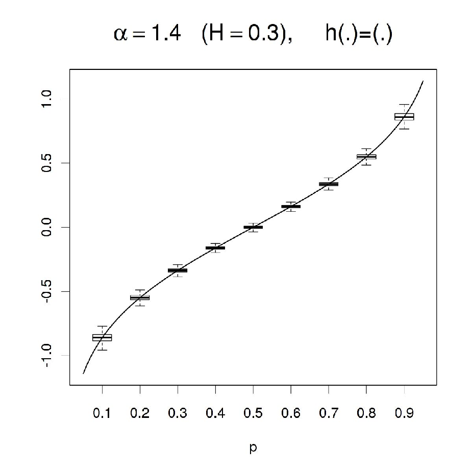
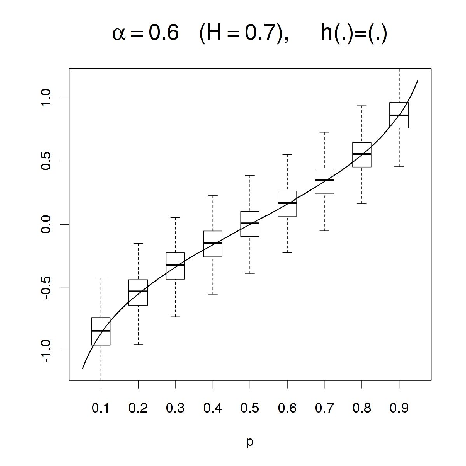
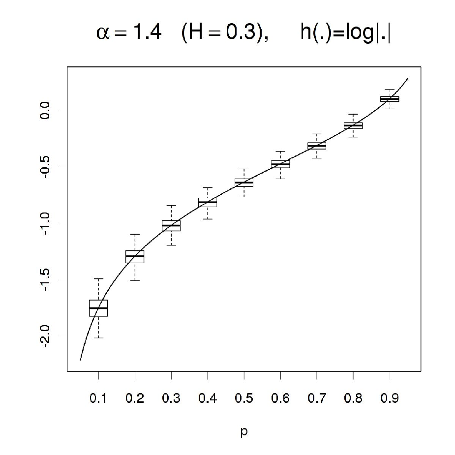
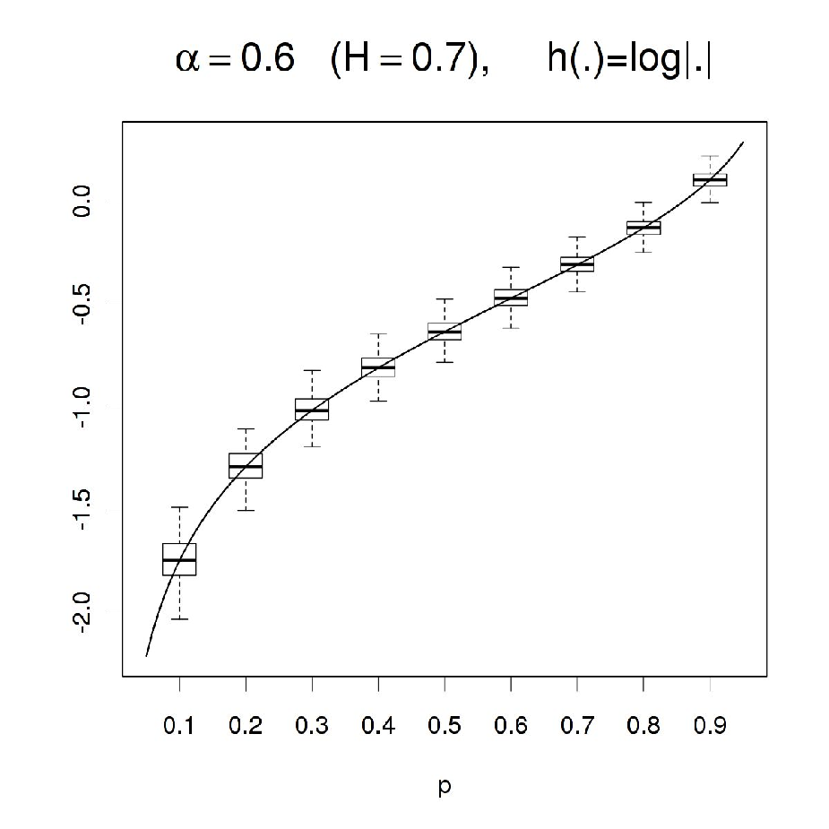
Figures 1 and 2 illustrate the convergence of the sample expectiles. Three $h$ functions are considered: $h(\cdot)=(\cdot)$, $(\cdot)^{2}$ and $\log|\cdot|$. The related Hermite rank of the function $\widetilde{\psi}$ is respectively 1,2 and 2 for these three $h$ functions. The sample size of the simulation is fixed to $n=500$. We can claim the convergence of the sample expectile $\widehat{E}(p;{h(Y)})$ towards $E_{h(Y)}(p)$ for all the values of $\alpha$ (or $H$), p and for the three functions $h$ considered. If we focus on $h(\cdot)=(\cdot)$, we can also remark a higher variance of the sample estimates for $\alpha=0.6$ compared to $\alpha=1.4$. This is in agreement with the theory since for $\alpha=0.6$, $\alpha\tau=0.6<1$ and the rate of convergence is lower than $n^{-1/2}$ which means an increasing of the variance. For the two other functions considered, then $\alpha\tau$ is always greater than 1 (it equals either 2.8 or 1.2 in our simulations) and we do not observe such an increasing of the variance.

To put emphasis on this last point, Figure 3 shows in log-scale the average (over the 9 order of expectiles considered in the simulation, i.e. $p=0.1,\ldots,0.9$) of the empirical variances in terms of $n$ for the three $h$ functions and for the two values of $\alpha=0.6$ and $\alpha=1.4$. We clearly observe that as soon as $\alpha\tau>1$, the slope of the curves is close to $-1$ which agrees with the result presented in Corollary 2 for example. When $h(\cdot)=1$ and $\alpha=0.6$, we observe that the slope is about $-0.6$ which seems to agree with the convergence in $n^{-\alpha\tau}$ which is expected from Theorem 1.

Let $\mathbf{X}=\left(X(i)\right)_{i=1,\ldots,n}$ be a discretized version of a fractional Brownian motion process and let $\mathbf{a}$ be a filter of length $\ell+1$ and of order $\nu\geq 1$ with real components i.e.:

$$\sum_{q=0}^{\ell}q^{j}a_{q}=0,\mbox{ for }j=0,\ldots,\nu-1\;\;\hskip 10.00002pt\mbox{ and }\hskip 10.00002pt\sum_{q=0}^{\ell}q^{\nu}a_{q}\neq 0.$$

Define also $\mathbf{X}^{\mathbf{a}}$ to be the series obtained by filtering $\mathbf{X}$ with $\mathbf{a}$, then:

$$X^{\mathbf{a}}\left(i\right)=\sum_{q=0}^{\ell}a_{q}X\left(i-q\right),\hskip 10.00002pt\mbox{ for }i\geq\ell+1$$

and $\mathbf{\tilde{X}}^{\mathbf{a}}$ as the normalized vector of $\mathbf{X}^{\mathbf{a}}$, i.e.:

$$\mathbf{\tilde{X}}^{\mathbf{a}}=\frac{\mathbf{X}^{\mathbf{a}}}{\mathbf{E}((X^{\mathbf{a}}(1))^{2})^{1/2}}.$$

It should be noticed here that the filtering operation allows to decorrelate the increments of the discretized version of the fractional Brownian motion process. Indeed, it may be proved (see e.g. Coeurjolly (2001)) that: $\rho_{H}^{a}(i)\sim k_{H}|i|^{2H-2\nu}$ as $|i|\rightarrow+\infty$.

Consider the sequence $(\mathbf{a}^{m})_{m\geq 1}$ defined by:

$$a_{i}^{m}\;=\left\{\begin{array}[]{ll}\ a_{j}&\;\mbox{if }i=jm\\ 0&\;\mbox{otherwise }\\ \end{array}\right.\hskip 20.00003pt\hskip 20.00003pt\mbox{for }i=0,\ldots,m\ell\;,$$

which is the filter $\mathbf{a}$ dilated $m$ times. It has been shown in Coeurjolly (2001); Coeurjolly (2008) that:

$$\tilde{\mathbf{X}}^{\mathbf{a^{m}}}=\frac{\mathbf{X}^{\mathbf{a^{m}}}}{\sigma_{m}}$$

where $\sigma_{m}^{2}=m^{2H}\sigma^{2}\kappa_{H}^{\mathbf{a}}$ and $\kappa_{H}^{\mathbf{a}}=\frac{-1}{2}\sum_{q,q^{\prime}=0}^{\ell}a_{q}a_{q^{\prime}}|q-q^{\prime}|^{2H}$.

The following proposition allows us to construct an ordinary least squares (OLS) estimator of the Hurst exponent $H$ of a fBm process based on sample expectiles.

We have:

	$\displaystyle\widehat{E}\left(p;{|\mathbf{X}^{\mathbf{a}^{m}}|^{\beta}}\right)$	$\displaystyle=$	$\displaystyle argmin_{\theta}{\frac{1}{n-m\ell}}\sum_{i=m\ell}^{n-1}|p-\mathbf{1}_{\{{|X^{\mathbf{a}^{m}}(i)|^{\beta}}\leq\theta\}}|.({|X^{\mathbf{a}^{m}}(i)|^{\beta}}-\theta)^{2}$
		$\displaystyle=$	$\displaystyle argmin_{\theta}{\frac{1}{n-ml}}\sum_{i=ml}^{n-1}|p-\mathbf{1}_{\{{|\tilde{X}^{\mathbf{a}^{m}}(i)|^{\beta}}\leq{\frac{\theta}{\sigma_{m}^{\beta}}}\}}|.({|\tilde{X}^{\mathbf{a}^{m}}(i)|^{\beta}}-\frac{\theta}{\sigma_{m}^{\beta}})^{2}.$

Setting $\theta^{\prime}=\frac{\theta}{\sigma_{m}^{\beta}}$, the proof of the first relation (9) follows easily. Using the same methodology, we can demonstrate the result given by equation (10).  

Now applying the logarithmic transformation to both sides of (9), we get:

$$\log\widehat{E}\left(p;{|\mathbf{X}^{\mathbf{a}^{m}}|^{\beta}}\right)=\beta H\log(m)+\log\left(\sigma^{\beta}(\kappa_{H}^{\mathbf{a}})^{\beta/2}E_{|Y|^{\beta}}(p)\right)+\log\left(\frac{\widehat{E}\left(p;{|\mathbf{\tilde{X}}^{\mathbf{a}^{m}}|^{\beta}}\right)}{E_{|Y|^{\beta}}(p)}\right).$$

(11)

On the other hand, (10) can be reformulated in the following way:

$$\widehat{E}\left(p;{\log|\mathbf{X}^{\mathbf{a}^{m}}|}\right)=H\log(m)+\frac{1}{2}\log(\sigma^{2}\kappa_{H}^{\mathbf{a}})+E_{\log|Y|}(p)+\left(\widehat{E}\left(p;{\log(|\mathbf{\tilde{X}}^{\mathbf{a}^{m}}|})\right)-{E_{\log|Y|}(p))}\right).$$

(12)

It is noteworthy here that we expect that $\log\widehat{E}\left(p;{|\mathbf{\tilde{X}}^{\mathbf{a}^{m}}|^{\beta}}\right)/E_{|Y|^{\beta}}(p)$ and $\widehat{E}\left(p;{\log(|\mathbf{\tilde{X}}^{\mathbf{a}^{m}}|^{\beta}})\right)-E_{\log|Y|}(p)$ to converge towards 0 as $n\rightarrow\infty$. Hence, based on equations (11) and (12), we opt for an OLS regression scheme. This allows to derive the two following estimators of the hurst index defined by:

$$\widehat{H}^{\beta}=\frac{{\mathbf{A}}^{\!T}}{\beta||\mathbf{A}||^{2}}\left(\log\widehat{E}\left(p;{|\mathbf{X}^{\mathbf{a}^{m}}|^{\beta}}\right)\right)_{m=1,\ldots,M},$$

(13)

and

$$\widehat{H}^{\log}=\frac{{\mathbf{A}}^{\!T}}{||\mathbf{A}||^{2}}\left(\widehat{E}\left(p;\log{|\mathbf{X}^{\mathbf{a}^{m}}|}\right)\right)_{m=1,\ldots,M},$$

(14)

where $\mathbf{A}$ is the vector of length $M$ with components $A_{m}=\log m-\frac{1}{M}\sum_{m=1}^{M}\log(m)$, $m=1,\ldots,M$ for some $M\geq 2$ whereas $||\mathbf{z}||$ for some vector $\mathbf{z}$ of length $d$ designates the norm defined by $\left(\sum_{i=1}^{d}z_{i}^{2}\right)^{1/2}$. Notice here that $\widehat{H}^{\beta}$ and $\widehat{H}^{\log}$ do not depend on $\sigma^{2}$.

We would like to put the stress on the fact that (13) and (14) are really similar to the ones developed in Coeurjolly (2001); Coeurjolly (2008). Indeed, the standard procedure developed in Coeurjolly (2001) simply consists in replacing the sample expectile by the sample variance (this method will be denoted by ST in Section 3.2). To deal with outliers, the procedure developed in Coeurjolly (2008) consists in replacing the sample expectile by either the sample median of $(\mathbf{X}^{\mathbf{a}^{m}})^{2}$ or the trimmed-means of $(\mathbf{X}^{\mathbf{a}^{m}})^{2}$. These two last methods are denoted by MED and TM in Section 3.2.

Now, we state the asymptotic results for these new estimates based on expectiles.

References

- Abry et al. (2000) P. Abry, P. Flandrin, M. S. Taqqu, and D. Veitch. Wavelets for the analysis, estimation, and synthesis of scaling data, pages 39–88. In Self-similar Network Traffic and Performance Evaluation. by K. Park and W. Willinger, Wiley, New York, 2000.
- Abry et al. (2003) P. Abry, P. Flandrin, M.S. Taqqu, and D. Veitch. Self-similarity and long-range dependence through the wavelet lens, pages 527–556. Theory and applications of long-range dependence. Birkhäuser, 2003.
- Achard and Coeurjolly (2010) S. Achard and J-F. Coeurjolly. Discrete variations of the fractional brownian motion in the presence of outliers and an additive noise. Statistics Surveys, 4:117–147, 2010.
- Arcones (1994) M.A. Arcones. Limit theorems for nonlinear functionals of stationary gaussian field of vectors. Ann. Probab., 22:2242–2274, 1994.
- Bardet et al. (2000) J.M. Bardet, G. Lang, E. Moulines, and P. Soulier. Wavelet estimator of long-range dependent processes. Statistical Inference for Stochastic Processes, 3:85–99, 2000.
- Beran (1994) J. Beran. Statistics for long memory processes. Monogr. Stat. Appl. Probab. 61. Chapman and Hall, London, 1994.
- Bijwaard and Franses (2009) G.E. Bijwaard and P. Hans Franses. The effect of rounding on payment efficiency. Computational statistics and data analysis, 53(4):1449–1461, 2009.
- Bois and Vignes (1982) P. Bois and J. Vignes. An algorithm for automatic round-off error analysis in discrete linear transforms. International Journal of Computer Mathematics, 12(2):161–171, 1982.
- Coeurjolly (2000) J.-F. Coeurjolly. Simulation and identification of the fractional brownian motion: a bibliographical and comparative study. J. Stat. Softw., 5(7):1–53, 2000.
- Coeurjolly (2001) J.-F. Coeurjolly. Estimating the parameters of a fractional brownian motion by discrete variations of its sample paths. Stat. Infer. Stoch. Process., 4(2):199–227, 2001.
- Coeurjolly (2008) J.-F. Coeurjolly. Hurst exponent estimation of locally self-similar gaussian processes using sample quantiles. Annals of Statistics, 36(3):1404–1434, 2008.
- Daubechies (1992) I. Daubechies. Ten lectures on wavelets. CBMS-NSF Regional Conference Series on Applied Mathematics, 61. SIAM, Philadelphia, 1992.
- Faÿ et al. (2009) G. Faÿ, E. Moulines, F. Roueff, and M.S. Taqqu. Estimators of long-memory: Fourier versus wavelets. Journal of econometrics, 151(2):159–177, 2009.
- Flandrin (1992) P. Flandrin. Wavelet analysis and synthesis of fractional brownian motion. IEEE Trans. Inform. Theory., 38(2, part 2):910–917, 1992.
- Ghosh (1971) J.K. Ghosh. A new proof of the bahadur representation of quantiles and an application. The Annals of Mathematical Statistics, 42(6):1957–1961, 1971.
- Hampel et al. (1986) F. R. Hampel, E. M. Ronchetti, P. J. Rousseeuw, and W. A. Stahel. Robust Statistics: The Approach Based on Influence Functions. Wiley, New York, 1986.
- Huber (1981) P. J. Huber. Robust statitics. Wiley series in probability and mathematical statistics. Wiley, 1981.
- Istas and Lang (1997) J. Istas and G. Lang. Quadratic variations and estimation of the holder index of a gaussian process. Ann. Inst. H. Poincaré Probab. Statist., 33:407–436, 1997.
- Kent and Wood (1997) J.T. Kent and A.T.A. Wood. Estimating the fractal dimension of a locally self-similar gaussian process using increments. J. Roy. Statist. Soc. Ser. B, 59:679–700, 1997.
- Kouamo et al. (2010) O. Kouamo, C. Lévy-Leduc, and E. Moulines. Central limit theorem for the robust log-regression wavelet estimation of the memory parameter in the gaussian semi-parametric context, 2010. arXiv:1011.4370.
- Mandelbrot and Ness (1968) B. B. Mandelbrot and J. W. Van Ness. Siam review. IEEE Transactions on Pattern Analysis and Machine Intelligence, 10:422–437, 1968.
- Matthieu (2006) M. Matthieu. Semantics of roundoff error propagation in finite precision calculations. Higher-order and symbolic computation, 19(1):7–30, 2006.
- Newey and Powell (1987) W.K. Newey and J.L. Powell. Asymmetric least squares estimation and testing. Econometrica, 55:819–847, 1987.
- Percival and Walden (2000) D. B. Percival and A. T. Walden. Wavelet Methods for Time Series Analysis. Cambridge University Press, 2000.
- Robinson (1995) P. Robinson. Gaussian semiparametric estimation of long range dependence. Ann. Stat., 23:1630–1661, 1995.
- Rosenbaum (2009) M. Rosenbaum. Integrated volatility and round-off error. Bernoulli, 15(3):687–720, 2009.
- Soltani et al. (2004) S. Soltani, P. Simard, and D. Boichu. Estimation of the self-similarity parameter using the wavelet transform. Signal Process., 84:117–123, 2004.
- Taqqu (1977) M.S. Taqqu. Law of the iterated logarithm for sums of non-linear functions of gaussian variables that exhibit a long range dependence. Z. Wahrscheinlichkeitstheorie verw. Geb., 40:203–238, 1977.
- Vilmart (2008) G. Vilmart. Reducing round-off errors in rigid body dynamics. Journal of Computational Physics, 227(15):7083–7088, 2008.
- Williams (2006) E. Williams. The effects of rounding on the consumer price index. Monthly labor review, 129(10):80–89, 2006.
- Wood and Chan (1994) A.T.A. Wood and G. Chan. Simulation of stationary gaussian processes in . J. Comput. Graph. Statist., 3:409–432, 1994.
- Wornell and Oppenheim (1992) G. Wornell and A. Oppenheim. Estimation of fractal signals from noise measurements using wavelets. IEEE Transactions on Signal Processing, 40:611–623, 1992.