Expansion dynamics of the Fulde-Ferrell-Larkin-Ovchinnikov (FFLO) state
Abstract
We consider a two-component Fermi gas in presence of spin imbalance, modelling the system in terms of a one-dimensional (1D) attractive Hubbard Hamiltonian initially in presence of a confining trap potential. With the aid of the time-evolving block decimation (TEBD) method, we investigate the dynamics of the initial state when the trap is switched off. We show that the dynamics of a gas initially in the FFLO state is decomposed into the independent expansion of two fluids, namely the pairs and the unpaired particles. In particular, the expansion velocity of the unpaired cloud is shown to be directly related to the FFLO momentum. This provides an unambiguous signature of the FFLO state in a remarkably simple way.
Ultracold gases have provided experimental verification for several fundamental concepts of quantum physics. The direct access to momentum distribution and correlations via time-of-flight expansion has played a key role in many landmark experiments. Mapping of momentum to position after time-of-flight revealed Bose-Einstein condensation [1]. Coherence manifesting after expansion gave evidence of the phase of the condensate [2], and of the superfluid - Mott insulator transition [3]. Inversion of the aspect ratio of an expanding Fermi gas revealed hydrodynamic behaviour [4, 5]. A major goal is to observe the elusive Fulde-Ferrel-Larkin-Ovchinnikov (FFLO) state which is at the heart of understanding the interplay between superconductivity and magnetism. While experiments in solid state systems [6, 7, 8] and ultracold gases [9] are consistent with the state, an unambiguous observation is lacking.
The FFLO phase is characterized by the formation of pairs with nonzero overall momentum [10, 11]. This property manifests itself through the appearance of an oscillating (superconducting) order parameter , where is the so-called FFLO momentum () [12]. It is given by the mismatch between the Fermi momenta of spin up and spin down particles: . In contrast, zero-momentum () pairs give the conventional BCS superconductor physics. Despite the lack of genuine long range order, the FFLO state has been theoretically predicted to be especially stable in one-dimensional systems [13, 14, 15], as well as in quasi-1D [16, 17, 18]. Inspired by the first experiments in imbalanced atomic Fermi gases [19, 20], various methods for detecting the FFLO state in ultracold gases have been proposed (see [21] and references therein). In this letter we show via exact simulations that time-of-flight expansion provides a smoking gun signature of the FFLO state in one dimension, see Figure 1. Expansion and consequent imaging of densities is a widely used basic technique in experiments with ultracold gases.

The characteristic parameters can be chosen so that the lattice model employed is a good approximation for a continuum model of a spin-imbalanced gas in 1D in the strong interaction limit [16, 22, 23]. With appropriate mapping of the parameters, in the strong interaction limit, our predictions are thus relevant for experiments in 1D potentials as in [9].
We consider the 1D Fermi-Hubbard Hamiltonian in presence of an overall confining potential
| (1) |
where () creates (annihilates) a spin particle at the lattice site , is the hopping constant, is the interaction strength between the two species, and the strength of the trapping potential. For a harmonic potential , where denotes the trap center, and for a box potential is specified below.
To obtain the ground state and time evolution of the system, we have employed the (essentially) exact time-evolving block decimation (TEBD) algorithm [24] with Schmidt number and simulation timestep . As results from TEBD we obtain the single particle densities , , the doublon density , and the ground state pair correlation and its momentum transform , which are given by
| (2) |
| (3) |
where describes the quantum mechanical average over the state , and are lattice site indices, is the imaginary unit and is the size of the lattice.
We have experimented within TEBD paramater ranges , , , , , and , where is the polarization and is the harmonic trapping strength. Many simulations were performed also using a box potential. Single runs with the larger parameters have been done in order to check that the qualitative description of the dynamics stays the same when changing the parameters. Indeed, the important characteristics of the dynamics are the same in all of the scenarios.
For simplicity we first consider here the box trap. In Figure 2 we show results for 10 up-particles and 6 down-particles, with . The ground state is a 1D FFLO state, characterized by a peak in the pair momentum distribution that coincides with the definition of the FFLO momentum . Figure 2 shows the ground state density profile in which the small oscillations characterize the FFLO state. However, such delicate features are hard to resolve in ultracold gas experiments, and therefore other signatures are needed. Figure 2 displays the pair momentum correlation function.


The dynamics after releasing the particles from the potential show a striking two-fluid behaviour. Pairs (doublons) and excess unpaired majority particles expand as effectively non-interacting fluids, as can be seen from Figure 3.


Indeed, we have compared the dynamics with strong interaction between the spins to the dynamics of non-interacting particles and verified that the doublons and unpaired particles in the strongly interacting limit expand qualitatively just like non-interacting particles would (see supplementary information Figures 2-5 for the results [25]). The important difference is, however, that the velocity of the expansion is changed with respect to the non-interacting case. The doublons expand with velocities up to . And what is crucial for our proposal for observing the FFLO state: the unpaired particles expand with velocities up to , where is the FFLO momentum. In the case shown here the unpaired particle velocity is larger than the pair one, but in general the relative velocities of pairs vs. unpaired particles is not essential for the method since the up and down components can be imaged separately, see e.g. [9].
A wavefront corresponding to clearly separates from the rest of the unpaired particle cloud during initial dynamics (), after which it moves with a constant velocity at the edge of the cloud, see Fig.3. Therefore, by measuring the expansion velocity of the cloud edge (), e.g. from the maximum gradient of the density (see supplementary information Figure 1 [25]), one obtains the FFLO momentum from
| (4) |
The momentum obtained in this way from our simulations is compared in Figure 4 to the FFLO momentum as given by the definition (and by the peak in the momentum pair correlation function of the ground state, c.f. Figure 2). For reference, we show the expansion velocities in the cases of a non-interacting gas, and a non-FFLO state without pair coherence (discussed later in the text). Only in the case of the FFLO state does the expansion velocity depend on the imbalance. The extracted from the simulations via Eq.(4) matches excellently the expected FFLO momentum.
In the experimentally relevant case of a harmonic trap, can be determined in the same way as discussed above. Figure 4 shows the comparison of obtained from the edge expansion velocity to the FFLO momentum in a harmonic trap. The time evolution is shown in Figure 5. In , the Fermi momenta are the highest momenta in the harmonic oscillator eigenstates of the quantum numbers and , respectively (see supplementary information [25]). In the limit of a shallow trap and large particle number, one approaches the box potential case and a local density approximation (LDA) argument can be used for the extraction of [26].


The interpretation of our numerical results in terms of the expansion of two fluids is supported by a rigorous Bethe-ansatz analysis of the one-dimensional Fermi-Hubbard Hamiltonian [27, 23, 22]. In the strong-coupling limit, the system can be described as two weakly interacting spinless Fermi gases, corresponding to pairs and unpaired particles whose maximum group velocities are the respective Fermi velocities. We thus expect the time evolution of the system to be approximately generated by the free-particle Hamiltonians for unpaired particles and pairs. In the case of a lattice model, the group velocity for each momentum component is , where the constant depends on the nature of the particle considered. In our pair/unpaired particle 2-fluid model stemming from the Hubbard Hamiltonian, we have for the unpaired particles and for the pairs. For , the relation thus allows to establish a connection between the maximal expansion velocity and the Fermi momentum of each component (note that for the maximal expansion velocity is given by ).
Based on our numerical findings, we now assume that the unpaired-particle Fermi momentum and the FFLO momentum share the same value . This is supported by Bethe-ansatz analysis in the continuum case [28] and is also intuitive: in the limit of strong interactions the pair kinetic energies are small and it is energetically favourable that the ground state structure allows the lowest momentum states up to to be mainly occupied by unpaired majority particles. Thus measuring the maximal expansion velocity of the unpaired particles gives access to the value of the FFLO momentum. As seen in Figure 4, this scenario agrees with the numerical results, providing a clear signature of the FFLO state. The lattice reproduces the continuum-case dynamics for low densities [16, 22] (we have tested also the low density limit), and our proposal is thus expected to be suitable for the detection of the FFLO state in experiments of the type [9]. Moreover, the proposed method should be robust with respect to averaging over an array of 1D tubes, c.f. [9].
Our simulations describe the zero temperature case. Quantum Monte Carlo calculations suggest that there is a finite-temperature precursor for the FFLO state which involves pairing but no FFLO-type correlations [29]. Is the signature we propose for the FFLO state distinguishable from any traces of a state with pairing but no FFLO correlations? Simulating exact dynamics at finite temperature is a formidable task and well beyond the state-of-the-art. However, to consider pairing without FFLO correlations, we have simulated the dynamics of various initial states which have the same average densities of unpaired and paired particles as the corresponding FFLO states, but which possess no correlations between the particles or between the pairs. Such an uncorrelated state can be written as an ensemble of product states, in which each of the product states have completely spatially localized pairs and single majority particles. Choosing the constituents of the ensemble randomly and giving them equal weight, we obtain the results shown in Figure 4: the expansion velocity does not depend on the polarization. It is simply given by and for unpaired particles and pairs, respectively. Therefore, observing a change of the unpaired particle expansion velocity with the polarization, such that it has the functional dependence , is a genuine signature of the FFLO correlations, and cannot be achieved for a non-correlated, paired state with the same imbalance. When lowering the temperature, emergence of a -dependent expansion front on top of a thermal state background would reveal that the FFLO state has been reached.
To conclude, we have shown that like in many classic ultracold gas experiments, also in the case of the long-sought-for FFLO state, the expansion of the cloud gives an exceedingly simple way of determining the nature of the initial state. Our exact quantum many-body simulations of the 1D imbalanced gas present a clear two-fluid behaviour with characteristic expansion velocities. We show that the matching of the expansion velocity of the unpaired majority cloud with the expected FFLO momentum provides an unambiguous signature of the FFLO state.
Acknowledgements: We thank R.G. Hulet for useful discussions. This work was supported by the Academy of Finland (Projects 213362, 217043, 217045, 210953, 135000, and 141039), ERC (Grant No. 240362-Heattronics), and conducted as a part of a EURYI scheme grant (see www.esf.org/euryi). Computing resources were provided by CSC - the Finnish IT Centre for Science.
References
- [1] M. H. Anderson, et al., Science 269, 198 (1995).
- [2] M. R. Andrews, et al., Science 275, 637 (1997).
- [3] M. Greiner, et al., Nature 415, 39 (2002).
- [4] K. O’Hara, et al., Science 298, 2179 (2002).
- [5] C. Menotti, P. Pedri, and S. Stringari, Phys. Rev. Lett. 89, 250402 (2002).
- [6] H. A. Radovan, et al., Nature 425, 51 (2003).
- [7] A. Bianchi, R. Movshovich, C. Capan, P. G. Pagliuso, J. L. Sarrao, Phys. Rev. Lett. 91, 187004 (2003).
- [8] R. Casalbuoni and G. Nardulli, Rev. Mod. Phys. 76, 263 (2004).
- [9] Y.-A. Liao, et al., Nature 467, 567 (2010).
- [10] P. Fulde and R. A. Ferrell, Phys. Rev. 135, A550 (1964).
- [11] A. I. Larkin and Y. N. Ovchinnikov, Zh. Eksp. Teor. Fiz. 47, 1136 (1964).
- [12] S. Takada and T. Izuyama, Prog. Theor. Phys. 41, 635 (1969).
- [13] A. E. Feiguin and F. Heidrich-Meisner, Phys. Rev. B 76, 220508 (2007).
- [14] G. G. Batrouni, M. H. Huntley, V. G. Rousseau, R. T. Scalettar, Phys. Rev. Lett. 100, 116405 (2008).
- [15] M. Rizzi, et al., Phys. Rev. B 77, 245105 (2008).
- [16] K. Yang, Phys. Rev. B 63, 140511 (2001).
- [17] G. Orso, Phys. Rev. Lett. 98, 070402 (2007).
- [18] M. M. Parish, S. K. Baur, E. J. Mueller, D. A. Huse, Phys. Rev. Lett. 99, 250403 (2007).
- [19] M. W. Zwierlein, et al., Science 311, 492 (2006).
- [20] G. B. Partridge, et al., Science 311, 503 (2006).
- [21] M. R. Bakhtiari, M. J. Leskinen, and P. Törmä, Phys. Rev. Lett. 101, 120404 (2008); A. Korolyuk, F. Massel, and P. Törmä, Phys. Rev. Lett. 104, 236402 (2010); J. M. Edge, N. R. Cooper, Phys. Rev. A 81, 063606 (2010); M. Swanson, Y. L. Loh, and N. Trivedi, arXiv: 1106.3908v1 (2011).
- [22] E. Zhao and W. V. Liu, Phys. Rev. A 78, 063605 (2008).
- [23] E.H. Lieb, and F.Y. Wu, Phys. Rev. Lett. 20, 1445 (1968); F. H. L. Essler, et al., The One-Dimensional Hubbard Model (Cambridge University Press, 2005).
- [24] A. J. Daley, et al., J Stat Mech-Theory E p. P04005 (2004).
- [25] J. Kajala, F. Massel, and P. Törmä, Supplementary information.
- [26] M. Tezuka and M. Ueda, Phys. Rev. Lett. 100, 110403 (2008).
- [27] T. Giamarchi, Quantum Physics in One Dimension (International Series of Monographs on Physics) (Oxford University Press, USA, 2004).
- [28] N. Oelkers, et al., J Phys A-Math Gen 39, 1073 (2006).
- [29] M. Wolak, et al., Phys. Rev. A 82, 013614 (2010).
I Supplementary Material
II Dynamics of the Gaudin-Yang model in the strongly attractive regime
As shown in [1], the Bethe-ansatz solution for the Gaudin-Yang model in the strongly interacting regime can be written in terms of the quasi-momenta ( for unpaired particles, for pairs) and the spin roots
| (5) | |||||
| (6) | |||||
| (7) | |||||
where represents the size of the system and the contact interaction strength, while and are constants related to and . Note that has been rescaled so that the physical value of the interaction strength is given by . Eqs. (5-7) allow us to rewrite the dispersion relation for the system
| (8) |
in the following form
| (9) |
From Eq. (9), we recognize the pair contribution to the kinetic energy (), along with the pair-binding energy () and the single-particle kinetic energy (). We can thus state that since, in the strongly interacting limit, the binding energy depends on the interaction energy only, it is independent of the Fermi energy. Remembering the definition of , for large interaction (i.e. ), it is possible to rewrite the pair kinetic energy term as
| (10) |
with . The term can be identified with the quasi momentum of a free particle in a system of size . If we calculate the velocity of such object
| (11) |
we can conclude that, in the strong-coupling limit, along with excitations with group velocity (particles), excitations moving with group velocity are present. We identify these excitations with pairs with binding energy and mass .
III Uncorrelated State Dynamics
The uncorrelated state dynamics originates from the dynamics of localized particles released into the lattice, similiar to the case previously studied in [2]. The expansion wavefronts which emerge have velocities and , which is in accordance with our understanding that we see the maximum velocities of unpaired particles and pairs in the dynamics. Note that localization to a lattice site corresponds in the Fourier space to employing all momenta in the band. The maximum expansion velocities observed correspond to momenta since, due to the lattice dispersion , , where we have for unpaired particles and for pairs.
IV Determining the edge expansion velocity
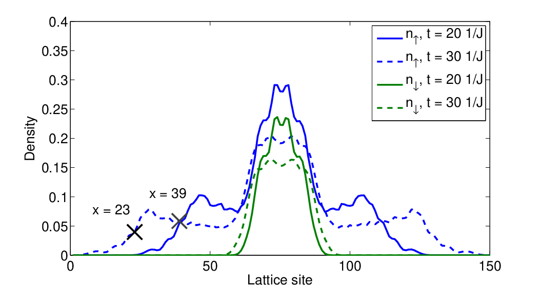
The edge expansion velocity has been determined using the numerically obtained density profiles at different times after the release from the trapping potential. We are interested in the maximum group velocity of the unpaired component, as this gives the FFLO momentum . In the simulations it is seen that this unpaired wavefront separates from the rest after initial dynamics () after which it travels at constant velocity at the edge of the cloud. The velocity of the edge wavefront has been determined by calculating the change of the position of the maximum gradient of the unpaired majority particle density at the edge. Figure 6 illustrates how this has been done.
V Comparing non-interacting and strongly interacting expansion dynamics
Figures 7 - 10 illustrate how the expansion profiles of X doublons and Y unpaired particles look qualitatively like the expansion profiles of X and Y non-interacting particles, respectively, but have different velocities compared to the non-interacting case. The velocity in the strongly interacting regime is for the unpaired particles and for the pairs (down is the minority species). In the noninteracting case, the expansion velocity of species is given by .
VI Additional data
Figure 11 depicts the ground state of the 1D FFLO superfluid in a harmonic trap as described in the main text. The density is low enough so that the lattice result corresponds to the continuum case in the strongly interacting regime. Corresponding to this ground state, Figure 12 shows the momenta involved in FFLO pairing in the case of a harmonic trap with small particle number.
Looking at Figure 12, the determined from the expansion velocity matches which has been calculated from noninteracting quantum harmonic oscillator eigenstates. To elaborate, for example for five particles has been obtained from the peak at maximum momentum in the momentum distribution of the 5th quantum harmonic oscillator eigenstate (i.e. , since the harmonic oscillator quantum numbers start from ). Moreover, the pair momentum correlator matches calculated again using the noninteracting harmonic oscillator eigenstates ( for the 1st eigenstate which is a Gaussian centered at zero). The quantity corresponds to pairing between a down particle at the lowest level () and an up particle at the level , whereas corresponds to a pairing between a down particle at and an up particle at . For larger particle numbers the peak of and (and thus as obtained from the expansion velocity) converge into the same value, as verified by our numerical simulatons with larger particle numbers (see Figure 14). In comparison, for the box potential, the peak of , and as obtained from the expansion velocity are alread the same for small particle numbers due to the box eigenstates being momentum eigenstates (see Figure 13). For larger particle numbers, the box potential becomes a reasonable approximation for the harmonic potential, and thus the values of the peak of , and as obtained from the expansion velocity become the same. This explains why the local density approximation works also in a harmonic trap for determining the FFLO momentum using for large particle numbers.



References
- [1] N. Oelkers, et al., J Phys A-Math Gen 39, 1073 (2006).
- [2] J. Kajala, F. Massel, and P. Törmä, Phys. Rev. Lett. 106, 206401 (2011).