KCL-MTH-11-12
Moduli space coordinates and excited state -functions
G.M.T. Watts **
*
Email: gerard.watts@kcl.ac.uk
Department of Mathematics, King’s College London,
Strand, London WC2R 2LS – UK
Abstract
We consider the space of boundary conditions of Virasoro minimal models formed from the composition of a collection of flows generated by between conformal boundary conditions. These have recently been shown to fall naturally into a sequence, each term having a coordinate on it in terms of a boundary parameter, but no global parameter has been proposed. Here we investigate the idea that has been put forward that the overlaps of particular bulk states with the boundary states give natural coordinates on the moduli space of boundary conditions. We find formulae for these overlaps using the known thermodynamic Bethe Ansatz descriptions of the ground and first excited state on the cylinder and show that they give a global coordinate on the space of boundary conditions, showing it is smooth and compact as expected.
1 Introduction
The space of boundary conditions for Virasoro minimal models have been investigated quite extensively. Distinguished amongst these boundary conditions are the conformal boundary conditions which have been classified by Cardy [1] and Petkova et al. [2]. These can be connected by renormalisation group flows generated by relevant boundary fields. A special class of these are the integrable boundary flows generated by the field . These flows were first considered by Recknagel et al [5]. They can be joined into a sequence which appeared in [6]11 1 It should be noted that the actual equations for the g-functions of the bulk off-critical flows in this paper are not correct, but exactly at the bulk critical point they do correctly reproduce the sequence of boundary flows and has arisen naturally in recent work by Gaberdiel et al. [7] and Dorey et al. [4]. In [7], the flows fall into separate pieces which then have to be joined together by hand to form the whole sequence; in [6, 4] there is a separate parameter which can take the bulk theory slightly off-critical in which case the whole sequence of boundary flows arises with a single parameter, but as the bulk theory becomes critical (conformal) the boundary flows again break into disjoint sets. Finally, the same sequence arises when the truncated conformal space approach is used to study boundary flows [8]; again this sequence disappears as the truncation level regulator is removed.
In this paper we investigate the idea suggested in [11] that the overlaps of bulk states with boundary states could provide useful coordinates on the space of boundary conditions. The basic such overlap is the ground state overlap which is also called the g-function or ground state entropy. For purely elastic scattering theories, there are general formulae for mixed bulk–boundary flows [12, 13] which reduce to those in [14] for purely boundary flows (The results in [14] are not correct when there is a simultaneous bulk perturbation). The minimal models have been investigated in [4] using a relationship with the purely-elastic staircase model but at present general results for kink models are not known.
We start with a consideration of the tri-critical Ising model (TCIM for short). In the approximate mean-field approach [9], the natural coordinate to take on the space of boundary conditions is the magnetisation at the boundary. In the conformal case the bulk spin field diverges as it approaches the boundary but we can consider a similar quantity, the expectation of the bulk spin field on a disk. The bulk spin field in the TCIM is [10] and the expectation value on a disk is the ratio of the overlaps of the states and with the boundary state.
The g-functions along the TCIM boundary flows were derived by Nepomechie and Ahn in [15]22 2 The g-functions derived in [15] are only correct for the purely boundary flows; when bulk perturbations are included they suffer from the same problems described in [11] as well as being implicitly defined in [25]. Nepomechie and Ahn did not consider the excited state g-functions corresponding to the state , but we can take the bulk TBA equations for this state proposed in [16, 17] and put them into the formulae of [15] we do indeed obtain functions which correctly interpolate the overlap of with the conformal boundary state; these are our proposals for the excited state g-functions in this case.
The paper is organised as follows. In section 2 we summarise the known facts about the tri-critical Ising model, its boundary conditions and related TBA systems. In section 3.3 we present our proposals for the excited state TBA g-functions and show that provides a good coordinate on the space of boundary conditions. In section 4 we present the generalisation to an arbitrary diagonal unitary minimal model.
2 The boundary tri-critical Ising model
The space of boundary conditions and their interpolating flows in the TCIM was first presented by Affleck in [18] and includes the following
| (2.1) |
where the boundary conditions are labelled according to their interpretation in terms of the allowed values of a lattice spin taking values in ; Each flow is generated by a field of conformal weight . The boundary conditions can also be labelled by their Kac labels [19]: there are three fixed boundary conditions and two variable boundary conditions and . The final elementary boundary state is not part of this sequence.
We would like to give a parametrisation of the whole space (2.1) – it appears to be an entirely natural sequence of flows which form a one-dimensional subspace of the space of boundary conditions and if the space of boundary conditions is a genuine moduli space one ought to be able to put coordinates on it.
In terms of a mean-field approximation [9], the space (2.1) can be parametrised by the value of the boundary magnetisation, . This takes values and in particular
| (2.2) |
In the conformal field theory, the spin field is represented by the conformal field of conformal weight [10]. This field diverges as it approaches any of the conformal boundary conditions apart from and so it does not have a finite boundary magnetisation.
We can choose instead a related quantity, , the expectation value of the bulk spin on a unit disk with the appropriate boundary condition. This is directly related to the divergence of the spin as it approaches the boundary, being just the bulk-boundary structure constant.
If we restrict for now to the case of a conformal boundary condition , we can define the boundary state
| (2.3) |
where are the Ishibashi states for the representation The coefficient is the g-function introduced in [20]. The structure constant appears in the bulk-boundary operator product expansion of a bulk field approaching a conformal boundary condition at
| (2.4) |
This allows one to calculate the partition function on the unit disk with the insertion of in two ways as
| (2.5) |
so that can be found as the expectation value of the bulk field,
| (2.6) |
For the diagonal unitary minimal models, where is the modular S–matrix [1]. The numerical values of the and some useful combinations are in table 1.
We would like to take as the coordinate along the space of flows (2.1). As can be seen in table 1, this increases along the fixed points of the flow (2.1) and we expect this will remain true for all the flow, not just the fixed points, but to check that we need to find a way to calculate it at non-critical points. To do that we will use TBA methods which are explained in the next section.
3 The TBA description of the tri-critical Ising model
We want to find equations for when is a perturbed boundary condition. The standard -function can be found by integrating suitable functions from the bulk TBA system against kernels determined by the boundary reflection matrices; is an “excited -function” or an overlap of the boundary state with an excited state which is expected to be given by integrating excited state TBA functions against the same kernels. In the case of the Yang-Lee model the first excited state can be found by analytic continuation of the ground state in the perturbation parameter [22] and so the excited state g-functions can also be found that way. For the TCIM, the first excited state is in a different sector of the model (it is odd under the symmetry rather than even like the ground state) so it is very unlikely to be simple to connect it to the ground state, but there are related TBA-like equations which describe it, as proposed in [17].
The TBA equations for the ground state come in three varieties: the massless TBA for the model given by the addition of the bulk field with a positive coupling which flows to the critical Ising model [21]; the massive TBA for the model given by the addition of the bulk field with a negative coupling which flows to a model with one massive kink [23]; the kink TBA which describes the purely critical model and can be found as the common limit of the massive and massless TBA systems. We shall restrict ourselves to the kink system which is all we need to describe the boundary flows in the critical bulk model.
3.1 The kink TBA equations for the ground state
The kink TBA equations for the ground state are integral equations for two functions ,
| (3.1) |
where , and is an essentially irrelevant parameter. The ground state energy is given in terms of this system by
| (3.2) |
The four separate flows in the sequence (2.1) can each be labelled by a parameter for which the UV is given by and the IR by , and the g-functions are given as [15, 25]
| (3.3) | |||||
| (3.4) |
3.2 The kink TBA equations for the first excited state
The TBA equations proposed in [17] for the first excited state of conformal weight are the very similar set
| (3.5) |
where . The energy of is given in terms of this system as
| (3.6) |
If we substitute for in equations (3.3) and (3.4) we find we have constructed the TBA formulae for the perturbed excited state g-functions:
| (3.7) | |||||
| (3.8) |
and consequently we have formulae for the one-point function of the spin field along the flows in terms of the solutions of the ground state and excited state TBA equations:
| (3.9) | |||||
| (3.10) |
The g-functions and b-functions for the remaining two flows and are found from these by the spin-reversal symmetry.
3.3 Results for the tri-critical Ising model
The TBA equations (3.1) and (3.5) are easy to solve by discretisation and iteration. In figure 1(a) we plot the functions and in figure 1(b) we plot , where the convolution is . These can be seen to interpolate the UV values for large negative and the IR values for large positive .


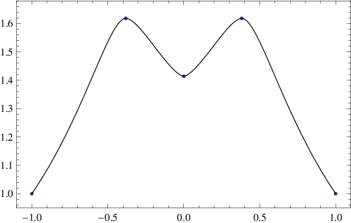
It is also very helpful to plot the sequence of flows (2.1) in with coordinates and which we do in figure 2. This shows that provide a good global coordinate along the sequence of flows, as well as highlighting the fixed points which are the stationary points of .
4 The general minimal model moduli space
We now propose the extension of the result in section 2 to the general unitary minimal model . The minimal model can be formulated in terms of a single spin taking values in – this can be thought of as the average value of the spins at each end of an edge in the standard RSOS realisation. The spin field in the Landau-Ginzburg description [24] related to the lattice realisation is again . There is a similar basic sequence of boundary flows generated by the boundary field : given in terms of Kac labels, this is
| (4.1) |
The boundary states correspond to fixed boundary spins and the boundary states correspond to spins which can take two consecutive values.
4.1 The case of even:
For the case of even, the ground state TBA equations are given in [23] and the excited state TBA equations for the state are again given in [17]. The -functions can be found in [25] in terms of the eigenvalues of certain operators which are simply related to the ground-state TBA functions; they are simple generalisation of those for the tri-critical Ising model. The ground state kink TBA is a system of integral equations for functions :
| (4.2) |
where is the incidence matrix of the Dynkin diagram. The first excited state kink TBA of [17] is the related set
| (4.3) |
where and the sign for and otherwise. From [25] we find that the g-functions for the flows in (4.1) with are given by
| (4.4) |
and we propose that the excited state g-functions are given by the replacement of the ground state TBA functions in these expressions by the excited state functions:
| (4.5) |
Using these, in figure 3 we plot vs for the models with and .

As can be seen, the functions we propose interpolate the conformal fixed points as required, the fixed boundary conditions are local minima of the g-function and the boundary conditions are local maxima.
4.2 The case of odd:
The odd minimal models are slightly different. The ground state TBA equations are given in [23] and the kink ground state equations are exactly as in (4.2) but the first excited state TBA equations do not appear to have been written down so far. We propose that the kink TBA equations for the case of a critical bulk are also exactly as in (4.3), with the same assignment of signs. This is asymmetric, for example the signs for are nevertheless they appear to be correct. The boundary state overlaps are also slightly more complicated having logarithmic terms and cannot be directly deduced from the TBA equations using the results of [25]. We propose that they are also given by (4.4) and (4.5); these pass several perturbative and non-perturbative tests which we plane to report on at greater length elsewhere. We include plots of and for and in figure 3.
5 Conclusions
We have a global coordinate on a space of boundary flows in the unitary minimal models in terms of two sets of TBA equations. This answers the question put in [8], whether such a unified coordinate can be found. It shows that the space of flows is indeed compact and smooth. It would be very interesting to see if the same quantities can be calculated in the staircase model which was used in [6] and [4] to study the simple g-function.
Finally we remark that, as has been noted before, the values of
and for the
boundary condition in
the model are the same as those for the boundary condition
for the model (provided ). This can be
explained by the fact that the corresponding conformal defects are
essentially the same operator – something we hope to return to later.
Acknowledgements
I would like to thank P. Giokas and P.E. Dorey for very helpful discussions and STFC grant ST/G000395/1 for support. All numerical work was performed using Mathematica [26].
References
- [1] J.L. Cardy, Boundary conditions, fusion rules and the Verlinde formula, Nucl. Phys. B 324 (1989) 581
- [2] R.E. Behrend, P.A.Pearce, V.B. Petkova and J.-B. Zuber, Boundary conditions in rational conformal field theories, Nucl. Phys. B 570 (2000) 525–589 [hep-th/9908036]
- [3] P.E. Dorey, C. Rim and R. Tateo, Exact g-function flow between conformal field theories, Nucl. Phys. B 834 (2010) 485–501 [arXiv:0911.114969]
- [4] P.E. Dorey, R. Tateo and R. Wilbourne, Exact g-function flows from the staircase model, Nucl. Phys. B 843 (2011) 724–752 [arXiv:1008.1190]
- [5] A. Recknagel, D. Recknagel and V. Schomerus, On relevant boundary perturbations of unitary minimal models, Nucl. Phys. B 588 (2000) 552–564 [hep-th/0003110]
- [6] F. Lesage, H. Saleur and P. Simonetti, Boundary flows in minimal models, Phys. Lett. B427 (1998) 85–92 [hep-th/9802061]
- [7] S. Fredenhagen, M.R. Gaberdiel and C. Schmidt-Colinet, Bulk flows in Virasoro minimal models with boundaries, J. Phys. A42 (2009) 495403 [arXiv:0907.2560]
- [8] G.M.T. Watts, On the renormalisation group for the boundary truncated conformal space approach [arXiv:1104.0225]
- [9] P. Giokas, Mean field theory for boundary Ising and tri-critical Ising models, arXiv:1106.1843
- [10] M. Lässig, G. Mussardo and J.L. Cardy, The scaling region of the tricritical Ising model in two dimensions , Nucl. Phys. B 348 (1991) 591-618.
- [11] P.E. Dorey. I Runkel, R. Tateo and G.M.T. Watts, g-function flow in perturbed conformal field theory, Nucl. Phys. B 578 (2000) 85-122 [hep-th/9909216]
- [12] P.E. Dorey, D. Fioravanti, C. Rim and R. Tateo, Integrable quantum field theories with boundaries: the exact g-function, Nucl. Phys. B 696 (2004) 445 [hep-th/0404014
- [13] P.E. Dorey, A. Lishman, C. Rim and R. Tateo, Reflection factors and exact g-functions for purely elastic scattering theories, Nucl. Phys. B 744 (2006) 239–276 [hep-th/0512337]
- [14] A. LeClair, G. Mussardo, H. Saleur and S. Skorik, Boundary energy and boundary states in integrable quantum field theories, Nucl. Phys. B 453 (1995) 581–618 [hep-th/9503227]
- [15] R.I. Nepomechie and C. Ahn, TBA boundary flows in the tricritical Ising mode, Nucl. Phys. B 647 (2002) 433-470 [arXiv:hep-th/0207012]
- [16] M.J. Martins, Complex excitations in the thermodynamic Bethe-ansatz approach Phys. Rev. Lett. 67 (1991) 419421
- [17] T.R. Klassen and E. Melzer, Spectral flow between conformal field theories in 1+1 dimensions, Nucl. Phys. B 370 (1992) 511–550.
- [18] I. Affleck, Edge critical behaviour of the two-dimensional tri-critical Ising model, J. Phys. A33 (2000) 6473-6479 [cond-mat/0005286].
- [19] P. Di Francesco, P. Mathieu and D. Sénéchal, Conformal Field Theory, Springer-Verlag New York (1997).
- [20] I. Affleck and A.W.W Ludwig, Universal Noninteger “Ground-State Degeneracy” in Critical Quantum Systems, Phys. Rev. Lett. 67 (1991) 161–164
- [21] Al.B. Zamolodchikov, From tricritical Ising to critical Ising by thermodynamic Bethe ansatz, Nucl. Phys. B 358 (1991) 524–546
- [22] P.E. Dorey and R. Tateo, Excited states by analytic continuation of TBA equations, Nucl. Phys. B 482 (1996) 639–659 [arXiv:hep-th/9607167]
- [23] Al.B. Zamolodchikov, Thermodynamic Bethe ansatz for RSOS scattering theories, Nucl. Phys. B 358 (1991) 497–523
- [24] A.B. Zamolodchikov, Conformal symmetry and multicritical points in two-dimensional quantum field theory, Yad. Fiz. 44 (1986) 821–827; Sov. J. Nucl. Phys 44 (1986) 529–533
- [25] V.V. Bazhanov, S.L. Lukyanov and A.B. Zamolodchikov, Integrable structure of conformal field theory, quantum KdV theory and thermodynamic Bethe ansatz, Comm. Math. Phys. 177 (1996) 381-398 [arXiv:hep-th/9412229]
- [26] Wolfram Research Inc, Mathematica, version 8.0, Champaign Illinois, 2010.