Lectures on Random Polymers

Francesco Caravenna Address: Dipartimento di Matematica e Applicazioni, Università degli Studi di Milano - Bicocca, Via Cozzi 53, 20125 Milano, Italy Email address: francesco.caravenna@unimib.it , Frank den Hollander Address: Mathematical Institute, Leiden University, P.O. Box 9512, 2300 RA Leiden, The Netherlands Email address: denholla@math.leidenuniv.nl and Nicolas Pétrélis Address: Laboratoire de Mathématiques Jean Leray, 2 rue de la Houssinière - BP 92208, F-44322 Nantes Cedex 3, France Email address: petrelis@univ-nantes.fr

Date: August 24, 2026

Abstract.

These lecture notes are a guided tour through the fascinating world of polymer chains interacting with themselves and/or with their environment. The focus is on the mathematical description of a number of physical and chemical phenomena, with particular emphasis on phase transitions and space-time scaling. The topics covered, though only a selection, are typical for the area. Sections 1–3 describe models of polymers without disorder, Sections 4–6 models of polymers with disorder. Appendices A–E contain tutorials in which a number of key techniques are explained in more detail.

2010 Mathematics Subject Classification

Primary: 60F10, 60K37, 82B26, 82D60; Secondary: 60F67, 82B27, 82B44, 92D20

Foreword

These notes are based on six lectures by Frank den Hollander and five tutorials by Francesco Caravenna and Nicolas Pétrélis. The final manuscript was prepared jointly by the three authors. A large part of the material is drawn from the monographs by Giambattista Giacomin [55] and Frank den Hollander [70]. Links are made to some of the lectures presented elsewhere in this volume. In particular, it is argued that in two dimensions the Schramm-Loewner Evolution (SLE) is a natural candidate for the scaling limit of several of the “exotic lattice path” models that are used to describe self-interacting random polymers. Each lecture provides a snapshot of a particular class of models and ends with a formulation of some open problems. The six lectures can be read independently.

Random polymers form an exciting, highly active and challenging field of research that lies at the crossroads between mathematics, physics, chemistry and biology. DNA, arguably the most important polymer of all, is subject to several of the phenomena that are described in these lectures: folding (= collapse), denaturation (= depinning due to temperature), unzipping (= depinning due to force), adsorption (= localization on a substrate).

1. Background, model setting, free energy, two basic models

In this section we describe the physical and chemical background of random polymers (Sections 1.1–1.4), formulate the model setting in which we will be working (Section 1.5), discuss the central role of free energy (Section 1.6), describe two basic models of random polymer chains: the simple random walk and the self-avoiding walk (Section 1.7), and formulate a key open problem for the latter (Section 1.8).

1.1. What is a polymer?

A polymer is a large molecule consisting of monomers that are tied together by chemical bonds. The monomers can be either small units (such as ${\rm CH_{2}}$ in polyethylene; Fig. 1) or larger units with an internal structure (such as the adenine-thymine and cytosine-guanine base pairs in the DNA double helix; Fig. 2). Polymers abound in nature because of the multivalency of atoms like carbon, oxygen, nitrogen and sulfur, which are capable of forming long concatenated structures.

Refer to caption — Figure 1. Polyethylene.

1.2. What types of polymers occur in nature?

Polymers come in two varieties: homopolymers, with all their monomers identical (such as polyethylene), and copolymers, with two or more different types of monomers (such as DNA). The order of the monomer types in copolymers can be either periodic (e.g. in agar) or random (e.g. in carrageenan).

Another classification is into synthetic polymers (like nylon, polyethylene and polystyrene) and natural polymers (also called biopolymers). Major subclasses of the latter are: (a) proteins (strings of amino-acids; Fig. 3); (b) nucleic acids (DNA, RNA; Fig. 2); (c) polysaccharides (like agar, alginate, amylopectin, amylose, carrageenan, cellulose); (d) lignin (plant cement); (e) rubber. Apart from (a)–(e), which are organic materials, clays and minerals are inorganic examples of natural polymers. Synthetic polymers typically are homopolymers, while natural polymers typically are copolymers (with notable exceptions). Bacterial polysaccharides tend to be periodic, while plant polysaccharides tend to be random.

Yet another classification is into linear polymers and branched polymers. In the former, the monomers have one reactive group (such as ${\rm CH_{2}}$ ), leading to a linear organization as a result of the polymerization process. In the latter, the monomers have two or more reactive groups (such as hydroxy acid), leading to a network organization with multiple cross connections. Most natural polymers are linear, like proteins, DNA, RNA, and the polysaccharides agar, alginate, amylose, carrageenan and cellulose. Some polysaccharides are branched, like amylopectin. Many synthetic polymers are linear, and many are branched. An example of a branched polymer is rubber, both natural and synthetic. The network structure of rubber is what gives it both strength and flexibility!

1.3. What are the size and shape of a polymer?

Size and shape are two key properties of a polymer.

Size: The chemical process of building a polymer from monomers is called polymerization. The size of a polymer may vary from $10^{3}$ up to $10^{10}$ (shorter chains do not deserve to be called a polymer, longer chains have not been recorded). Human DNA has $10^{9}-10^{10}$ base pairs, lignin consists of $10^{6}-10^{7}$ phenyl-propanes, while polysaccharides carry $10^{3}-10^{4}$ sugar units.

Both in synthetic and in natural polymers, the size distribution may either be broad, with numbers varying significantly from polymer to polymer (e.g. nylons, polysaccharides), or be narrow (e.g. proteins, DNA). In synthetic polymers the size distribution can be made narrow through specific polymerization methods.

The length of the monomer units varies from $1.5\,\mbox{\AA}$ (for ${\rm CH_{2}}$ in polyethylene) to $20\,\mbox{\AA}$ (for the base pairs in DNA), with $1\,\mbox{\AA}=10^{-10}\,\mbox{m}$ .

Shape: The chemical bonds in a polymer are flexible, so that the polymer can arrange itself in many different shapes. The longer the chain, the more involved these shapes tend to be. For instance, the polymer may wind around itself to form a knot (Fig. 4), may expand itself to form a random coil due to repulsive forces caused by excluded-volume (e.g. when a good solvent surrounds the monomers and prevents them from coming close to each other), or may collapse on itself to form a compact ball due to attractive van der Waals forces between the monomers (or repulsive forces between the monomers and a poor solvent causing the polymer to fold itself up).

In addition, the polymer may interact with a surface or with two fluids separated by an interface, may interact with a field of random charges in which it is immersed, or may be subjected to a force applied to one of its endpoints. Many models have been invented to describe such situations. In Sections 2–6 we take a look at some of these models.

1.4. What questions may a mathematician ask and hope to answer?

The majority of mathematical research deals with linear polymers. Examples of quantities of interest are: number of different spatial configurations, end-to-end distance (subdiffusive/diffusive/superdiffusive), fraction of monomers adsorbed onto a surface, force needed to pull an adsorbed polymer off a surface, effect of randomness in the interactions, all typically in the limit as the polymer gets long (so that techniques from probability theory and statistical physics can be used). In these lectures special attention is given to the free energy of the polymer, and to the presence of phase transitions as a function of underlying model parameters. Recent surveys are the monographs by Giacomin [55] and den Hollander [70], and references therein.

1.5. What is the model setting?

In mathematical models polymers often live on a lattice, like ${\mathbb{Z}}^{d}$ , $d\geq 1$ , and are modelled as random paths, where the monomers are the vertices in the path, and the chemical bonds connecting the monomers are the edges in the path (Fig. 5).

I. Paths and energies: Choosing a polymer model amounts to fixing for each $n\in{\mathbb{N}}_{0}={\mathbb{N}}\cup\{0\}$ :

(1)

${\mathcal{W}}_{n}$ , a set of allowed $n$ -step paths on ${\mathbb{Z}}^{d}$ ,
(2)

$H_{n}$ , a Hamiltonian function that associates an energy to each path in ${\mathcal{W}}_{n}$ .

The choice of ${\mathcal{W}}_{n}$ may allow for directed or undirected paths, possibly with some geometric constraints (see Fig. 6).

Figure 6. Three examples of directed paths on

{\mathbb{Z}}^{2}

The choice of $H_{n}$ captures the interaction of the polymer with itself and/or its environment. Typically, $H_{n}$ depends on one or two parameters, including temperature. Sections 2–6 will provide many examples.

II. Path measure: For each $n\in{\mathbb{N}}_{0}$ , the law of the polymer of length $n$ is defined by assigning to each $w\in{\mathcal{W}}_{n}$ a probability given by

P_{n}(w)=\frac{1}{Z_{n}}\,{\mathrm{e}}^{-H_{n}(w)},\qquad w\in{\mathcal{W}}_{n},

where $Z_{n}$ is the normalizing partition sum. This is called the Gibbs measure associated with the pair $({\mathcal{W}}_{n},H_{n})$ , and it describes the polymer in equilibrium with itself and/or its environment, at a fixed length $n$ . Paths with a low (high) energy have a large (small) probability under the Gibbs measure. Note: In the physics and chemistry literature, $H_{n}/kT$ is put into the exponent instead of $H_{n}$ , with $T$ the absolute temperature and $k$ the Boltzmann constant. Since $kT$ has the dimension of energy, $H_{n}/kT$ is a dimensionless quantity. In our notation, however, we absorb $kT$ into $H_{n}$ .

III. Random environment: In some models $H_{n}$ also depends on a

\mbox{random environment }\omega

describing e.g. a random ordering of the monomer types or a random field of charges in which the polymer is immersed. In this case the Hamiltonian is written as $H_{n}^{\omega}$ , and the path measure as $P_{n}^{\omega}$ . The law of $\omega$ is denoted by ${\mathbb{P}}$ . (Carefully distinguish between the symbols $w$ and $\omega$ .)

Three types of path measures with disorder are of interest:

(1)

The quenched Gibbs measure

$P_{n}^{\omega}(w)=\frac{1}{Z_{n}^{\omega}}\,{\mathrm{e}}^{-H_{n}^{\omega}(w)},\qquad w\in{\mathcal{W}}_{n}.$
(2)

The average quenched Gibbs measure

${\mathbb{E}}(P_{n}^{\omega}(w))=\int P_{n}^{\omega}(w)\,{\mathbb{P}}({\mathrm{d}}\omega),\qquad w\in{\mathcal{W}}_{n}.$

(3)

The annealed Gibbs measure

{\mathbb{P}}_{n}(w)=\frac{1}{{\mathbb{Z}}_{n}}\,\int{\mathrm{e}}^{-H_{n}^{\omega}(w)}\,{\mathbb{P}}({\mathrm{d}}\omega),\qquad w\in{\mathcal{W}}_{n}.

These are used to describe a polymer whose random environment is frozen [(1)+(2)], respectively, takes part in the equilibration [(3)]. Note that in (3), unlike in (2), the normalizing partition sum does not (!) appear under the integral.

It is also possible to consider models where the length or the configuration of the polymer changes with time (e.g. due to growing or shrinking), or to consider a Metropolis dynamics associated with the Hamiltonian for an appropriate choice of allowed transitions. These non-equilibrium situations are very interesting and challenging, but so far the available mathematics is rather limited. Two recent references are Caputo, Martinelli and Toninelli [25], Caputo, Lacoin, Martinelli, Simenhaus and Toninelli [26].

1.6. The central role of free energy

The free energy of the polymer is defined as

f=\lim_{n\to\infty}\frac{1}{n}\log Z_{n}

or, in the presence of a random environment, as

f=\lim_{n\to\infty}\frac{1}{n}\log Z_{n}^{\omega}\qquad\omega\text{-a.s.}

If the limit exists, then it typically is constant $\omega$ -a.s., a property referred to as self-averaging. We next discuss existence of $f$ and some of its properties.

I. Existence of the free energy: When $H_{n}$ assigns a repulsive self-interaction to the polymer, the partition sum $Z_{n}$ satisfies the inequality

Z_{n}\leq Z_{m}\,Z_{n-m}\qquad\forall\,0\leq m\leq n.

(See Fig. 7 for an example involving the counting of self-avoiding paths, i.e., $Z_{n}=|{\mathcal{W}}_{n}|$ .) Consequently,

n\mapsto nf_{n}=\log Z_{n}

is a subadditive sequence, so that

f=\lim_{n\to\infty}f_{n}=\inf_{n\in{\mathbb{N}}}f_{n}\in[-\infty,\infty).

(See the tutorial in Appendix A.1 of Bauerschmidt, Duminil-Copin, Goodman and Slade [7].) If, moreover, $\inf_{w\in{\mathcal{W}}_{n}}H_{n}(w)\leq Cn$ for all $n\in{\mathbb{N}}$ and some $C<\infty$ , then $f\neq-\infty$ . A similar result holds when $H_{n}$ assigns an attractive self-interaction to the polymer, in which case the inequalities are reversed, $f\in(-\infty,\infty]$ , and $f\neq\infty$ when $|{\mathcal{W}}_{n}|\leq{\mathrm{e}}^{Cn}$ and $\inf_{w\in{\mathcal{W}}_{n}}H_{n}(w)\geq-Cn$ for all $n\in{\mathbb{N}}$ and some $C<\infty$ .

When $H_{n}$ assigns both repulsive and attractive interactions to the polymer, then the above argument is generally not available, and the existence of the free energy either remains open or has to be established by other means. Many examples, scenarios and techniques are available. Tutorial 1 in Appendix A describes two techniques to prove existence of free energies, in the context of the model of a polymer near a random interface that is the topic of Section 4.

In the presence of a random environment $\omega$ , it is often possible to derive a random form of subadditivity. When applicable,

n\mapsto nf_{n}^{\omega}=\log Z_{n}^{\omega}

becomes a subadditive random process, and Kingman’s subadditive ergodic theorem implies the existence of

f=\lim_{n\to\infty}f_{n}^{\omega}\qquad\omega\text{-a.s.}

(as explained in Tutorial 1 in Appendix A). This fact is of key importance for polymers with disorder.

II. Convexity of the free energy: Suppose that the Hamiltonian depends linearly on a single parameter $\beta\in{\mathbb{R}}$ , which is pulled out by writing $\beta H_{n}$ instead of $H_{n}$ . Then, by the Hölder inequality, $\beta\mapsto f_{n}(\beta)$ is convex for all $n\in{\mathbb{N}}_{0}$ and hence so is $\beta\mapsto f(\beta)$ . Convexity and finiteness imply continuity, and also monotonicity on either side of a minimum. Moreover, at those values of $\beta$ where $f(\beta)$ is differentiable, convexity implies that

f^{\prime}(\beta)=\lim_{n\to\infty}f_{n}^{\prime}(\beta).

The latter observation is important because

	$\displaystyle f_{n}^{\prime}(\beta)$	$\displaystyle=\left[\frac{1}{n}\,\log Z_{n}(\beta)\right]^{\prime}=\frac{1}{n}\,\frac{Z_{n}^{\prime}(\beta)}{Z_{n}(\beta)}$
		$\displaystyle=\frac{1}{n}\,\frac{1}{Z_{n}(\beta)}\,\frac{\partial}{\partial\beta}\left(\sum_{w\in{\mathcal{W}}_{n}}{\mathrm{e}}^{-\beta H_{n}(w)}\right)=\frac{1}{n}\sum_{w\in{\mathcal{W}}_{n}}[-H_{n}(w)]\,P_{n}^{\beta}(w).$

What this says is that $-\beta f^{\prime}(\beta)$ is the limiting energy per monomer under the Gibbs measure as $n\to\infty$ . At those values of $\beta$ where the free energy fails to be differentiable this quantity is discontinuous, signalling the occurrence of a first-order phase transition. (Several examples will be given later on.) Higher-order phase transitions correspond to discontinuity of higher-order derivatives of $f$ .

1.7. Two basic models

The remainder of this section takes a brief look at two basic models for a polymer chain: (1) the simple random walk, a polymer without self-interaction; (2) the self-avoiding walk, a polymer with excluded-volume self-interaction. In some sense these are the “plain vanilla” and “plain chocolate” versions of a polymer chain. The self-avoiding walk is the topic of the lectures by Bauerschmidt, Duminil-Copin, Goodman and Slade [7].

(1) Simple random walk: ${\rm SRW}$ on ${\mathbb{Z}}^{d}$ is the random process $(S_{n})_{n\in{\mathbb{N}}_{0}}$ defined by

S_{0}=0,\qquad S_{n}=\sum_{i=1}^{n}X_{i},\quad n\in{\mathbb{N}},

where $X=(X_{i})_{i\in{\mathbb{N}}}$ is an i.i.d. sequence of random variables taking values in ${\mathbb{Z}}^{d}$ with marginal law ( $\|\cdot\|$ is the Euclidean norm)

P(X_{1}=x)=\left\{\begin{array}[]{ll}\tfrac{1}{2d},&x\in{\mathbb{Z}}^{d}\mbox{ with }\|x\|=1,\\[5.69046pt] 0,&\mbox{otherwise}.\end{array}\right.

Think of $X_{i}$ as the orientation of the chemical bond between the $(i-1)$ -th and $i$ -th monomer, and of $S_{n}$ as the location of the end-point of the polymer of length $n$ . ${\rm SRW}$ corresponds to choosing

	$\displaystyle{\mathcal{W}}_{n}$	$\displaystyle=\big\{w=(w_{i})_{i=0}^{n}\in({\mathbb{Z}}^{d})^{n+1}\colon$
		$\displaystyle w_{0}=0,\,\\|w_{i+1}-w_{i}\\|=1\,\,\forall\,0\leq i<n\big\},$
	$\displaystyle H_{n}$	$\displaystyle\equiv 0,$

so that $P_{n}$ is the uniform distribution on ${\mathcal{W}}_{n}$ . In this correspondence, think of $(S_{i})_{i=0}^{n}$ as the realization of $(w_{i})_{i=0}^{n}$ drawn according to $P_{n}$ .

A distinctive feature of ${\rm SRW}$ is that it exhibits diffusive behavior, i.e.,

E_{n}(S_{n})=0\quad\mbox{ and }\quad E_{n}(\|S_{n}\|^{2})=n\qquad\forall\,n\in{\mathbb{N}}_{0}

and

\left(\frac{1}{n^{1/2}}\,S_{\lfloor nt\rfloor}\right)_{0\leq t\leq 1}\quad\Longrightarrow\quad(B_{t})_{0\leq t\leq 1}\qquad\mbox{ as }n\to\infty,

where the right-hand side is Brownian motion on ${\mathbb{R}}^{d}$ , and $\Longrightarrow$ denotes convergence in distribution on the space of càdlàg paths endowed with the Skorohod topology (see Fig. 8).

(2) Self-avoiding walk: ${\rm SAW}$ corresponds to choosing

	$\displaystyle{\mathcal{W}}_{n}$	$\displaystyle=\big\{w=(w_{i})_{i=0}^{n}\in({\mathbb{Z}}^{d})^{n+1}\colon$
		$\displaystyle w_{0}=0,\,\\|w_{i+1}-w_{i}\\|=1\,\,\forall\,0\leq i<n,$
		$\displaystyle w_{i}\neq w_{j}\,\,\forall\,0\leq i<j\leq n\big\},$
	$\displaystyle H_{n}$	$\displaystyle\equiv 0,$

so that $P_{n}$ is the uniform distribution on ${\mathcal{W}}_{n}$ . Again, think of $(S_{i})_{i=0}^{n}$ as the realization of $(w_{i})_{i=0}^{n}$ drawn according to $P_{n}$ .

${\rm SAW}$ in $d=1$ is trivial. In $d\geq 2$ no closed form expression is available for $E_{n}(\|S_{n}\|^{2})$ , but for small and moderate $n$ it can be computed via exact enumeration methods. The current record is: $n=71$ for $d=2$ (Jensen [81]); $n=36$ for $d=3$ (Schram, Barkema and Bisseling [93]); $n=24$ for $d\geq 4$ (Clisby, Liang and Slade [36]). Larger $n$ can be handled either via numerical simulation (presently up to $n=2^{25}\approx 3.3\times 10^{7}$ in $d=3$ ) or with the help of extrapolation techniques.

The mean-square displacement is predicted to scale like

E_{n}(\|S_{n}\|^{2})=\left\{\begin{array}[]{ll}D\,n^{2\nu}\,[1+o(1)],&\quad d\neq 4,\\[5.69046pt] D\,n(\log n)^{\frac{1}{4}}\,[1+o(1)],&\quad d=4,\end{array}\quad\text{ as }n\to\infty,\right.

with $D$ a non-universal diffusion constant and $\nu$ a universal critical exponent. Here, universal refers to the fact that $\nu$ is expected to depend only on $d$ , and to be independent of the fine details of the model (like the choice of the underlying lattice or the choice of the allowed increments of the path).

The value of $\nu$ is predicted to be

\nu=1\,\,(d=1),\quad\tfrac{3}{4}\,\,(d=2),\quad 0.588\dots\,\,(d=3),\quad\tfrac{1}{2}\,\,(d\geq 5).

Thus, ${\rm SAW}$ is ballistic in $d=1$ , subballistic and superdiffusive in $d=2,3,4$ , and diffusive in $d\geq 5$ .

For $d=1$ the above scaling is trivial. For $d\geq 5$ a proof has been given by Hara and Slade [65, 66]. These two cases correspond to ballistic, respectively, diffusive behavior. The claim for $d=2,3,4$ is open.

•

For $d=2$ the scaling limit is predicted to be $\mathrm{SLE}_{8/3}$ (the Schramm Loewner Evolution with parameter $8/3$ ; see Fig. 9).
•

For $d=4$ a proof is under construction by Brydges and Slade (work in progress).

See the lectures by Bauerschmidt, Duminil-Copin, Goodman and Slade [7], Beffara [8] and Duminil-Copin and Smirnov [50] for more details. ${\rm SAW}$ in $d\geq 5$ scales to Brownian motion,

\left(\frac{1}{Dn^{1/2}}\,S_{\lfloor nt\rfloor}\right)_{0\leq t\leq 1}\Longrightarrow(B_{t})_{0\leq t\leq 1}\qquad\mbox{ as }n\to\infty,

i.e., ${\rm SAW}$ is in the same universality class as ${\rm SRW}$ . Correspondingly, $d=4$ is called the upper critical dimension. The intuitive reason for the crossover at $d=4$ is that in low dimension long loops are dominant, causing the effect of the self-avoidance constraint in ${\rm SAW}$ to be long-ranged, whereas in high dimension short loops are dominant, causing it to be short-ranged. Phrased differently, since ${\rm SRW}$ in dimension $d\geq 2$ has Hausdorff dimension $2$ , it tends to intersect itself frequently for $d<4$ and not so frequently for $d>4$ . Consequently, the self-avoidance constraint in ${\rm SAW}$ changes the qualitative behavior of the path for $d<4$ but not for $d>4$ .

1.8. Open problems

A version of ${\rm SAW}$ where self-intersections are not forbidden but are nevertheless discouraged is called the weakly self-avoiding walk. Here, ${\mathcal{W}}_{n}$ is the same as for ${\rm SRW}$ , but $H_{n}(w)$ is chosen to be $\beta$ times the number of self-intersections of $w$ , with $\beta\in(0,\infty)$ a parameter referred to as the strength of self-repellence. It is predicted that the weakly self-avoiding walk is in the same universality class as ${\rm SAW}$ (the latter corresponds to $\beta=\infty$ ). This has been proved for $d=1$ and $d\geq 5$ , but remains open for $d=2,3,4$ . The scaling limit of the weakly self-avoiding walk in $d=2$ is again predicted to be $\mathrm{SLE}_{8/3}$ , despite the fact that $\mathrm{SLE}_{8/3}$ does not intersect itself. The reason is that the self-intersections of the weakly self-avoiding walk typically occur close to each other, so that when the scaling limit is taken these self-intersections are lost in the limit. This loss, however, does affect the time-parametrization of the limiting $\mathrm{SLE}_{8/3}$ , which is predicted to be $\beta$ -dependent. It is a challenge to prove these predictions. For more details on $\mathrm{SLE}$ , we refer to the lectures by Beffara [8].

2. Polymer collapse

In this section we consider a polymer that receives a penalty for each self-intersection and a reward for each self-touching. This serves as a model of a polymer subject to screened van der Waals forces, or a polymer in a poor solvent. It will turn out that there are three phases: extended, collapsed and localized.

An example is polystyrene dissolved in cyclohexane. At temperatures above 35 degrees Celsius the cyclohexane is a good solvent, at temperatures below 30 it is a poor solvent. When cooling down, the polystyrene collapses from a random coil to a compact ball (see Fig. 10).

In Sections 2.1–2.3 we consider a model with undirected paths, in Sections 2.4–2.5 a model with directed paths. In Section 2.6 we look at what happens when a force is applied to the endpoint of a collapsed polymer. In Section 2.7 we formulate open problems.

2.1. An undirected polymer in a poor solvent

Our choice for the set of allowed paths and for the interaction Hamiltonian is

	$\displaystyle{\mathcal{W}}_{n}$	$\displaystyle=\big\{w=(w_{i})_{i=0}^{n}\in({\mathbb{Z}}^{d})^{n+1}\colon$
		$\displaystyle w_{0}=0,\,\\|w_{i+1}-w_{i}\\|=1\,\,\forall\,0\leq i<n\big\},$
	$\displaystyle H_{n}^{\beta,\gamma}(w)$	$\displaystyle=\beta I_{n}(w)-\gamma J_{n}(w),$

where $\beta,\gamma\in(0,\infty)$ , and

	$\displaystyle I_{n}(w)$	$\displaystyle=\sum_{{i,j=0}\atop{i<j}}^{n}1_{\{\\|w_{i}-w_{j}\\|=0\}},$
	$\displaystyle J_{n}(w)$	$\displaystyle=\tfrac{1}{2d}\sum_{{i,j=0}\atop{i<j-1}}^{n}1_{\{\\|w_{i}-w_{j}\\|=1\}},$

count the number of self-intersections, respectively, self-touchings of $w$ (see Fig. 11). The factor $\frac{1}{2d}$ is added to account for the fact that each site has $2d$ neighboring sites where the polymer can achieve a self-touching. The path measure is

P_{n}^{\beta,\gamma}(w)=\frac{1}{Z_{n}^{\beta,\gamma}}\,{\mathrm{e}}^{-H_{n}^{\beta,\gamma}(w)}\,P_{n}(w),\qquad w\in{\mathcal{W}}_{n},

where $P_{n}$ is the law of the $n$ -step ${\rm SRW}$ and $Z_{n}^{\beta,\gamma}$ is the normalizing partition sum.

Under the law $P_{n}^{\beta,\gamma}$ , self-intersections are penalized while self-touchings are rewarded. The case $\gamma=0$ corresponds to weakly self-avoiding walk, which falls in the same universality class as ${\rm SAW}$ as soon as $\beta>0$ (recall Section 1.8). We expect that for $\beta\gg\gamma$ the polymer is a random coil, while for $\gamma\gg\beta$ it is a compact ball. A crossover is expected to occur when $\beta$ and $\gamma$ are comparable. In the next two sections we identify two phase transition curves.

2.2. The localization transition

For $L\in{\mathbb{N}}$ , abbreviate $\Lambda(L)=[-L,L]^{d}\cap{\mathbb{Z}}^{d}$ .

Theorem 2.1.

[van der Hofstad and Klenke [67]] If $\beta>\gamma$ , then the polymer is inflated, i.e., there exists an $\epsilon_{0}=\epsilon_{0}(\beta,\gamma)>0$ such that for all $0<\epsilon\leq\epsilon_{0}$ there exists a $c=c(\beta,\gamma,\epsilon)>0$ such that

P_{n}^{\beta,\gamma}\big(S_{i}\in\Lambda(\epsilon n^{1/d})\,\,\forall\,0\leq i\leq n\big)\leq{\mathrm{e}}^{-cn}\qquad\forall\,n\in{\mathbb{N}}.

Theorem 2.2.

[van der Hofstad and Klenke [67]] If $\gamma>\beta$ , then the polymer is localized, i.e., there exist $c=c(\beta,\gamma)>0$ and $L_{0}=L_{0}(\beta,\gamma)\in{\mathbb{N}}$ such that

P_{n}^{\beta,\gamma}\big(S_{i}\in\Lambda(L)\,\,\forall\,0\leq i\leq n\big)\geq 1-{\mathrm{e}}^{-cLn}\qquad\forall\,n\in{\mathbb{N}},\,L\geq L_{0}.

Thus, at $\gamma=\beta$ a phase transition takes place, from a phase in which the polymer exits a box of size $n^{1/d}$ to a phase in which it is confined to a finite box. (In Section 2.3 we will see that the inflated phase splits into two subphases: a collapsed phase and an extended phase.)

Figure 12. Two phases: inflated and localized.

The main ideas behind the proof of Theorems 2.1–2.2 are:

$\blacktriangleright$

Inflated phase: For $\epsilon$ small, most $n$ -step paths that are folded up inside $\Lambda(\epsilon n^{1/d})$ have many self-intersections and many self-touchings. Since $\beta>\gamma$ , the former produce more positive energy than the latter produce negative energy, and so the total energy is positive, making such paths unlikely.
$\blacktriangleright$
Localized phase: Two key ingredients are important:
- $\bullet$
  
  An estimate showing that, since $\gamma>\beta$ , the minimum of the Hamiltonian is achieved by a localized path.
- $\bullet$
  
  An estimate showing that, if $L$ is so large that $\Lambda(L)$ contains a minimizing path, then the penalty for leaving $\Lambda(L)$ is severe.

The proof uses a geometric argument based on folding of paths, in the spirit of what is done in Section 2.1 of Bauerschmidt, Duminil-Copin, Goodman and Slade [7]. It is not known whether or not the minimizing path is unique modulo the symmetries of ${\mathbb{Z}}^{d}$ .

In terms of the mean-square displacement it is predicted that

E_{n}^{\beta,\gamma}(\|S_{n}\|^{2})\asymp n^{2\nu}\quad\text{ as }n\to\infty,

where $\asymp$ stands for “asymptotially the same modulo logarithmic factors” (i.e., $E_{n}^{\beta,\gamma}(\|S_{n}\|^{2})=n^{2\nu+o(1)}$ ). Theorems 2.1–2.2 show that $\nu=0$ in the localized phase and $\nu\geq 1/d$ in the inflated phase. It is conjectured in van der Hofstad and Klenke [67] that on the critical line $\gamma=\beta$ ,

\nu=\nu_{\mathrm{loc}}=1/(d+1).

For $d=1$ , this conjecture is proven in van der Hofstad, Klenke and König [68]. For $d\geq 2$ it is still open. The key simplification that can be exploited when $\beta=\gamma$ is the relation

I_{n}(w)-J_{n}(w)=-\frac{n+1}{2}+\frac{1}{8d}\sum_{\{x,y\}\in{\mathbb{Z}}^{d}\times{\mathbb{Z}}^{d}}|\ell_{n}(x)-\ell_{n}(y)|^{2},

where the sum runs over all unordered pairs of neighboring sites, and $\ell_{n}(x)=\sum_{i=0}^{n}{1}_{\{w_{i}=x\}}$ is the local time of $w$ at site $x$ . Since the factor $-\frac{n+1}{2}$ can be absorbed into the partition sum, the model at $\beta=\gamma$ effectively becomes a model where the energy is $\beta/4d$ times the sum of the squares of the gradients of the local times.

2.3. The collapse transition

It is predicted that there is a second phase transition at a critical value $\gamma_{c}=\gamma_{c}(\beta)<\beta$ at which the inflated polymer moves from scale $n^{1/d}$ to scale $n^{\nu_{\mathrm{SAW}}}$ , with $\nu_{\mathrm{SAW}}$ the critical exponent for ${\rm SAW}$ . Thus, it is predicted that the inflated phase splits into two subphases: a collapsed phase and an extended phase, separated by a second critical curve at which a collapse transition takes place. At the second critical curve, the critical exponent is predicted to be

\nu=\nu_{\mathrm{coll}}=\left\{\begin{array}[]{ll}\frac{4}{7},&\mbox{ if }d=2,\\[5.69046pt] \frac{1}{2},&\mbox{ if }d\geq 3.\end{array}\right.

Thus, the phase diagram for $d\geq 2$ is conjectured to have the shape in Fig. 13. The free energy is known to be $\infty$ in the localized phase, and is expected to lie in $(-\infty,0)$ in the two other phases. However, not even the existence of the free energy has been proven in the latter two phases.

Although these predictions are supported by heuristic theories (Duplantier and Saleur [51], Seno and Stella [94]) and by extensive simulations, a mathematical proof of the existence of the collapse transition and a mathematical verification of the values of the critical exponent have remained open for more than 20 years. For $d=1$ there is no collapse transition because $\nu_{\mathrm{SAW}}=1$ . Indeed, Theorem 2.1 says that below the critical line $\gamma=\beta$ the polymer is ballistic like ${\rm SAW}$ .

Figure 13. Conjectured phase diagram.

In $d=3$ , simulations by Tesi, Janse van Rensburg, Orlandini and Whittington [99] for ${\rm SAW}$ with attraction (corresponding to $\beta=\infty$ and $\gamma\in(0,\infty)$ ) yield $\gamma_{c}=\gamma_{c}(\infty)\in[0.274,0.282]$ and $\nu_{\mathrm{coll}}\in[0.48,0.50]$ , the latter in accordance with the prediction mentioned above.

2.4. A directed polymer in a poor solvent

In order to deal with the collapse transition mathematically, it is necessary to turn to a directed version of the model. The results to be described below are taken from Brak, Guttmann and Whittington [23], with refinements carried out in various later papers.

Our choice for the set of allowed paths and the interaction Hamiltonian is (see Fig. 14)

	$\displaystyle{\mathcal{W}}_{n}$	$\displaystyle=\big\{w=(w_{i})_{i=0}^{n}\in({\mathbb{N}}_{0}\times{\mathbb{Z}})^{n+1}\colon$
		$\displaystyle w_{0}=0,\,w_{1}-w_{0}=\,\rightarrow,$
		$\displaystyle w_{i+1}-w_{i}\in\{\uparrow,\downarrow,\rightarrow\}\,\,\forall\,0<i<n,$
		$\displaystyle w_{i}\neq w_{j}\,\,\forall\,0\leq i<j\leq n\big\},$
	$\displaystyle H_{n}^{\gamma}(w)$	$\displaystyle=-\gamma J_{n}(w),$

where $\uparrow$ , $\downarrow$ and $\rightarrow$ denote steps between neighboring sites in the north, south and east direction, respectively, $\gamma\in{\mathbb{R}}$ and

J_{n}(w)=\sum_{{i,j=0}\atop{i<j-1}}^{n}1_{\{\|w_{i}-w_{j}\|=1\}}.

The path measure is

P_{n}^{\gamma}(w)=\frac{1}{Z_{n}^{\gamma}}\,\,{\mathrm{e}}^{-H^{\gamma}_{n}(w)},\qquad w\in{\mathcal{W}}_{n},

with counting measure as the reference law (instead of the uniform measure $P_{n}$ used in Sections 2.1–2.3) and with normalizing partition sum $Z_{n}^{\gamma}$ . Thus, each self-touching is rewarded when $\gamma>0$ (= attractive) and penalized when $\gamma<0$ (= repulsive). Note that, because the path is self-avoiding ( $I_{n}(w)=0$ ), the directed model is to be compared with the undirected model at $\beta=\infty$ . Also note that the model lives in dimension $1+1$ and that no factor $\frac{1}{2}$ is needed in front of the sum defining $J_{n}(w)$ because the path is directed. The choice that the first step of $w$ must be to the right is made for convenience only. (In the undirected model studied in Sections 2.1–2.3 we did not consider the case $\gamma<0$ because of the presence of $\beta$ .)

2.5. Generating functions

The free energy of the directed polymer is given by

f(\gamma)=\lim_{n\to\infty}\frac{1}{n}\log Z_{n}^{\gamma},

whenever the limit exists. The following theorem establishes existence and shows that there are two phases: a collapsed phase and an extended phase (see Fig. 15).

Theorem 2.3.

[Brak, Guttmann and Whittington [23]] The free energy exists, is finite, and has a collapse transition at $\gamma_{c}=\log x_{c}$ , with $x_{c}\approx 3.382975$ the unique positive solution of the cubic equation $x^{3}-3x^{2}-x-1=0$ . The collapsed phase corresponds to $\gamma>\gamma_{c}$ , the extended phase to $\gamma<\gamma_{c}$ .

Figure 15. Collapse transition for the directed model.

Below we sketch the proof of Theorem 2.3 in 5 Steps. The proof makes use of generating functions. The details are worked out in Tutorial 2 in Appendix B. In Section 3 we will encounter another model where generating functions lead to a full description of a phase transition.

1. The partition sum $Z_{n}^{\gamma}=\sum_{w\in{\mathcal{W}}_{n}}{\mathrm{e}}^{\gamma J_{n}(w)}$ can be written as $Z_{n}^{\gamma}=Z_{n}(e^{\gamma})$ with the power series

Z_{n}(x)=\sum_{m\in{\mathbb{N}}_{0}}c_{n}(m)x^{m},\quad x\in[0,\infty),\,n\in{\mathbb{N}}_{0},

where

	$\displaystyle c_{n}(m)$	$\displaystyle=\|\{w\in{\mathcal{W}}_{n}\colon\,J_{n}(w)=m\}\|$
		$\displaystyle=\mbox{the number of $n$-step paths with $m$ self-touchings.}$

2. The existence of the free energy can be proved with the help of a subadditivity argument applied to the coefficients $c_{n}(m)$ , based on concatenation of paths (as in Section 2 in Bauerschmidt, Duminil-Copin, Goodman and Slade [7].)

3. The finiteness of the free energy follows from the observation that $c_{n}(m)=0$ for $m\geq n$ and $\sum_{m=0}^{\infty}c_{n}(m)\leq 3^{n}$ , which gives $f(\gamma)\leq\log[3({\mathrm{e}}^{\gamma}\vee 1)]=\log 3+(\gamma\vee 0)$ .

4. The following lemma gives a closed form expression for the generating function ( $x={\mathrm{e}}^{\gamma}$ )

	$\displaystyle G=G(x,y)$	$\displaystyle=\sum_{n\in{\mathbb{N}}_{0}}Z_{n}(x)\,y^{n}$
		$\displaystyle=\sum_{n\in{\mathbb{N}}_{0}}\Big[\sum_{m=0}^{n}c_{n}(m)\,x^{m}\Big]\,y^{n},\quad x,y\in[0,\infty).$

Lemma 2.4.

For $x,y\in[0,\infty)$ the generating function is given by the formal power series

G(x,y)=-\frac{aH(x,y)-2y^{2}}{bH(x,y)-2y^{2}},

where

a=y^{2}(2+y-xy),\,\,b=y^{2}(1+x+y-xy),\,\,H(x,y)=y\,\frac{\bar{g}_{0}(x,y)}{\bar{g}_{1}(x,y)},

with

		$\displaystyle\bar{g}_{r}(x,y)=y^{r}\,\left(1+\sum_{k\in{\mathbb{N}}}\frac{(y-q)^{k}\,y^{2k}\,q^{\frac{1}{2}k(k+1)}}{\prod_{l=1}^{k}(yq^{l}-y)(yq^{l}-q)}\,q^{kr}\right),$
		$\displaystyle q=xy,\,r=0,1.$

The function $H(x,y)$ is a quotient of two $q$ -hypergeometric functions (which are singular at least along the curve $q=xy=1$ ). As shown in Brak, Guttmann and Whittington [23], the latter can be expressed as continued fractions and therefore can be properly analyzed (as well as computed numerically).

Figure 16. The domain of convergence of the generating function

G(x,y)

lies below the critical curve (= solid curve). The dotted line is the hyperbola

xy=1

(corresponding to

q=1

). The point

x_{c}

is identified with the collapse transition, because this is where the free energy is non-analytic.

5. By analyzing the singularity structure of $G(x,y)$ it is possible to compute $f(\gamma)$ . Indeed, the task is to identify the critical curve $x\mapsto y_{c}(x)$ in the $(x,y)$ -plane below which $G(x,y)$ has no singularities and on or above which it does, because this identifies the free energy as

f(\gamma)=-\log y_{c}({\mathrm{e}}^{\gamma}),\quad\gamma\in{\mathbb{R}}.

It turns out that the critical curve has the shape given in Fig. 16, which implies that the free energy has the shape given in Fig. 17.

Figure 17. Plot of the free energy per monomer. The collapse transition occurs at

\gamma_{c}=\log x_{c}

. The limiting value at

\gamma=-\infty

equals

\log(1/y_{c}(0))

with

y_{c}(0)\approx 0.453397

the solution of the cubic equation

y^{3}+2y-1=0

, and is the entropy per step of the directed polymer that avoids self-touchings altogether, i.e.,

\lim_{n\to\infty}\tfrac{1}{n}\log c_{n}(0)

The derivative of the free energy is the limiting number of self-touchings per monomer, as plotted in Fig. 18:

f^{\prime}(\gamma)=\lim_{n\to\infty}\frac{1}{n}\sum_{w\in{\mathcal{W}}_{n}}J_{n}(w)\,P_{n}^{\gamma}(w).

Figure 18. Plot of the number of self-touchings per monomer. Since

\gamma\mapsto f^{\prime}(\gamma)

is continuous but not differentiable at

\gamma_{c}

, the phase transition is second order.

2.6. Pulling at a collapsed polymer

It is possible to induce a collapse transition by applying a force to the endpoint of a polymer rather than changing its interaction strength. The force can be applied, for instance, with the help of optical tweezers. A focused laser beam is used, containing a narrow region – called the beam waist – in which there is a strong electric field gradient. When a dielectric particle, a few nanometers in diameter, is placed in the waist, it feels a strong attraction towards the center of the waist. It is possible to chemically attach such a particle to the end of the polymer and then pull on the particle with the laser beam, thereby effectively exerting a force on the polymer itself. Current experiments allow for forces in the range of $10^{-12}-10^{-15}$ Newton. With such microscopically small forces the structural, mechanical and elastic properties of polymers can be probed. We refer to Auvray, Duplantier, Echard and Sykes [6], Section 5.2, for more details. The force is the result of transversal fluctuations of the dielectric particle, which can be measured with great accuracy.

Ioffe and Velenik [77, 78, 79, 80] consider a version of the undirected model in which the Hamiltonian takes the form

H_{n}^{\psi,\phi}(w)=\sum_{x\in{\mathbb{Z}}^{d}}\psi\big(\ell_{n}(x)\big)-(\phi,w_{n}),\qquad w\in{\mathcal{W}}_{n},

where ${\mathcal{W}}_{n}$ is the set of allowed $n$ -step paths for the undirected model considered in Sections 2.1–2.3, $\ell_{n}(x)=\sum_{i=0}^{n}{1}_{\{w_{i}=x\}}$ is the local time of $w$ at site $x\in{\mathbb{Z}}^{d}$ , $\psi\colon\,{\mathbb{N}}_{0}\to[0,\infty)$ is non-decreasing with $\psi(0)=0$ , and $\phi\in{\mathbb{R}}^{d}$ is a force acting on the endpoint of the polymer. Note that $(\phi,w_{n})$ is the work exerted by the force $\phi$ to move the endpoint of the polymer to $w_{n}$ . The path measure is

P_{n}^{\psi,\phi}(w)=\frac{1}{Z_{n}^{\psi,\phi}}\,{\mathrm{e}}^{-H_{n}^{\psi,\phi}(w)}\,P_{n}(w),\qquad w\in{\mathcal{W}}_{n},

with $P_{n}$ the law of ${\rm SRW}$ .

Two cases are considered:

(1)

$\psi$ is superlinear (= repulsive interaction).
(2)

$\psi$ is sublinear with $\lim_{\ell\to\infty}\psi(\ell)/\ell=0$ (= attractive interaction).

Typical examples are:

(1)

$\psi(\ell)=\beta\ell^{2}$ (which corresponds to the weakly self-avoiding walk).
(2)

$\psi(\ell)=\sum_{k=1}^{\ell}\beta_{k}$ with $k\mapsto\beta_{k}$ non-increasing such that $\lim_{k\to\infty}\beta_{k}=0$ (which corresponds to the annealed version of the model of a polymer in a random potential described in Section 6, for the case where the potential is non-negative).

It is shown in Ioffe and Velenik [77, 78, 79, 80] (see also references cited therein) that:

(1)

The polymer is in an extended phase for all $\phi\in{\mathbb{R}}^{d}$ .
(2)

There is a compact convex set $K=K(\psi)\subset{\mathbb{R}}^{d}$ , with $\mathrm{int}(K)\ni 0$ , such that the polymer is in a collapsed phase (= subballistic) when $\phi\in\mathrm{int}(K)$ and in an extended phase (= ballistic) when $\phi\notin K$ .

The proof uses coarse-graining arguments, showing that in the extended phase large segments of the polymer can be treated as directed. For $d\geq 2$ , the precise shape of the set $K$ is not known. It is known that $K$ has the symmetries of ${\mathbb{Z}}^{d}$ and has a locally analytic boundary $\partial K$ with a uniformly positive Gaussian curvature. It is predicted not to be a ball, but this has not been proven. The phase transition at $\partial K$ is first order.

2.7. Open problems

The main challenges are:

•

Prove the conjectured phase diagram in Fig. 13 for the undirected $(\beta,\gamma)$ -model studied Sections 2.1–2.3 and determine the order of the phase transitions.
•

Extend the analysis of the directed $\gamma$ -model studied in Sections 2.4–2.5 to $1+d$ dimensions with $d\geq 2$ .
•

Find a closed form expression for the set $K$ of the undirected $\psi$ -model studied in Section 2.6.

For the undirected model in $d=2$ , the scaling limit is predicted to be:

	(1)	$\mathrm{SLE}_{8}$ in the collapsed phase (between the two critical curves),
	(2)	$\mathrm{SLE}_{6}$ at the collapse transition (on the lower critical curve),
	(3)	$\mathrm{SLE}_{8/3}$ in the extended phase (below the lower critical curve),

all three with a time parametrization that depends on $\beta$ and $\gamma$ (see the lectures by Beffara [8] for an explanation of the time parametrization). Case (1) is plausible because $\mathrm{SLE}_{8}$ is space filling, while we saw in Section 2.2 that the polymer rolls itself up inside a ball with a volume equal to the polymer length. Case (2) is plausible because on the hexagonal lattice the exploration process in critical percolation has a path measure that, apart from higher order terms, is equal to that of the ${\rm SAW}$ with a critical reward for self-touchings (numerical simulation shows that $\gamma_{c}\approx\log 2.8$ ), and this exploration process has been proven to scale to $\mathrm{SLE}_{6}$ (discussions with Vincent Beffara and Markus Heydenreich). Case (3) is plausible because $\mathrm{SLE}_{8/3}$ is predicted to be the scaling limit of ${\rm SAW}$ (see Section 1.7).

3. A polymer near a homogeneous interface

This section considers a polymer in the vicinity of a linear interface. Each monomer that touches the interface feels a binding energy, resulting in an attractive interaction between the polymer and the interface. The focus is on the occurrence of a phase transition between a localized phase, where the polymer stays close to the interface, and a delocalized phase, where it wanders away from the interface (see Fig. 19). In Sections 3.1–3.3 we look at the pinning version of the model, where the polymer can move on both sides of the interface, and in Section 3.4 at the wetting version, where the polymer is constrained to stay on one side of the interface (which acts like a hard wall). In Sections 3.5–3.6 we study how a pinned polymer can be pulled off an interface by applying a force to one of its endpoints. Section 3.7 lists some open problems.

Polymers are used as surfactants, foaming and anti-foaming agents, etc. The wetting version of the model considered in the present section can be viewed as describing “paint on a wall”.

3.1. Model

Our choices for the set of paths and for the interaction Hamiltonian are

	$\displaystyle{\mathcal{W}}_{n}$	$\displaystyle=\big\{w=(i,w_{i})_{i=0}^{n}\colon\,w_{0}=0,\,w_{i}\in{\mathbb{Z}}\,\,\,\forall\,0\leq i\leq n\big\},$
	$\displaystyle H_{n}^{\zeta}(w)$	$\displaystyle=-\zeta L_{n}(w),$

with $\zeta\in{\mathbb{R}}$ and

L_{n}(w)=\sum_{i=1}^{n}1_{\{w_{i}=0\}},\qquad w\in{\mathcal{W}}_{n},

the local time of $w$ at the interface. The path measure is

P_{n}^{\zeta}(w)=\frac{1}{Z_{n}^{\zeta}}\,e^{-H_{n}^{\zeta}(w)}\,P_{n}(w),\qquad w\in{\mathcal{W}}_{n},

where $P_{n}$ is the projection onto ${\mathcal{W}}_{n}$ of the path measure $P$ of an arbitrary directed irreducible random walk. This models a $(1+1)$ -dimensional directed polymer in ${\mathbb{N}}_{0}\times{\mathbb{Z}}$ in which each visit to the interface ${\mathbb{N}}\times\{0\}$ contributes an energy $-\zeta$ , which is a reward when $\zeta>0$ and a penalty when $\zeta<0$ (see Fig. 20).

Figure 20. A

7

-step two-sided path that makes

2

visits to the interface.

Let $S=(S_{i})_{i\in{\mathbb{N}}_{0}}$ denote the random walk with law $P$ starting from $S_{0}=0$ . Let

R(n)=P(S_{i}\neq 0\,\,\forall\,1\leq i<n,\,S_{n}=0),\qquad n\in{\mathbb{N}}.

denote the return time distribution to the interface. Throughout the sequel it is assumed that $\sum_{n\in{\mathbb{N}}}R(n)=1$ and

R(n)=n^{-1-a}\,\ell(n),\qquad n\in{\mathbb{N}},

for some $a\in(0,\infty)$ and some $\ell(\cdot)$ slowly varying at infinity (i.e., $\lim_{x\to\infty}\ell(cx)/\ell(x)$ $=1$ for all $c\in(0,\infty)$ ). Note that this assumption implies that $R(n)>0$ for $n$ large enough, i.e., $R(\cdot)$ is aperiodic. It is trivial, however, to extend the analysis below to include the periodic case. ${\rm SRW}$ corresponds to $a=\frac{1}{2}$ and period $2$ .

3.2. Free energy

The free energy can be computed explicitly. Let $\phi(x)=\sum_{n\in{\mathbb{N}}}x^{n}\,R(n)$ , $x\in[0,\infty)$ .

Theorem 3.1.

[Fisher [53], Giacomin [55], Chapter 2] The free energy

f(\zeta)=\lim_{n\to\infty}\frac{1}{n}\log Z_{n}^{\zeta}

exists for all $\zeta\in{\mathbb{R}}$ and is given by

f(\zeta)=\left\{\begin{array}[]{ll}0,&\mbox{ if }\zeta\leq 0,\\ r(\zeta),&\mbox{ if }\zeta>0,\end{array}\right.

where $r(\zeta)$ is the unique solution of the equation

\phi(e^{-r})=e^{-\zeta},\qquad\zeta>0.

Proof.

For $\zeta\leq 0$ , estimate

\sum_{m>n}R(m)=P(S_{i}\neq 0\,\,\forall\,1\leq i\leq n)\leq Z_{n}^{\zeta}\leq 1,

which implies $f(\zeta)=0$ because the left-hand side decays polynomially in $n$ .

For $\zeta>0$ , let

R^{\zeta}(n)={\mathrm{e}}^{\zeta-r(\zeta)n}\,R(n),\qquad n\in\mathbb{N}.

By the definition of $r(\zeta)$ , this is a probability distribution on $\mathbb{N}$ , with a finite mean $M^{\zeta}=\sum_{n\in{\mathbb{N}}}nR^{\zeta}(n)$ because $r(\zeta)>0$ . The partition sum when the polymer is constrained to end at $0$ can be written as

Z_{n}^{*,\zeta}=\sum_{{w\in{\mathcal{W}}_{n}}\atop{w_{n}=0}}{\mathrm{e}}^{\zeta L_{n}(w)}\,P_{n}(w)={\mathrm{e}}^{r(\zeta)n}\,Q^{\zeta}(n\in T)

with

Q^{\zeta}(n\in T)=\sum_{m=1}^{n}\sum_{{j_{1},\dots,j_{m}\in\mathbb{N}}\atop{j_{1}+\cdots+j_{m}=n}}\prod_{k=1}^{m}R^{\zeta}(j_{k}),

where $T$ is the renewal process whose law $Q^{\zeta}$ is such that the i.i.d. renewals have law $R^{\zeta}$ . Therefore, by the renewal theorem,

\lim_{n\to\infty}Q^{\zeta}(n\in T)=1/M^{\zeta},

which yields

\lim_{n\to\infty}\frac{1}{n}\,\log Z_{n}^{*,\zeta}=r(\zeta).

By splitting the partition sum $Z_{n}^{\zeta}$ according to the last hitting time of $0$ (see the end of Tutorial 1 in Appendix A), it is straightforward to show that there exists a $C<\infty$ such that

Z_{n}^{*,\zeta}\leq Z_{n}^{\zeta}\leq(1+Cn)Z_{n}^{*,\zeta}\qquad\forall\,n\in{\mathbb{N}}_{0}.

It therefore follows that

f(\zeta)=\lim_{n\to\infty}\frac{1}{n}\log Z_{n}^{\zeta}=r(\zeta).

∎

For ${\rm SRW}$ (see Spitzer [97], Section 1)

\phi(x)=1-\sqrt{1-x^{2}},\qquad x\in[0,1].

By Theorem 3.1, this gives

f(\zeta)=r(\zeta)=\tfrac{1}{2}\left[\zeta-\log(2-e^{-\zeta})\right],\quad f^{\prime}(\zeta)=\tfrac{1}{2}\left[1-\tfrac{{\mathrm{e}}^{-\zeta}}{2-{\mathrm{e}}^{-\zeta}}\right],\qquad\zeta>0,

which is plotted in Fig. 21.

Figure 21. Plot of the free energy for pinned

{\rm SRW}

Figure 22. Plot of the average fraction of adsorbed monomers for pinned

{\rm SRW}

. The phase transition is second order.

3.3. Path properties and order of the phase transition

Theorem 3.2.

[Deuschel, Giacomin and Zambotti [49], Caravenna, Giacomin and Zambotti [30], Giacomin [55], Chapter 2] Under the law $P_{n}^{\zeta}$ as $n\to\infty$ :
(a) If $\zeta>0$ , then the path hits the interface with a strictly positive density, while the length and the height of the largest excursion away from the interface up to time $n$ are of order $\log n$ .
(b) If $\zeta<0$ , then the path hits the interface finitely often.
(c) If $\zeta=0$ , then the number of hits grows like a power of $n$ .

A detailed description of the path measure near the critical value is given in Sohier [96].

Theorem 3.3.

[Fisher [53], Giacomin [55], Chapter 2] There exists an $\ell^{*}(\cdot)$ slowly varying at infinity such that

f(\zeta)=\zeta^{1/(1\wedge a)}\,\ell^{*}(1/\zeta)\,[1+o(1)],\qquad\zeta\downarrow 0.

Theorem 3.3 shows that, for all $m\in{\mathbb{N}}$ , the order of the phase transition is $m$ when $a\in[\frac{1}{m},\frac{1}{m-1})$ . For ${\rm SRW}$ , $a=\frac{1}{2}$ and the phase transition is second order (see Fig. 22).

The proof of Theorem 3.2 depends on fine estimates of the partition sum, beyond the exponential asymptotics found in Theorem 3.1. The proof of Theorem 3.3 is given in Tutorial 3 in Appendix C.

3.4. Wetting

What happens when the interface is impenetrable? Then the set of paths is replaced by (see Fig. 23)

{\mathcal{W}}_{n}^{+}=\big\{w=(i,w_{i})_{i=0}^{n}\colon w_{0}=0,\,w_{i}\in{\mathbb{N}}_{0}\,\,\forall\,0\leq i\leq n\big\}.

Accordingly, write $P_{n}^{\zeta,+}(w)$ , $Z_{n}^{\zeta,+}$ and $f^{+}(\zeta)$ for the path measure, the partition sum and the free energy. One-sided pinning at an interface is called wetting.

Figure 23. A

7

-step one-sided path that makes

2

visits to the interface.

Let

R^{+}(n)=P(S_{i}>0\,\,\forall\,1\leq i<n,\,S_{n}=0),\qquad n\in{\mathbb{N}}.

This is a defective probability distribution. Define

\phi^{+}(x)=\sum_{n\in{\mathbb{N}}}x^{n}\,R^{+}(n),\qquad x\in[0,\infty),

and put

\widetilde{\phi}(x)=\frac{\phi^{+}(x)}{\phi^{+}(1)},\qquad\zeta_{c}^{+}=\log\Big[\frac{1}{\phi^{+}(1)}\Big]>0.

Theorem 3.4.

[Fisher [53], Giacomin [55], Chapter 2] The free energy is given by

f^{+}(\zeta)=\left\{\begin{array}[]{ll}0,&\mbox{ if }\zeta\leq\zeta_{c}^{+},\\ r^{+}(\zeta),&\mbox{ if }\zeta>\zeta_{c}^{+},\end{array}\right.

where $r^{+}(\zeta)$ is the unique solution of the equation

\widetilde{\phi}(e^{-r})=e^{-(\zeta-\zeta_{c}^{+})},\qquad\zeta>\zeta_{c}^{+}.

The proof is similar to that of the pinned polymer. Localization on an impenetrable interface is harder than on a penetrable interface, because the polymer suffers a larger loss of entropy. This is the reason why $\zeta_{c}^{+}>0$ . For ${\rm SRW}$ , symmetry gives

R^{+}(n)=\tfrac{1}{2}\,R(n),\qquad n\in{\mathbb{N}}.

Consequently,

\zeta_{c}^{+}=\log 2,\quad\widetilde{\phi}(\cdot)=\phi(\cdot),

implying that

f^{+}(\zeta)=f(\zeta-\zeta_{c}^{+}),\qquad\zeta\in{\mathbb{R}}.

Thus, the free energy suffers a shift (i.e., the curves in Figs. 21–22 move to the right by $\log 2$ ) and the qualitative behavior is similar to that of pinning.

3.5. Pulling at an adsorbed polymer

A polymer can be pulled off an interface by a force. Replace the pinning Hamiltonian by

H_{n}^{\zeta,\phi}(w)=-\zeta L_{n}(w)-\phi w_{n},

where $\phi\in(0,\infty)$ is a force in the upward direction acting on the endpoint of the polymer. Note that $\phi w_{n}$ is the work exerted by the force to move the endpoint a distance $w_{n}$ away from the interface. Write $Z_{n}^{\zeta,\phi}$ to denote the partition sum and

f(\zeta,\phi)=\lim_{n\to\infty}\frac{1}{n}\log Z_{n}^{\zeta,\phi}

to denote the free energy. Consider the case where the reference random walk can only make steps of size $\leq 1$ , i.e., pick $p\in[0,1]$ and put

P(S_{1}=-1)=P(S_{1}=+1)=\tfrac{1}{2}p,\quad P(S_{1}=0)=1-p.

Theorem 3.5.

[Giacomin and Toninelli [62]] For every $\zeta\in{\mathbb{R}}$ and $\phi>0$ , the free energy exists and is given by

f(\zeta,\phi)=f(\zeta)\vee g(\phi),

with $f(\zeta)$ the free energy of the pinned polymer without force and

g(\phi)=\log\big[\,p\cosh(\phi)+(1-p)\,\big].

Proof.

Write

Z_{n}^{\zeta,\phi}=Z_{n}^{*,\zeta}+\sum_{m=1}^{n}Z_{n-m}^{*,\zeta}\,\bar{Z}_{m}^{\phi},

where $Z_{n}^{*,\zeta}$ is the constrained partition sum without force encountered in Sections 3.1–3.3, and

\bar{Z}_{m}^{\phi}=\sum_{x\in{\mathbb{Z}}\backslash\{0\}}{\mathrm{e}}^{\phi x}\,R(m;x),\qquad m\in{\mathbb{N}},

with

R(m;x)=P\big(S_{i}\neq 0\,\,\forall\,1\leq i<m,\,S_{m}=x\big).

It suffices to show that

g(\phi)=\lim_{m\to\infty}\frac{1}{m}\,\log\bar{Z}_{m}^{\phi},

which will yield the claim because

f(\zeta)=\lim_{n\to\infty}\frac{1}{n}\log Z_{n}^{*,\zeta}.

The contribution to $\bar{Z}_{m}^{\phi}$ coming from $x\in{\mathbb{Z}}\backslash{\mathbb{N}}_{0}$ is bounded from above by $1/(1-{\mathrm{e}}^{-\phi})<\infty$ and therefore is negligible. (The polymer does not care to stay below the interface because the force is pulling it upwards.) For $x\in{\mathbb{N}}$ the reflection principle gives

	$\displaystyle R(m;x)$	$\displaystyle=\tfrac{1}{2}p\,P\big(S_{i}>0\,\,\forall\,2\leq i<m,\,S_{m}=x\mid S_{1}=1\big)$
		$\displaystyle=\tfrac{1}{2}p\,\big[P(S_{m}=x\mid S_{1}=1)-P(S_{m}=x\mid S_{1}=-1)\big]$
		$\displaystyle=\tfrac{1}{2}p\,\big[P(S_{m-1}=x-1)-P(S_{m-1}=x+1)\big]\qquad\forall\,m\in{\mathbb{N}}.$

The first equality holds because the path cannot jump over the interface. The second inequality holds because, for any path from $1$ to $x$ that hits the interface, the piece of the path until the first hit of the interface can be reflected in the interface to yield a path from $-1$ to $x$ . Substitution of the above relation into the sum defining $\bar{Z}_{m}^{\phi}$ gives

	$\displaystyle\bar{Z}_{m}^{\phi}$	$\displaystyle=O(1)+p\sinh(\phi)\sum_{x\in\mathbb{N}}{\mathrm{e}}^{\phi x}\,P(S_{m-1}=x)$
		$\displaystyle=O(1)+O(1)+p\sinh(\phi)\,E\big({\mathrm{e}}^{\phi S_{m-1}}\big).$

But

E\big({\mathrm{e}}^{\phi S_{m-1}}\big)=[p\cosh(\phi)+(1-p)]^{m-1},

and so the above claim follows. ∎

The force either leaves most of the polymer adsorbed, when

f(\zeta,\phi)=f(\zeta)>g(\phi),

or pulls most of the polymer off, when

f(\zeta,\phi)=g(\phi)>f(\zeta).

A first-order phase transition occurs at those values of $\zeta$ and $\phi$ where $f(\zeta)=g(\phi)$ , i.e., the critical value of the force is given by

\phi_{c}(\zeta)=g^{-1}\big(f(\zeta)\big),\qquad\zeta\in{\mathbb{R}},

with $g^{-1}$ the inverse of $g$ . Think of $g(\phi)$ as the free energy of the polymer with force $\phi$ not interacting with the interface.

3.6. Re-entrant force-temperature diagram

In order to analyze $\zeta\mapsto\phi_{c}(\zeta)$ , we plot it as a function of temperature, putting

\zeta=1/T,\quad\phi=F/T,\quad F_{c}(T)=T\phi_{c}(1/T).

It turns out that the curve $T\mapsto F_{c}(T)$ is increasing when $p\in(0,\tfrac{2}{3}]$ , but has a minimum when $p\in(\tfrac{2}{3},1)$ . The latter behavior is remarkable, since it says that there is a force $F$ such that the polymer is adsorbed both for small $T$ and for large $T$ , but is desorbed for moderate $T$ .

Figure 24. Re-entrant force-temperature diagram for

p\in(\tfrac{2}{3},1)

For $p=\tfrac{2}{3}$ all paths are equally likely, while for $p\in(\tfrac{2}{3},1)$ paths that move up and down are more likely than paths that stay flat. This leads to the following heuristic explanation of the re-entrant behavior. For every $T$ , the adsorbed polymer makes excursions away from the interface and therefore has a strictly positive entropy. Some of this entropy is lost when a force is applied to the endpoint of the polymer, so that the part of the polymer near the endpoint is pulled away from the interface and is caused to move upwards steeply. There are two cases:

$p=\tfrac{2}{3}$ : As $T$ increases the effect of this entropy loss on the free energy increases, because “ $\mathrm{free\,energy}=\mathrm{energy}-\mathrm{temperature}\times\mathrm{entropy}$ ”. This effect must be counterbalanced by a larger force to achieve desorption.

$p\in(\tfrac{2}{3},1)$ : Steps in the east direction are favored over steps in the north-east and south-east directions, and this tends to place the adsorbed polymer farther away from the interface. Hence the force decreases for small $T$ (i.e., $F_{c}(T)<F_{c}(0)$ for small $T$ , because at $T=0$ the polymer is fully adsorbed).

3.7. Open problems

Some key challenges are:

•

Investigate pinning and wetting of ${\rm SAW}$ by a linear interface, i.e., study the undirected version of the model in Sections 3.1–3.4. Partial results have been obtained in the works of A.J. Guttmann, J. Hammersley, E.J. Janse van Rensburg, E. Orlandini, A. Owczarek, A. Rechnitzer, C. Soteros, C. Tesi, S.G. Whittington, and others. For references, see den Hollander [70], Chapter 7.
•

Look at polymers living inside wedges or slabs, with interaction at the boundary. This leads to combinatorial problems of the type described in the lectures by Di Francesco during the summer school, many of which are hard. There is a large literature, with contributions coming from M. Bousquet-Melou, R. Brak, A.J. Guttmann, E.J. Janse van Rensburg, A. Owczarek, A. Rechnitzer, S.G. Whittington, and others. For references, see Guttmann [64].
•

Caravenna and Pétrélis [31, 32] study a directed polymer pinned by a periodic array of interfaces. They identify the rate at which the polymer hops between the interfaces as a function of their mutual distance and determine the scaling limit of the endpoint of the polymer. There are several regimes depending on the sign of the adsorption strength and on how the distance between the interfaces scales with the length of the polymer. Investigate what happens when the interfaces are placed at random distances.
•

What happens when the shape of the interface itself is random? Pinning of a polymer by a polymer, both performing directed random walks, can be modelled by the Hamiltonian $H_{n}^{\zeta}(w,w^{\prime})=-\zeta L_{n}(w,w^{\prime})$ , $\zeta\in{\mathbb{R}}$ , with $L_{n}(w,w^{\prime})=\sum_{i=1}^{n}1_{\{w_{i}=w_{i}^{\prime}\}}$ the collision local time of $w,w^{\prime}\in{\mathcal{W}}_{n}$ , the set of directed paths introduced in Section 3.1. This model was studied by Birkner, Greven and den Hollander [13], Birkner and Sun [14, 15], Berger and Toninelli [9]. A variational formula for the critical adsorption strength is derived in [13]. This variational formula turns out to be hard to analyze.

In Sections 1–3 we considered several models of a polymer chain interacting with itself and/or with an interface. In Sections 4–6 we move to models with disorder, i.e., there is a random environment with which the polymer chain is interacting. Models with disorder are much harder than models without disorder. In order to advance mathematically, we will restrict ourselves to directed paths.

4. A polymer near a random interface

In this section we consider a directed polymer near a linear interface carrying “random charges”. As in Section 3, the polymer receives an energetic reward or penalty when it hits the interface, but this time the size of the reward or penalty is determined by disorder attached to the interface (see Fig. 25). The goal is to determine under what conditions the disorder is able to pin the polymer to the interface.

In Sections 4.1–4.2 we define the model. In Sections 4.3–4.4 we use large deviation theory to derive a variational formula for the critical curve separating a localized phase from a delocalized phase, both for the quenched and the annealed version of the model (recall part III of Section 1.5). In Section 4.5 we use the two variational formulas to analyze under what conditions the two critical curves are different (= the disorder is relevant) or are the same (= the disorder is irrelevant). In Section 4.6 we explain why denaturation of DNA is described by this model. In Section 4.7 we close by formulating some open problems.

4.1. Model

Let $S=(S_{n})_{n\in{\mathbb{N}}_{0}}$ be a recurrent Markov chain on a countable state space $\Upsilon$ with a marked point $\ast$ . Write $P$ to denote the law of $S$ given $S_{0}=\ast$ . Let

R(n)=P(S_{i}\neq\ast\,\,\forall\,1\leq i<n,\,S_{n}=\ast),\qquad n\in{\mathbb{N}},

denote the return time distribution to $\ast$ , and assume that

\lim_{n\to\infty}\frac{\log R(n)}{\log n}=-(1+a)\quad\mbox{ for some }a\in[0,\infty).

This is a weak version of the regularity condition assumed in Section 3.1 for the homogeneous pinning model.

Let

\omega=(\omega_{i})_{i\in{\mathbb{N}}_{0}}

be an i.i.d. sequence of ${\mathbb{R}}$ -valued random variables with marginal law $\mu_{0}$ , playing the role of a random environment. Write ${\mathbb{P}}=\mu_{0}^{\otimes{\mathbb{N}}_{0}}$ to denote the law of $\omega$ . Assume that $\mu_{0}$ is non-degenerate and satisfies

M(\beta)={\mathbb{E}}({\mathrm{e}}^{\beta\omega_{0}})=\int_{\mathbb{R}}{\mathrm{e}}^{\beta x}\mu({\mathrm{d}}x)<\infty\qquad\forall\,\beta\geq 0.

For fixed $\omega$ , define a law on the set of directed paths of length $n\in{\mathbb{N}}_{0}$ by putting

\frac{{\mathrm{d}}P_{n}^{\beta,h,\omega}}{{\mathrm{d}}P_{n}}\big((i,S_{i})_{i=0}^{n}\big)=\frac{1}{Z_{n}^{\beta,h,\omega}}\,\exp\left[\sum_{i=0}^{n-1}(\beta\omega_{i}-h)\,1_{\{S_{i}=\ast\}}\right],

where $\beta\in[0,\infty)$ is the disorder strength, $h\in{\mathbb{R}}$ is the disorder bias, $P_{n}$ is the projection of $P$ onto $n$ -step paths, and $Z_{n}^{\beta,h,\omega}$ is the normalizing partition sum. Note that the homogeneous pinning model in Section 3 is recovered by putting $\beta=0$ and $h=-\zeta$ (with the minor difference that now the Hamiltonian includes the term with $i=0$ but not the term with $i=n$ ). Without loss of generality we can choose $\mu_{0}$ to be such that ${\mathbb{E}}(\omega_{0})=0$ , ${\mathbb{E}}(\omega_{0}^{2})=1$ (which amounts to a shift of the parameters $\beta,h$ ).

In our standard notation, the above model corresponds to the choice

	$\displaystyle{\mathcal{W}}_{n}$	$\displaystyle=\Big\{w=(i,w_{i})_{i=0}^{n}\colon\,w_{0}=\ast,\,w_{i}\in\Upsilon\,\,\forall\,0<i\leq n\Big\},$
	$\displaystyle H_{n}^{\beta,h,\omega}(w)$	$\displaystyle=-\sum_{i=0}^{n-1}(\beta\omega_{i}-h)\,1_{\{w_{i}=\ast\}}.$

(As before, we think of $(S_{i})_{i=0}^{n}$ as the realization of $(w_{i})_{i=0}^{n}$ drawn according to $P_{n}^{\beta,h,\omega}$ .) The key example modelling our polymer with pinning is

\Upsilon={\mathbb{Z}}^{d},\quad\ast=\{0\},\quad P=\mbox{ law of directed }{\rm SRW}\mbox{ in }{\mathbb{Z}}^{d},\qquad d=1,2,

for which $a=\tfrac{1}{2}$ and $a=0$ , respectively. We expect that pinning occurs for large $\beta$ and/or small $h$ : the polymer gets a large enough energetic reward when it hits the positive charges and does not lose too much in terms of entropy when it avoids the negative charges. For the same reason we expect that no pinning occurs for small $\beta$ and/or large $h$ . In Sections 4.2–4.6 we identify the phase transition curve and investigate its properties.

4.2. Free energies

The quenched free energy is defined as

f^{\mathrm{que}}(\beta,h)=\lim_{n\to\infty}\frac{1}{n}\log Z_{n}^{\beta,h,\omega}\quad\omega{\rm-a.s.}

Subadditivity arguments show that $\omega$ -a.s. the limit exists and is non-random (see Tutorial 1 in Appendix A). Since

Z_{n}^{\beta,h,\omega}=E\left(\exp\left[\sum_{i=0}^{n-1}(\beta\omega_{i}-h)\,1_{\{S_{i}=*\}}\right]\right)\geq{\mathrm{e}}^{\beta\omega_{0}-h}\sum_{m\geq n}R(m),

which decays polynomially in $n$ , it follows that $f^{\mathrm{que}}(\beta,h)\geq 0$ . This fact motivates the definition

	$\displaystyle{\mathcal{L}}$	$\displaystyle=\big\{(\beta,h)\colon\,f^{\mathrm{que}}(\beta,h)>0\big\},$
	$\displaystyle{\mathcal{D}}$	$\displaystyle=\big\{(\beta,h)\colon\,f^{\mathrm{que}}(\beta,h)=0\big\},$

which are referred to as the quenched localized phase, respectively, the quenched delocalized phase. The associated quenched critical curve is

h_{c}^{\mathrm{que}}(\beta)=\inf\{h\in{\mathbb{R}}\colon\,f^{\mathrm{que}}(\beta,h)=0\},\qquad\beta\in[0,\infty).

Because $h\mapsto f^{\mathrm{que}}(\beta,h)$ is non-increasing, we have $f^{\mathrm{que}}(\beta,h)=0$ for $h\geq h_{c}^{\mathrm{que}}(\beta)$ . Convexity of $(\beta,h)\mapsto f^{\mathrm{que}}(\beta,h)$ implies that $\beta\mapsto h_{c}^{\mathrm{que}}(\beta)$ is convex. It is easy to check that both are finite (this uses the bound $f^{\mathrm{que}}\leq f^{\mathrm{ann}}$ with $f^{\mathrm{ann}}$ the annealed free energy defined below) and therefore are also continuous. Futhermore, $h_{c}^{\mathrm{que}}(0)=0$ (because the critical threshold for the homogeneous pinning model is zero), and $h_{c}^{\mathrm{que}}(\beta)>0$ for $\beta>0$ (see below). Together with convexity the latter imply that $\beta\mapsto h_{c}^{\mathrm{que}}(\beta)$ is strictly increasing.

Alexander and Sidoravicius [3] prove that $h_{c}^{\mathrm{que}}(\beta)>0$ for $\beta>0$ for arbitrary non-degenerate $\mu_{0}$ (see Fig. 26). This result is important, because it shows that localization occurs even for a moderately negative average value of the disorder, contrary to what we found for the homogeneous pinning model in Section 3. Indeed, since ${\mathbb{E}}(\beta\omega_{1}-h)=-h<0$ , even a globally repulsive interface can locally pin the polymer provided the global repulsion is modest: all the polymer has to do is hit the positive charges and avoid the negative charges.

Figure 26. Qualitative picture of

\beta\mapsto h_{c}^{\mathrm{que}}(\beta)

(the asymptote has finite slope if and only if the support of

\mu_{0}

is bounded from above). The details of the curve are known only partially (see below).

The annealed free energy is defined by (recall Section 1.5)

f^{\mathrm{ann}}(\beta,h)=\lim_{n\to\infty}\frac{1}{n}\log{\mathbb{E}}\big(Z_{n}^{\beta,h,\omega}\big).

This is the free energy of a homopolymer. Indeed, ${\mathbb{E}}(Z_{n}^{\beta,h,\omega})=Z_{n}^{h-\log M(\beta)}$ , the partition function of the homogeneous pinning model with parameter $h-\log M(\beta)$ . The associated annealed critical curve

h_{c}^{\mathrm{ann}}(\beta)=\inf\{h\in{\mathbb{R}}\colon\,f^{\mathrm{ann}}(\beta,h)=0\},\qquad\beta\in[0,\infty),

can therefore be computed explicitly:

h_{c}^{\mathrm{ann}}(\beta)=\log{\mathbb{E}}({\mathrm{e}}^{\beta\omega_{0}})=\log M(\beta).

By Jensen’s inequality, we have

f^{\mathrm{que}}\leq f^{\mathrm{ann}}\quad\longrightarrow\quad h_{c}^{\mathrm{que}}\leq h_{c}^{\mathrm{ann}}.

In Fig. 28 below we will see how the two critical curves are related.

Definition 4.1.

For a given choice of $R$ , $\mu_{0}$ and $\beta$ , the disorder is said to be relevant when $h_{c}^{\mathrm{que}}(\beta)<h_{c}^{\mathrm{ann}}(\beta)$ and irrelevant when $h_{c}^{\mathrm{que}}(\beta)=h_{c}^{\mathrm{ann}}(\beta)$ .

Note: In the physics literature, the notion of relevant disorder is reserved for the situation where the disorder not only changes the critical value but also changes the behavior of the free energy near the critical value. In what follows we adopt the more narrow definition given above. It turns out, however, that for the pinning model considered here a change of critical value entails a change of critical behavior as well.

Some 15 papers have appeared in the past 5 years, containing sufficient conditions for relevant, irrelevant and marginal disorder, based on various types of estimates. Key references are:

•

Relevant disorder: Derrida, Giacomin, Lacoin and Toninelli [48], Alexander and Zygouras [4].
•

Irrelevant disorder: Alexander [2], Toninelli [100], Lacoin [84].
•

Marginal disorder: Giacomin, Lacoin and Toninelli [56].

See also Giacomin and Toninelli [63], Alexander and Zygouras [5], Giacomin, Lacoin and Toninelli [57]. (The word “marginal” stands for “at the border between relevant and irrelevant”, and can be either relevant or irrelevant.)

In Sections 4.4–4.6 we derive variational formulas for $h_{c}^{\mathrm{que}}$ and $h_{c}^{\mathrm{ann}}$ and provide necessary and sufficient conditions on $R$ , $\mu_{0}$ and $\beta$ for relevant disorder. The results are based on Cheliotis and den Hollander [35]. In Section 4.3 we give a quick overview of the necessary tools from large deviation theory developed in Birkner, Greven and den Hollander [12].

4.3. Preparations

In order to prepare for the large deviation analysis in Section 4.5, we need to place the random pinning problem in a different context.

Think of $\omega=(\omega_{i})_{i\in{\mathbb{N}}_{0}}$ as a random sequence of letters drawn from the alphabet ${\mathbb{R}}$ . Write ${\mathcal{P}}^{\mathrm{inv}}({\mathbb{R}}^{{\mathbb{N}}_{0}})$ to denote the set of probability measures on infinite letter sequences that are shift-invariant. The law $\mu_{0}^{\otimes{\mathbb{N}}_{0}}$ of $\omega$ is an element of ${\mathcal{P}}^{\mathrm{inv}}({\mathbb{R}}^{{\mathbb{N}}_{0}})$ . A typical element of ${\mathcal{P}}^{\mathrm{inv}}({\mathbb{R}}^{{\mathbb{N}}_{0}})$ is denoted by $\Psi$ .

Let $\widetilde{{\mathbb{R}}}=\cup_{k\in{\mathbb{N}}}\,{\mathbb{R}}^{k}$ . Think of $\widetilde{{\mathbb{R}}}$ as the set of finite words, and of $\widetilde{{\mathbb{R}}}^{\mathbb{N}}$ as the set of infinite sentences. Write ${\mathcal{P}}^{\mathrm{inv}}(\widetilde{{\mathbb{R}}}^{\mathbb{N}})$ to denote the set of probability measures on infinite sentences that are shift-invariant. A typical element of ${\mathcal{P}}^{\mathrm{inv}}(\widetilde{{\mathbb{R}}}^{\mathbb{N}})$ is denoted by $Q$ .

The excursions of $S$ away from the interface cut out successive words from the random environment $\omega$ , forming an infinite sentence (see Fig. 27). Under the joint law of $S$ and $\omega$ , this sentence has law $q_{0}^{\otimes{\mathbb{N}}}$ with

q_{0}({\mathrm{d}}x_{0},\ldots,{\mathrm{d}}x_{k-1})=R(k)\,\mu_{0}({\mathrm{d}}x_{0})\times\dots\times\mu_{0}({\mathrm{d}}x_{k-1}),\qquad k\in{\mathbb{N}},\,x_{0},\ldots,x_{k-1}\in{\mathbb{R}}.

For $Q\in{\mathcal{P}}^{\mathrm{inv}}(\widetilde{{\mathbb{R}}}^{\mathbb{N}})$ , let

	$\displaystyle I^{\mathrm{que}}(Q)$	$\displaystyle=H\big(Q\,\|\,q_{0}^{\otimes{\mathbb{N}}}\big)+a\,m_{Q}\,H\big(\Psi_{Q}\,\|\,\mu_{0}^{\otimes{\mathbb{N}}_{0}}\big),$
	$\displaystyle I^{\mathrm{ann}}(Q)$	$\displaystyle=H\big(Q\,\|\,q_{0}^{\otimes{\mathbb{N}}}\big),$

where

•

$\Psi_{Q}\in{\mathcal{P}}({\mathbb{R}}^{{\mathbb{N}}_{0}})$ is the projection of $Q$ via concatenation of words;
•

$m_{Q}$ is the average word length under $Q$ ;
•

$H(\cdot|\cdot)$ denotes specific relative entropy.

It is shown in Birkner, Greven and den Hollander [12] that $I^{\mathrm{que}}$ and $I^{\mathrm{ann}}$ are the quenched and the annealed rate function in the large deviation principle (LDP) for the empirical process of words. More precisely,

\exp[-NI^{\mathrm{que}}(Q)+o(N)]\quad\mbox{ and }\quad\exp[-NI^{\mathrm{ann}}(Q)+o(N)]

are the respective probabilities that the first $N$ words generated by $S$ on $\omega$ , periodically extended to form an infinite sentence, have an empirical distribution that is close to $Q\in{\mathcal{P}}^{\mathrm{inv}}(\widetilde{{\mathbb{R}}}^{\mathbb{N}})$ in the weak topology. Tutorial 4 in Appendix D provides the background of this LDP.

The main message of the formulas for $I^{\mathrm{que}}(Q)$ and $I^{\mathrm{ann}}(Q)$ is that

I^{\mathrm{que}}(Q)=I^{\mathrm{ann}}(Q)+\mbox{ an explicit extra term}.

We will see in Section 4.4 that the extra term is crucial for the distinction between relevant and irrelevant disorder.

4.4. Application of the LDP

For $Q\in{\mathcal{P}}^{\mathrm{inv}}(\widetilde{{\mathbb{R}}}^{\mathbb{N}})$ , let $\pi_{1,1}Q\in{\mathcal{P}}({\mathbb{R}})$ denote the projection of $Q$ onto the first letter of the first word. Define $\Phi(Q)$ to be the average value of the first letter under $Q$ ,

\Phi(Q)=\int_{\mathbb{R}}x\,(\pi_{1,1}Q)({\mathrm{d}}x),\qquad Q\in{\mathcal{P}}^{\mathrm{inv}}(\widetilde{{\mathbb{R}}}^{\mathbb{N}}),

and ${\mathcal{C}}$ to be the set

{\mathcal{C}}=\Big\{Q\in{\mathcal{P}}^{\mathrm{inv}}(\widetilde{{\mathbb{R}}}^{\mathbb{N}})\colon\,\int_{\mathbb{R}}|x|\,(\pi_{1,1}Q)({\mathrm{d}}x)<\infty\Big\}.

The following theorem provides variational formulas for the critical curves.

Theorem 4.2.

[Cheliotis and den Hollander [35]] Fix $\mu_{0}$ and $R$ . For all $\beta\in[0,\infty)$ ,

	$\displaystyle h_{c}^{\mathrm{que}}(\beta)$	$\displaystyle=\sup_{Q\in{\mathcal{C}}}[\beta\Phi(Q)-I^{\mathrm{que}}(Q)],$
	$\displaystyle h_{c}^{\mathrm{ann}}(\beta)$	$\displaystyle=\sup_{Q\in{\mathcal{C}}}[\beta\Phi(Q)-I^{\mathrm{ann}}(Q)].$

For $\beta\in[0,\infty)$ , let

\mu_{\beta}({\mathrm{d}}x)=\frac{1}{M(\beta)}\,{\mathrm{e}}^{\beta x}\,\mu_{0}({\mathrm{d}}x),\qquad x\in{\mathbb{R}},

and let $Q_{\beta}=q_{\beta}^{\otimes{\mathbb{N}}}\in{\mathcal{P}}^{\mathrm{inv}}(\widetilde{{\mathbb{R}}}^{\mathbb{N}})$ be the law of the infinite sentence generated by $S$ on $\omega$ when the first letter of each word is drawn from the tilted law $\mu_{\beta}$ rather than $\mu_{0}$ , i.e.,

q_{\beta}({\mathrm{d}}x_{0},\ldots,{\mathrm{d}}x_{n-1})=R(n)\,\mu_{\beta}({\mathrm{d}}x_{0})\times\dots\times\mu_{0}({\mathrm{d}}x_{n-1}),\qquad n\in{\mathbb{N}},\,x_{0},\ldots,x_{n-1}\in{\mathbb{R}}.

It turns out that $Q_{\beta}$ is the unique maximizer of the annealed variational formula. This leads to the following two theorems.

Theorem 4.3.

[Cheliotis and den Hollander [35]] Fix $\mu_{0}$ and $R$ . For all $\beta\in[0,\infty)$ ,

h_{c}^{\mathrm{que}}(\beta)<h_{c}^{\mathrm{ann}}(\beta)\quad\Longleftrightarrow\quad I^{\mathrm{que}}(Q_{\beta})>I^{\mathrm{ann}}(Q_{\beta}).

Theorem 4.4.

[Cheliotis and den Hollander [35]] For all $\mu_{0}$ and $R$ there exists a $\beta_{c}=\beta_{c}(\mu_{0},R)\in[0,\infty]$ such that

h_{c}^{\mathrm{que}}(\beta)\left\{\begin{array}[]{ll}=h_{c}^{\mathrm{ann}}(\beta)&\quad\mbox{ if }\beta\in[0,\beta_{c}],\\[11.38092pt] <h_{c}^{\mathrm{ann}}(\beta)&\quad\mbox{ if }\beta\in(\beta_{c},\infty).\\ \end{array}\right.

Theorem 4.3 gives a necessary and sufficient condition for relevant disorder, while Theorem 4.4 shows that relevant and irrelevant disorder are separated by a single critical temperature (see Fig. 28).

Figure 28. Uniqueness of the critical temperature

\beta_{c}

4.5. Consequences of the variational characterization

Corollaries 4.5–4.7 give us control over $\beta_{c}$ . Abbreviate $\chi=\sum_{n\in{\mathbb{N}}}[P(S_{n}=\ast)]^{2}$ , i.e., the average number of times two independent copies of our Markov chain $S$ meet at $\ast$ .

Corollary 4.5.

[Cheliotis and den Hollander [35]] (a) If $a=0$ , then $\beta_{c}=\infty$ for all $\mu_{0}$ .
(b) If $a\in(0,\infty)$ , then, for all $\mu_{0}$ , $\chi<\infty$ implies that $\beta_{c}\in(0,\infty]$ .

Corollary 4.6.

[Cheliotis and den Hollander [35]] (a) $\beta_{c}\geq\beta_{c}^{*}$ with

\beta_{c}^{*}=\sup\big\{\beta\in[0,\infty)\colon\,M(2\beta)/M(\beta)^{2}<1+\chi^{-1}\big\}.

(b) $\beta_{c}\leq\beta_{c}^{**}$ with

\beta_{c}^{**}=\inf\big\{\beta\in[0,\infty)\colon\,h(\mu_{\beta}\mid\mu_{0})>h(R)\big\},

where $h(\cdot\mid\cdot)$ is relative entropy and $h(\cdot)$ is entropy.

Figure 29. Bounds on

\beta_{c}

Corollary 4.7.

[Cheliotis and den Hollander [35]] If $a\in(0,\infty)$ , then $\beta_{c}\in[0,\infty)$ for all $\mu_{0}$ with

\mu_{0}(\{w\})=0,

where $w=\mathrm{sup}[\mathrm{supp}(\mu_{0})]$ .

For the case where $R$ is regularly varying at infinity, i.e.,

R(n)=n^{-(1+a)}\ell(n),\qquad n\in{\mathbb{N}},

with $\ell(\cdot)$ slowly varying at infinity (which means that $\lim_{x\to\infty}\ell(cx)/\ell(x)=1$ for all $c\in(0,\infty)$ ), renewal theory gives

P(S_{n}=\ast)\sim\left\{\begin{array}[]{ll}\frac{C}{n^{1-a}\ell(n)},&a\in(0,1),\\ C,&a\in(1,\infty),\\ \ell^{*}(n),&a=1,\end{array}\right.\qquad n\to\infty,

for some $C\in(0,\infty)$ and $\ell^{*}(\cdot)$ slowly varying at infinity. It therefore follows that $\chi<\infty$ if and only if $a\in(0,\frac{1}{2})$ or $a=\frac{1}{2}$ , $\sum_{n\in{\mathbb{N}}}n^{-1}[\ell(n)]^{-2}<\infty$ .

A challenging open problem is the following conjecture, which has been proved under more restrictive assumptions on $R$ (see Section 4.7).

Conjecture 4.8.

[Cheliotis and den Hollander [35]] If $a\in(0,\infty)$ , then, for all $\mu_{0}$ , $\chi=\infty$ implies that $\beta_{c}=0$ .

Note: The results in Theorem 4.4 and Corollaries 4.5, 4.6 and 4.7 have all been derived in the literature by other means (see the references cited at the end of Section 4.2 and references therein). The point of the above exposition is to show that these results also follow in a natural manner from a variational analysis of the random pinning model, based on Theorems 4.2 and 4.3.

The following heuristic criterion, known as the Harris criterion, applies to the random pinning model.

$\blacktriangleright$

“Arbitrary weak disorder modifies the nature of a phase transition when the order of the phase transition in the non-disordered system is $<2$ .”

Since, when $R$ is regularly varying at infinity, the order of the phase transition for the homopolymer is $<2$ when $a>\tfrac{1}{2}$ and $\geq 2$ when $a\leq\tfrac{1}{2}$ (see Tutorial 3 in Appendix C), the above results fit with this criterion. It is shown in Giacomin and Toninelli [60] that the disorder makes the phase transition smoother: in the random pinning model the order of the phase transition is at least two, irrespective of the value of $a$ .

At the critical value $a=\tfrac{1}{2}$ the disorder can be marginally relevant or marginally irrelevant, depending on the choice of $\ell(\cdot)$ . See Alexander [2], Giacomin, Lacoin and Toninelli [56].

4.6. Denaturation of DNA

DNA is a string of AT and CG base pairs forming a double helix: A and T share two hydrogen bonds, C and G share three. Think of the two strands as performing random walks in three-dimensional space subject to the restriction that they do not cross each other. Then the distance between the two strands is a random walk conditioned not to return to the origin. Since three-dimensional random walks are transient, this condition has an effect similar to that of a hard wall.

This view of DNA is called the Poland-Sheraga model (see Fig. 30). The localized phase ${\mathcal{L}}$ corresponds to the bounded phase of DNA, where the two strands are attached. The delocalized phase ${\mathcal{D}}$ corresponds to the denaturated phase of DNA, where the two strands are detached.

Figure 30. Schematic representation of the two strands of DNA in the Poland-Sheraga model. The dotted lines are the interacting base pairs, the loops are the denaturated segments without interaction.

Since the order of the base pairs in DNA is irregular and their binding energies are different, DNA can be thought of as a polymer near an interface with binary disorder. Of course, the order of the base pairs will not be i.i.d., but the random pinning model is reasonable at least for a qualitative description. Upon heating, the hydrogen bonds that keep the base pairs together can break and the two strands can separate, either partially or completely. This is called denaturation. See Cule and Hwa [45], Kafri, Mukamel and Peliti [82] for background.

4.7. Open problems

Some key challenges are:

•

Provide the proof of Conjecture 4.8. The papers cited at the end of Section 4.2 show that if $R$ is regularly varying at infinity (the condition mentioned below Corollary 4.7), then $\beta_{c}=0$ for $a\in(\tfrac{1}{2},\infty)$ , and also for $a=\tfrac{1}{2}$ when $\ell(\cdot)$ does not decay too fast.
•

Determine whether the phase transition is second order or higher order.
•

Find sharp bounds for $\beta_{c}$ , in particular, find a necessary and sufficient condition on $\mu_{0}$ and $R$ under which $\beta_{c}=\infty$ (i.e., the disorder is irrelevant for all temperatures).
•

Bolthausen, Caravenna and de Tilière [20] apply a renormalization approach to random pinning. Develop this approach to study the critical curve.

Pétrélis [89] studies pinning at an interface with an internal structure. Information on the critical curve is hard to come by.

5. A copolymer interacting with two immiscible fluids

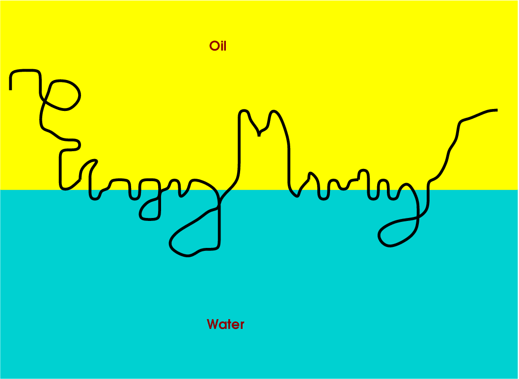
A copolymer is a polymer consisting of different types of monomers. The order of the monomers is determined by the polymerization process through which the copolymer is grown. This section looks at a $(1+1)$ -dimensional directed copolymer, consisting of a random concatenation of hydrophobic and hydrophilic monomers, near a linear interface separating two immiscible solvents, oil and water, as depicted in Fig. 31.

The copolymer has a tendency to stay close to the oil-water interface, in order to be able to place as many of its monomers in their preferred fluid. In doing so it lowers energy but loses entropy. A phase transition may be expected between a localized phase, where the copolymer stays close to the interface, and a delocalized phase, where it wanders away. Which of the two phases actually occurs depends on the strengths of the chemical affinities.

Copolymers near liquid-liquid interfaces are of interest due to their extensive application as surfactants, emulsifiers, and foaming or antifoaming agents. Many fats contain stretches of hydrophobic and hydrophilic monomers, arranged in some sort of erratic manner, and therefore are examples of random copolymers. (For the description of such systems, the undirected version of the model depicted in Fig. 32 is of course more appropriate, but we restrict ourselves to the directed version because this is mathematically much more tractable.) The transition between a localized and a delocalized phase has been observed experimentally, e.g. in neutron reflection studies of copolymers consisting of blocks of ethylene oxide and propylene oxide near a hexane-water interface. Here, a thin layer of hexane, approximately $10^{-5}\,\mbox{m}$ thick, is spread on water. In the localized phase, the copolymer is found to stretch itself along the interface in a band of width approximately $20\,\mbox{\AA}$ .

In Sections 5.1–5.4 we define and study the copolymer model. In Section 5.5 we look at a version of the copolymer model where the linear interface is replaced by a random interface, modelling a micro-emulsion. Section 5.6 lists some open problems.

5.1. Model

Let

{\mathcal{W}}_{n}=\big\{w=(i,w_{i})_{i=0}^{n}\colon\,w_{0}=0,\,w_{i+1}-w_{i}=\pm 1\,\,\forall\,0\leq i<n\big\}

denote the set of all $n$ -step directed paths that start from the origin and at each step move either north-east or south-east. Let

\omega=(\omega_{i})_{i\in{\mathbb{N}}}\mbox{ be i.i.d.\ with }{\mathbb{P}}(\omega_{1}=+1)={\mathbb{P}}(\omega_{1}=-1)=\tfrac{1}{2}

label the order of the monomers along the copolymer. Write ${\mathbb{P}}$ to denote the law of $\omega$ . The Hamiltonian, for fixed $\omega$ , is

H_{n}^{\beta,h,\omega}(w)=-\beta\sum_{i=1}^{n}(\omega_{i}+h)\,{\rm sign}(w_{i-1},w_{i}),\qquad w\in{\mathcal{W}}_{n},

with $\beta,h\in[0,\infty)$ the disorder strength, respectively, the disorder bias (the meaning of ${\rm sign}(w_{i-1},w_{i})$ is explained below). The path measure, for fixed $\omega$ , is

P_{n}^{\beta,h,\omega}(w)=\frac{1}{Z_{n}^{\beta,h,\omega}}\,{\mathrm{e}}^{-H_{n}^{\beta,h,\omega}(w)}\,P_{n}(w),\qquad w\in{\mathcal{W}}_{n},

where $P_{n}$ is the law of the $n$ -step directed random walk, which is the uniform distribution on ${\mathcal{W}}_{n}$ . Note that $P_{n}$ is the projection on ${\mathcal{W}}_{n}$ of the law $P$ of the infinite directed walk whose vertical steps are ${\rm SRW}$ .

The interpretation of the above definitions is as follows: $\omega_{i}=+1$ or $-1$ stands for monomer $i$ being hydrophobic or hydrophilic; ${\rm sign}(w_{i-1},w_{i})=+1$ or $-1$ stands for monomer $i$ lying in oil or water; $-\beta(\omega_{i}+h){\rm sign}(w_{i-1},w_{i})$ is the energy of monomer $i$ . For $h=0$ both monomer types interact equally strongly, while for $h=1$ the hydrophilic monomers do not interact at all. Thus, only the regime $h\in[0,1]$ is relevant, and for $h>0$ the copolymer prefers the oil over the water.

Note that the energy of a path is a sum of contributions coming from its successive excursions away from the interface (this viewpoint was already exploited in Section 4 for the random pinning model). All that is relevant for the energy of the excursions is what stretch of $\omega$ they sample, and whether they are above or below the interface. The copolymer model is harder than the random pinning model, because the energy of an excursion depends on the sum of the values of $\omega$ in the stretch that is sampled, not just on the first value. We expect the localized phase to occur for large $\beta$ and/or small $h$ and the delocalized phase for small $\beta$ and/or large $h$ . Our goal is to identify the critical curve separating the two phases.

5.2. Free energies

The quenched free energy is defined as

f^{\mathrm{que}}(\beta,h)=\lim_{n\to\infty}\frac{1}{n}\log Z_{n}^{\beta,h,\omega}\qquad\omega{\rm-a.s.}

Subadditivity arguments show that $\omega$ -a.s. the limit exists and is non-random for all $\beta,h\in[0,\infty)$ (see Tutorial 1 in Appendix A). The following lower bound holds:

f^{\mathrm{que}}(\beta,h)\geq\beta h\qquad\forall\,\beta,h\in[0,\infty).

Proof.

Abbreviate

\Delta_{i}={\rm sign}(S_{i-1},S_{i})

and write

	$\displaystyle Z_{n}^{\beta,h,\omega}$	$\displaystyle=E\left(\exp\left[\beta\sum_{i=1}^{n}(\omega_{i}+h)\Delta_{i}\right]\right)$
		$\displaystyle\geq E\left(\exp\left[\beta\sum_{i=1}^{n}(\omega_{i}+h)\Delta_{i}\right]\,1_{\{\Delta_{i}=+1\,\,\forall\,1\leq i\leq n\}}\right)$
		$\displaystyle=\exp\left[\beta\sum_{i=1}^{n}(\omega_{i}+h)\right]\,P(\Delta_{i}=+1\,\,\forall\,1\leq i\leq n)$
		$\displaystyle=\exp[\beta hn+o(n)+O(\log n)]\qquad\omega{\rm-a.s.},$

where the last line uses the strong law of large numbers for $\omega$ and the fact that $P(\Delta_{i}=+1\,\,\forall\,1\leq i\leq n)\geq C/n^{1/2}$ for some $C>0$ . ∎

Put

g^{\mathrm{que}}(\beta,h)=f^{\mathrm{que}}(\beta,h)-\beta h.

The above proof shows that $g^{\mathrm{que}}(\beta,h)=0$ corresponds to the strategy where the copolymer wanders away from the interface in the upward direction. This fact motivates the definition

	$\displaystyle{\mathcal{L}}$	$\displaystyle=\{(\beta,h)\colon\,g^{\mathrm{que}}(\beta,h)>0\},$
	$\displaystyle{\mathcal{D}}$	$\displaystyle=\{(\beta,h)\colon\,g^{\mathrm{que}}(\beta,h)=0\},$

referred to as the localized phase, respectively, the delocalized phase. The associated quenched critical curve is

h_{c}^{\mathrm{que}}(\beta)=\inf\{h\in[0,\infty)\colon\,g^{\mathrm{que}}(\beta,h)=0\},\quad\beta\in[0,\infty).

Convexity of $(\beta,t)\mapsto g^{\mathrm{que}}(\beta,t/\beta)$ implies that $\beta\mapsto\beta h_{c}^{\mathrm{que}}(\beta)$ is convex. It is easy to check that both are finite and therefore also continuous. Furthermore, $h_{c}^{\mathrm{que}}(0)=0$ and $h_{c}^{\mathrm{que}}(\beta)>0$ for $\beta>0$ (see below). For fixed $h$ , $\beta\mapsto g^{\mathrm{que}}(\beta,h)$ is convex and non-negative, with $g^{\mathrm{que}}(0,h)=0$ , and hence is non-decreasing. Therefore $\beta\mapsto h_{c}^{\mathrm{que}}(\beta)$ is non-decreasing as well. With the help of the convexity of $\beta\mapsto\beta h_{c}^{\mathrm{que}}(\beta)$ , it is easy to show that $\beta\mapsto\beta h_{c}^{\mathrm{que}}(\beta)$ is strictly increasing (see Giacomin [55], Theorem 6.1). Moreover, $\lim_{\beta\to\infty}h_{c}^{\mathrm{que}}(\beta)=1$ (see below). A plot is given in Fig. 33.

Figure 33. Qualitative picture of

\beta\mapsto h_{c}^{\mathrm{que}}(\beta)

. The details of the curve are known only partially (see below).

The following upper bound on the critical curve comes from an annealed estimate.

Theorem 5.1.

[Bolthausen and den Hollander [21]] $h_{c}^{\mathrm{que}}(\beta)\leq\frac{1}{2\beta}\,\log\cosh(2\beta)$ for all $\beta\in(0,\infty)$ .

Proof.

Estimate

	$\displaystyle g^{\mathrm{que}}(\beta,h)$	$\displaystyle=\lim_{n\to\infty}\frac{1}{n}\,{\mathbb{E}}\left(\log\left[{\mathrm{e}}^{-\beta hn}Z_{n}^{\beta,h,\omega}\right]\right)$
		$\displaystyle=\lim_{n\to\infty}\frac{1}{n}\,{\mathbb{E}}\left(\log E\left(\exp\left[\beta\sum_{i=1}^{n}(\omega_{i}+h)(\Delta_{i}-1)\right]\right)\right)$
		$\displaystyle\leq\lim_{n\to\infty}\frac{1}{n}\log E\left({\mathbb{E}}\left(\exp\left[\beta\sum_{i=1}^{n}(\omega_{i}+h)(\Delta_{i}-1)\right]\right)\right)$
		$\displaystyle=\lim_{n\to\infty}\frac{1}{n}\log E\left(\prod_{i=1}^{n}\left[\tfrac{1}{2}e^{-2\beta(1+h)}+\tfrac{1}{2}e^{-2\beta(-1+h)}\right]^{1_{\{\Delta_{i}=-1\}}}\right).$

The right-hand side is $\leq 0$ as soon as the term between square brackets is $\leq 1$ . Consequently,

(2\beta)^{-1}\log\cosh(2\beta)<h\quad\longrightarrow\quad g^{\mathrm{que}}(\beta,h)=0.

∎

The following lower bound comes from strategies where the copolymer dips below the interface during rare long stretches in $\omega$ where the empirical mean is sufficiently biased downwards.

Theorem 5.2.

[Bodineau and Giacomin[17]] $h_{c}^{\mathrm{que}}(\beta)\geq(\frac{4}{3}\beta)^{-1}\log\cosh(\frac{4}{3}\beta)$ for all $\beta\in(0,\infty)$ .

Proof.

See Tutorial 5 in Appendix E. ∎

Theorems 5.1–5.2 are summarized in Fig. 34.

Figure 34. Upper and lower bounds on

\beta\mapsto h_{c}^{\mathrm{que}}(\beta)

Toninelli [101], Toninelli [102], Bodineau, Giacomin, Lacoin and Toninelli [18] show that the upper and lower bounds on $h_{c}^{\mathrm{que}}(\beta)$ are strict. In fact, the strict inequalities can be extended to the setting considered in Section 4: arbitrary disorder with a finite moment-generating function and excursion length distributions that are regularly varying at infinity). Bolthausen, den Hollander and Opoku [22] derive a variational expression for $h_{c}^{\mathrm{que}}(\beta)$ , similar in spirit to what was done in Section 4.4, and extend the strict inequalities to excursion length distributions that are logarithmically equivalent to a power law.

5.3. Weak interaction limit

Theorem 5.3.

[Boltausen and den Hollander [21]] There exists a $K_{c}\in(0,\infty)$ such that

\lim_{\beta\downarrow 0}\frac{1}{\beta}\,h_{c}^{\mathrm{que}}(\beta)=K_{c}.

The idea behind this result is that, as $\beta,h\downarrow 0$ , the excursions away from the interface become longer and longer (entropy gradually takes over from energy). As a result, both $w$ and $\omega$ can be approximated by Brownian motions. In essence, the weak interaction result follows from the scaling property

\lim_{\epsilon\downarrow 0}\epsilon^{-2}\,f^{\mathrm{que}}(\epsilon\beta,\epsilon h)=\widetilde{f}^{\mathrm{que}}(\beta,h),\qquad\beta,h\geq 0,

where $\widetilde{f}^{\mathrm{que}}(\beta,h)$ is the quenched free energy of a space-time continuous version of the copolymer model, with Hamiltonian

H_{t}^{\beta,h,b}(B)=-\beta\int_{0}^{t}({\mathrm{d}}b_{s}+h\,{\mathrm{d}}s)\,\,{\rm sign}(B_{s})

and with path measure given by

\frac{{\mathrm{d}}P_{t}^{\beta,h,b}}{{\mathrm{d}}P}(B)=\frac{1}{Z_{t}^{\beta,h,b}}\,{\mathrm{e}}^{-H_{t}^{\beta,h,b}(B)},

where $B=(B_{s})_{s\geq 0}$ is the polymer path, $P$ is the Wiener measure, and $b=(b_{s})_{s\geq 0}$ is a Brownian motion that plays the role of the quenched disorder. The proof is based on a coarse-graining argument. Due to the presence of exponential weight factors, the above scaling property is much more delicate than the standard invariance principle relating ${\rm SRW}$ and Brownian motion.

For the continuum model, a standard scaling argument shows that the quenched critical curve is linear. Its slope $K_{c}$ is not known and has been the subject of heated debate. The bounds in Theorems 5.1–5.2 imply that $K_{c}\in[\frac{2}{3},1]$ . Toninelli [102] proved that $K_{c}<1$ . Caravenna, Giacomin and Gubinelli [28] did simulations and found that $K_{c}\in[0.82,0.84]$ . Moreover, Caravenna, Giacomin and Gubinelli [28] and Sohier (private communication) found that

h_{c}^{\mathrm{que}}(\beta)\approx\frac{1}{2K_{c}\beta}\,\log\cosh(2K_{c}\beta)

is a good approximation for small and moderate values of $\beta$ .

The Brownian model describes a continuum copolymer where each infinitesimal element has a random degree of “hydrophobicity” or “hydrophilicity”. It turns out that the continuum model is the scaling limit of a whole class of discrete models (see Caravenna and Giacomin [27], Caravenna, Giacomin and Toninelli [29]), i.e., there is universality. This property actually holds for a one-parameter family of continuum models indexed by a tail exponent $a\in(0,1)$ , of which the Brownian copolymer is the special case corresponding to $a=\tfrac{1}{2}$ . It is known that the above approximation of the critical curve is not an equality in general. Bolthausen, den Hollander and Opoku [22] obtain sharp upper and lower bounds on $K_{c}$ .

A related coarse-graining result is proved in Pétrélis [91] for a copolymer model with additional random pinning in a finite layer around the interface (of the type considered in Section 4). It is shown that the effect of the disorder in the layer vanishes in the weak interaction limit, i.e., only the disorder along the copolymer is felt in the weak interaction limit.

5.4. Qualitative properties of the phases

We proceed by stating a few path properties in the two phases.

Theorem 5.4.

[Biskup and den Hollander [16], Giacomin and Toninelli [58, 61]] (a) If $(\beta,h)\in{\mathcal{L}}$ , then the path intersects the interface with a strictly positive density, while the length and the height of the largest excursion away from the interface up to time $n$ is order $\log n$ .
(b) If $(\beta,h)\in{\rm int}({\mathcal{D}})$ , then the path intersects the interface with zero density. The number of intersections is $O(\log n)$ .

For $(\beta,h)\in{\rm int}({\mathcal{D}})$ , the number of intersections is expected to be $O(1)$ under the average quenched path measure (see Part III of Section 1.5). So far this has only been proved for $(\beta,h)$ above the annealed upper bound.

Theorem 5.5.

[Giacomin and Toninelli [59, 60]] For every $\beta\in(0,\infty)$ ,

0\leq g^{\mathrm{que}}(\beta,h)=O\left([h_{c}^{\mathrm{que}}(\beta)-h]^{2}\right)\qquad\mbox{ as }h\uparrow h_{c}^{\mathrm{que}}(\beta).

Theorem 5.6.

[Giacomin and Toninelli [61]] $(\beta,h)\mapsto f^{\mathrm{que}}(\beta,h)$ is infinitely differentiable on ${\mathcal{L}}$ .

Theorem 5.5 says that the phase transition is at least second order, while Theorem 5.6 says that the critical curve is the only location where a phase transition of finite order occurs. Theorem 5.5 is proved in Tutorial 5 in Appendix E.

All of the results in Sections 5.2–5.4 extend to $\omega_{i}\in{\mathbb{R}}$ rather than $\omega_{i}\in\{-1,+1\}$ , provided the law of $\omega_{i}$ has a finite moment-generating function, and to more general excursion length distributions, of the type considered in Section 4.1. For an overview, see Caravenna, Giacomin and Toninelli [29].

5.5. A copolymer in a micro-emulsion

What happens when the linear interface is replaced by a random interface? In particular, what happens when the oil forms droplets that float around in the water, as in Fig. 35? An example is milk, which is a micro-emulsion consisting (among others) of water and tiny fat-droplets. Milk is stabilized by a protein called casein, a copolymer that wraps itself around the droplets and prevents them to coagulate.

A phase transition may be expected between a localized phase, where the copolymer spends most of its time near the boundary of the droplets and makes rapid hops from one droplet to the other, and a delocalized phase, where it spends most of its time inside and outside of droplets. We will see that the actual behavior is rather more complicated. This is due to the fact that there are three (!) types of randomness in the model: a random polymer path, a random ordering of monomer types, and a random arrangement of droplets in the emulsion.

Here is a quick definition of a model. Split ${\mathbb{Z}}^{2}$ into square blocks of size $L_{n}$ . The copolymer follows a directed self-avoiding path that is allowed to make steps $\uparrow,\downarrow,\rightarrow$ and to enter and exit blocks at diagonally opposite corners (see Fig. 36). Each monomer has probability $\frac{1}{2}$ to be hydrophobic and probability $\tfrac{1}{2}$ to be hydrophilic, labeled by $\omega$ . Each block has probability $p$ to be filled with oil and probability $1-p$ to be filled with water, labeled by $\Omega$ . Assign energies $-\alpha$ and $-\beta$ to the matches hydrophobic/oil, respectively, hydrophilic/water and energy $0$ to the mismatches.

The above model was studied in den Hollander and Whittington [75], den Hollander and Pétrélis [71, 72, 73]. The key parameter ranges are $p\in(0,1)$ , $\alpha,\beta\in(0,\infty)$ , $|\beta|\leq\alpha$ . The model is studied in the limit

\lim_{n\to\infty}L_{n}=\infty,\qquad\lim_{n\to\infty}\tfrac{1}{n}L_{n}=0.

This is a coarse-graining limit in which the polymer scale and the emulsion scale separate. In this limit both scales exhibit self-averaging.

Theorems 5.7–5.8 below summarize the main results (in qualitative language), and are illustrated by Figs. 37–40.

Figure 37. Phase diagram in the supercritical regime.

Figure 39. Phase diagram in the subcritical regime.

Theorem 5.7.

[den Hollander and Whittington [75]] The free energy exists and is non-random $\omega,\Omega$ -a.s., and is given by a variational formula involving the free energies of the copolymer in each of the four possible pairs of adjacent blocks, the frequencies at which the copolymer visits these pairs on the emulsion scale, and the fractions of time the copolymer spends in these pairs on the polymer scale.

Theorem 5.8.

[den Hollander and Whittington [75], den Hollander and Pétrélis [71, 72, 73]] The analysis of the variational formula reveals that there are two regimes:
(I) Supercritical: the oil blocks percolate. There are two phases separated by one critical curve.
(II) Subcritical: the oil blocks do not percolate. There are four phases separated by three critical curves meeting in two tricritical points.

As shown in Figs. 37–40, the copolymer-emulsion model shows a remarkably rich phase behavior and associated path behavior. In the supercritical regime the phase diagram shows one critical curve separating two phases. There is a delocalized phase ${\mathcal{D}}$ where the copolymer lies entirely inside the infinite oil cluster, and a localized phase ${\mathcal{L}}$ where part of the copolymer lies near the boundary of the infinite oil cluster. In the subcritical regime the phase diagram shows three critical curves separating four phases meeting at two tricritical points. There are two delocalized phases ${\mathcal{D}}_{1}$ , ${\mathcal{D}}_{2}$ and two localized phases ${\mathcal{L}}_{1}$ , ${\mathcal{L}}_{2}$ . For each pair, the distinction comes from the way in which the copolymer behaves near the boundary of the finite oil clusters.

The corner restriction is unphysical, but makes the model mathematically tractable. In den Hollander and Pétrélis [74] this restriction is removed, but the resulting variational formula for the free energy is more complex. The coarse-graining limit is an important simplification: mesoscopic disorder is easier to deal with than microscopic disorder. An example of a model with microscopic disorder in space-time will be the topic of Section 6.

5.6. Open problems

Here are some challenges:

•

For the copolymer model in Sections 5.1–5.4, prove that throughout the interior of the delocalized phase the path intersects the interface only finitely often under the average quenched path measure.
•

Determine whether the phase transition is second order or higher order.
•

Compute the critical slope $K_{c}$ of the Brownian copolymer.
•

For the copolymer/emulsion model in Section 5.5, determine the fine details of the phase diagrams in Figs. 37 and 39, and of the path properties in Figs. 38 and 40.

6. A polymer in a random potential

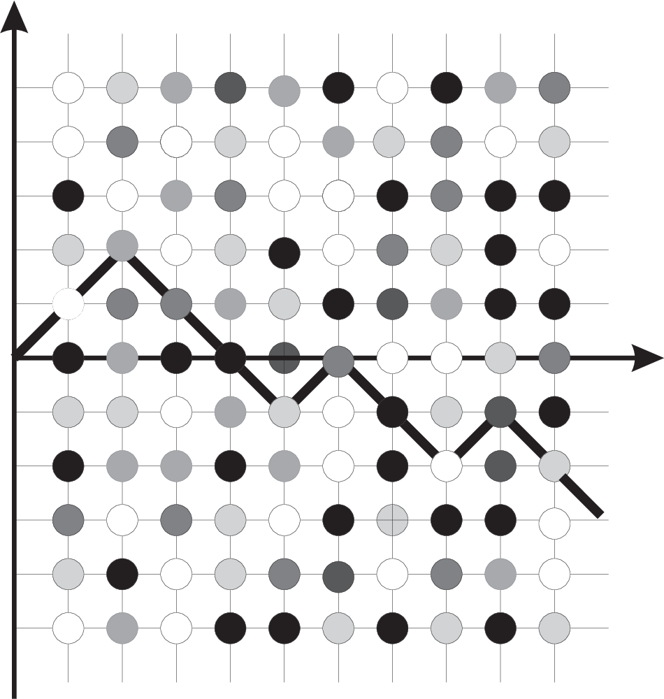
This section takes a look at a $(1+d)$ -dimensional directed polymer in a random potential: the polymer and the potential live on ${\mathbb{N}}\times{\mathbb{Z}}^{d}$ , where ${\mathbb{N}}$ is time and ${\mathbb{Z}}^{d}$ , $d\geq 1$ , is space (see Fig. 41). In Section 6.1 we define the model. In Sections 6.2–6.4 we study the two phases that occur: the weak disorder phase, in which the polymer largely ignores the disorder and behaves diffusively, and the strong disorder phase, in which the polymer hunts for favorable spots in the disorder and behaves superdiffusively. In Section 6.5 we derive bounds on the critical temperature separating the two phases. Section 6.6 lists a few open problems.

6.1. Model

The set of paths is

	$\displaystyle{\mathcal{W}}_{n}$	$\displaystyle=\big\{w=(i,w_{i})_{i=0}^{n}\colon$
		$\displaystyle w_{0}=0,\,\\|w_{i+1}-w_{i}\\|=1\,\,\forall\,0\leq i<n\big\}.$

The random environment

\omega=\{\omega(i,x)\colon\,i\in{\mathbb{N}},\,x\in{\mathbb{Z}}^{d}\}

consists of an i.i.d. field of ${\mathbb{R}}$ -valued non-degenerate random variables with moment generating function

M(\beta)={\mathbb{E}}\big({\mathrm{e}}^{\beta\omega(1,0)}\big)<\infty\qquad\forall\,\beta\in[0,\infty),

where ${\mathbb{P}}$ denotes the law of $\omega$ . The Hamiltonian is

H_{n}^{\beta,\omega}(w)=-\beta\sum_{i=1}^{n}\omega(i,w_{i}),\qquad w\in{\mathcal{W}}_{n},

where $\beta$ plays the role of the disorder strength. The associated quenched path measure is

P_{n}^{\beta,\omega}(w)=\frac{1}{Z_{n}^{\beta,\omega}}\,{\mathrm{e}}^{-H_{n}^{\beta,\omega}(w)}\,P_{n}(w),\qquad w\in{\mathcal{W}}_{n},

where $P_{n}$ is the projection onto ${\mathcal{W}}_{n}$ of the law $P$ of directed ${\rm SRW}$ on ${\mathbb{Z}}^{d}$ .

We may think of the model as a version of the “copolymer in emulsion” described in Section 5.5 where the disorder is microscopic rather than mesoscopic. There are deep relations with several other models in probability theory and statistical physics, including growth and wave-front-propagation models and first-passage percolation. Indeed, for $\beta=\infty$ the polymer follows the path along which the sum of the disorder is largest. This case corresponds to oriented first-passage percolation, of which some aspects are discussed in the lectures by Garban and Steif [54]. For $\beta<\infty$ the model is sometimes referred to as oriented first-passage percolation at positive temperature.

The key object in the analysis of the model is the following quantity:

Y_{n}^{\beta,\omega}=\frac{Z_{n}^{\beta,\omega}}{{\mathbb{E}}(Z_{n}^{\beta,\omega})},\qquad n\in{\mathbb{N}}_{0}.

This is the ratio of the quenched and the annealed partition sum. The point is that

(Y_{n}^{\beta,\omega})_{n\in{\mathbb{N}}_{0}}

is a martingale w.r.t. the natural filtration generated by $\omega$ , i.e., ${\mathcal{F}}=({\mathcal{F}}_{n})_{n\in{\mathbb{N}}_{0}}$ with ${\mathcal{F}}_{n}=\sigma(\omega(i,x)\colon\,0\leq i\leq n,\,x\in{\mathbb{Z}}^{d})$ . Indeed, this is seen by writing

Y_{n}^{\beta,\omega}=E\left(\prod_{i=1}^{n}\left[\frac{{\mathrm{e}}^{\beta\omega(i,S_{i})}}{M(\beta)}\right]\right),\qquad Y_{0}^{\beta,\omega}=1,

from which it is easily deduced that ${\mathbb{E}}(Y_{n}^{\beta,\omega}|{\mathcal{F}}_{n-1})=Y_{n-1}^{\beta,\omega}$ . Note that ${\mathbb{E}}(Y_{n}^{\beta,\omega})=1$ and $Y_{n}^{\beta,\omega}>0$ for all $n\in{\mathbb{N}}_{0}$ .

6.2. A dichotomy: weak and strong disorder

Since $Y_{n}^{\beta,\omega}\geq 0$ , it follows from the martingale convergence theorem that

Y^{\beta,\omega}=\lim_{n\to\infty}Y_{n}^{\beta,\omega}\quad\mbox{exists }\omega\text{-a.s.}

Moreover, since the event $\{\omega\colon\,Y^{\beta,\omega}>0\}$ is measurable w.r.t. the tail sigma-algebra of $\omega$ , it follows from the Kolmogorov zero-one law that the following dichotomy holds:

\begin{array}[]{lll}&\mathrm{({\rm WD})}\colon&\quad{\mathbb{P}}(Y^{\beta,\omega}>0)=1,\\ &\mathrm{({\rm SD})}\colon&\quad{\mathbb{P}}(Y^{\beta,\omega}=0)=1.\end{array}

In what follows it will turn out that $\mathrm{(WD)}$ characterizes weak disorder, for which the behavior of the polymer is diffusive in the ${\mathbb{Z}}^{d}$ -direction, while $\mathrm{(SD)}$ characterizes strong disorder, for which the behavior is (expected to be) superdiffusive (see Fig. 42). Note that the nomenclature is appropriate: in phase $\mathrm{(WD)}$ the quenched and the annealed partition sum remain comparable in the limit as $n\to\infty$ , indicating a weak role for the disorder, while in phase $\mathrm{(SD)}$ the annealed partition sum grows faster than the quenched partition sum, indicating a strong role for the disorder.

6.3. Separation of the two phases

Theorem 6.1.

[Comets and Yoshida [42]] For any choice of the disorder distribution, $\beta\mapsto{\mathbb{E}}(\sqrt{Y^{\beta,\omega}})$ is non-increasing on $[0,\infty)$ . Consequently, there exists a $\beta_{c}\in[0,\infty]$ such that (see Fig. 43)

	$\displaystyle\beta\in[0,\beta_{c})$	$\displaystyle\longrightarrow\quad\mathrm{(WD)},$
	$\displaystyle\beta\in(\beta_{c},\infty)$	$\displaystyle\longrightarrow\quad\mathrm{(SD)}.$

Figure 43. Separation of the two phases. It is not known which of the two phases includes

\beta_{c}

Since

	$\displaystyle f^{\mathrm{que}}(\beta)$	$\displaystyle=\lim_{n\to\infty}\frac{1}{n}\log Z_{n}^{\beta,\omega}\qquad\omega\text{-a.s.},$
	$\displaystyle f^{\mathrm{ann}}(\beta)$	$\displaystyle=\lim_{n\to\infty}\frac{1}{n}\log{\mathbb{E}}(Z_{n}^{\beta,\omega}),$

it follows from the above theorem that

f^{\mathrm{que}}(\beta)=f^{\mathrm{ann}}(\beta)\qquad\forall\,\beta\in[0,\beta_{c}],

where the critical value $\beta=\beta_{c}$ can be added because free energies are continuous. It is expected that (see Fig. 44)

f^{\mathrm{que}}(\beta)<f^{\mathrm{ann}}(\beta)\qquad\forall\,\beta\in(\beta_{c},\infty),

so that for $\beta\in(\beta_{c},\infty)$ the quenched and the annealed partition sum have different exponential growth rates, but this remains open. Partial results have been obtained in Comets and Vargas [39], Lacoin [83].

Figure 44. Conjectured behavior of the quenched and the annealed free energy.

6.4. Characterization of the two phases

Let

\pi_{d}=(P\otimes P^{\prime})(\exists\,n\in{\mathbb{N}}\colon\,S_{n}=S^{\prime}_{n})

denote the collision probability of two independent copies of ${\rm SRW}$ . Note that $\pi_{d}=1$ in $d=1,2$ and $\pi_{d}<1$ in $d\geq 3$ . For $\beta\in[0,\infty)$ , define

	$\displaystyle\Delta_{1}(\beta)$	$\displaystyle=\log[M(2\beta)/M(\beta)^{2}],$
	$\displaystyle\Delta_{2}(\beta)$	$\displaystyle=\beta[\log M(\beta)]^{\prime}-\log M(\beta).$

Both $\beta\mapsto\Delta_{1}(\beta)$ and $\beta\mapsto\Delta_{2}(\beta)$ are strictly increasing on $[0,\infty)$ , with $\Delta_{1}(0)=\Delta_{2}(0)=0$ and $\Delta_{1}(\beta)>\Delta_{2}(\beta)$ for $\beta\in(0,\infty)$ .

Define

\mathrm{max}_{n}^{\beta,\omega}=\max_{x\in{\mathbb{Z}}^{d}}P_{n}^{\beta,\omega}(S_{n}=x),\qquad n\in{\mathbb{N}}.

This quantity measures how localized the endpoint $S_{n}$ of the polymer is in the given potential $\omega$ : if $\lim_{n\to\infty}\mathrm{max}_{n}^{\beta,\omega}=0$ , then the path spreads out, while if $\limsup_{n\to\infty}\mathrm{max}_{n}^{\beta,\omega}>0$ , then the path localizes (at least partially).

Theorem 6.2.

[Imbrie and Spencer [76], Bolthausen [19], Sinai [95], Carmona and Hu [33], Comets, Shiga and Yoshida [37]] Suppose that

$\mathrm{(I)}$

$d\geq 3$ , $\Delta_{1}(\beta)<\log(1/\pi_{d})$ .

Then

\lim_{n\to\infty}\frac{1}{n}\,E_{n}^{\beta,\omega}(\|S_{n}\|^{2})=1\qquad\omega\text{-a.s.}

and

\lim_{n\to\infty}\,\mathrm{max}_{n}^{\beta,\omega}=0\qquad\omega\text{-a.s.}

Theorem 6.3.

[Carmona and Hu [33], Comets, Shiga and Yoshida [37]] Suppose that

$\mathrm{(II)}$

$d=1,2$ , $\beta>0$ or $d\geq 3$ , $\Delta_{2}(\beta)>\log(2d)$ .

Then there exists a $c=c(d,\beta)>0$ such that

\limsup_{n\to\infty}\,\mathrm{max}_{n}^{\beta,\omega}\geq c\qquad\omega\text{-a.s.}

Theorems 6.2–6.3 show that the polymer has qualitatively different behavior in the two regimes. In (I), the scaling is diffusive, with the diffusion constant not renormalized by the disorder. The reason why the diffusion constant is not renormalized is the directedness of the path: this causes the annealed model to be directed ${\rm SRW}$ . In (II), there is certainly no scaling to Brownian motion, due to the presence of atoms: the endpoint of the polymer concentrates around one or more most favorable sites whose locations depend on $\omega$ . These locations are expected to be at a distance much larger than $\sqrt{n}$ , i.e., the scaling is predicted to be superdiffusive. This has, however, only been proved in some special cases, in particular, for a one-dimensional model of a directed polymer in a Gaussian random environment (Petermann [88]). Further results, also for related models, have been obtained in Piza [92], Méjane [87], Carmona and Hu [34], Bezerra, Tindel and Viens [10] and Lacoin [85]. The latter reference contains a discussion of the physical conjectures and the mathematical results on this topic.

The proofs of Theorems 6.2–6.3 are based on a series of technical estimates for the martingale $(Y_{n}^{\beta,\omega})_{n\in{\mathbb{N}}_{0}}$ . These estimates also show that

\mathrm{(I)}\longrightarrow\mathrm{({\rm WD})},\qquad\mathrm{(II)}\longrightarrow\mathrm{({\rm SD})}.

It has been conjectured that, throughout phase (SD),

E_{n}^{\beta,\omega}(\|S_{n}\|^{2})\asymp n^{2\nu}\quad n\to\infty,\,\omega-a.s.

( $\asymp$ means modulo logarithmic factors), where the exponent $\nu$ is predicted not to depend on $\beta$ and to satisfy

\nu=\tfrac{2}{3}\mbox{ for }d=1,\qquad\nu\in(\tfrac{1}{2},\tfrac{2}{3})\mbox{ for }d=2,

signalling superdiffusive behavior.

6.5. Bounds on the critical temperature

Theorems 6.2–6.3 show that $\beta_{c}=0$ for $d=1,2$ and $\beta_{c}\in(0,\infty]$ for $d\geq 3$ (because $\Delta_{1}(0)=0$ and $\pi_{d}<1$ ). However, there is a gap between regimes (I) and (II) in $d\geq 3$ (because $\pi_{d}>1/2d$ and $\Delta_{1}(\beta)>\Delta_{2}(\beta)$ for all $\beta>0$ ). Thus, the results do not cover the full parameter regime. In fact, all we know is that

\beta_{c}\in[\beta_{c}^{1},\beta_{c}^{2}].

with (see Fig. 45)

	$\displaystyle\beta_{c}^{1}$	$\displaystyle=\sup\big\{\beta\in[0,\infty)\colon\,\Delta_{1}(\beta)<\log(1/\pi_{d})\big\},$
	$\displaystyle\beta_{c}^{2}$	$\displaystyle=\inf\big\{\beta\in[0,\infty)\colon\,\Delta_{2}(\beta)>\log(2d)\big\}.$

Figure 45. For

d\geq 3

three cases are possible depending on the law

{\mathbb{P}}

of the disorder: (1)

0<\beta_{c}^{1}<\beta_{c}^{2}<\infty

; (2)

0<\beta_{c}^{1}<\beta_{c}^{2}=\infty

; (3)

\beta_{c}^{1}=\beta_{c}^{2}=\infty

Various attempts have been made to sharpen the estimates on $\beta_{c}$ : fractional moment estimates on the martingale (Evans and Derrida [52], Coyle [44], Camanes and Carmona [24]); size-biasing of the martingale (Birkner [11]). We describe the latter estimate, which involves a critical threshold $z^{*}$ associated with the collision local time of two independent ${\rm SRW}$ s.

Theorem 6.4.

[Birkner [11]] Let

z^{*}=\sup\big\{z\geq 1\colon\,E\big(z^{V(S,S^{\prime})}\big)<\infty\,\,S^{\prime}-a.s.\big\},

where

V(S,S^{\prime})=\sum_{n\in{\mathbb{N}}}1_{\{S_{n}=S^{\prime}_{n}\}}

is the collision local time of two independent ${\rm SRW}$ s, and $E$ denotes expectation over $S$ . Define

\beta_{c}^{*}=\sup\big\{\beta\in[0,\infty)\colon\,M(2\beta)/M(\beta)^{2}<z^{*}\big\}.

Then

\beta<\beta_{c}^{*}\quad\longrightarrow\quad{\rm(WD)}

and, consequently, $\beta_{c}\geq\beta_{c}^{*}$ .

Proof.

Abreviate

e=\{e(i,x)\}_{i\in{\mathbb{N}},x\in{\mathbb{Z}}^{d}}

with

e(i,x)={\mathrm{e}}^{\beta\omega(i,x)}/M(\beta).

Consider a size-biased version of $e$ , written

\hat{e}=\{\hat{e}(i,x)\}_{i\in{\mathbb{N}},x\in{\mathbb{Z}}^{d}},

that is i.i.d., is independent of $e$ and has law $\hat{{\mathbb{P}}}$ given by

\hat{{\mathbb{P}}}(\hat{e}(1,0)\in\,\cdot\,)={\mathbb{E}}\big(e(1,0)\,1_{\{e(1,0)\in\,\cdot\,\}}\big).

No normalization is needed because ${\mathbb{E}}(e(1,0))=1$ .

Given $S^{\prime}$ , put

\hat{e}_{S^{\prime}}=\{\hat{e}_{S^{\prime}}(i,x)\}_{i\in{\mathbb{N}},x\in{\mathbb{Z}}^{d}},

with

\hat{e}_{S^{\prime}}(i,x)=1_{\{S^{\prime}_{i}\neq x\}}\,e(i,x)+1_{\{S^{\prime}_{i}=x\}}\,\hat{e}(i,x),

i.e., size-bias $e$ to $\hat{e}$ everywhere along $S^{\prime}$ , and define

\hat{Y}_{n}^{e,\hat{e},S^{\prime}}=E\left(\prod_{i=1}^{n}\hat{e}_{S^{\prime}}(i,S_{i})\right).

This is a size-biased version of the basic martingale, which in the present notation reads

Y_{n}^{e}=E\left(\prod_{i=1}^{n}e(i,S_{i})\right).

The point of the size-biasing carried out above is that for any bounded function $f\colon\,[0,\infty)\to{\mathbb{R}}$ ,

{\mathbb{E}}\big(Y_{n}^{e}\,f(Y_{n}^{e})\big)=({\mathbb{E}}\otimes\hat{{\mathbb{E}}}\otimes E^{\prime})\Big(f\big(\hat{Y}_{n}^{e,\hat{e},S^{\prime}}\big)\Big),

where ${\mathbb{E}},\hat{{\mathbb{E}}},E^{\prime}$ denote expectation w.r.t. $e,\hat{e},S^{\prime}$ , respectively. Indeed, the latter follows from the computation

	$\displaystyle{\mathbb{E}}\big(Y_{n}^{e}\,f(Y_{n}^{e})\big)$	$\displaystyle={\mathbb{E}}\left[E^{\prime}\left(\prod_{i=1}^{n}e(i,S^{\prime}_{i})\right)\,f\left(E\left(\prod_{i=1}^{n}e(i,S_{i})\right)\right)\right]$
		$\displaystyle=E^{\prime}\left({\mathbb{E}}\left[\left(\prod_{i=1}^{n}e(i,S^{\prime}_{i})\right)\,f\left(E\left(\prod_{i=1}^{n}e(i,S_{i})\right)\right)\right]\right)$
		$\displaystyle=^{!}E^{\prime}\left(({\mathbb{E}}\otimes\hat{{\mathbb{E}}})\left[f\left(E\left(\prod_{i=1}^{n}\hat{e}_{S^{\prime}}(i,S_{i})\right)\right)\right]\right)$
		$\displaystyle=({\mathbb{E}}\otimes\hat{{\mathbb{E}}}\otimes E^{\prime})\Big(f\big(\hat{Y}_{n}^{e,\hat{e},S^{\prime}}\big)\Big),$

where the third equality uses the definition of $\hat{e}_{S^{\prime}}$ .

The above identity relates the two martingales, and implies that

		$\displaystyle(Y_{n}^{e})_{n\in{\mathbb{N}}_{0}}\mbox{ is uniformly integrable }$
		$\displaystyle\Longleftrightarrow\quad(\hat{Y}_{n}^{e,\hat{e},S^{\prime}})_{n\in{\mathbb{N}}_{0}}\mbox{ is tight}\qquad(\ast)$

(as can be seen by picking $f$ such that $\lim_{u\to\infty}f(u)=\infty$ ). However, an easy computation gives

({\mathbb{E}}\otimes\hat{{\mathbb{E}}})\Big(\hat{Y}_{n}^{e,\hat{e},S^{\prime}}\Big)=E\left(z^{\sum_{i=1}^{n}1_{\{S_{i}=S^{\prime}_{i}\}}}\right)=E\big(z^{V(S,S^{\prime})}\big)

with $z=M(2\beta)/M(\beta)^{2}$ , where the factor $2\beta$ arises because after the size-biasing the intersection sites of $S$ and $S^{\prime}$ are visited by both paths. Hence

E(z^{V(S,S^{\prime})})<\infty\quad S^{\prime}\text{-a.s.}

is enough to ensure that the r.h.s. of $(\ast)$ holds. This completes the proof because the l.h.s. of $(\ast)$ is equivalent to (WD). Indeed, a.s. convergence plus uniform integrability imply convergence in mean, so that ${\mathbb{E}}(Y_{n}^{e})=1$ for all $n\in{\mathbb{N}}_{0}$ yields ${\mathbb{E}}(Y^{e})=1$ . ∎

In Birkner, Greven and den Hollander [13] it was proved that $z^{*}>\pi_{d}$ in $d\geq 5$ , implying that $\beta_{c}^{*}>\beta_{c}^{1}$ . It was conjectured that the same is true in $d=3,4$ . Part of this conjecture was settled in Birkner and Sun [14, 15] and Berger and Toninelli [9] (see Fig. 46).

Figure 46. Bounds on the critical temperature.

6.6. Open problems

•

Show that in phase $\mathrm{(SD)}$ the polymer is concentrated inside a most favorable corridor and identify how this corridor depends on $\omega$ .
•

Determine whether $\beta_{c}$ is part of $\mathrm{(WD)}$ or $\mathrm{(SD)}$ .
•

Derive a variational expression for $\beta_{c}$ .
•

Extend the analysis to undirected random walk. Important progress has been made in Ioffe and Velenik [77, 78, 79, 80], Zygouras [104, 105], and references cited therein. See also Section 2.7.

Appendix A Tutorial 1

In this tutorial we describe two methods that can be used to prove the existence of the quenched free energy associated with the random pinning model described in Section 4. Section A.1 recalls the model, Sections A.2–A.4 prove existence of the quenched free energy when the endpoint of the polymer is constrained to lie in the interface, while Section A.5 shows how to remove this constraint afterwards. The method of proof is widely applicable, and is not specific to the random pinning model.

A.1. Random pinning of a polymer at an interface

Configurations of the polymer. Let $n\in{\mathbb{N}}$ and consider a polymer made of $n$ monomers. The allowed configurations of this polymer are modeled by the $n$ -step trajectories of a 1-dimensional random walk $S=(S_{i})_{i\in{\mathbb{N}}_{0}}$ . We focus on the case where $S_{0}=0$ and $(S_{i}-S_{i-1})_{i\in{\mathbb{N}}}$ is an i.i.d. sequence of random variables satisfying

P(S_{1}=1)=P(S_{1}=-1)=P(S_{1}=0)=\tfrac{1}{3},

although the argument given below applies more generally. We denote by ${\mathcal{W}}_{n}$ the set of all $n$ -step trajectories of $S$ .

Disorder at interface. Let $\omega=(\omega_{i})_{i\in{\mathbb{N}}}$ be an i.i.d. sequence of ${\mathbb{R}}$ -valued random variables (which we take bounded for ease of exposition). For $i\in{\mathbb{N}}$ the interaction intensity between the $i$ -th monomer and the interface takes the value $\omega_{i}$ . Note that $\omega$ and $S$ are independent, and write ${\mathbb{P}}$ for the law of $\omega$ . Pick $M>0$ such that $|\omega_{1}|\leq M$ ${\mathbb{P}}$ -a.s.

Interaction polymer-interface. The flat interface that interacts with the polymer is located at height $0$ , so that the polymer hits this interface every time $S$ comes back to $0$ . Thus, with every $S\in{\mathcal{W}}_{n}$ we associate the energy

H_{n}^{\beta,\omega}(S)=-\beta\sum_{i=0}^{n-1}\omega_{i}\,{1}_{\{S_{i}=0\}},

where $\beta\in(0,\infty)$ stands for the inverse temperature (and for ease of exposition we take zero bias, i.e., we set $h=0$ in the Hamiltonian in Section 4.1). We think of $S$ as a random realization of the path of the polymer.

Partition function and free energy. For fixed $n$ , the quenched (= frozen disorder) partition function and free energy are defined as

Z_{n}^{\beta,\omega}=E\big({\mathrm{e}}^{-H_{N}^{\beta,\omega}(S)}\big)\quad\text{and}\quad f_{n}^{\beta,\omega}=\tfrac{1}{n}\log Z_{n}^{\omega,\beta}.

A.2. Convergence of the free energy

Our goal is to prove the following theorem.

Theorem A.1.

For every $\beta\in{\mathbb{R}}$ there exists an $f(\beta)\in[0,\beta M]$ such that

\lim_{n\to\infty}{\mathbb{E}}(f_{n}^{\beta,\omega})=f(\beta)

and

\lim_{n\to\infty}f_{n}^{\beta,\omega}=f(\beta)\quad{\mathbb{P}}-a.e.\ \omega.

As indicated above, we will prove Theorem A.1 via two different methods. In Section A.3 we will state Kingman’s Subadditive Ergodic Theorem and see how this can be applied to obtain Theorem A.1. In Section A.4 we will re-prove Theorem A.1 by using a concentration of measure argument. The latter method is more involved, but also more flexible than the former method. For technical reasons, we will first prove Theorem A.1 with the partition function restricted to those trajectories that hit the interface at their right extremity, i.e.,

Z_{n}^{*,\beta,\omega}=E\big({\mathrm{e}}^{-H_{n}^{\beta,\omega}(S)}\ {1}_{\{S_{n}=0\}}\big)\quad\text{and}\quad f_{n}^{*,\beta,\omega}=\tfrac{1}{n}\log Z_{n}^{*,\beta,\omega}.

In Section A.5 we will see that the restriction on the endpoint has no effect on the value of the limiting free energy.

A.3. Method 1: Kingman’s theorem

Theorem A.2.

[Kingman’s Subadditive Ergodic Theorem; see Steele [98]] Let $(\Omega,A,\mu)$ be a probability space, let $T$ be an ergodic measure-preserving transformation acting on $\Omega$ , and let $(g_{n})_{n\in{\mathbb{N}}}$ be a sequence of random variables in $L_{1}(\mu)$ that satisfy the subadditivity relation

g_{m+n}\geq g_{m}+g_{n}(T^{m}),\qquad m,n\in{\mathbb{N}}.

Then

\lim_{n\to\infty}\frac{g_{n}}{n}=\sup_{k\in{\mathbb{N}}}E_{\mu}\left(\frac{g_{k}}{k}\right)\qquad\mu\text{-a.s.}

(1) Let $T$ be the left-shift on ${\mathbb{R}}^{\mathbb{N}}$ . Prove that, for $m,n\in{\mathbb{N}}$ and $\omega\in{\mathbb{R}}^{\mathbb{N}}$ ,

\log Z_{m+n}^{*,\beta,\omega}\geq\log Z_{m}^{*,\beta,\omega}+\log Z_{n}^{*,\beta,T^{m}(\omega)}.

(2) Apply Theorem A.2 with $(\Omega,A,\mu)=({\mathbb{R}}^{\mathbb{N}},\text{Bor}({\mathbb{R}}^{{\mathbb{N}}}),{\mathbb{P}})$ and prove Theorem A.1 with the endpoint restriction.

A.4. Method 2: Concentration of measure

This method consists of first proving the first line in Theorem A.1, i.e., the convergence of the average quenched free energy, and then using a concentration of measure inequality to show that, with large probability, the quenched free energy is almost equal to its expectation, so that the second line in Theorem A.1 follows. See Giacomin and Toninelli [58] for fine details.

(1) Use (A.3) and prove that $({\mathbb{E}}(\log Z_{n}^{*,\beta,\omega}))_{n\in{\mathbb{N}}}$ is a superadditive sequence, i.e., for $m,n\in{\mathbb{N}}$ ,

{\mathbb{E}}(\log Z_{m+n}^{*,\beta,\omega})\geq{\mathbb{E}}(\log Z_{m}^{*,\beta,\omega})+{\mathbb{E}}(\log Z_{n}^{*,\beta,\omega}).

(2) Deduce that (see also the tutorial in Appendix A.1 of Bauerschmidt, Duminil-Copin, Goodman and Slade [7])

\lim_{n\to\infty}{\mathbb{E}}(f_{n}^{*,\beta,\omega})=\sup_{k\in{\mathbb{N}}}\,{\mathbb{E}}(f_{k}^{*,\beta,\omega})=f(\beta)\in[0,\beta M].

To proceed, we need the following inequality.

Theorem A.3.

[Concentration of measure; see Ledoux [86]] There exist $C_{1},C_{2}$ $>0$ such that for all $n\in{\mathbb{N}}$ , $K>0$ , ${\varepsilon}>0$ and $G_{n}\colon\,{\mathbb{R}}^{n}\mapsto{\mathbb{R}}$ a $K$ -Lipschitz (w.r.t. the Euclidean norm) convex function,

{\mathbb{P}}\Big(\big|G_{n}(\omega_{0},\dots,\omega_{n-1})-{\mathbb{E}}\big(G_{n}(\omega_{0},\dots,\omega_{n-1})\big)\big|>{\varepsilon}\Big)\leq C_{1}{\mathrm{e}}^{-\tfrac{C_{2}{\varepsilon}^{2}}{K^{2}}}.

(3) By Hölder’s inequality, the function $\omega\in{\mathbb{R}}^{n}\mapsto f_{n}^{*,\beta,\omega}\in{\mathbb{R}}$ is convex. To prove that it is $(\beta/\sqrt{n})$ -Lipschitz, pick $\omega,\omega^{\prime}\in{\mathbb{R}}^{n}$ and compute

	$\displaystyle\left\|\frac{\partial}{\partial t}\,f_{n}^{*,\beta,t\omega+(1-t)\omega^{\prime}}\right\|$	$\displaystyle=\frac{\beta}{n}\,\left\|\sum_{i=0}^{n-1}P_{n}^{*,\beta,\omega}(S_{i}=0)\,(\omega_{i}-\omega^{\prime}_{i})\right\|$
		$\displaystyle\leq\frac{\beta}{n}\,\sqrt{\sum_{i=0}^{n-1}\big[P_{n}^{*,\beta,\omega}(S_{i}=0)\big]^{2}}\,\sqrt{\sum_{i=0}^{n-1}(\omega_{i}-\omega^{\prime}_{i})^{2}}$
		$\displaystyle\leq\frac{\beta}{\sqrt{n}}\,\sqrt{\sum_{i=0}^{n-1}(\omega_{i}-\omega^{\prime}_{i})^{2}},$

where $P_{n}^{*,\beta,\omega}$ is the path measure with the endpoint restriction.

(4) Apply Theorem A.3 to prove that, for ${\varepsilon}>0$ ,

\sum_{n\in{\mathbb{N}}}{\mathbb{P}}\big(|f_{n}^{*,\beta,\omega}-{\mathbb{E}}(f_{n}^{*,\beta,\omega})|>{\varepsilon}\big)<\infty.

(5) Combine (2) and (4) to show that, for ${\mathbb{P}}$ -a.e. $\omega$ , $f_{n}^{*,\beta,\omega}$ tends to $f(\beta)$ as $n\to\infty$ , which proves Theorem A.1 with the endpoint restriction.

A.5. Removal of the path restriction

The proof of Theorem A.1 will be completed once we show that restricting the partition function to $\{S_{n}=0\}$ does not alter the results. To that end, we denote by $\tau$ the first time at which the random walk $S$ hits the interface.

(6) Note that there exists a $C_{3}>0$ such that (see Spitzer [97], Section 1)

P(\tau=n)=\frac{C_{3}}{n^{3/2}}\,[1+o(1)]\quad\text{and}\quad P(\tau>n)=\frac{2C_{3}}{n^{1/2}}\,[1+o(1)].

(7) Consider the last hit of the interface and show that

Z_{n}^{\beta,\omega}=\sum_{j=0}^{n}Z_{j}^{*,\beta,\omega}\,P(\tau>n-j).

(8) Prove Theorem A.1 by combining (5), (6) and (7).

Appendix B Tutorial 2

The goal of this tutorial is to provide the combinatorial computation of the free energy for the directed polymer with self-attraction described in Sections 2.4–2.5 leading to Theorem 2.3. This computation is taken from Brak, Guttmann and Whittington [23]. Section B.1 recalls the model, Section B.2 proves the existence of the free energy, while Section B.3 derives a formula for the free energy with the help of generating functions.

B.1. Model of a directed polymer in a poor solvent

We begin by recalling some of the notation used in Sections 2.4–2.5.

Configurations of the polymer. For $n\in{\mathbb{N}}$ , the configurations of the polymer are modelled by $n$ -step $(1+1)$ -dimensional directed self-avoiding paths $w=(w_{i})_{i=0}^{n}$ that are allowed to move up, down and to the right, i.e.,

	$\displaystyle{\mathcal{W}}_{n}=\{(w_{i})_{i=0}^{n}\in({\mathbb{N}}_{0}\times{\mathbb{Z}})^{n+1}\colon$	$\displaystyle w_{0}=0,w_{1}-w_{0}=\rightarrow,$
		$\displaystyle w_{i}-w_{i-1}=\{\uparrow,\downarrow,\rightarrow\}\ \forall 1\leq i\leq n,$
		$\displaystyle w_{i}\neq w_{j}\ \forall\,0\leq i<j\leq n\}.$

Self-touchings. The monomers constituting the polymer have an attractive interaction: an energetic reward is given for each self-touching, i.e., for each pair $(w_{i},w_{j})$ with $i<j-1$ and $|w_{i}-w_{j}|=1$ . Accordingly, with each $w\in{\mathcal{W}}_{n}$ we associate the number of self-touchings

J_{n}(w)=\sum_{0\leq i<j-1\leq n-1}\,{1}_{\{|w_{i}-w_{j}|=1\}},

and the energy

H_{n}^{\gamma}(w)=-\gamma J_{n}(w),

where $\gamma\in{\mathbb{R}}$ is the interaction parameter.

Partition function, free energy and generating function. For fixed $n$ , the partition function and free energy are defined as

Z_{n}^{\gamma}=\sum_{w\in{\mathcal{W}}_{n}}{\mathrm{e}}^{-H_{n}^{\gamma}(w)},\qquad f_{n}(\gamma)=\tfrac{1}{n}\log Z_{n}^{\gamma}.

For $n\in{\mathbb{N}}_{0}$ and $x\in[0,\infty)$ , let

Z_{n}(x)=\sum_{m\in{\mathbb{N}}_{0}}c_{n}(m)\,x^{m},\quad c_{n}(m)=|\{w\in{\mathcal{W}}_{n}\colon\,J_{n}(w)=m\}|.

Then $Z_{n}^{\gamma}=Z_{n}({\mathrm{e}}^{\gamma})$ , and the generating function of $Z_{n}^{\gamma}$ can be written as

\sum_{n\in{\mathbb{N}}_{0}}Z_{n}^{\gamma}y^{n}=G({\mathrm{e}}^{\gamma},y)

with

G(x,y)=\sum_{n\in{\mathbb{N}}_{0}}\sum_{m\in{\mathbb{N}}_{0}}c_{n}(m)x^{m}y^{n},\qquad x,y\in[0,\infty).

B.2. Existence of the free energy

Existence comes in three steps.

(1) Show that for $m,n\in{\mathbb{N}}_{0}$ and $x\in[0,\infty)$ ,

Z_{m+n+1}(x)\geq Z_{m}(x)\,Z_{n}(x)\quad\text{and}\quad Z_{n}(x)\leq[3(1\vee x)]^{n}.

(2) Deduce that

\lim_{n\to\infty}\frac{1}{n}\log Z_{n}(x)=\sup_{k\in{\mathbb{N}}}\,\frac{1}{k}\log Z_{k}(x)=\bar{f}(x)\in(0,\log 3+(0\vee\log x)].

Thus, $f(\gamma)=\bar{f}({\mathrm{e}}^{\gamma})$ , $\gamma\in{\mathbb{R}}$ .

(3) For $x\in[0,\infty)$ , let $y_{c}(x)$ be the radius of convergence of the generating function $G(x,y)$ . Show that

(B.1)

\bar{f}(x)=-\log y_{c}(x).

B.3. Computation of the free energy

To prove Theorem 2.3, we must compute $y_{c}(x)$ , $x\in[0,\infty)$ . In what follows we derive the formula for $G(x,y)$ given in Lemma 2.4.

(1) For $n,r,s\in{\mathbb{N}}_{0}$ , let

		$\displaystyle{\mathcal{W}}_{n,r}$
		$\displaystyle=\{w\in{\mathcal{W}}_{n}\colon\;\text{$w$ makes exactly $r$ vertical steps after the first step east}\},$
		$\displaystyle{\mathcal{W}}_{n,r,s}$
		$\displaystyle=\{w\in{\mathcal{W}}_{n,r}\colon\;\text{$w$ makes exactly $s$ vertical steps after the second step east}\},$

and note that ${\mathcal{W}}_{n,r}=\emptyset$ if $n<1+r$ and ${\mathcal{W}}_{n,r,s}=\emptyset$ if $n<2+r+s$ . Furthermore, for $r,s\in{\mathbb{N}}$ , let

		$\displaystyle{\mathcal{W}}_{n,r,s}^{\,\uparrow\downarrow}$
		$\displaystyle=\{w\in{\mathcal{W}}_{n,r,s}\colon\;\text{the $r$ and $s$ vertical steps are made in opposite directions}\},$
		$\displaystyle{\mathcal{W}}_{n,r,s}^{\,\uparrow\uparrow}$
		$\displaystyle=\{w\in{\mathcal{W}}_{n,r,s}\colon\;\text{the $r$ and $s$ vertical steps are made in the same direction}\},$

so that, for $r\in{\mathbb{N}}$ , ${\mathcal{W}}_{n,r}$ can be partitioned as

{\mathcal{W}}_{n,r}=\bigcup_{s=0}^{n-r-2}{\mathcal{W}}_{n,r,s}={\mathcal{W}}_{n,r,0}\cup\left[\bigcup_{s=1}^{n-r-2}\big[{\mathcal{W}}_{n,r,s}^{\,\uparrow\downarrow}\cup{\mathcal{W}}_{n,r,s}^{\,\uparrow\uparrow}\big]\right].

For $n,r,m\in{\mathbb{N}}_{0}$ , let $c_{n,r}(m)$ be the number of $n$ -step paths with $m$ self-touchings making exactly $r$ steps north or south immediately after the first step east, and put

g_{r}(x,y)=\sum_{n\in{\mathbb{N}}_{0}}\sum_{m\in{\mathbb{N}}_{0}}c_{n,r}(m)\,x^{m}\,y^{n}.

Clearly, $G(x,y)=\sum_{r\in{\mathbb{N}}_{0}}g_{r}(x,y)$ .

(2) Pick $r\in{\mathbb{N}}$ and use the first equality in the partitioning of ${\mathcal{W}}_{n,r}$ , together with the fact that $c_{n,r}(m)=0$ when $n<r+1$ , to prove that

g_{r}(x,y)=2y^{r+1}+\sum_{s\in{\mathbb{N}}_{0}}\sum_{n=r+2+s}^{\infty}\ \sum_{w\in{\mathcal{W}}_{n,r,s}}x^{J_{n}(w)}\,y^{n}.

For $w\in{\mathcal{W}}_{n}$ and $0\leq l<s\leq n$ , let

J_{l,s}(w)=\sum_{l\leq i<j-1\leq s-1}\,{1}_{\{|w_{i}-w_{j}|=1\}},

which stands for the number of self-touchings made by $w$ between its $l$ -th and $s$ -th step. Clearly, $J_{n}(w)=J_{0,n}(w)$ .

(3) Pick $r,s\in{\mathbb{N}}$ and $n\geq r+s+2$ . Prove that

		$\displaystyle w\in{\mathcal{W}}_{n,r,s}^{\,\uparrow\uparrow}\quad\longrightarrow\quad J_{n}(w)=J_{r+1,n}(w),$
		$\displaystyle w\in{\mathcal{W}}_{n,r,s}^{\,\uparrow\downarrow}\quad\longrightarrow\quad J_{n}(w)=J_{r+1,n}(w)+\min\{r,s\}.$

(4) Use (2) and (3) to show that

(B.2)

\displaystyle g_{r}(x,y)

\displaystyle=y^{r+1}\left[2+\sum_{s=0}^{r}(1+x^{s})\,g_{s}(x,y)+\sum_{s=r+1}^{\infty}(1+x^{r})\,g_{s}(x,y)\right],\qquad r\in{\mathbb{N}}.

In the same spirit show that

(B.3)

g_{0}(x,y)=y+y\,G(x,y).

(5) Abbreviate $g_{r}=g_{r}(x,y)$ . Prove that

(B.4)

g_{r+1}-(1+x)yg_{r}-(1-x)x^{r}y^{r+2}g_{r}+xy^{2}g_{r-1}=0\qquad r\in{\mathbb{N}}.

To do so, substitute the expressions obtained for $g_{r-1}$ , $g_{r}$ and $g_{r+1}$ from (B.2) into (B.4), and isolate the terms containing $y^{2r+3}$ . The latter leads to a rewrite of the left-hand side of (B.4) as

(B.5)

x^{r}y^{2r+3}(x-1)\left[2+\sum_{s=0}^{r}(1+x^{s})g_{s}+\sum_{s=r+1}^{\infty}(1+x^{r})g_{s}\right]+x^{r}y^{r+2}(1-x)g_{r}.

Use (B.2) once more to conclude that (B.5) equals zero.

(6) From (B.4) we see that $(g_{r})_{r\in{\mathbb{N}}_{0}}$ is determined by $g_{0}$ and $g_{1}$ , while (B.3) constitutes a consistency relation that must be met by the solution of (B.4). Thus, $(g_{r})_{r\in{\mathbb{N}}_{0}}$ belongs to a two-dimensional vector space generated by any two linearly independent solutions. For this reason, we look for two particular solutions of (B.4) by making an Ansatz. Set $q=xy$ , and write $g_{r}$ in the form

(B.6)

g_{r}=\lambda^{r}\sum_{l\in{\mathbb{N}}_{0}}p_{l}\,q^{lr},\qquad r\in{\mathbb{N}},\,p_{0}=1,

where $\lambda=\lambda(y,q)$ and $p_{l}=p_{l}(\lambda,y,q)$ , $l\in{\mathbb{N}}$ , are to be determined. Substitute (B.6) into (B.4) to obtain

(B.7)			$\displaystyle\lambda^{2}-\lambda(y+q)+yq$
(B.7)			$\displaystyle+\sum_{l\in{\mathbb{N}}}q^{l(r-1)}\Big[\big(\lambda^{2}q^{2l}-\lambda(y+q)q^{l}+yq\big)p_{l}+\big(\lambda(q-y)yq^{l}\big)\,p_{l-1}\Big]=0.$

Conclude that (B.7) is satisfied when

(B.8)

p_{l}=\frac{\lambda(y-q)yq^{l}}{(\lambda q^{l}-y)(\lambda q^{l}-q)}\,p_{l-1},\qquad l\in{\mathbb{N}},

provided $\lambda$ solves the equation $\lambda^{2}-\lambda(y+q)+yq=0$ , i.e., $\lambda\in\{\lambda_{1},\lambda_{2}\}=\{y,q\}$ .

(7) Use (6) to show that $g_{r}=C_{1}g_{r,1}+C_{2}g_{r,2}$ , $r\in{\mathbb{N}}$ , where $C_{1}$ and $C_{2}$ are functions of $y,q$ and

(B.9)

g_{r,i}=g_{r,i}(x,y)=(\lambda_{i})^{r}\bigg(1+\sum_{k\in{\mathbb{N}}}\frac{(\lambda_{i})^{k}(y-q)^{k}y^{k}q^{\tfrac{1}{2}k(k+1)}}{\prod_{l=1}^{k}(\lambda_{i}q^{l}-y)(\lambda_{i}q^{l}-q)}\ q^{kr}\bigg)\qquad i=1,2,\,r\in{\mathbb{N}}_{0}.

Pick $x>1$ and $0<y<1$ such that $q=xy<1$ , and let $r\to\infty$ in (B.9). This gives

\lim_{r\to\infty}q^{-r}g_{r,1}(x,y)=0\quad\text{and}\quad\lim_{r\to\infty}q^{-r}g_{r,2}(x,y)=1.

Next, an easy computation shows that $\lim_{r\to\infty}\frac{1}{r}\log|{\mathcal{W}}_{r}|=1+\sqrt{2}$ , with $|{\mathcal{W}}_{r}|=g_{r}(1,1)$ . Pick $x>1$ and $0<y<1$ such that $q=xy<1/(1+\sqrt{2})$ , and let $r\to\infty$ in (B.2). This gives

\lim_{r\to\infty}q^{-r}g_{r}(x,y)=0,

from which it follows that $C_{2}=0$ .

(8) It remains to determine $C_{1}$ . To that end, note that, by construction, $(g_{r,1})_{r\in{\mathbb{N}}_{0}}$ satisfies (B.4) for $r=0$ as well. Use (B.3) and (B.4) to show that

(B.10)		$\displaystyle$	$\displaystyle\tfrac{1}{2}C_{1}g_{0,1}=g_{0}=y+yG,$
(B.10)			$\displaystyle C_{1}g_{1,1}=g_{1}=a+bG,$

with

a=y^{2}(2+y-xy),\quad b=y^{2}(1+x+y-xy).

Eliminate $C_{1}$ and express $G$ in terms of $g_{0,1}$ and $g_{1,1}$ , to obtain

G(x,y)=\frac{aH(x,y)-y^{2}}{bH(x,y)-y^{2}},

where

H(x,y)=y\,\frac{g_{0,1}(x,y)}{g_{1,1}(x,y)}.

This completes the proof of Lemma 2.4 with $\bar{g}_{0}=g_{0,1}$ and $\bar{g}_{1}=g_{1,1}$ .

(9) Brak, Guttmann and Whittington [23] show that the function $H(x,y)$ can be represented as a continued fraction. This representation allows for an analysis of the singularity structure of $G(x,y)$ , in particular, for a computation of $y_{c}(x)$ (the radius of convergence of the power series $y\mapsto G(x,y)$ ) for fixed $x$ . For instance, from (B.4) it is easily deduced that

G(1/y,y)=\sum_{r\in{\mathbb{N}}_{0}}g_{r}(1/y,y)=-1+\sqrt{\frac{1-y}{1-3y-y^{2}-y^{3}}}\qquad(q=1)

and this has a singularity at $y_{c}$ solving the cubic equation $1-3y-y^{2}-y^{3}=0$ . Fig. 16 gives the plot of $x\mapsto y_{c}(x)$ that comes out of the singularity analysis. As explained in Section B.3, the free energy is $f(\gamma)=-\log y_{c}({\mathrm{e}}^{\gamma})$ .

Appendix C Tutorial 3

The purpose of this tutorial is to take a closer look at the free energy of the homogeneous pinning model described in Section 3. Section C.1 recalls the model, Section C.2 computes the free energy, while Section C.3 identifies the order of the phase transition.

C.1. The model

Let $(S_{n})_{n\in{\mathbb{N}}_{0}}$ be a random walk on ${\mathbb{Z}}$ , i.e., $S_{0}=0$ and $S_{i}-S_{i-1}$ , $i\in{\mathbb{N}}$ , are i.i.d. Let $P$ denote the law of $S$ . Introducing the first return time to zero $\tau=\inf\{n\in{\mathbb{N}}\colon\,S_{n}=0\}$ , we denote by $R(\cdot)$ its distribution:

R(n)=P(\tau=n)=P\big(S_{i}\neq 0\,\,\forall\,1\leq i\leq n-1,\,S_{n}=0\big),\qquad n\in{\mathbb{N}}.

We require that $\sum_{n\in{\mathbb{N}}}R(n)=1$ , i.e., the random walk is recurrent, and we assume the following tail asymptotics for $R(\cdot)$ as $n\to\infty$ :

R(n)=\frac{c}{n^{1+a}}\,[1+o(1)],\qquad c>0,\,a\in(0,1)\cup(1,\infty).

The exclusion of $a=1$ is for simplicity (to avoid logarithmic corrections in later statements). The constant $c$ could be replaced by a slowly varying function at the expense of more technicalities, which however we avoid. We recall that, for a nearest-neighbor symmetric random walk, i.e., when $P(S_{1}=1)=P(S_{1}=-1)=p$ and $P(S_{1}=0)=1-2p$ with $p\in(0,\frac{1}{2})$ , the above tail asymptotics holds with $\alpha=\frac{1}{2}$ .

The set of allowed polymer configurations is $\mathcal{W}_{n}=\{w=(i,w_{i})_{i=0}^{n}\colon\,w_{0}=0,\,w_{i}\in{\mathbb{Z}}\,\,\forall\,0\leq i\leq n\}$ , on which we define the Hamiltonian $H_{n}^{\zeta}(w)=-\zeta L_{n}(w)$ , where $\zeta\in{\mathbb{R}}$ and

L_{n}(w)=\sum_{i=1}^{n}{1}_{\{w_{i}=0\}},\qquad w\in{\mathcal{W}}_{n},

is the so-called local time of the polymer at the interface (which has height zero). We denote by $P_{n}$ the projection of $P$ onto $\mathcal{W}_{n}$ , i.e., $P_{n}(w)=P(S_{i}=w_{i}\,\,\forall\,1\leq i\leq n)$ for $w\in\mathcal{W}_{n}$ . This is the a priori law for the non-interacting polymer. We define our polymer model as the law $P_{n}^{\zeta}$ on $\mathcal{W}_{n}$ given by

P_{n}^{\zeta}(w)=\frac{1}{Z_{n}^{\zeta}}\,{\mathrm{e}}^{-H_{n}^{\zeta}(w)}\,P_{n}(w),\qquad w\in{\mathcal{W}}_{n}.

The normalizing constant $Z_{n}^{\zeta}$ , called the partition function, is given by

Z_{n}^{\zeta}=\sum_{w\in\mathcal{W}_{n}}{\mathrm{e}}^{-H_{n}^{\zeta}(w)}\,P_{n}(w)=E_{n}\left({\mathrm{e}}^{-H_{n}^{\zeta}(w)}\right)=E\left({\mathrm{e}}^{\zeta\sum_{i=1}^{n}{1}_{\{S_{i}=0\}}}\right).

The free energy $f(\zeta)$ is defined as the limit

f(\zeta)=\lim_{n\to\infty}\frac{1}{n}\,\log Z_{n}^{\zeta},

which has been shown to exist in Tutorial 1. From a technical viewpoint it is more convenient to consider the constrained partition sum $Z_{n}^{*,\zeta}$ defined by

Z_{n}^{*,\zeta}=\sum_{{w\in\mathcal{W}_{n}}\atop{w_{n}=0}}{\mathrm{e}}^{-H_{n}^{\zeta}(w)}\,P_{n}(w)=E\left({\mathrm{e}}^{\zeta\sum_{i=1}^{n}{1}_{\{S_{i}=0\}}}\,{1}_{\{S_{n}=0\}}\right).

As shown in Tutorial 1, if we replace $Z_{n}^{\zeta}$ by $Z_{n}^{*,\zeta}$ in the definition of $f(\zeta)$ , then this does not change the value of the limit. Therefore we may focus on $Z_{n}^{*,\zeta}$ .

C.2. Computation of the free energy

We repeat in more detail the derivation of the formula for the free energy $f(\zeta)$ given in Section 3.

(1)

Prove that $Z_{n}^{*,\zeta}\geq{\mathrm{e}}^{\zeta}\,P(\tau=n)={\mathrm{e}}^{\zeta}\,R(n)$ . Deduce that $f(\zeta)\geq 0$ for every $\zeta\in{\mathbb{R}}$ .
(2)

Show that $Z_{n}^{*,\zeta}\leq 1$ for $\zeta\in(-\infty,0]$ . Deduce that $f(\zeta)=0$ for every $\zeta\in(-\infty,0]$ .
(3)

Henceforth we focus on $\zeta\in[0,\infty)$ . Define for $x\in[0,1]$ the generating function $\phi(x)=\sum_{n\in{\mathbb{N}}}R(n)\,x^{n}$ . Observe that $x\mapsto\phi(x)$ is strictly increasing with $\phi(0)=0$ and $\phi(1)=1$ . Deduce that for every $\zeta\in[0,\infty)$ there is exactly one value $r=r(\zeta)$ that solves the equation $\phi({\mathrm{e}}^{-r})={\mathrm{e}}^{-\zeta}$ . Observe that $\tilde{R}_{\zeta}(n)={\mathrm{e}}^{\zeta}\,R(n)\,{\mathrm{e}}^{-r(\zeta)n}$ defines a probability distribution on ${\mathbb{N}}$ .

(4)

For $n\in{\mathbb{N}}$ and $1\leq k\leq n$ , denote by $\Theta_{n,k}$ the set consisting of $k+1$ points drawn from the interval $\{0,\ldots,n\}$ , including $0$ and $n$ . More explicitly, the elements of $\Theta_{n,k}$ are of the form $j=(j_{0},j_{1},\ldots,j_{k})$ with $j_{0}=0$ , $j_{k}=n$ and $j_{i-1}<j_{i}$ for all $1\leq i\leq n$ . By summing over the locations $i$ at which $S_{i}=0$ , prove that

Z_{n}^{*,\zeta}=\sum_{k=1}^{n}{\mathrm{e}}^{\zeta k}\sum_{j\in\Theta_{n,k}}\prod_{i=1}^{k}R(j_{i}-j_{i-1}).

Note that this equation can be rewritten as

Z_{n}^{*,\zeta}={\mathrm{e}}^{r(\zeta)n}\,u_{\zeta}(n),\qquad u_{\zeta}(n)=\sum_{k=1}^{n}\sum_{j\in\Theta_{n,k}}\prod_{i=1}^{k}\tilde{R}_{\zeta}(j_{i}-j_{i-1}).

(5)

For fixed $\zeta\in(0,\infty)$ , we introduce a renewal process $(\tau_{n})_{n\in{\mathbb{N}}_{0}}$ with law $P_{\zeta}$ , which is a random walk on ${\mathbb{N}}_{0}$ with positive increments, i.e., $\tau_{0}=0$ and $\tau_{n}-\tau_{n-1}$ , $n\in{\mathbb{N}}$ , are i.i.d. under $P_{\zeta}$ with law $P_{\zeta}(\tau_{1}=n)=\tilde{R}_{\zeta}(n)$ . Show that the following representation formula holds:

$u_{\zeta}(n)=\sum_{k=1}^{n}P_{\zeta}(\tau_{k}=n)=P_{\zeta}\left(\bigcup_{k\in{\mathbb{N}}}\{\tau_{k}=n\}\right).$

In particular, $u_{\zeta}(n)\leq 1$ . We will use the following important result known as the renewal theorem:

$\lim_{n\to\infty}u_{\zeta}(n)=C\in(0,\infty).$

Here $C=C(\zeta)=[\sum_{m\in{\mathbb{N}}}m\tilde{R}_{\zeta}(m)]^{-1}\in(0,\infty)$ .
(6)

Conclude that $\lim_{n\to\infty}\frac{1}{n}\log Z_{n}^{*,\zeta}=r(\zeta)$ for every $\zeta\in[0,\infty)$ . This means that for $\zeta\in[0,\infty)$ the free energy $f(\zeta)$ coincides with $r(\zeta)$ and therefore satisfies the equation $\phi({\mathrm{e}}^{-f(\zeta)})={\mathrm{e}}^{-\zeta}$ .

Note that (4) and (5) give a sharp asymptotics of the constrained partition sum. Also note that the argument only uses the renewal structure of the excursions of the polymer away from the interface, and therefore can be extended to deal with a priori random processes other than random walks.

C.3. Order of the phase transition

From the relation $\phi({\mathrm{e}}^{-f(\zeta)})={\mathrm{e}}^{-\zeta}$ we next derive some interesting properties of the free energy.

(1)

Observe that for $x\in(0,1)$ the function $\phi(x)=\sum_{n\in{\mathbb{N}}}R(n)\,x^{n}$ is strictly increasing, with non-vanishing first derivative, and is real analytic. Since $\phi(0)=0$ and $\phi(1)=1$ , its inverse $\phi^{-1}$ , defined from $(0,1)$ onto $(0,1)$ , is real analytic too, by the Lagrange inversion theorem. Deduce that the free energy $\zeta\mapsto f(\zeta)=-\log\phi^{-1}({\mathrm{e}}^{-\zeta})$ restricted to $\zeta\in(0,\infty)$ is real analytic. The same is trivially true for $\zeta\in(-\infty,0)$ , since $f(\zeta)=0$ .
(2)

Conclude that the free energy $\zeta\mapsto f(\zeta)$ is not analytic at $\zeta=0$ , by the identity theorem of analytic functions. Observe that nevertheless the free energy is continuous at $\zeta=0$ .
(3)

Introduce the integrated tail probability $\overline{R}(n)=\sum_{k=n+1}^{\infty}R(k)$ for $n\in{\mathbb{N}}_{0}$ . Deduce from our tail assumption on $R(\cdot)$ that $\overline{R}(n)=\frac{c}{a}n^{-a}[1+o(1)]$ as $n\to\infty$ .

(4)

Use summation by parts to show that $1-\phi(x)=(1-x)\sum_{n\in{\mathbb{N}}_{0}}\overline{R}(n)x^{n}$ for $x\in(0,1)$ .

Proof.

	$\displaystyle 1-\phi(x)$	$\displaystyle=1-\sum_{n\in{\mathbb{N}}}R(n)x^{n}=1-\sum_{n\in{\mathbb{N}}}(\overline{R}(n-1)-\overline{R}(n))x^{n}$
		$\displaystyle=\left(1+\sum_{n\in{\mathbb{N}}}\overline{R}(n)x^{n}\right)-\sum_{n\in{\mathbb{N}}}\overline{R}(n-1)x^{n}=\sum_{n\in{\mathbb{N}}_{0}}\overline{R}(n)x^{n}-\sum_{n\in{\mathbb{N}}_{0}}\overline{R}(n)x^{n+1}$
		$\displaystyle=(1-x)\sum_{n\in{\mathbb{N}}_{0}}\overline{R}(n)x^{n}.$

∎

(5)

Put $\psi(x)=\sum_{n\in{\mathbb{N}}_{0}}\overline{R}(n)x^{n}$ , so that $1-\phi(x)=(1-x)\psi(x)$ . We first focus on $a\in(1,\infty)$ . Show that in that case $\psi(1)=E(\tau)=\sum_{n\in{\mathbb{N}}}nR(n)\in(0,\infty)$ . Deduce from $\phi({\mathrm{e}}^{-f(\zeta)})={\mathrm{e}}^{-\zeta}$ that, as $\zeta\downarrow 0$ ,

$f(\zeta)=\frac{1}{E(\tau)}\,\zeta\,[1+o(1)],\qquad a\in(1,\infty).$

(6)

We next focus on $a\in(0,1)$ . Use a Riemann sum approximation to show that, as $r\downarrow 0$ ,

\psi({\mathrm{e}}^{-r})=\left(\frac{c\Gamma(1-a)}{a}\right)\,r^{a-1}\,[1+o(1)],

where

\Gamma(1-a)=\int_{0}^{\infty}\frac{{\mathrm{e}}^{-t}}{t^{a}}\,{\mathrm{d}}t\in(0,\infty).

Proof.

Note that, for $a\in(0,1)$ , $\psi({\mathrm{e}}^{-r})\uparrow\infty$ as $r\downarrow 0$ , because $\overline{R}(n)=\frac{c}{a}n^{-a}\,[1+o(1)]$ . Therefore, for any fixed $n_{0}\in{\mathbb{N}}$ , we can safely neglect the first $n_{0}$ terms in the sum defining $\psi(\cdot)$ , because they give a finite contribution as $r\downarrow 0$ . This gives

		$\displaystyle\psi({\mathrm{e}}^{-r})\sim\sum_{n=n_{0}}^{\infty}\overline{R}(n){\mathrm{e}}^{-nr}\sim\frac{c}{a}\sum_{n=n_{0}}^{\infty}\frac{{\mathrm{e}}^{-nr}}{n^{a}}=\frac{c}{a}\,r^{a-1}\,\sum_{n=n_{0}}^{\infty}r\,\frac{{\mathrm{e}}^{-nr}}{(nr)^{a}}$
		$\displaystyle\sim\frac{c}{a}\,r^{a-1}\,\left(\int_{0}^{\infty}\frac{{\mathrm{e}}^{-t}}{t^{a}}\,{\mathrm{d}}t\right),$

where $\sim$ refers to $n_{0}\to\infty$ . ∎

(7)

Deduce from $\phi({\mathrm{e}}^{-f(\zeta)})={\mathrm{e}}^{-\zeta}$ that, as $\zeta\downarrow 0$ ,

$f(\zeta)=\left(\frac{a}{c\Gamma(1-a)}\right)^{1/a}\,\zeta^{1/a}\,[1+o(1)],\qquad a\in(0,1).$

Note that the smaller $a$ is, the more regular is the free energy for $\zeta\downarrow 0$ , i.e., the higher is the order of the phase transition at $\zeta=0$ . For $a\in(1,\infty)$ the derivative of the free energy is discontinuous at $\zeta=0$ , which corresponds to a first-order phase transition.

Appendix D Tutorial 4

The purpose of this (long) tutorial is to provide further detail on the variational approach to the random pinning model described in Section 4. Section D.1 recalls the model, Section D.2 provides the necessary background on large deviation theory, Section D.3 explains the large deviation principles for the empirical process of random words cut out from a random letter sequence according to a renewal process, while Section D.4 shows how the latter are applied to the random pinning model to derive a variational formula for the critical curve.

D.1. The model

Let $S=(S_{n})_{n\in{\mathbb{N}}_{0}}$ , be a Markov chain on a countable space $\Upsilon$ that contains a marked point $*$ . Let $P$ denote the law of $S$ , and assume that $S_{0}=*$ . We introduce the first return time to $*$ , namely, $\tau=\inf\{n\in{\mathbb{N}}\colon\,S_{n}=*\}$ , and we denote by $R(\cdot)$ its distribution:

R(n)=P(\tau=n)=P(S_{i}\neq*\,\,\forall\,1\leq i\leq n-1,\ S_{n}=*),\qquad n\in{\mathbb{N}}.

We require that $\sum_{n\in{\mathbb{N}}}R(n)=1$ , i.e., the Markov chain is recurrent, and assume the following logarithmic tail asymptotics as $n\to\infty$ :

\lim_{n\to\infty}\frac{\log R(n)}{\log n}=-(1+a)\,,\qquad\text{with $a\in[0,\infty)$}\,.

For a nearest-neighbor and symmetric random walk on ${\mathbb{Z}}$ , i.e.,

P(S_{1}=1)=P(S_{1}=-1)=p,\qquad P(S_{1}=0)=1-2p,\qquad p\in(0,\frac{1}{2}),

this asympotics holds with $a=\frac{1}{2}$ .

The set of allowed polymer configurations is ${\mathcal{W}}_{n}=\{w=(i,w_{i})_{i=0}^{n}\colon\,w_{0}=*,\,w_{i}\in\Upsilon\,\,\forall\,0<i\leq n\}$ on which we define the Hamiltonian

H_{n}^{\beta,h,\omega}(w)=-\sum_{i=0}^{n}(\beta\omega_{i}-h){1}_{\{w_{i}=*\}},

where $\beta,h\geq 0$ are two parameters that tune the interaction strength and $\omega=(\omega_{i})_{i\in{\mathbb{N}}_{0}}$ is the random environment, a typical realization of a sequence of i.i.d. ${\mathbb{R}}$ -valued random variables with marginal law $\mu_{0}$ . The law of the full sequence $\omega$ is therefore ${\mathbb{P}}=\mu_{0}^{\otimes{\mathbb{N}}_{0}}$ . We assume that $M(\beta)={\mathbb{E}}({\mathrm{e}}^{\beta\omega_{0}})<\infty$ for all $\beta\in{\mathbb{R}}$ , and w.l.o.g. we assume that ${\mathbb{E}}(\omega_{0})=0$ and $E(\omega_{0}^{2})=1$ .

We denote by $P_{n}$ the projection onto ${\mathcal{W}}_{n}$ of the law of $S$ , i.e., $P_{n}(w)=P(S_{i}=w_{i}\,\,\forall\,0\leq i\leq n)$ for $w\in{\mathcal{W}}_{n}$ . This is the a priori law for the non-interacting polymer. We define our polymer model as the law $P_{n}^{\beta,h,\omega}$ on ${\mathcal{W}}_{n}$ given by

P_{n}^{\beta,h,\omega}(w)=\frac{1}{Z_{n}^{\beta,h,\omega}}\,{\mathrm{e}}^{-H_{n}^{\beta,h,\omega}(w)}\,P_{n}(w).

The normalizing constant $Z_{n}^{\beta,h,\omega}$ is the partition sum and is given by

	$\displaystyle Z_{n}^{\beta,h,\omega}$	$\displaystyle=\sum_{w\in{\mathcal{W}}_{n}}{\mathrm{e}}^{-H_{n}^{\beta,h,\omega}(w)}\,P_{n}(w)$
		$\displaystyle=E_{n}\left({\mathrm{e}}^{-H_{n}^{\beta,h,\omega}(w)}\right)=E\left({\mathrm{e}}^{\sum_{i=0}^{n}(\beta\omega_{i}-h){1}_{\{w_{i}=*\}}}\right).D$

The quenched free energy $f^{\rm{que}}(\beta,h)$ is defined as the limit

f^{\rm{que}}(\beta,h)=\lim_{n\to\infty}\frac{1}{n}\log Z_{n}^{\beta,h,\omega}\qquad\text{${\mathbb{P}}$-a.s.\ and in $L^{1}({\mathbb{P}})$},

which has been shown in Tutorial 1 to exist and to be non-random. It can be easily shown that $f^{\rm{que}}(\beta,h)\geq 0$ , which motivates the introduction of a localized phase ${\mathcal{L}}$ and a delocalized phase ${\mathcal{D}}$ defined by

\mathcal{L}=\{(\beta,h)\colon\,f^{\rm{que}}(\beta,h)>0\},\qquad\mathcal{D}=\{(\beta,h)\colon\,f^{\rm{que}}(\beta,h)=0\}.

It follows from the convexity and the monotonicity of the free energy that these phases are separated by a quenched critical curve

\beta\mapsto h_{c}^{\rm{que}}(\beta)=\inf\{h\in{\mathbb{R}}\colon\,f^{\rm{que}}(\beta,h)=0\}.

In the remainder of this tutorial we develop insight into the variational formula for $h_{c}^{\rm{que}}$ that was put forward in Section 5.

Note that $f^{\rm{que}}(\beta,h)=\lim_{n\to\infty}\frac{1}{n}{\mathbb{E}}(\log Z_{n}(\beta,h,\omega))$ . Interchanging the expectation ${\mathbb{E}}$ and the logarithm, we obtain the annealed free energy:

f^{\rm{ann}}(\beta,h)=\lim_{n\to\infty}\,\frac{1}{n}\log{\mathbb{E}}\big(Z_{n}^{\beta,h,\omega}\big)=\lim_{n\to\infty}\,\frac{1}{n}\log E\big({\mathrm{e}}^{(\log M(\beta)-h)\sum_{i=0}^{n}{1}_{\{S_{i}=*\}}}\big),

which is nothing but the free energy $f(\zeta)$ of a homogeneous pinning model with $\zeta=\log M(\beta)-h$ . Recall from Tutorial 3 that $f(\zeta)>0$ for $\zeta>0$ and $f(\zeta)=0$ for $\zeta\leq 0$ . Introducing the annealed critical curve

h_{c}^{\rm{ann}}(\beta)=\inf\{h\in{\mathbb{R}}\colon\,f^{\rm{ann}}(\beta,h)=0\},

we find that $h_{c}^{\rm{ann}}(\beta)=\log M(\beta)$ . Jensen’s inequality yields $f^{\rm{que}}(\beta,h)\leq f^{\rm{ann}}(\beta,h)$ , so that $h_{c}^{\rm{que}}(\beta)\leq h_{c}^{\rm{ann}}(\beta)$ . The disorder is said to be irrelevant if $h_{c}^{\rm{que}}(\beta)=h_{c}^{\rm{ann}}(\beta)$ and relevant if $h_{c}^{\rm{que}}(\beta)<h_{c}^{\rm{ann}}(\beta)$ .

D.2. Some background on large deviation theory

Before we proceed with our analysis of the copolymer model we make an intermezzo, namely, we give a brief summary of some basic large deviation results. For more details, see the monographs by Dembo and Zeitouni [47] and den Hollander [69].

D.2.1. Relative entropy

Let $\nu,\rho$ be two probabilities on a measurable space $(\Gamma,\mathcal{G})$ , i.e., $\nu,\rho\in\mathcal{M}_{1}(\Gamma)$ , the space of probability measures on $\Gamma$ . For $\nu\ll\rho$ (i.e., $\nu$ is absolutely continuous with respect to $\rho$ ), we denote by $\frac{\mathrm{d}\nu}{\mathrm{d}\rho}$ the corresponding Radon-Nikodým derivative and we define the relative entropy $h(\nu|\rho)$ of $\nu$ with respect to $\rho$ by the formula

h(\nu|\rho)=\int_{\Gamma}\log\left(\frac{\mathrm{d}\nu}{\mathrm{d}\rho}\right)\,\mathrm{d}\nu=\int_{\Gamma}\left(\frac{\mathrm{d}\nu}{\mathrm{d}\rho}\right)\log\left(\frac{\mathrm{d}\nu}{\mathrm{d}\rho}\right)\,\mathrm{d}\rho.

For $\nu\not\ll\rho$ , we simply put $h(\nu|\rho)=\infty$ . Note that the function $g(x)=x\log x$ with $g(0)=0$ is convex (hence continuous) and is bounded from below on $[0,\infty)$ , so that the integral defining $h(\nu|\rho)$ is well-defined in ${\mathbb{R}}\cup\{\infty\}$ .

•

Use Jensen’s inequality to show that $h(\nu|\rho)\geq 0$ for all $\nu,\rho$ , with $h(\nu|\rho)=0$ if and only if $\nu=\rho$ .

For fixed $\rho$ , the function $\nu\mapsto h(\nu|\rho)$ is convex on $\mathcal{M}_{1}(\Gamma)$ . Note that if $\Gamma$ is a finite set, say $\Gamma=\{1,\ldots,r\}$ with $r\in{\mathbb{N}}$ , then we can write

h(\nu|\rho)=\sum_{i=1}^{r}\nu_{i}\,\log\left(\frac{\nu_{i}}{\rho_{i}}\right).

D.2.2. Sanov’s Theorem in a finite space

Let $Y=(Y_{n})_{n\in{\mathbb{N}}}$ be an i.i.d. sequence of random variables taking values in a finite set, which we identify with $\Gamma=\{1,\ldots,r\}$ with $r\in{\mathbb{N}}$ . Let $\rho=\{\rho_{i}\}_{i=1}^{r}$ with $\rho_{i}=P(Y_{1}=i)>0$ be the marginal law of this random sequence. Note that $\rho\in\mathcal{M}_{1}(\Gamma)$ . For $n\in{\mathbb{N}}$ we define the empirical measure

L_{n}=\frac{1}{n}\,\sum_{k=1}^{n}\delta_{Y_{k}},

where $\delta_{x}$ denotes the Dirac mass at $x$ . Note that $L_{n}$ is a random element of $\mathcal{M}_{1}(\Gamma)$ , i.e., a random variable taking values in $\mathcal{M}_{1}(\Gamma)$ , which describes the relative frequency of the “letters” appearing in the sequence $Y_{1},\ldots,Y_{n}$ .

The space $\mathcal{M}_{1}(\Gamma)$ can be identified with the simplex $\{x\in({\mathbb{R}}^{+})^{r}\colon\,\sum_{i=1}^{r}x_{i}=1\}\subset({\mathbb{R}}^{+})^{r}$ , and hence $\mathcal{M}_{1}(\Gamma)$ can be equipped with the standard Euclidean topology, and we can talk about convergence in $\mathcal{M}_{1}(\Gamma)$ (which is nothing but convergence of every component). With this identification we have $L_{n}=\{L_{n}(i)\}_{i=1}^{r}$ , where $L_{n}(i)$ is the relative frequency of the symbol $i$ in the sequence $Y_{1},\ldots,Y_{n}$ , i.e., $L_{n}(i)=\frac{1}{n}\sum_{k=1}^{n}{1}_{\{Y_{k}=i\}}$ .

•

Show that the strong law of large numbers yields the a.s. convergence $\lim_{n\to\infty}L_{n}=\rho$ , where the limit is in $\mathcal{M}_{1}(\Gamma)$ .

The purpose of large deviation theory is to quantify the probability that $L_{n}$ differs from its limit $\rho$ : given a $\nu\in\mathcal{M}_{1}(\Gamma)$ different from $\mu$ , what is the probability that $L_{n}$ is close to $\nu$ ? Take for simplicity $\nu=\{\nu_{i}\}_{i=1}^{r}$ of the form $\nu_{i}=\frac{k_{i}}{n}$ with $k_{i}\in{\mathbb{N}}$ and $\sum_{i=1}^{r}k_{i}=n$ . (Note that this is the family of laws that can be attained by $L_{n}$ .)

•

Prove that $P(L_{n}=\nu)=n!\prod_{i=1}^{r}\frac{{\rho_{i}}^{k_{i}}}{k_{i}!}$ .
•

Use Stirling’s formula $n!=n^{n}{\mathrm{e}}^{-n+o(n)}$ to deduce that $P(L_{n}=\nu)={\mathrm{e}}^{-nh(\nu|\rho)+o(n)}$ , where $h(\nu|\rho)$ is the relative entropy defined above.

In this sense, the relative entropy $h(\nu|\rho)$ gives the rate of exponential decay for the probability that $L_{n}$ is close to $\nu$ instead of $\rho$ . More generally, it can be shown that if $O$ and $C$ are, respectively, an open and a closed subset of $\mathcal{M}_{1}(\Gamma)$ , then, with the notation $I(\nu)=h(\nu|\rho)$ , the following relations hold:

(D.1)			$\displaystyle\liminf_{n\to\infty}\,\frac{1}{n}\,\log P(L_{n}\in O)\,\geq\,-\inf_{\nu\in O}I(\nu),$
(D.1)			$\displaystyle\limsup_{n\to\infty}\,\frac{1}{n}\,\log P(L_{n}\in C)\,\leq\,-\inf_{\nu\in C}I(\nu).$

Whenever the above inequalities hold, we say that the sequence of random variables $(L_{n})_{n\in{\mathbb{N}}}$ satisfies the large deviation principle (LDP) with rate $n$ and with rate function $I(\cdot)$ .

D.2.3. Sanov’s theorem in a Polish space

In the previous section we have worked under the assumption that the space $\Gamma$ is finite. However, everything can be generalized to the case when $\Gamma$ is Polish (a complete separable metric space) equipped with the Borel $\sigma$ -field. Let $Y=(Y_{n})_{n\in{\mathbb{N}}}$ be an i.i.d. sequence of random variables taking values in $\Gamma$ and denote by $\rho\in\mathcal{M}_{1}(\Gamma)$ the law of $Y_{1}$ . We equip the space $\mathcal{M}_{1}(\Gamma)$ of probability measures on $\Gamma$ with the topology of weak convergence (i.e., $\nu_{n}\to\nu$ in $\mathcal{M}_{1}(\Gamma)$ if and only if $\int f\mathrm{d}\nu_{n}\to\int f\mathrm{d}\nu$ for every bounded and continuous $f\colon\,\Gamma\to{\mathbb{R}}$ ). This topology turns $\mathcal{M}_{1}(\Gamma)$ into a Polish space too, which we equip with the corresponding Borel $\sigma$ -field. We can therefore speak of convergence in $\mathcal{M}_{1}(\Gamma)$ as well as random elements of $\mathcal{M}_{1}(\Gamma)$ (random variables taking values in $\mathcal{M}_{1}(\Gamma)$ ).

In particular, the empirical measure $L_{n}$ introduced above is well defined in this generalized setting as a random element of $\mathcal{M}_{1}(\Gamma)$ . With the help of the ergodic theorem it is possible to show that, in analogy with the case of finite $\Gamma$ , $\lim_{n\to\infty}L_{n}=\rho$ a.s. in $\mathcal{M}_{1}(\Gamma)$ . Also, the large deviation inequalities mentioned above continue to hold, again with $I(\nu)=h(\nu|\rho)$ as defined earlier. The formal tool to prove this is the projective limit LDP of Dawson and Gärtner [46].

D.2.4. Process level large deviations

One can take a step further and consider an extended empirical measure, keeping track of “words” instead of single “letters”. More precisely, let again $Y=(Y_{n})_{n\in{\mathbb{N}}}$ be an i.i.d. sequence of random variables taking values in a Polish space $\Gamma$ and denote by $\rho\in\mathcal{M}_{1}(\Gamma)$ the law of $Y_{1}$ . For $\ell\in{\mathbb{N}}$ fixed, one can consider the empirical distribution of $\ell$ consecutive variables (“words consisting of $\ell$ letters“) appearing in the sequence $Y_{1},\ldots,Y_{n}$ :

L_{n}^{\ell}=\frac{1}{n}\sum_{i=1}^{n}\delta_{(Y_{i},Y_{i+1},\ldots,Y_{i+\ell-1})},

where we use for convenience periodic boundary conditions: $Y_{n+i}=Y_{i}$ for $i=1,\ldots,\ell-1$ . Note that $L_{n}^{\ell}$ is a random element of the space $\mathcal{M}_{1}(\Gamma^{\ell})$ of probability measures on $\Gamma^{\ell}$ . One can show that $\lim_{n\to\infty}L_{n}^{\ell}=\rho^{\otimes\ell}$ a.s. and one can obtain the large deviations of $L_{n}^{\ell}$ with an explicit rate function (not pursued here).

One can even go beyond and consider the empirical measure associated with “words of arbitrary length”. To do so, it is convenient to denote by $(Y_{1},\ldots,Y_{n})^{\rm{per}}$ the infinite sequence obtained by repeating periodically $(Y_{1},\ldots,Y_{n})$ , i.e.,

((Y_{1},\ldots,Y_{n})^{\rm{per}})_{mn+j}=Y_{j}\mbox{ for }m\in{\mathbb{N}}_{0}\mbox{ and }j\in\{1,\ldots,n\}.

Note that $(Y_{1},\ldots,Y_{n})^{\rm{per}}$ takes values in $\Gamma^{\mathbb{N}}$ . Denoting by $\theta$ the left shift on $\Gamma^{\mathbb{N}}$ , i.e., $(\theta x)_{i}=x_{i+1}$ for $x=(x_{i})_{i\in{\mathbb{N}}}$ , we can therefore introduce the empirical process

R_{n}=\frac{1}{n}\sum_{i=0}^{n-1}\delta_{\theta^{i}(Y_{1},\ldots,Y_{n})^{\rm{per}}},

which is by definition a random element of the space $\mathcal{M}_{1}^{\rm{inv}}(\Gamma^{\mathbb{N}})$ of shift-invariant probability measures on the Polish space $\Gamma^{\mathbb{N}}$ , which is equipped with the product topology and the product $\sigma$ -field.

Again, one can show that $\lim_{n\to\infty}R_{n}=\rho^{\otimes{\mathbb{N}}}$ a.s. on $\mathcal{M}_{1}^{\rm{inv}}(\Gamma^{\mathbb{N}})$ . Furthermore, $(R_{n})_{n\in{\mathbb{N}}}$ satisfies an LDP, namely, for every open set $O$ and closed set $C$ in $\mathcal{M}_{1}^{\rm{inv}}(\Gamma^{\mathbb{N}})$ :

		$\displaystyle\liminf_{n\to\infty}\,\frac{1}{n}\,\log P(R_{n}\in O)\geq-\inf_{\nu\in O}I(\nu),$
		$\displaystyle\limsup_{n\to\infty}\,\frac{1}{n}\,\log P(R_{n}\in C)\leq-\inf_{\nu\in C}I(\nu),$

where the rate function $I(\nu)=H(\nu|\rho^{\otimes{\mathbb{N}}})$ is the so-called specific relative entropy:

H(\nu|\rho^{\otimes{\mathbb{N}}})=\lim_{n\to\infty}\,\frac{1}{n}h(\pi_{n}\nu|\rho^{\otimes n}),

where $h(\,\cdot\,|\,\cdot\,)$ is the relative entropy defined earlier and $\pi_{n}$ denotes the projection from $\Gamma^{\mathbb{N}}$ to $\Gamma^{n}$ onto the first $n$ components. The limit can be shown to be non-decreasing: in particular, $H(\nu|\rho)=0$ if and only if $\pi_{n}\nu=\rho^{\otimes n}$ for every $n\in{\mathbb{N}}$ , i.e., $\nu=\rho^{\otimes{\mathbb{N}}}$ .

D.3. Random words cut out from a random letter sequence

Let us apply the large deviation theory sketched in the previous section to study the sequence of random words cut out from a random letter sequence according to an independent renewal process. Our “alphabet” will be ${\mathbb{R}}$ , while $\widetilde{\mathbb{R}}=\bigcup_{n\in{\mathbb{N}}}{\mathbb{R}}^{k}$ will be the set of finite words drawn from ${\mathbb{R}}$ , which can be metrized to become a Polish space.

We recall from D.1 that $\omega=(\omega_{i})_{i\in{\mathbb{N}}_{0}}$ with law ${\mathbb{P}}$ is an i.i.d. sequence of ${\mathbb{R}}$ -valued random variables with marginal distribution $\mu_{0}$ , and $S=(S_{n})_{n\in{\mathbb{N}}_{0}}$ with law $P$ is a recurrent Markov chain on the countable space $\Upsilon$ containing a marked point $*$ . The sequences $\omega$ and $S$ are independent. From the sequence of letters $\omega$ we cut out a sequence of words $Y=(Y_{i})_{i\in{\mathbb{N}}}$ using the successive excursions of $S$ out of $*$ . More precisely, we let $T_{k}$ denote the epoch of the $k$ -th return of $S$ to $*$ :

T_{0}=0,\qquad T_{k+1}=\inf\{m>T_{k}\colon\,S_{m}=*\},

and we set $Y_{i}=(\omega_{T_{i-1}},\omega_{T_{i-1}+1},\ldots,\omega_{T_{i}-1})$ . Note that $Y=(Y_{i})_{i\in{\mathbb{N}}}\in\widetilde{\mathbb{R}}^{\mathbb{N}}$ .

We next define the empirical process associated with $Y$ :

R_{n}=\frac{1}{n}\sum_{i=0}^{n-1}\delta_{\tilde{\theta}^{i}(Y_{1},\ldots,Y_{n})^{\rm{per}}},

where we denote by $\tilde{\theta}$ the shift acting on $\widetilde{\mathbb{R}}$ . By definition, $R_{n}$ is a random element of the space $\mathcal{M}_{1}^{\rm{inv}}(\widetilde{\mathbb{R}}^{\mathbb{N}})$ of shift-invariant probabilities on $\widetilde{\mathbb{R}}^{\mathbb{N}}$ .

We may look at $Y$ and $R_{n}$ in at least two ways: either under the law $P^{*}={\mathbb{P}}\otimes P$ (= annealed) or under the law $P$ (= quenched). We start with the annealed viewpoint.

•

Show that under $P^{*}$ the sequence $Y$ is i.i.d. with marginal law $q_{0}$ given by

$q_{0}(\mathrm{d}x_{1},\ldots,\mathrm{d}x_{n})\,=\,R(n)\,\mu_{0}(\mathrm{d}x_{1})\times\cdots\times\mu_{0}(\mathrm{d}x_{n}).$
•

Conclude from D.2 that under $P^{*}$ the sequence $(R_{n})_{n\in{\mathbb{N}}}$ satisfies an LDP on $\mathcal{M}_{1}^{\rm{inv}}(\Gamma^{\mathbb{N}})$ with rate function $I^{\rm{ann}}(Q)=H(Q|\mu_{0}^{\otimes{\mathbb{N}}})$ , the specific relative entropy of $Q$ w.r.t. ${\mathbb{P}}=\mu_{0}^{\otimes{\mathbb{N}}}$ .

In words, the probability under $P^{*}$ that the first $n$ words cuts out of $\omega$ by $S$ , periodically extended to an infinite sequence, have an empirical distribution that is close to a law $Q\in\mathcal{M}_{1}^{\rm{inv}}(\Gamma^{\mathbb{N}})$ decays exponentially in $n$ with rate $I^{\rm{ann}}(Q)$ :

P^{*}(R_{n}\approx Q)=\exp[-nI^{\rm{ann}}(Q)+o(n)].

We note that $I^{\rm{ann}}(Q)\geq 0$ and $I^{\rm{ann}}(Q)=0$ if and only if $Q=\mu_{0}^{\otimes{\mathbb{N}}}$ .

We next consider the quenched viewpoint, i.e., we fix $\omega$ and we write $R_{n}^{\omega}$ instead of $R_{n}$ . It is intuitively clear that, when the average is over $S$ only, it is more difficult to observe a large deviation. Therefore, if under $P$ the sequence $(R_{n}^{\omega})_{n\in{\mathbb{N}}}$ satisfies an LDP on $\mathcal{M}_{1}^{\rm{inv}}(\Gamma^{\mathbb{N}})$ with rate function $I^{\rm{que}}$ , i.e., if $P(R_{n}^{\omega}\approx Q)=\exp[-nI^{\rm{que}}(Q)+o(n)]$ , then we should have $I^{\rm{que}}(Q)\geq I^{\rm{ann}}(Q)$ . Indeed, this is the case: the difference between $I^{\rm{que}}(Q)$ and $I^{\rm{ann}}(Q)$ can in fact be explicitly quantified. For details we refer to Birkner, Greven and den Hollander [12].

D.4. The empirical process of words and the pinning model

We are finally ready to explore the link between the process of random words $Y$ described in the previous section and our random pinning model. Define for $z\in[0,1]$ the generating function

G(z)=\sum_{n\in{\mathbb{N}}}z^{n}\,Z_{n}^{*,\beta,h,\omega},

where $Z_{n}^{*,\beta,h,\omega}$ denotes the constrained partition sum

Z_{n}^{*,\beta,h,\omega}=E\left({\mathrm{e}}^{\sum_{i=0}^{n-1}(\beta\omega_{i}-h){1}_{\{S_{i}=*\}}}\,{1}_{\{S_{n}=*\}}\right).

We recall that $Z_{n}^{*,\beta,h,\omega}$ yields the same free energy as the original partition function $Z_{n}^{\beta,h,\omega}$ , i.e.,

f^{\rm{que}}(\beta,h)=\lim_{n\to\infty}\frac{1}{n}\,\log Z_{n}^{*,\beta,h,\omega}\qquad\text{${\mathbb{P}}$-a.s.\ and in $L^{1}(\mathbb{P})$}.

•

Prove that the radius of convergence $\overline{z}$ of $G(z)$ equals ${\mathrm{e}}^{-f^{\rm{que}}(\beta,h)}$ .

•

In analogy with Tutorial 3, show that

z^{n}\,Z_{n}^{*,\beta,h,\omega}=\sum_{N\in{\mathbb{N}}}\sum_{0=k_{0}<k_{1}<\cdots<k_{N}=n}\prod_{i=1}^{N}z^{k_{i}-k_{i-1}}\,R(k_{i}-k_{i-1})\,{\mathrm{e}}^{\beta\omega_{k_{i-1}}-h}.

•

Deduce that $G(z)=\sum_{N\in{\mathbb{N}}}F_{N}^{\beta,h,\omega}(z)$ , where

	$\displaystyle F_{N}^{\beta,h,\omega}(z)$	$\displaystyle=\sum_{0=k_{0}<k_{1}<\cdots<k_{N}<\infty}\,\prod_{i=1}^{N}z^{k_{i}-k_{i-1}}\,R(k_{i}-k_{i-1})\,{\mathrm{e}}^{\beta\omega_{k_{i-1}}-h}$
		$\displaystyle=E\left(\prod_{i=1}^{N}z^{T_{i}-T_{i-1}}\,{\mathrm{e}}^{\beta\omega_{T_{i-1}}-h}\right)$
		$\displaystyle={\mathrm{e}}^{N[S_{N}^{\beta,\omega}(z)-h]}$

with

S_{N}^{\beta,\omega}(z)=\frac{1}{N}\,\log E\left(\exp\left[\sum_{i=1}^{N}(T_{i}-T_{i-1})\log z+\beta\omega_{T_{i-1}}\right]\right).

Given an infinite “sentence” $y=(y_{k})_{k\in{\mathbb{N}}}\in\widetilde{\mathbb{R}}^{\mathbb{N}}$ , we denote by $y_{1}\in\widetilde{\mathbb{R}}$ its first “word”. For a “word” $x\in\widetilde{\mathbb{R}}$ , we denote by $\ell(x)$ the length of $x$ and by $c(x)$ the first letter of $x$ .

•

Recalling that $Y_{i}=(\omega_{T_{i-1}},\omega_{T_{i-1}+1},\ldots,\omega_{T_{i}-1})$ , with the $T_{i}$ ’s the hitting times of the interface $*$ , prove that

	$\displaystyle m(R_{N}^{\omega})$	$\displaystyle=\int_{\widetilde{\mathbb{R}}^{\mathbb{N}}}\ell(y_{1})\,R_{N}^{\omega}(\mathrm{d}y)=\frac{1}{N}\sum_{i=1}^{N}\ell(Y_{i})=\frac{1}{N}\sum_{i=1}^{N}(T_{i}-T_{i-1}),$
	$\displaystyle\Phi(R_{N}^{\omega})$	$\displaystyle=\int_{\widetilde{\mathbb{R}}^{\mathbb{N}}}c(y_{1})\,R_{N}^{\omega}(\mathrm{d}y)=\frac{1}{N}\sum_{i=1}^{N}c(Y_{i})=\frac{1}{N}\sum_{i=1}^{N}\omega_{T_{i-1}}.$

Hence

S_{N}^{\beta,\omega}(z)=\frac{1}{N}\,\log E\left(\exp\Big[N\big[m(R_{N}^{\omega})\log z+\beta\Phi(R_{N}^{\omega})\big]\Big]\right).

This shows that $S_{N}^{\beta,\omega}(z)$ is the expectation of an exponential function of $R_{N}^{\omega}$ . It is therefore clear that the properties of the generating function $G(z)$ , in particular, its radius of convergence $\overline{z}$ (and hence the quenched free energy) can be deduced from the large deviation properties of $R_{N}^{\omega}$ . Let us therefore set

S^{\rm{que}}(\beta,z)=\limsup_{N\to\infty}S_{N}^{\beta,\omega}(z)

and $S^{\rm{que}}(\beta,1-)=\lim_{z\uparrow 1}S^{\rm{que}}(\beta,z)$ .

•

Prove that if $h>S^{\rm{que}}(\beta,z)$ then $G(z)<\infty$ , while if $h<S^{\rm{que}}(\beta,z)$ then $G(z)=\infty$ .
•

Deduce that if $S^{\rm{que}}(\beta,1-)<h$ then $f^{\rm{que}}(\beta,h)=0$ , while if $S^{\rm{que}}(\beta,1-)>h$ then $f^{\rm{que}}(\beta,h)>0$ . Therefore $h_{c}^{\rm{que}}(\beta)=S^{\rm{que}}(\beta,1-)$ .

Finally, with the help of Varadhan’s lemma in large deviation theory it can be shown that

h_{c}^{\rm{que}}(\beta)=S^{\rm{que}}(\beta,1-)=\sup_{Q\in\mathcal{M}_{1}^{\rm{inv}}(\widetilde{\mathbb{R}}^{\mathbb{N}})}\big[\beta\Phi(Q)-I^{\rm{que}}(Q)\big].

This gives an explicit variational characterization of the quenched critical curve. An analogous characterization holds for the annealed critical curve too. For details see Cheliotis and den Hollander [35].

Appendix E Tutorial 5

In this tutorial we return to the copolymer model treated in Sections 5.1–5.4 and prove Theorem 5.2 (lower bound on the critical curve) and Theorem 5.5 (order of the phase transition is at least two). Section E.1 recalls the model, Section E.2 proves Theorem 5.2, while Section E.3 proves Theorem 5.5.

E.1. The model

We begin by recalling some of the notation used in Sections 5.1–5.4.

Configurations of the copolymer. For $n\in{\mathbb{N}}$ the allowed configurations of the copolymer are modelled by the $n$ -step paths of a $(1+1)$ -dimensional simple random walk $S=(S_{i})_{i\in{\mathbb{N}}_{0}}$ , i.e., $S_{0}=0$ and $(S_{i}-S_{i-1})_{i\in{\mathbb{N}}}$ is an i.i.d. sequence of Bernoulli trials with

P(S_{1}=+1)=P(S_{1}=-1)=\tfrac{1}{2},

where we write $P$ for the law of $S$ . The set of $n$ -step paths is denoted by ${\mathcal{W}}_{n}$ .

Disorder: randomness of the monomer types. The monomers in the copolymer are either hydrophilic or hydrophobic. Their order of appearance is encoded by an i.i.d. sequence $\omega=(\omega_{i})_{i\in{\mathbb{N}}}$ of Bernouilli trials with

{\mathbb{P}}(\omega_{1}=+1)={\mathbb{P}}(\omega_{1}=-1)=\tfrac{1}{2},

where we write ${\mathbb{P}}$ for the law of $\omega$ , and we assume that $\omega$ and $S$ are independent.

Interaction polymer-interface. The medium is made up of oil and water separated by a flat interface located at height $0$ , oil being above the interface and water below. The copolymer gets an energetic reward for each monomer it puts in its preferred solvent. Thus, $S\in{\mathcal{W}}_{n}$ has energy

H_{n}^{\beta,h,\omega}(S)=-\beta\sum_{i=1}^{n}(\omega_{i}+h)(\Delta_{i}-1),\qquad S\in{\mathcal{W}}_{n},

where $\Delta_{i}=\mathrm{sign}(S_{i-1},S_{i})$ and $\beta\in(0,\infty)$ stands for the inverse temperature. The presence of the $-1$ in this Hamiltonian is for later convenience and has no effect on the polymer measure. Indeed, by the law of large numbers for $\omega$ , we have $\beta\sum_{i=1}^{n}(\omega_{i}+h)=\beta hn+o(n)$ . The term $\beta hn$ can be moved to the normalizing partition sum, while the term $o(n)$ does not affect the free energy in the limit as $n\to\infty$ .

Partition function and free energy. For fixed $n$ , the quenched (= frozen disorder) partition sum and finite-volume free energy are defined as

Z_{n}^{\beta,h,\omega}=E\big({\mathrm{e}}^{-H_{n}^{\beta,h,\omega}(S)}\big),\qquad g_{n}^{\omega}(\beta,h)=\tfrac{1}{n}\log Z_{n}^{\beta,h,\omega}.

Recall that the localized phase ${\mathcal{L}}$ and the delocalized phase ${\mathcal{D}}$ are defined by

{\mathcal{L}}=\{(\beta,h)\colon\,g^{\mathrm{que}}(\beta,h)>0\},\qquad{\mathcal{D}}=\{(\beta,h)\colon\,g^{\mathrm{que}}(\beta,h)=0\},

where $g^{\mathrm{que}}(\beta,h)=\lim_{n\to\infty}g_{n}^{\omega}(\beta,h)$ $\omega$ -a.s.

E.2. Lower bound on the critical curve

Fix $l\in 2{\mathbb{N}}$ . For $j\in\{1,\dots,n/l\}$ (for simplicity we pretend that $n/l$ is integer), let

I_{j}=\{(j-1)l+1,\dots,jl\},\qquad\Omega_{j}=\sum_{i\in I_{j}}\omega_{i}.

Fix $\delta\in(0,1]$ , and define

i_{0}^{\omega}=0,\qquad i_{j+1}^{\omega}=\inf\{k\geq i_{j}^{\omega}+2\colon\,\Omega_{k}\leq-\delta l\},\quad j\in{\mathbb{N}}.

These are the stretches of length $l$ where the empirical average of the disorder is $\leq-\delta$ , trimmed so that no two stretches occur next to each other, which guarantees that $\tau_{j}^{\omega}=i_{j+1}^{\omega}-i_{j}^{\omega}-1$ , $j\in{\mathbb{N}}$ , are $\geq 1$ . (The copolymer gets a substantial reward when it moves below the interface during these stretches.) Let

t_{n}^{\omega}=\sup\{j\in{\mathbb{N}}_{0}\colon\,i_{j}^{\omega}\leq n/l\}.

In the estimate below we will need the subset of paths defined by (see Fig. 47)

{\mathcal{W}}_{n}^{\omega}=\big\{S\colon\,S_{i}<0\,\,\forall\,i\in\cup_{j=1}^{t_{n}^{\omega}}I_{i_{j}^{\omega}}\backslash\partial I_{i_{j}^{\omega}}\big\}\cap\big\{S\colon\,S_{i}>0\,\,\forall\,i\in\{0,\dots,n\}\setminus\cup_{j=1}^{t_{n}^{\omega}}I_{i_{j}^{\omega}}\big\}.

Figure 47. A path in the set

{\mathcal{W}}_{n}^{\omega}

(1) Let

	$\displaystyle R(n)$	$\displaystyle=P(S_{i}>0\,\,\forall\,0<i<n,\,S_{n}=0),$
	$\displaystyle\bar{R}(n)$	$\displaystyle=P(S_{i}>0\,\,\forall\,0<i\leq n).$

Insert the indicator of the set ${\mathcal{W}}_{n}^{\omega}$ into the definition of the partition sum, to estimate

\log Z_{n}^{\beta,h,\omega}\geq\sum_{j=1}^{t_{n}^{\omega}}\log R(\tau_{j}^{\omega}l)\,+\,t_{n}^{\omega}\,[\log R(l)+2\beta(\delta-h)l]+\log\bar{R}(n-i_{t_{n}^{\omega}}l).

(2) Note that there exists a $C>0$ such that $R(n)\geq C/n^{3/2}$ for $n\in{\mathbb{N}}$ . Use this to deduce from (1) that

\log Z_{n}^{\beta,h,\omega}\geq t_{n}^{\omega}\big[\log C-\tfrac{3}{2}\,\log(\tfrac{n}{t_{n}^{\omega}}-l)\big]+t_{n}^{\omega}\,\big[\log C-\tfrac{3}{2}\log l+2\beta(\delta-h)l\big]+O(\log n),

where the first term arises after we apply Jensen’s inequality:

\frac{1}{t_{n}^{\omega}}\sum_{j=1}^{t_{n}^{\omega}}\log\tau_{j}^{\omega}\leq\log\left(\frac{1}{t_{n}^{\omega}}\sum_{j=1}^{t_{n}^{\omega}}\tau_{j}^{\omega}\right).

(3) Abbreviate

q_{l,\delta}={\mathbb{P}}\Big(\Omega_{1}\leq-\delta l\Big).

Use the ergodic theorem to prove that

\lim_{n\to\infty}\frac{t_{n}^{\omega}}{n}=\frac{1}{l}\,\frac{q_{l,\delta}}{1+q_{l,\delta}}=p_{l,\delta}\qquad\omega\text{-a.s.}.

(Note that $k\in\cup_{j\in{\mathbb{N}}_{0}}i_{j}^{\omega}$ if and only if $\Omega_{k}\leq-\delta l$ and $k-1\notin\cup_{j\in{\mathbb{N}}_{0}}i_{j}^{\omega}$ .) Since $\sum_{j=1}^{t_{n}^{\omega}}\tau_{j}^{\omega}l\leq n-t_{n}^{\omega}l$ , it follows that

\limsup_{n\to\infty}\frac{\sum_{j=1}^{t_{n}^{\omega}}\tau_{i}^{\omega}l}{t_{n}^{\omega}}\leq\lim_{n\to\infty}\frac{n-t_{n}^{\omega}l}{t_{n}^{\omega}}=p_{l,\delta}^{-1}-l\qquad\omega\text{-a.s.}

Conclude from (2) that

\liminf_{n\to\infty}\frac{1}{n}\log Z_{n}^{\beta,h,\omega}\geq p_{l,\delta}[-\tfrac{3}{2}\,\log(p_{l,\delta}^{-1}-l)+2\beta(\delta-h)l+O(\log l)]\qquad\omega\text{-a.s.}

This inequality is valid for all $l\in 2{\mathbb{N}}$ .

(4) Show, with the help of Cramér’s theorem of large deviation theory applied to $\omega$ , that

\lim_{l\to\infty}\tfrac{1}{l}\log q_{l,\delta}=-\sup_{\lambda>0}\big[\lambda\delta-\log M(-\lambda)\big]=-\Sigma(\delta),

where $M(\lambda)={\mathbb{E}}({\mathrm{e}}^{\lambda\omega_{1}})$ , the supremum may be trivially restricted to $\lambda>0$ , and the right-hand side is the Legendre transform of the cumulant generating function $\lambda\mapsto\log M(-\lambda)$ . Use the last display and the relation $p_{l,\delta}^{-1}-l=l/q_{l,\delta}$ to show that

\lim_{l\to\infty}\tfrac{1}{l}\log(p_{l,\delta}^{-1}-l)=\Sigma(\delta).

(5) So far $\delta\in(0,1]$ is arbitrary. Now combine (3) and (4), optimize over $\delta$ , and use that

\tfrac{3}{4}\log M(\tfrac{4}{3}\beta)=\sup_{\delta\in(0,1]}\big[-\tfrac{3}{4}\Sigma(\delta)+\beta\delta\big]=\tfrac{3}{4}\sup_{\delta\in(0,1]}\big[\tfrac{4}{3}\beta\delta-\Sigma(\delta)\big],

which is the (inverse) Legendre transform of the rate function in Cramér’s theorem, to conclude that $g^{\mathrm{que}}(\beta,h)>0$ as soon as

\tfrac{3}{4}\log M(\tfrac{4}{3}\beta)-\beta h>0.

This completes the proof because $M(\tfrac{4}{3}\beta)=\cosh(\tfrac{4}{3}\beta)$ .

E.3. Order of the phase transition

In the proof below we pretend that $\omega$ is an i.i.d. sequence of standard normal random variables, rather than Bernoulli random variables. At the end of the proof we will see how to adapt the argument.

Define the set of trajectories

\widetilde{{\mathcal{W}}}_{n}^{\omega}=\big\{S\colon\,S_{i}=0\,\,\forall j\in\cup_{j=1}^{t_{n}^{\omega}}\partial I_{i_{j}^{\omega}}\big\}\cap\big\{S\colon\,S_{i}>0\,\,\forall i\in\{0,\dots,n\}\setminus\cup_{j=1}^{t_{n}^{\omega}}I_{i_{j}^{\omega}}\big\}.

Figure 48. A path in the set

\widetilde{{\mathcal{W}}}_{n}^{\omega}

(6) Similarly as in (1), insert the indicator of the set $\widetilde{{\mathcal{W}}}_{n}^{\omega}$ into the definition of the partition function to estimate

\log Z_{n}^{\beta,h_{c},\omega}\geq\sum_{j=1}^{t_{n}^{\omega}}\log R(\tau_{j}^{\omega}l)+\sum_{j=1}^{t_{n}^{\omega}}\log Z_{l}^{\beta,h_{c},\,\theta^{i_{j}^{\omega}\,l}(\omega)}+\log\bar{R}\big(n-(i^{\omega}_{\,t_{n}^{\omega}}+1)l\big),

where $\theta^{l}(\omega)=(\omega_{i+l})_{i\in{\mathbb{N}}}$ .

(7) Take the expectation over ${\mathbb{P}}$ on both sides of (6), divide by $n$ and use (3), to obtain

	$\displaystyle g^{\mathrm{que}}(\beta,h_{c})$	$\displaystyle\geq p_{l,\delta}\big[-\tfrac{3}{2}\,\log(p_{l,\delta}^{-1}-l)+O(\log l)\big]$
		$\displaystyle+\liminf_{n\to\infty}\tfrac{1}{n}\,{\mathbb{E}}\left(\sum_{j=1}^{t_{n}^{\omega}}\log Z_{l}^{\beta,h_{c},\,\theta^{i_{j}^{\omega}\,l}(\omega)}\right).$

(8) Use a martingale property to prove that

\frac{1}{n}{\mathbb{E}}\left(\sum_{j=1}^{t_{n}^{\omega}}\log Z_{l}^{\beta,h_{c},\,\theta^{i_{j}^{\omega}\,l}(\omega)}\right)=E\left(\frac{t_{n}^{\omega}}{n}\right)\,{\mathbb{E}}\left(\log Z_{l}^{\beta,h_{c},\omega}\mid\Omega_{1}\leq-\delta l\right),

which gives

g^{\mathrm{que}}(\beta,h_{c})\geq p_{l,\delta}\left[-\tfrac{3}{2}\,\log(p_{l,\delta}^{-1}-l)+O(\log l)+{\mathbb{E}}\left(\log Z_{l}^{\beta,h_{c},\omega}\mid\Omega_{1}\leq-\delta l\right)\right].

(9) Deduce from (8) and (3) that

-\tfrac{3}{2}\Sigma(\delta)+\tfrac{1}{l}\,{\mathbb{E}}\left(\log Z_{l}^{\beta,h_{c},\omega}\mid\Omega_{1}\leq-\delta l\right)+o(1)\leq 0,\quad\delta>0,\,l\in 2{\mathbb{N}},\,l\to\infty.

For large $l$ , considering $l$ i.i.d. Gaussian random variables with mean $0$ and variance $1$ conditioned to have sum $\leq-\delta l$ is equivalent to considering $l$ i.i.d. Gaussian random variables with mean $-\delta$ and variance $1$ . Therefore we can replace ${\mathbb{E}}(\log Z_{l}^{\beta,h_{c},\omega}\mid\Omega_{1}\leq-\delta l)$ by ${\mathbb{E}}(\log Z_{l}^{\beta,h_{c}-\delta,\omega})+o(1)$ and so, after we let $l\to\infty$ , the inequality in the last display yields

g^{\mathrm{que}}(\beta,h_{c}-\delta)\leq\tfrac{3}{2}\Sigma_{0}(\delta).

Combine the lower bound on $g^{\mathrm{que}}(\beta,h_{c})$ with the upper bound on $g^{\mathrm{que}}(\beta,h_{c}-\delta)$ , and use that $\Sigma_{0}(\delta)=\tfrac{1}{2}\delta^{2}[1+o(1)]$ as $\delta\downarrow 0$ , to obtain that

g^{\mathrm{que}}(\beta,h_{c}-\delta)-g(\beta,h_{c})\leq\tfrac{1}{4}\delta^{2}\quad\mbox{ for }\delta\mbox{ small enough}.

This completes the proof for standard Gaussian disorder.

(10) It is easy to extend the proof to binary disorder. All that is needed is to show that the Gaussian approximation in (9) carries through.

References

[1] K.S. Alexander, Ivy on the ceiling: first-order polymer depinning transitions with quenched disorder, Markov Proc. Relat. Fields 13 (2007) 663–680.
[2] K.S. Alexander, The effect of disorder on polymer depinning transitions, Commun. Math. Phys. 279 (2008) 117–146.
[3] K.S. Alexander and V. Sidoravicius, Pinning of polymers and interfaces by random potentials, Ann. Appl. Probab. 16 (2006) 636–669.
[4] K.S. Alexander and N. Zygouras, Quenched and annealed critical points in polymer pinning models, Commun. Math. Phys. 291 (2008) 659–689.
[5] K.S. Alexander and N. Zygouras, Equality of critical points for polymer depinning transitions with loop exponent one, Ann. Appl. Probab. 20 (2010) 356–66.
[6] L. Auvray, B. Duplantier, A. Echard and C. Sykes, Physique des polymères et membranes biologiques, Partie 1, Ecole Polytechnique, Palaiseau, France.
[7] R. Bauerschmidt, H. Duminil-Copin, J. Goodman, G. Slade, Lectures on self-avoiding walks, in this volume.
[8] V. Beffara, Schramm-Loewner evolution and other conformally invariant objects, in this volume.
[9] Q. Berger and F.L. Toninelli, On the critical point of the random walk pinning model in dimension $d=3$ , Electr. J. Probab. 15 (2010) 654–683.
[10] S. Bezerra, S. Tindel and F. Viens, Superdiffusivity for a Brownian polymer in a continuous Gaussian environment, Ann. Probab. 36 (2008) 1642–1675.
[11] M. Birkner, A condition for weak disorder for directed polymers in random environment, Electr. Comm. Prob. 9 (2004) 22–25.
[12] M. Birkner, A. Greven and F. den Hollander, Quenched large deviation principle for words in a letter sequence, Probab. Theory Relat. Fields 148 (2010) 403–456.
[13] M. Birkner, A. Greven and F. den Hollander, Collision local time of transient random walks and intermediate phases in interacting stochastic systems, Electr. J. Probab. 16 (2011) 552–586.
[14] M. Birkner and R. Sun, Annealed vs quenched critical points for a random walk pinning model, Ann. Inst. H. Poincaré Probab. Stat. 46 (2010) 414–441.
[15] M. Birkner and R. Sun, Disorder relevance for the random walk pinning model in dimension $3$ , Ann. Inst. H. Poincaré Probab. Stat. 47 (2011) 259–293.
[16] M. Biskup and F. den Hollander, A heteropolymer near a linear interface, Ann. Appl. Probab. 9 (1999) 668–687.
[17] T. Bodineau and G. Giacomin, On the localization transition of random copolymers near selective interfaces, J. Stat. Phys. 117 (2004) 801–818.
[18] T. Bodineau, G. Giacomin, H. Lacoin and F.L. Toninelli, Copolymers at selective interfaces: new bounds on the phase diagram, J. Stat. Phys. 132 (2008) 603–626.
[19] E. Bolthausen, A note on diffusion of directed polymers in a random environment, Commun. Math. Phys. 123 (1989) 529–534.
[20] E. Bolthausen, F. Caravenna and B. de Tilière, The quenched critical point of a diluted disordered polymer model, Stoch. Proc. Appl. 119 (2009) 1479–1504.
[21] E. Bolthausen and F. den Hollander, Localization transition for a polymer near an interface, Ann. Probab. 25 (1997) 1334–1366.
[22] E. Bolthausen, F. den Hollander and A. Opoku, A copolymer near a selective interface: variational characterization of the free energy, arXiv.org: 1110.1315 [math.PR], manuscript in preparation.
[23] R. Brak, A.J. Guttmann and S.G. Whittington, A collapse transition in a directed walk model, J. Phys. A: Math. Gen. 25 (1992) 2437–2446.
[24] A. Camanes and P. Carmona, The critical temperature of a directed polymer in a random environment, Markov Proc. Relat. Fields 15 (2009) 105–116.
[25] P. Caputo, F. Martinelli and F.L. Toninelli, On the approach to equilibrium for a polymer with adsorption and repulsion, Electr. J. Probab. 13 (2008) 213–258.
[26] P. Caputo, H. Lacoin, F. Martinelli, F. Simenhaus and F.L. Toninelli, Polymer dynamics in the depinned phase: metastability with logarithmic barriers, arXiv.org: 1007.4470 [math.PR], to appear in Probab. Theory Relat. Fields.
[27] F. Caravenna and G. Giacomin, The weak coupling limit of disordered copolymer models, Ann. Probab. 38 (2010) 2322–2378.
[28] F. Caravenna, G. Giacomin and M. Gubinelli, A numerical approach to copolymers at selective interfaces, J. Stat. Phys. 122 (2006) 799–832.
[29] F. Caravenna, G. Giacomin and F.L. Toninelli, Copolymers at selective interfaces: settled issues and open problems, In: Probability in complex physical systems. In honour of Erwin Bolthausen and JŸrgen GŠrtner. Edited by J.-D. Deuschel, B. Gentz, W. Kšnig, M. von Renesse, M. Scheutzow, U. Schmock. Springer Proceedings in Mathematics 11 (2012), 289-312.
[30] F. Caravenna, G. Giacomin and L. Zambotti, Sharp asymptotic behavior for wetting models in (1+1)-dimension, Electr. J. Probab. 11 (2006) 345–362.
[31] F. Caravenna and N. Pétrélis, A polymer in a multi-interface medium, Ann. Appl. Probab. 19 (2009) 1803–1839.
[32] F. Caravenna and N. Pétrélis, Depinning of a polymer in a multi-interface medium, Electr. J. Probab. 14 (2009) 2038–2067.
[33] P. Carmona and Y. Hu, On the partition function of a directed polymer in a Gaussian random environment, Probab. Theory Relat. Fields 124 (2002) 431–457.
[34] P. Carmona and Y. Hu, Fluctuation exponents and large deviations for directed polymers in a random environment, Stoch. Proc. Appl. 112 (2004) 285–308.
[35] D. Cheliotis and F. den Hollander, Variational characterization of the critical curve for pinning of random polymers, arXiv.org: 1005.3661v1 [math.PR], to appear in Ann. Probab.
[36] N. Clisby, R. Liang and G. Slade, Self-avoiding walk enumeration via the lace expansion. J. Phys. A: Math. Theor. 40 (2007) 10973–11017.
[37] F. Comets, T. Shiga and N. Yoshida, Directed polymers in random environment: Path localization and strong disorder, Bernoulli 9 (2003) 705–723.
[38] F. Comets, T. Shiga and N. Yoshida, Probabilistic analysis of directed polymers in a random environment: a review, in: Stochastic Analysis on Large Scale Systems, Adv. Stud. Pure Math. 39 (2004), pp. 115–142.
[39] F. Comets and V. Vargas, Majorizing multiplicative cascades for directed polymers in random media, Alea 2 (2006) 267–277.
[40] F. Comets and N. Yoshida, Brownian directed polymers in random environment, Commun. Math. Phys. 254 (2004) 257–287.
[41] F. Comets and N. Yoshida, Some new results on Brownian directed polymers in random environment, RIMS Kokyuroku 1386 (2004) 50–66.
[42] F. Comets and N. Yoshida, Directed polymers in random environment are diffusive at weak disorder, Ann. Probab. 34 (2006) 1746–1770.
[43] L.N. Coyle, A continuous time version of random walks in a random potential, Stoch. Proc. Appl. 64 (1996) 209–235.
[44] L.N. Coyle, Infinite moments of the partition function for random walks in a random potential, J. Math. Phys. 39 (1998) 2019–2034.
[45] D. Cule and T. Hwa, Denaturation of heterogeneous DNA, Phys. Rev. Lett. 79 (1997) 2375–2378.
[46] D.A. Dawson and J. Gärtner, Large deviations from the McKean-Vlasov limit for weakly interacting diffusions, Stochastics 20 (1987) 247–308.
[47] A. Dembo and O. Zeitouni, Large Deviations Techniques and Applications, Springer, 1998.
[48] B. Derrida, G. Giacomin, H. Lacoin and F.L. Toninelli, Fractional moment bounds and disorder relevance for pinning models, Commun. Math. Phys. 287 (2009) 867–887.
[49] J.-D. Deuschel, G. Giacomin and L. Zambotti, Scaling limits of equilibrium wetting models in (1+1)-dimension, Probab. Theory Relat. Fields 132 (2005) 471–500.
[50] H. Duminil-Copin and S. Smirnov, Conformal invariance of lattice models, in this volume.
[51] B. Duplantier and H. Saleur, Exact tricritical exponents for polymers at the FTHETA point in two dimensions, Phys. Rev. Lett. 59 (1987) 539–542.
[52] M.R. Evans and B. Derrida, Improved bounds for the transition temperature of directed polymers in a finite-dimensional random medium, J. Stat. Phys. 69 (1992) 427–437.
[53] M.E. Fisher, Walks, walls, wetting and melting, J. Stat. Phys. 34 (1984) 667–729.
[54] C. Garban and J.E. Steif, Noise-sensitivity and percolation, in this volume.
[55] G. Giacomin, Random Polymer Models, Imperial College Press, London, 2007.
[56] G. Giacomin, H. Lacoin and F.L. Toninelli, Marginal relevance of disorder for pinning models, Commun. Pure Appl. Math. 63 (2010) 233–265.
[57] G. Giacomin, H. Lacoin and F.L. Toninelli, Disorder relevance at marginality and critical point shift, Ann. Inst. H. Poincaré Probab. Stat. 47 (2011) 148–175.
[58] G. Giacomin and F.L. Toninelli, Estimates on path delocalization for copolymers at selective interfaces, Probab. Theory Relat. Fields 133 (2005) 464–482.
[59] G. Giacomin and F.L. Toninelli, Smoothing of depinning transitions for directed polymers with quenched disorder, Phys. Rev. Lett. 96 (2006) 070602.
[60] G. Giacomin and F.L. Toninelli, Smoothing effect of quenched disorder on polymer depinning transitions, Commun. Math. Phys. 266 (2006) 1–16.
[61] G. Giacomin and F.L. Toninelli, The localized phase of disordered copolymers with adsorption, Alea 1 (2006) 149–180.
[62] G. Giacomin and F.L. Toninelli, Force-induced depinning of directed polymers, J. Phys. A: Math. Gen. 40 (2007) 5261–5275.
[63] G. Giacomin and F.L. Toninelli, On the irrelevant disorder regime of pinning models, Ann. Probab. 37 (2009) 1841–1875.
[64] A.J. Guttmann (Ed.), Polygons, Polyominoes and Polycubes, Lecture Notes in Physics 775, Springer and Canopus Academic Publishing Ltd., 2009.
[65] T. Hara and G. Slade, Self-avoiding walk in five or more dimensions, I. The critical behaviour, Commun. Math. Phys. 147 (1992) 101–136.
[66] T. Hara and G. Slade, The lace expansion for self-avoiding walk in five or more dimensions, Rev. Math. Phys. 4 (1992) 235–327.
[67] R. van der Hofstad and A. Klenke, Self-attractive random polymers, Ann. Appl. Prob. 11 (2001) 1079–1115.
[68] R. van der Hofstad, A. Klenke and W. König, The critical attractive random polymer in dimension one, J. Stat. Phys. 106 (2002) 477–520.
[69] F. den Hollander, Large Deviations, Fields Institute Monographs, AMS, Providence RI, 2000.
[70] F. den Hollander, Random Polymers, Lecture Notes in Mathematics 1974, Springer, Berlin, 2009.
[71] F. den Hollander and N. Pétrélis, On the localized phase of a copolymer in an emulsion: supercritical percolation regime, Commun. Math. Phys. 285 (2009) 825–871.
[72] F. den Hollander and N. Pétrélis, On the localized phase of a copolymer in an emulsion: subcritical percolation regime, J. Stat. Phys. 134 (2009) 209–241.
[73] F. den Hollander and N. Pétrélis, A mathematical model for a copolymer in an emulsion, J. Math. Chem. 48 (2010) 83–94.
[74] F. den Hollander and N. Pétrélis, Free energy of a copolymer in a micro-emulsion, arXiv.org: 1204.1234 [math.PR], manuscript in preparation.
[75] F. den Hollander and S.G. Whittington, Localization transition for a copolymer in an emulsion, Theor. Prob. Appl. 51 (2006) 193–240.
[76] J.Z. Imbrie and T. Spencer, Diffusion of directed polymers in a random environment, J. Stat. Phys. 52 (1988) 609–626.
[77] D. Ioffe and Y. Velenik, The statistical mechanics of stretched polymers, Braz. J. Probab. Stat. 24 (2010) 279–299.
[78] D. Ioffe and Y. Velenik, Crossing random walks and stretched polymers at weak disorder, arXiv.org: 1002.4289v2 [math.PR], to appear in Ann. Probab.
[79] D. Ioffe and Y. Velenik, Stretched polymers in random environment, arXiv.org: 1011.0266v1 [math.PR].
[80] D. Ioffe and Y. Velenik, Self-attractive random walks: The case of critical drifts, arXiv.org: 1104.4615v1 [math.PR].
[81] I. Jensen, homepage (www.ms.unimelb.edu.au/ $\sim$ iwan).
[82] Y. Kafri, D. Mukamel and L. Peliti, Why is the DNA denaturation transition first order?, Phys. Rev. Lett. 85 (2000) 4988–4991.
[83] H. Lacoin, New bounds for the free energy of directed polymer in dimension $1+1$ and $1+2$ , Commun. Math. Phys. 294 (2010) 471–503.
[84] H. Lacoin, The martingale approach to disorder relevance for pinning models, Electr. Comm. Probab. 15 (2010) 418–427.
[85] H. Lacoin, Influence of spatial correlation for directed polymers, Ann. Probab. 39 (2011) 139–175.
[86] M. Ledoux, The Concentration of Measure Phenomenon, Mathematical Surveys and Monographs 89, American Mathematical Society, 2001.
[87] O. Mejane, Upper bound of a volume exponent for directed polymers in a random environment, Ann. Inst. H. Poincaré Probab. Stat. 40 (2004) 299–308.
[88] M. Petermann, Superdiffusivity of directed polymers in random environment, Ph.D. thesis, University of Zürich, 2000.
[89] N. Pétrélis, Localisation d’un Polymère en Interaction avec une Interface, Ph.D. Thesis, University of Rouen, France, February 2, 2006.
[90] N. Pétrélis, Polymer pinning at an interface, Stoch. Proc. Appl. 116 (2006) 1600–1621.
[91] N. Pétrélis, Copolymer at selective interfaces and pinning potentials: weak coupling limits, Ann. Inst. H. Poincaré Probab. Stat. 45 (2009) 175–200.
[92] M.S.T. Piza, Directed polymers in a random environment: some results on fluctuations, J. Stat. Phys. 89 (1997) 581–603.
[93] R.D. Schram, G.T. Barkema and R.H. Bisseling, Exact enumeration of self-avoiding walks, arXiv.org: 1104.2184 [physics.math-ph].
[94] F. Seno and A.L. Stella, $\theta$ point of a linear polymer in 2 dimensions: a renormalization group analysis of Monte Carlo enumerations, J. Physique 49 (1988) 739–748.
[95] Ya.G. Sinai, A remark concerning random walks with random potentials, Fund. Math. 147 (1995) 173–180.
[96] J. Sohier, Finite size scaling for homogene¡ous pinning models, ALEA 6 (2009) 163–177.
[97] F. Spitzer, Principles of Random Walk (2nd. ed.), Springer, New York, 1976.
[98] J.M. Steele, Kingman’s subadditive ergodic theorem, Ann. Inst. Henri Poincaré 25 (1989) 93–98.
[99] M.C. Tesi, E.J. Janse van Rensburg, E. Orlandini and S.G. Whittington, Monte Carlo study of the interacting self-avoiding walk model in three dimensions, J. Stat. Phys. 82 (1996) 155–181.
[100] F.L. Toninelli, A replica-coupling approach to disordered pinning models, Commun. Math. Phys. 280 (2008) 389–401.
[101] F.L. Toninelli, Disordered pinning models and copolymers: beyond annealed bounds, Ann. Appl. Probab. 18 (2008) 1569–1587.
[102] F.L. Toninelli, Coarse graining, fractional moments and the critical slope of random polymers, Electr. J. Probab. 14 (2009) 531–547.
[103] F.L. Toninelli, Localization transition in disordered pinning models. Effect of randomness on the critical properties, in: Lecture Notes in Mathematics 1970, Springer, Berlin, 2009, pp. 129-176.
[104] N. Zygouras, Lyapounov norms for random walks in low disorder and dimension greater than three, Probab. Theory Relat. Fields 143 (2009) 667–683.
[105] N. Zygouras, Strong disorder in semidirected random polymers, arXiv.org: 1009.2693v2 [math.PR].