Particle motion in weak relativistic gravitational fields
Abstract
We derive the geodesic equation of motion in the presence of weak gravitational fields produced by relativistic sources such as cosmic strings, decomposed into scalar, vector and tensor parts. To test the result, we perform the first N-body simulations with relativistic weak gravitational external fields. Our test case is a moving straight string, for which we recover the well-known result for the impulse on non-relativistic particles. We find that the vector (gravito-magnetic) force is an essential contributor. Our results mean that it is now possible to incorporate straightforwardly into N-body simulations all weak relativistic sources, including networks of cosmic defects.
I Introduction
Topological defects such as cosmic strings [1, 2, 3, 4] are generic by-products of many inflationary models [5, 6, 7, 8] and of Grand Unification [9], adding a characteristic signature to the gravitational and matter fluctuations predicted by inflation. Precision Cosmic Microwave Background (CMB) measurements set limits on the allowed defect abundance [10, 11, 12, 13, 14, 15, 16, 17] and thus also on inflationary models that produce defects.
There is also accurate data on the galaxy power spectrum over a wide range of scales [18], which constrain the matter perturbations. Inflation creates a nearly Gaussian spectrum of initial perturbations (see e.g. [19]), whose subsequent evolution can be computed in linear theory, and compared to the data (under assumptions about the bias, i.e. the ratio between the galaxy and matter power spectra). However, defects are localised and “active” [20] sources of gravitational fields, creating highly non-Gaussian perturbations [21, 22, 23]. For example, cosmic strings create a wake behind them as they move through matter [24, 25], in which there is a planar relative overdensity of order 1 as soon as it is created. The evolution of the wake is therefore immediately non-linear, and standard linear theory in Fourier space does not apply. The strong non-Gaussianity is very likely to impact the growth of structure and (for example) could affect the bias of the galaxy power spectrum. For this reason, we need to find ways to go beyond linear perturbation theory to calculate the matter power spectrum derived from the gravitational perturbations of defects.
One way to do so involves N-body simulations. In some early numerical work by [26, 27] the structure of the wake induced by a single straight string was studied by setting up a velocity kick towards the plane behind the string as the initial velocity perturbation, as derived from semi-analytical predictions [28, 1], verifying the predicted width of the wake, the inflow velocity of the dark matter and assumptions about the self-similarity of the solution.
However, in general defects have a complex and evolving 3-dimensional structure that extends up to the horizon scale. For example, strings are not straight but form a tangled, self-intersecting and fast-moving network of infinite and closed pieces, with a characteristic length scale of about one third of the horizon scale and a characteristic speed of about a half that of light [29, 30].
In order to capture the full impact of the defect perturbations on the large-scale structure, we will need to work on cosmological scales and with relativistic sources. For this we will need general relativity, both for the perturbations in the gravitational field, and the deviations to the motion that the field produces.
In this paper we derive from first principles the equation of motion (EOM) of massive particles in a perturbed Friedmann-Lemaître-Robertson-Walker (FLRW) cosmology, keeping all terms linear in the gravitational fields, including vector and tensor. This is required for relativistic sources such as topological defects, where all parts of the energy-momentum tensor are comparable in magnitude. We will then test our formalism with the help of a moving straight string, for which the impulse on passing particles is known exactly.
Finally, we perform an N-body simulation to study the growth of the wake behind the moving string, comparing with previous work using Newtonian gravity, and the impulse as an initial condition [26, 27].
This paper establishes the formalism by which the effects of topological defects on the matter in the universe can be taken into account, as a necessary preliminary to non-perturbative (especially N-body) calculations of the growth of structure in cosmological models with defects. The formalism is more general, however, and allows to add any sources of weak relativistic gravitational fields to N-body simulations.
II Overview of linear perturbation theory
Very generally, given a metric we can compute the Christoffel symbols
| (1) |
the curvature tensor and thus the Einstein tensor as well as the geodesic equation of motion,
| (2) |
The gravitational field equations or Einstein equations,
| (3) |
describe the interaction between gravity and matter, with the latter given by its energy-momentum tensor .
In general the Einstein equations are very difficult to solve, but in the limit of weak fields and small perturbations we can use linear perturbation theory around a fixed background metric [31, 32, 33]. These linearised equations then naturally decompose into irreducible components under rotations, scalars (S), vectors (V) and tensors (T). However, at higher order in perturbation theory this decomposition is no longer maintained and the different types of perturbations mix.
We will assume throughout this paper that the sources of the gravitational perturbations evolve on the background universe and are not affected by the perturbations that they generate, i.e. that their perturbations only affect the remaining constituents. This is the case for topological defects, for which we can perform the numerical simulations separately, recording the gravitational perturbations which are then self-consistently inserted into the linearised Einstein equations of the full system [34]. By running the defect and the N-body simulation in parallel and exchanging information between the two we could in principle include the so-called gravitational backreaction on the defects, but this is left for later work.
II.1 Metric and Christoffel symbols
We choose a background metric , where is the Minkowski metric (i.e. we only consider flat space) and a perturbation so that the full metric with the S,V,T decomposition becomes
| (4) |
The scalar perturbations in the conformal Newtonian gauge, the vector perturbations in the vector gauge and the gauge invariant tensor perturbations are defined by
| (5) |
| (6) |
| (7) |
where is conformal time.
From the metric we can immediately derive the Christoffel symbols with the help of Equation (1). Using primes () to denote derivatives with respect to conformal time, we find
| (8) | |||||
In particular, the zeroth component is found to be
| (9) | |||||
and the i’th component is found to be
| (10) | |||||
II.2 Einstein Equations
We solve the linearized Einstein equations in Fourier space where they have a simpler form. Our Fourier transform conventions are
| (11) |
Following the formalism of [35], the Einstein equations in Fourier space can be written as
| (12) | |||||
In these expressions we used the following elements of the energy momentum tensor :
| (13) |
where hats denote unit vectors, and where we used the projection operator
| (14) |
III Particle motion in weak gravitational fields
Evaluating the zeroth component of the geodesic equation (2) gives us an expression for the evolution of the energy of massive particles
Using this in the equation we find the equation of motion of massive particles in a weak gravitational field:
| (16) | |||||
We notice that all types of perturbations, scalar, vector and tensor, affect the particle motion. However, to leading order for non-relativistic particles with we find that tensor perturbations do not contribute.
Converting (16) to physical time and retaining only the leading order terms in the particle velocity we find
| (17) |
The second term on the left is due to the expansion of space. Although it contains it needs to be taken into account as it is not suppressed by any of the metric perturbations. The first term on the right is the usual gradient of the gravitational potential which is the sum of the potential due to the particles and the scalar perturbation potential of the topological defects.11 1 We allow for a non-zero anisotropic stress since for topological defects in general . We note that only the potential accelerates massive particles to lowest order in the particle velocity. However, we find that vector-type metric perturbations, if they are present, affect particle motion at the same level. Thus gravito-magnetic forces can be as important as the standard scalar force for a relativistic source. This expression should be used when extending N-body codes to account for general sources of weak gravitational fields. The full result needs to be evolved if particles can reach relativistic speeds, and it may be worth to occasionally monitor the size of the next order terms.
IV Particle motion induced by a straight string in Minkowski space

In this section we will reproduce the well known effect of a velocity kick induced by a moving straight Nambu-Goto string on a test particle, in a non-expanding Minkowski background with (see Fig. 1). We compute the result by evolving equation (17), which illustrates the approach that we will be using in the future for the full network and verifies that we arrive at the correct answer. We show that both scalar and vector perturbations contribute significantly to the particle motion, even though in the approximation where the particle is scattered by a string coming from infinity, in the infinite time limit only the scalar contribution remains relevant.
The string Nambu Goto action is given by
| (18) |
where is the string mass density, () are the coordinates on the worldsheet traced out by the string with spacetime coordinates , and is the determinant of the induced metric on the world-sheet, .
The particular gauge chosen for defining the worldsheet is [1]
| (19) |
and we may also identify worldsheet and coordinate time with the choice .
We are making the simplification of the string living in an flat, non-expanding space. Its energy momentum tensor is [1]
| (20) |
where and .
We are considering specifically a straight string parallel to the axis, traveling in the direction at a constant velocity 22 2 in units of , is the Lorentz factor. so that
| (21) |
In this case we find that the energy momentum tensor is given by
| (22) |
with
| (23) |
We now change to Fourier space in order to solve for the perturbations in the metric with the help of the Einstein equations:
| (24) |
Using equations (12) with we find the perturbations to be (for a detailed calculation of Equation (28) see Appendix B)
| (25) |
| (26) |
| (27) |
| (28) |
In our setup, we have that . To calculate the effect of the perturbations on a particle to first order (Equation 17) we only need and . Their inverse Fourier transform is given by
| (29) | |||||
| (30) | |||||
| (31) | |||||
| (32) |
where is an integration constant that sets the distance at which the logarithmic contribution of the infinite straight string to and vanishes, and . Redefining the variables
| (33) | |||||
| (34) |
equations (29) – (32) give the fields at position due to a string at . Inserting these expressions into equation (17) we arrive, after ignoring collisions where the solution is divergent, at the following equation of motion for particles:
| (35) |
| (36) |
We notice that, as expected, the logarithmically divergent part of the scalar and vector potentials and have been removed by the derivatives and the acceleration is decaying like at large distances. The acceleration field around a straight string is shown in Figure 2.
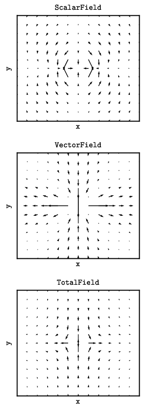
We solve the equations for and numerically with a standard numerical solver33 3 NDSolve of the Mathematica software package. for ordinary differential equations and for initial conditions chosen so that the string passes close to a test particle in the direction (at a distance ), starting at a distance far away and moving past the particle in the direction again to a distance such that (the near-by limit). We find that the net acceleration in the direction cancels roughly out, while the net effect in the direction, in particular the velocity kick, agrees with the predicted value [1]
| (37) |
Our numerical result for the effect of a GUT string with travelling at past a particle with is
| (38) |
and the agreement can be improved nearly arbitrarily as . We also inserted the modified acceleration equations (35) and (36) into the public N-body code Gadget-2 [36] and found that the N-body code result agrees with the result from the numerical solver to machine accuracy as long as as we resolve the dynamical time of the particle string interaction in the N-body code. This can be tuned to any precision when looking at the effect on single particles (however, this may be a problem to be solved when doing large scale N-body simulations where a general small limit on the maximum timestep is too expensive). We conclude that our formalism and simulation set-up reproduces the standard results in non-expanding space time accurately.
Details of the particle motion (from the N-body code) are shown in Fig. 3. The acceleration in the direction (along the motion of the string, left panels of the figure) averages to zero, so that there is no net velocity left after the string has passed, and only a small overall displacement. It is however remarkable how the scalar and vector parts combine to a smooth overall motion, which is best visible in the middle panel on the left for the velocity in the direction. In the direction (perpendicular to the string motion) we can see the particle receiving the above-mentioned velocity kick. The contribution from the vector part is small and mostly serves to render the kick more step-like.
When looking in more detail at the late-time impact of the scalar and vector parts of the acceleration field, we find that in the near-by limit the vector part does not contribute significantly to the final velocity, see Fig. 4. However, this is due not least to the special case that we consider, where a long, straight string moves on a straight trajectory past a particle. In reality we will be dealing with a string network, in which case strings are not straight, and they move on curved trajectories. In this case we would not expect to satisfy the near-by limit at all times. In this situation the vector part can contribute at a level comparable to the scalar part.


V N-body results with a moving straight string in expanding space-time
We now turn to the cosmologically more relevant case of uniformly expanding space-time. Specifically, we consider an infinite, straight string moving through an initially homogeneous distribution of particles expanding with the Hubble flow and follow the subsequent evolution of those particles. We present here our leading order results and put our higher order calculations into Appendix C.
We find that the energy momentum tensor of the Nambu Goto string in a FLRW space-time is the same as in Minkowski space-time, except for a factor . This factor cancels out when calculating which is used in the Einstein equations (12,13) so that
| (39) |
The vector and the tensor perturbations stay the same, while the scalar potentials become
| (40) |
| (41) |
where .
| (42) |
While the logarithmically divergent contributions at small and large distances in the metric perturbations (29) and (30) did not enter the equations of motion in Minkowski space-time, we now have to deal with the term . We discuss in Appendix A the (unphysical) origin of these divergences and how we regularise them, and we show that they do not influence the results.
The EOM become
| (43) |
| (44) |
When the string passes near a particle, this particle will be imparted a velocity towards the string (the velocity kick discussed above). In physical coordinates with the origin fixed to a point on the string trajectory, however, the particle is still following the Hubble flow until the recession velocity drops below the velocity due to the string passage. The particle will then start to move towards the region through which the string has passed, and we expect that the particles will form a wake behind the string once they reach this region. Quantitatively, we can compare the particle motion w.r.t. the axis of symmetry and the turn-around radius at which the particle motion decouples from the Hubble flow to the calculation based on the Zel’dovich approximation in [1]: The physical particle position is given by
| (45) |
where is the initial particle position and describes its displacement,
| (46) |
(at late times, , only the first term in the square brackets is relevant). We set for and for as the velocity kick is always towards the string, is the predicted velocity kick (37) and , are the time and scale factor at which the predicted velocity kick occurs (i.e. the moment when for a particular particle). From the particle trajectory it is easy to compute the turn-around radius, since at turn-around . One finds that for the particle that turns around at time ,
| (47) |
For testing purposes our simulation starts with a homogeneous distribution of particles on an uniform grid in a box size of . We start at redshift . The string is initially at position . We evolve the simulation with the string until it reaches position at which point we turn it off. Thereafter we evolve only the particles and since we use these simulations to test the implementation of our formalism, we use the expansion rate of a matter dominated universe throughout as the approximation above was derived under this assumption.

Our results and comparison to the analytically-predicted trajectories and turnaround radii are shown in Figure 5. The numerically calculated particle trajectories initially follow closely the analytical predictions. Eventually the numerical results diverge from the analytical ones due to the fact that in the simulation the velocity kick for particles that are further away from the axis of symmetry is smaller than the analytically predicted velocity kick, which is derived assuming that the string that came from and went to infinity.
VI Conclusion and Outlook
In this paper we set up the formalism needed to include topological defects and other sources of weak gravitational fields in N-body simulations. For this purpose, we have derived the equations of motion of massive particles (Equation 16) in a perturbed background. We find that both scalar and vector (gravito-magnetic) perturbations contribute significantly to leading order, .
Tensor perturbations on the other hand do not contribute to leading order, and their contribution to the acceleration is suppressed by one power of (we investigate the impact of the tensor perturbations in Appendix C).
To test and illustrate the equations, we have applied the leading order result (Equation 17) to the well known example of a straight string. We have recovered the expected velocity kick in the limit where the string passes very close to a particle (relative to the distance that the string travels) and we have found that the vector contribution to the final particle motion is sub-dominant. Furthermore we have recovered the turn-around radii in FLRW spacetime.
Note that this is the first full numerical calculation (to first order in ) where the velocity kick was not simply taken as an initial condition.
Our results can be used for calculating the effect of any sources of weak gravitational fields on non relativistic and on relativistic particles. The focus of our continuing work is on doing large scale N-body simulations and calculating the effect of Abelian Higgs cosmic string networks [37] on large scale structures.
Acknowledgements.
We thank Volker Springel for his N-body code Gadget2 [36]. This work was partially funded by a STFC DPhil studentship. M.O. and M.K. acknowledge financial support by the Swiss National Science Foundation. I.T.I. was supported by the Southeast Physics Network (SEPnet). We acknowledge support from the Science and Technology Facilities Council [grant numbers ST/F002858/1, ST/I000976/1].Appendix A Unphysical term
An additional complication in the case of expanding background compared to the Minkowski space-time is evidenced by equation (17). Since now , there is an additional force term proportional to , which is logarithmically-diverging with distance to the string. This unphysical divergence arises because of the idealised nature of the infinitely long, straight Nambu-Goto string: A string of finite thickness would regularise automatically the divergence for small radii, , while the divergence at large distances, is due to the assumed infinite length of the string. This is analogous to the logarithmic divergence exhibited by the electrostatic potential of an infinite line charge. The divergence at small separations is not an issue here because the physical thickness of a realistic string is very small compared to the typical inter-particle separation in a cosmological N-body simulation. However, we would expect that in a cosmological setting the size of the causal horizon would provide an upper cutoff, above which strings are not formed.
For this reason we have decided to set to horizon size and such that for all particles initially (we place the string initially at a distance from the box and since , initially for all particles).
This term only affects the motion in the direction, and hence it does not influence our results and comparison to the analytical predictions discussed above.
Appendix B Tensor Perturbations
To get the contribution due to the tensor term we solve the differential equation (12) for the tensor source
| (48) |
where
For a general tensor sorce, the numerical method involves solving the differential equation on each grid point in Fourier space, and then numerically inverse Fourier transforming the resulting which is used in the equation of motion.
However, in the case of the Nambu Goto string we directly solve the differential equation analytically for modes that are well inside the horizon, ie . Dropping the friction term (note that this term also disappears in Minkowskian spacetime) we can rewrite it to read
| (49) |
where we define and use to make the time dependence explicit. Hence
| (50) |
where is a solution to the homogeneous equation , determined by the initial conditions.
Equation (50) represents the tensor part of the boosted static gravitational field of the string when . Hence we arrive at our solution
| (51) | |||||
| (52) |
We also find the analytic solution to the full differential equation (12) for the tensor source (48)
| (53) | |||||
However, we find that when comparing over our ranges and scales of interest (, ) for which .
Appendix C Equations of motion to first order in the velocity
The equation of motion to first order in the particle velocities, in physical time, is
| (54) | |||||
We find that all the contributions to first order in the particle velocity are significantly smaller (suppressed by one power of ) and they hence do not influence the result (see Figure 6). For completeness we list here all the additional first order analytical results.
The first order scalar contributions are given by
| (55) | |||||
The first order vector contributions are given by
| (56) |
| (57) |
| (58) |
| (59) |
Note that the first two of these terms come from the term.
The first order tensor contributions are given by inverse Fourier transforming Equation (52)
| (60) | |||||
| (61) | |||||
| (62) | |||||
| (63) |
Finally, note that in equation (16) there are further terms of order and which will be smaller yet.

References
- [1] A. Vilenkin and E. P. S. Shellard, Cosmic Strings And Other Topological Defects (Cambridge Univ. Press, 1994).
- [2] M. Hindmarsh and T. Kibble, Rept.Prog.Phys. 58, 477 (1995), eprint hep-ph/9411342.
- [3] M. Sakellariadou, Lect.Notes Phys. 718, 247 (2007), eprint hep-th/0602276.
- [4] E. J. Copeland and T. Kibble, Proc.Roy.Soc.Lond. A466, 623 (2010), eprint 0911.1345.
- [5] J. Yokoyama, Phys.Rev.Lett. 63, 712 (1989).
- [6] A. D. Linde, Phys.Rev. D49, 748 (1994), eprint astro-ph/9307002.
- [7] E. J. Copeland, A. R. Liddle, D. H. Lyth, E. D. Stewart, and D. Wands, Phys.Rev. D49, 6410 (1994), eprint astro-ph/9401011.
- [8] M. Sakellariadou, Lect.Notes Phys. 738, 359 (2008), eprint hep-th/0702003.
- [9] R. Jeannerot, J. Rocher, and M. Sakellariadou, Phys.Rev. D68, 103514 (2003), eprint hep-ph/0308134.
- [10] N. Bevis, M. Hindmarsh, and M. Kunz, Phys.Rev. D70, 043508 (2004), eprint astro-ph/0403029.
- [11] N. Bevis, M. Hindmarsh, M. Kunz, and J. Urrestilla, Phys.Rev.Lett. 100, 021301 (2008), eprint astro-ph/0702223.
- [12] J. Urrestilla, N. Bevis, M. Hindmarsh, M. Kunz, and A. R. Liddle, JCAP 0807, 010 (2008), eprint 0711.1842.
- [13] M. Hindmarsh, Prog.Theor.Phys.Suppl. 190, 197 (2011), eprint 1106.0391.
- [14] R. A. Battye, B. Garbrecht, and A. Moss, JCAP 0609, 007 (2006), eprint astro-ph/0607339.
- [15] R. Battye, B. Garbrecht, and A. Moss, Phys.Rev. D81, 123512 (2010), eprint 1001.0769.
- [16] R. Battye and A. Moss, Phys.Rev. D82, 023521 (2010), eprint 1005.0479.
- [17] M. Landriau and E. Shellard, Phys.Rev. D67, 103512 (2003), eprint astro-ph/0208540.
- [18] B. A. Reid, W. J. Percival, D. J. Eisenstein, L. Verde, D. N. Spergel, et al., Mon.Not.Roy.Astron.Soc. 404, 60 (2010), eprint 0907.1659.
- [19] D. H. Lyth and A. R. Liddle (2009).
- [20] A. Albrecht and A. Stebbins, Phys. Rev. Lett. 68, 2121 (1992).
- [21] M. Hindmarsh, C. Ringeval, and T. Suyama, Phys.Rev. D80, 083501 (2009a), eprint 0908.0432.
- [22] M. Hindmarsh, C. Ringeval, and T. Suyama, Phys.Rev. D81, 063505 (2010), eprint 0911.1241.
- [23] C. Ringeval, Adv.Astron. 2010, 380507 (2010), * Temporary entry *, eprint 1005.4842.
- [24] A. Stebbins, S. Veeraraghavan, J. Silk, R. Brandenberger, and N. Turok, Astrophys. J. 322, 1 (1987).
- [25] T. Hara and S. Miyoshi, Progress of Theoretical Physics 77, 1152 (1987), URL http://ptp.ipap.jp/link?PTP/77/1152/.
- [26] A. Sornborger, R. Brandenberger, B. Fryxell, and K. Olson, Astrophys. J. 482, 22 (1997), eprint arXiv:astro-ph/9608020.
- [27] A. Sornborger, Phys. Rev. D 56, 6139 (1997), eprint arXiv:astro-ph/9702038.
- [28] J. Silk and A. Vilenkin, Phys. Rev. Lett. 53, 1700 (1984).
- [29] M. Hindmarsh, S. Stuckey, and N. Bevis, Phys.Rev. D79, 123504 (2009b), eprint 0812.1929.
- [30] J. Moore, E. Shellard, and C. Martins, Phys.Rev. D65, 023503 (2002), eprint hep-ph/0107171.
- [31] H. Kodama and M. Sasaki, Prog.Theor.Phys.Suppl. 78, 1 (1984).
- [32] V. F. Mukhanov, H. Feldman, and R. H. Brandenberger, Phys.Rept. 215, 203 (1992).
- [33] C.-P. Ma and E. Bertschinger, Astrophys.J. 455, 7 (1995), eprint astro-ph/9506072.
- [34] R. Durrer, Fund.Cosmic Phys. 15, 209 (1994), eprint arXiv:astro-ph/9311041.
- [35] R. Durrer, M. Kunz, and A. Melchiorri, Phys. Rept. 364, 1 (2002), eprint astro-ph/0110348.
- [36] V. Springel, Mon. Not. Roy. Astron. Soc. 364, 1105 (2005), eprint astro-ph/0505010.
- [37] N. Bevis, M. Hindmarsh, M. Kunz, and J. Urrestilla, Phys. Rev. D 75, 065015 (2007), eprint arXiv:astro-ph/0605018.