CERN-PH-TH/2011-150
LCTS/2011-07
25th July 2011
PDF dependence of Higgs cross sections at the Tevatron and LHC: response to recent criticism
Abstract
We respond to some criticism questioning the validity of the current Standard Model Higgs exclusion limits at the Tevatron, due to the significant dependence of the dominant production cross section from gluon–gluon fusion on the choice of parton distribution functions (PDFs) and the strong coupling (). We demonstrate the ability of the Tevatron jet data to discriminate between different high- gluon distributions, performing a detailed quantitative comparison to show that fits not explicitly including these data fail to give a good description. In this context we emphasise the importance of the consistent treatment of luminosity uncertainties. We comment on the values of obtained from fitting deep-inelastic scattering data, particularly the fixed-target NMC data, and we show that jet data are needed for stability. We conclude that the Higgs cross-section uncertainties due to PDFs and currently used by the Tevatron and LHC experiments are not significantly underestimated, contrary to some recent claims.
Keywords
Higgs Physics, Jets, Deep Inelastic Scattering, Hadronic Colliders1 Introduction
Discovery or exclusion of the Standard Model Higgs boson () at the Tevatron and Large Hadron Collider (LHC) requires precise knowledge of the theoretical cross section; see, for example, refs. [1, 2, 3], and references therein. Cross-section predictions for the dominant production channel of gluon–gluon fusion () are strongly dependent on both the gluon distribution in the proton and the strong coupling , which enters squared at leading-order (LO) with sizeable next-to-leading order (NLO) and next-to-next-to-leading order (NNLO) corrections. In particular, the Tevatron Higgs analysis [4, 5], with current exclusion at 95% confidence-level (C.L.) for a Standard Model Higgs boson mass GeV [5], requires knowledge of the gluon distribution at relatively large momentum fractions where constraints from data on deep-inelastic scattering (DIS) or Drell–Yan production are fairly weak. In this paper, which accompanies a separate paper [6], we respond to several (related) issues which have been raised in recent months [7, 8, 9, 10, 11, 12], particularly regarding the use of parton distribution functions (PDFs) determined from limited data sets in making predictions for the Tevatron (and LHC) Higgs cross sections, as alternatives to the most common choice of the MSTW 2008 PDFs [13] used in the Tevatron [4, 5] and LHC [3] Higgs analyses.
First in section 2 we demonstrate explicitly how the cross sections depend on the Standard Model Higgs boson mass , the gluon–gluon luminosity function and the choice of , by comparing predictions obtained using PDFs (and values) from various different PDF fitting groups. In section 3 we present a detailed quantitative comparison of the quality of the description of Tevatron jet data using different PDF sets. The MSTW 2008 analysis [13] is the only current NNLO PDF fit which includes the Tevatron jet data, providing the only direct constraint on the high- gluon distribution. In section 4 we examine the different values of the strong coupling used by the different PDF groups, particularly those values mainly extracted from DIS data, and we look at the constraints arising from different sources. In section 5 we respond to recent claims [11] that the theoretical treatment of the longitudinal structure function for the NMC data [14] can explain the bulk of the difference between predictions for Higgs cross sections calculated using either the MSTW08 [13] or ABKM09 [15] PDFs. Finally we conclude in section 6 that MSTW08 is presently the only fully reliable PDF set for calculating Higgs cross sections at NNLO, particularly if sensitive to the high- gluon distribution, and that the recent exclusion bounds [4, 5] obtained by the Tevatron experiments are robust based upon this choice.
2 Dependence of Higgs cross sections on PDFs and
2.1 Dependence on Higgs mass
(a)

(b)

(c)

(d)

We show the NLO and NNLO total cross sections () versus the Standard Model Higgs boson mass in figure 1 at the Tevatron (centre-of-mass energy, TeV) and the LHC ( TeV) for different PDF sets and a fixed scale choice of , calculated with settings given in section 4.2 of ref. [6]. At NLO [16], we use the corresponding NLO PDFs (and values) from MSTW08 [13], CTEQ6.6 [17], CT10 [18] and NNPDF2.1 [19], all of which are fully global fits to HERA and fixed-target DIS data, fixed-target Drell–Yan production, and Tevatron data on vector boson and jet production. At NNLO [20], we use the corresponding NNLO PDFs (and values) from MSTW08 [13], ABKM09 [15], JR09 [21, 22] and HERAPDF1.0 [23], where in the last case no uncertainty PDF sets are provided and the two curves correspond to and , with the larger value giving the larger Higgs cross section. For the other PDF sets, we compute the “PDF+” uncertainty at 68% C.L. according to the recommended prescription of each group, summarised in ref. [6]. The data sets included in the MSTW08 fit at NNLO are the same as at NLO, with the omission of HERA data on jet production, while the ABKM09 and JR09 fits only include DIS and fixed-target Drell–Yan data. The HERAPDF1.0 fit only includes combined HERA I inclusive DIS data, while the other NNLO fits (MSTW08, ABKM09, JR09) instead include the older separate data from H1 and ZEUS. However, including the combined HERA I data [23] in a variant of the MSTW08 fit was found to have little effect on predictions for Higgs cross sections [24]. The NNPDF fits parameterise the starting distributions at GeV2 as neural networks, whereas other groups all use the more traditional approach of parameterising the input PDFs as some functional form in , each with a number of free parameters, which varies significantly between groups. Contrary to the “standard” input parameterisation at GeV2, the JR09 set uses a “dynamical” parameterisation of valence-like input distributions at an optimally chosen GeV2, which gives a slightly worse fit quality and lower values than the corresponding “standard” parameterisation, but is nevertheless favoured by the JR09 authors. More details on differences between PDF sets are given in section 2 of ref. [6]; see also the descriptions in refs. [25, 26, 27].
The size of the higher-order corrections to the total cross sections is substantial. Taking the appropriate MSTW08 PDFs and values consistently at each perturbative order for with GeV, then the NLO/LO ratio is 2.1 (Tevatron) or 1.9 (LHC), the NNLO/LO ratio is 2.7 (Tevatron) or 2.4 (LHC), and so the NNLO/NLO ratio is 1.3 (Tevatron and LHC). The perturbative series is therefore slowly convergent, mandating the use of (at least) NNLO calculations together with the corresponding NNLO PDFs and values. The convergence can be improved by using a scale choice , which mimics the effect of soft-gluon resummation. However, the goal of this paper is to study only the PDF and dependence of the cross sections, and we do not aim to come up with a single “best” prediction together with a complete evaluation of all sources of theoretical uncertainty. We do not consider, for example, optimal (factorisation and renormalisation) scale choices and variations, electroweak corrections, the effect of threshold resummation, -enhanced terms, use of a finite top-quark mass in the calculation of higher-order corrections, bottom-quark loop contributions, etc. The PDF and dependence roughly decouples from these other, more refined, aspects of the calculation, and therefore the findings regarding PDFs and reported here will be relevant also for more complete calculations found, for example, in refs. [1, 2] or the recent Handbook of LHC Higgs Cross Sections [3].
(a)

(b)

(c)

(d)

(a)

(b)

(c)

(d)

The ratios of the cross sections with respect to the MSTW08 predictions are shown for the Tevatron in figure 2 and for the LHC in figure 3, where PDF+ uncertainty bands at both 68% and 90% C.L. are plotted. It can be seen that there is generally good agreement between the global fits at NLO. However, at NNLO, the ABKM09 prediction, and the HERAPDF1.0 prediction with the lower value, are well below MSTW08 at the Tevatron, even allowing for the 90% C.L. PDF+ uncertainties, with a significant discrepancy also at the LHC.
Baglio, Djouadi, Ferrag and Godbole (BDFG) [9] have claimed that some publicly available PDFs, specifically the HERAPDF1.0 NNLO set with , can lower the Tevatron Higgs cross section by up to 40% compared to MSTW08 for GeV, requiring more than twice as much Tevatron data to recover the same sensitivity as the 2010 analysis by the Tevatron experiments [4], which used MSTW08 for the central prediction. This is obviously potentially very worrying. However, figure 2(c,d) shows that the lowest cross section occurs not with either of the HERAPDF sets, but with ABKM09, where the central cross section is that of MSTW08 at GeV. The cross-section ratios for ABKM09 and JR09 in figure 2(d) seem close to those in the inset of figure 1 of ref. [9], but we do not reproduce the extreme behaviour of the HERAPDF1.0 sets. Our results are supported by those in ref. [10] where it is also observed that ABKM09 gives lower Higgs cross sections at the Tevatron than the HERAPDF1.0 set with . One obvious difference is the scale choice used in ref. [9] rather than used here and in ref. [10]. However, we have checked that the ratio of cross sections with respect to MSTW08 is largely independent of the different scale choice. The detailed arguments of ref. [9] assume the “worst-case scenario” of a 40% reduction in at GeV from the central value of HERAPDF1.0 with , and therefore the conclusions require modification if there is a mistake in their HERAPDF1.0 calculations.11 1 We thank J. Baglio for confirming that the HERAPDF1.0 curves in figure 1 of ref. [9] were erroneously drawn with , to be corrected in an erratum included in v3 of the preprint version [9]. Nevertheless, even the 25% reduction in at GeV from the central value of ABKM09 is still a problem, as it lies well outside both the MSTW08 PDF+ uncertainty at 90% C.L. used in ref. [4] and the PDF4LHC22 2 The PDF4LHC recommendation [28] is to rescale the MSTW08 NNLO PDF+ uncertainty at 68% C.L. by the ratio of the envelope of the MSTW08 NLO, CTEQ6.6 NLO and NNPDF2.0 NLO predictions, all including PDF+ uncertainties at 68% C.L., to the MSTW08 NLO PDF+ 68% C.L. uncertainty. uncertainty used in ref. [5]. (These two prescriptions for uncertainties give similar results, but the former is clearly much simpler; see section 5 of ref. [6] for more discussion.) We note that in justifying the use of the HERAPDF set, BDFG [9] make the statement: “However, HERAPDF describes well not only the Tevatron jet data but also the , data. Since this is a prediction beyond leading order, it has also the contributions of the gluon included. This gives an indirect test that the gluon densities are predicted in a satisfactory way.” This statement is very misleading: the charge asymmetry and the rapidity distribution at the Tevatron, used as a PDF constraint, are almost insensitive to the gluon distribution, and the statement makes no reference to the quantitative comparison of PDFs to jet data. In the rest of this paper we will present a number of arguments to show that, of all the currently available NNLO PDF sets, only MSTW08 provides a fully reliable estimate of the Higgs cross sections at the Tevatron and LHC.
2.2 Dependence on luminosity
At LO, the PDF dependence of the total cross section is simply given by the gluon–gluon luminosity evaluated at a partonic centre-of-mass energy ,
| (1) |
where is the gluon distribution and .
(a)

(b)

(c)

(d)

In figure 4 we show the gluon–gluon luminosities calculated using different PDF sets and taken as the ratio with respect to the MSTW 2008 value, at centre-of-mass energies corresponding to the (a,b) Tevatron and (c,d) LHC. The relevant values of GeV are indicated, along with the threshold for production at the LHC, with GeV, where this process is predominantly -initiated at the LHC. Indeed, production at the LHC is strongly correlated with production at the Tevatron, with both processes probing the gluon distribution at similar values, as seen from figure 4. We point out in ref. [6] that the current cross-section measurements at the LHC [29, 30] seem to distinctly favour MSTW08 over ABKM09.
The NLO luminosities in figure 4(a,c) are shown for the global fits from MSTW08 [13], CTEQ6.6 [17], CT10 [18] and NNPDF2.1 [19]. The NNLO luminosities in figure 4(b,d) are shown for MSTW08 [13], HERAPDF1.0 [23], ABKM09 [15] and JR09 [21, 22]. The two HERAPDF1.0 NNLO curves shown are for both and , where the latter gives the smaller luminosity at low values and the larger luminosity at high values. The larger value means that less gluon is required at low to fit the scaling violations of HERA data, , therefore more gluon is required at high from the momentum sum rule. Both these effects, larger and more high- gluon, raise the Tevatron Higgs cross section and improve the quality of the description of Tevatron jet data, as we will see in section 3. The NNLO trend between groups is similar to at NLO [6]. There is reasonable agreement for the global fits, but more variation for the other sets, particularly at large , where HERAPDF1.0 and ABKM09 have much softer high- gluon distributions, and this feature has a direct impact on the cross sections, particularly at the Tevatron (see figure 2).
2.3 Dependence on strong coupling
(a)

(b)

The various PDF fitting groups take different approaches to the values of the strong coupling and, for consistency, the same value as used in the fit should be used in subsequent cross-section calculations. The values of , and the corresponding uncertainties, for MSTW08, ABKM09 and GJR08/JR09 are obtained from a simultaneous fit with the PDF parameters. Other groups choose a fixed value, generally close to the world average [31], and for those groups we assume a 1- uncertainty of [26], very similar to the MSTW08 uncertainty. The central values and 1- uncertainties are depicted in figure 5 as the larger symbols and error bars, while the smaller symbols indicate the PDF sets with alternative values of provided by each fitting group. The fitted NLO value is always larger than the corresponding NNLO value in an attempt by the fit to mimic the missing higher-order corrections, which are generally positive. The world average [31], shown in figure 5, combines determinations made at a variety of perturbative orders, but in most cases an increase in the order corresponds to a decrease in the value of obtained.
(a)

(b)

(c)

(d)

(e)

(f)

(a)

(b)

(c)

(d)

(e)

(f)

The cross sections at the Tevatron and LHC start at at LO, with anomalously large higher-order corrections, therefore they are directly sensitive to the value of . Moreover, there is a known correlation between the value of and the gluon distribution, which additionally affects the cross sections. In figures 6 and 7 we show this sensitivity by plotting the Higgs cross sections versus at the Tevatron and LHC for Higgs masses GeV. We plot both NLO and NNLO predictions for a fixed scale choice . The format of the plots is that the markers are centred on the default value and the corresponding predicted cross-section of each group. The horizontal error bars span the uncertainty, the inner vertical error bars span the “PDF only” uncertainty where possible (i.e. not for ABKM09 or GJR08/JR09, where is mixed with the input PDF parameters in the error matrix), and the outer vertical error bars span the PDF+ uncertainty. The effect of the additional uncertainty is sizeable. The dashed lines at NLO or the solid lines at NNLO interpolate the cross-section predictions calculated with the alternative PDF sets provided by each group, represented by the smaller symbols in figure 5. The NNLO plots in figure 7 also show the NLO predictions (open symbols and dashed lines) together with the corresponding NNLO predictions (closed symbols and solid lines) to explicitly demonstrate how the size of the NNLO corrections depends on both the choice and the PDF choice. It is apparent from the plots that at least part of the MSTW08/ABKM09 discrepancy for Higgs cross sections is due to using quite different values of at NNLO, specifically for ABKM09 [15] compared to for MSTW08 [13, 32]. Comparing cross-section predictions at the same value of would reduce the MSTW08/ABKM09 discrepancy at the LHC, but there would still be a significant discrepancy at the Tevatron (see also the later table 5 in section 5).
2.4 Theoretical uncertainties on
In ref. [32] we gave a prescription for calculating the “PDF+” uncertainty on an observable such as a hadronic cross section, due to only experimental errors on the data fitted. An estimate of the theoretical uncertainty on was given as at NLO and at most at NNLO, where these values should be interpreted as roughly 1- (68% C.L.). However, this additional uncertainty was not recommended to be propagated to the “PDF+” uncertainty on cross sections, in the same way that theoretical errors on PDFs are not generally provided and propagated to uncertainties on cross sections. It was intended simply to be an estimate of how much the value of might change if extracted at even higher orders. It has subsequently been proposed (by Baglio and Djouadi) to include the theoretical uncertainty on in the cross-section calculation for the process at the Tevatron [7] and LHC [8], which somewhat reduces the apparent inconsistency between MSTW08 and ABKM09 seen in figures 2 and 3.
(a)

(b)

(c)

(d)

In figure 8 we show the effect of adding in quadrature an additional theoretical uncertainty on to the 90% C.L. MSTW08 PDF+ uncertainty for the cross sections at both the Tevatron and LHC, at both NLO and NNLO, plotted as a function of the Higgs mass .33 3 We calculate the cross sections evaluated with at NLO and at NNLO, to determine the variation due to the additional theoretical uncertainty on at 68% C.L., then we scale this uncertainty by 1.64485 to get the 90% C.L. theoretical uncertainty. If a similar theoretical uncertainty on was also added to the ABKM09 uncertainty band, which includes only experimental uncertainties, then the MSTW09 and ABKM09 uncertainty bands would overlap at the Tevatron, at least in the range shown here. However, even if the additional uncertainty is applied in this manner, it is misleading to claim that it leads to more of an agreement in the predictions obtained using the two PDF sets, since variations of cross sections with are very highly correlated between different PDF sets. We will see in the rest of this paper that differences between groups in values, gluon distributions and Higgs cross sections are largely due to the selection of data fitted, and it is not the case that the discrepancies should be attributed to unaccounted theoretical uncertainties.
3 Constraints from jet production at the Tevatron
Here we present a quantitative study of the description of the Tevatron Run II inclusive jet data [33, 34, 35] and dijet data [36] by different PDF sets. The goal is to compare the description of Tevatron jet data in a similar manner to the benchmark cross-section study of ref. [6], i.e. we use the same code and settings for all NLO and NNLO PDF sets (with the correct value for each set) to ensure that observed differences are only due to the PDF choice rather than any other factor. We do not consider the less reliable Tevatron Run I data, which prefer a much harder high- gluon distribution [13], and are obtained using less sophisticated jet algorithms. The three data sets on inclusive jet production from the Tevatron Run II [33, 34, 35] were all found to be compatible [13]. The MSTW 2008 analysis [13] included the CDF Run II inclusive jet data using the jet algorithm [33] and the DØ Run II inclusive jet data using a cone jet algorithm [35]. Consistency was checked with the CDF Run II inclusive jet data using the cone-based Midpoint jet algorithm [34], but this data set was not included in the final MSTW08 fit, since it is essentially the same measurement (using 1.13 fb-1) as ref. [33] (using 1.0 fb-1), differing mainly by the choice of jet algorithm. The jet algorithm is theoretically preferred due to its property of infrared safety, and the corresponding CDF Run II data [33] was already published and implemented in the MSTW08 analysis by the time the CDF Run II Midpoint data [34] appeared. The DØ Run II inclusive jet data [35] and dijet data [36], both defined using a cone jet algorithm, are also measured from essentially the same 0.7 fb-1 of data, differing mainly by the kinematic binning, so as with the two CDF data sets it would be double-counting to include both in the same PDF extraction. We will concentrate on the inclusive jet data (section 3.2), but we will also make a first quantitative comparison to the more recent DØ dijet data (section 3.3). However, first in section 3.1 we precisely define the goodness-of-fit measure used for the comparison of data and theory.
One obvious problem is that the complete NNLO partonic cross section () for inclusive jet production is currently unknown, and needs to be approximated with the NLO supplemented by 2-loop threshold corrections [37], while even these 2-loop threshold corrections are unavailable for the dijet cross section. We calculate jet cross sections using fastnlo [38] (based on nlojet++ [39, 40]), which includes these 2-loop threshold corrections. Following the usual way of estimating theoretical uncertainties due to unknown higher-order corrections, we take different scale choices as some indication of the theoretical uncertainty. Smaller scale choices raise the partonic cross section, so favour softer high- gluon distributions [13], and the central was chosen for the final MSTW08 fit [13]. We comment on the scale dependence in section 3.4, we present distributions of pulls and systematic shifts in section 3.5, we briefly discuss other collider data on jet cross sections in section 3.6, then finally we summarise our findings in section 3.7.
3.1 Definition of goodness-of-fit,
It is important to account for correlated systematic uncertainties of the experimental data points. The full correlated error information is accounted for by using a goodness-of-fit () definition given by [41, 42]
| (2) |
where are the theory predictions and
| (3) |
are the data points allowed to shift by the systematic errors in order to give the best fit. Here, labels the individual data points and labels the individual correlated systematic errors. The data points have uncorrelated (statistical and systematic) errors and correlated systematic errors . Minimising the in eq. (2) with respect to the systematic shifts gives the analytic result that [41, 42]
| (4) |
where
| (5) |
and is the Kronecker delta. Therefore, the optimal shifts of the data points by the systematic errors, eq. (3), are solved for analytically. Here we use the same notation44 4 We note a typo, already pointed out in ref. [43], in the formula for in eq. (40) of ref. [13] where should appear squared. This typo is corrected in eq. (5) above. as in the MSTW08 paper [13]. We treat the luminosity uncertainty as any other correlated systematic. However, we find that the relevant systematic shift – for some PDF sets with soft high- gluon distributions (e.g. ABKM09 and HERAPDF1.0), which is clearly completely unreasonable, as it means that the data points are normalised downwards by 3–5 times the nominal luminosity uncertainty (around 6% for both CDF and DØ). The penalty term will contribute only 9–25 units to the total given by eq. (2), which can therefore still lead to reasonably low overall values (see appendix A for details).
It is the usual situation at collider experiments that the luminosity determination is common to all cross sections measured from a given data set (see, for example, refs. [44, 45]), so the requirement of a single common luminosity is mandatory when fitting multiple measurements taken during a single running period.
(a)

(b)

In figure 9 we compare NNLO predictions for the and total cross sections at the Tevatron Run II, calculated in the zero-width approximation with settings described in ref. [6]; see also similar comparisons in ref. [10]. The format of the plots in figure 9 is the same as for the cross sections in section 2.3, i.e. we show the cross-section predictions plotted against . We compare to CDF Run II data on [46] and [47] total cross sections, and to DØ Run II data on the total cross section [48]. The thicker horizontal lines in figure 9 indicate the central value of each experimental measurement, the thinner horizontal lines indicate the statistical and systematic (excluding luminosity) uncertainties added in quadrature, while the shaded regions indicate the total uncertainty obtained by also adding the luminosity uncertainty in quadrature. The plotted CDF measurement with 2.1 fb-1 [47] supersedes the earlier measurement with 72 pb-1 [46], but both measurements are dominated by the (common) luminosity uncertainty. The DØ experiment has not published any dedicated and total cross-section measurements from Run II at the Tevatron. The DØ total cross section shown in figure 9(b) was obtained as part of the +jet measurement [48]. The CDF measurement [47] is defined as the cross section in an invariant mass range GeV, while the DØ measurement [48] is defined as the cross section in an invariant mass range GeV. We have therefore multiplied the CDF and DØ data by factors of 1.006 and 1.004, respectively, derived using the vrap code [49] at NNLO with MSTW08 PDFs, to correct to the -only cross section with . We note from figure 9 that the MSTW08, ABKM09 and JR09 NNLO predictions for the and total cross sections at the Tevatron are in good agreement with the CDF data [46, 47], and lie around 1- above the DØ data [48]. In the MSTW08 fit [13], the luminosity shift for the CDF jet data was correctly tied to be the same as for the more-constraining CDF rapidity distribution, [47], which therefore effectively acted as a luminosity monitor. The optimal CDF normalisation in the MSTW08 NNLO fit [13] was found to be very close to the nominal value, therefore it is not surprising that the CDF total cross section is well described in figure 9(b). The DØ experiment instead measured the rapidity shape distribution, [50], also included in the MSTW08 fit, which is one reason why the DØ jet data were found to be less constraining than the CDF jet data; see ref. [32]. The optimal DØ normalisation in the MSTW08 NNLO fit [13], determined only from jet data, was around 1- above the nominal value, consistent with the DØ total cross section shown in figure 9(b). If the Tevatron jet data were normalised downwards by 20–30% (i.e. 3–5 times the luminosity uncertainty), the Tevatron and total cross sections would need to normalised downwards by the same amount, resulting in complete disagreement with all theory predictions shown in figure 9. This example illustrates the utility of simultaneously fitting and cross sections together with jet cross sections at the Tevatron (and LHC). The luminosity shifts, common to both data sets, are effectively determined by the more precise and cross sections. The luminosity uncertainty is then effectively removed from the jet cross sections, thereby allowing the jet data to provide a tighter constraint on the gluon distribution (and ).
To avoid these completely unrealistic luminosity shifts, –, without going into the complication of simultaneously including and cross sections in the computation, we will calculate the values for the Tevatron jet data using eq. (2), but with the simple restriction that the relevant systematic shift . More practically, this means that if for any particular PDF set, we fix at and reevaluate eq. (2) with the luminosity removed from the list of correlated systematics. However, we note from figure 9 that the ABKM09 predictions are slightly above the central value of the CDF and data, and the HERAPDF1.0 predictions are higher by around 1-, while both ABKM09 and HERAPDF1.0 lie above the 1- limit of the DØ data. Allowing luminosity shifts downwards by even 1- is therefore distinctly generous, particularly for HERAPDF1.0, and upwards luminosity shifts would bring the ABKM09 and HERAPDF1.0 predictions into better agreement with the CDF and data, and especially the DØ data. Therefore, it should be understood that the values quoted in the tables we will present in section 3.2 and 3.3 are rather optimistic for ABKM09 and HERAPDF1.0, and more realistic constraints in the luminosity shifts would result in even worse values.
The form of eq. (2) is slightly different from the treatment of normalisation uncertainties adopted in eq. (38) of the MSTW08 paper [13], but is the form used, for example, in the CT10 analysis [18]. Rescaling only the central value of the data in eq. (2), but not the uncertainties, leads to so-called “d’Agostini bias” [51, 52]. However, since we are only comparing and not fitting PDFs, we use the simpler form of eq. (2) which has the major advantage that all shifts can be solved for analytically. A more sophisticated approach to the treatment of normalisation uncertainties may somewhat lessen the preference of some PDF sets for large downwards luminosity shifts, but should not affect our main conclusions. The normalisation uncertainties were treated as multiplicative rather than additive in the MSTW08 fit [13], i.e. the uncertainties were correctly rescaled to reduce bias. Moreover, large normalisation shifts for any experiment were discouraged through use of a quartic penalty term rather than the usual quadratic penalty term in eq. (2). These small differences in definition mean that the MSTW08 values we quote here will be slightly different from the values quoted in ref. [13].
Even considering the constraint on the CDF and DØ luminosities from the comparison to the weak boson cross sections (see figure 9), it might be considered that imposing is too restrictive if the luminosity uncertainty is assumed to be Gaussian. However, as another reason for limiting the luminosity shifts to some extent, we note that it has been claimed (see section 6.7.4 on “Normalizations”, pg. 170” in [53]) that, for many experiments, quoted normalisation uncertainties represent the limits of a box-shaped distribution rather than the standard deviation of a Gaussian distribution. This was one motivation for the more severe quartic penalty term for normalisation uncertainties in the MSTW08 analysis; see discussion in section 5.2.1 of ref. [13]. Nevertheless, if we instead impose rather than , then the change in the values for the most relevant ABKM09 NNLO PDF set with is for the {CDF [33], CDF Midpoint [34], DØ inclusive [35], DØ dijet [36]} data, respectively, so there is not a significant improvement in the values. However, as discussed above, our main argument does not rely on the precise form of the uncertainty on the luminosity determination, but that we can use the and cross sections as a luminosity monitor, where the predictions have small theoretical uncertainties, effectively providing an accurate luminosity determination independently of the CDF and DØ values. Combining these arguments, we consider allowing luminosity shifts downwards by more than 1- to be excessively generous.
There is a clear trade-off between the systematic shifts and the parameters of the gluon distribution. Deficiencies in the theory calculation can be masked to some extent by large systematic shifts, therefore it is important to check that the optimal values are not unreasonable. This is straightforward when using a definition like eq. (2), but is more difficult using an equivalent form written in terms of the experimental covariance matrix,
| (6) |
Then eq. (2) is equivalent [41] to the more traditional form written in terms of the inverse of the experimental covariance matrix:
| (7) |
as used by the ABKM and NNPDF fitting groups. More precisely, NNPDF use a refinement to treat normalisation errors as multiplicative [52], while Alekhin (ABKM) treats all correlated systematic errors as multiplicative [54, 55].
3.2 Inclusive jet production
| NLO PDF (with NLO ) | |||
|---|---|---|---|
| MRST04 | 1.06 (0.59) | 0.94 (0.31) | 0.84 (0.31) |
| MSTW08 | 0.75 (0.30) | 0.68 (0.28) | 0.91 (0.84) |
| CTEQ6.6 | 1.25 (0.14) | 1.66 (0.20) | 2.38 (0.84) |
| CT10 | 1.03 (0.13) | 1.20 (0.19) | 1.81 (0.84) |
| NNPDF2.1 | 0.74 (0.29) | 0.82 (0.25) | 1.23 (0.69) |
| HERAPDF1.0 | 2.43 (0.39) | 3.26 (0.66) | 4.03 (1.67) |
| HERAPDF1.5 | 2.26 (0.40) | 3.05 (0.66) | 3.80 (1.66) |
| ABKM09 | 1.62 (0.52) | 2.21 (0.85) | 3.26 (2.10) |
| GJR08 | 1.36 (0.23) | 0.94 (0.13) | 0.79 (0.36) |
| NNLO PDF (with NLO+2-loop ) | |||
| MRST06 | 2.96 (1.24) | 1.21 (1.18) | 1.03 (0.84) |
| MSTW08 | 1.39 (0.42) | 0.69 (0.44) | 0.97 (0.48) |
| HERAPDF1.0, | 2.64 (0.36) | 2.15 (0.36) | 2.20 (0.46) |
| HERAPDF1.0, | 2.24 (0.35) | 1.17 (0.32) | 1.23 (0.31) |
| ABKM09 | 2.55 (0.82) | 2.76 (0.89) | 3.41 (1.17) |
| JR09 | 0.75 (0.37) | 1.26 (0.41) | 2.21 (0.49) |
| NLO PDF (with NLO ) | |||
|---|---|---|---|
| MRST04 | 2.14 (1.42) | 2.01 (0.54) | 1.57 (0.26) |
| MSTW08 | 1.52 (0.61) | 1.40 (0.27) | 1.16 (0.73) |
| CTEQ6.6 | 1.93 (0.41) | 1.98 (0.21) | 1.78 (0.78) |
| CT10 | 1.75 (0.38) | 1.69 (0.19) | 1.50 (0.76) |
| NNPDF2.1 | 1.69 (0.60) | 1.56 (0.25) | 1.44 (0.60) |
| HERAPDF1.0 | 2.61 (0.23) | 2.73 (0.49) | 2.53 (1.58) |
| HERAPDF1.5 | 2.48 (0.24) | 2.60 (0.49) | 2.44 (1.57) |
| ABKM09 | 1.56 (0.26) | 1.68 (0.65) | 1.69 (2.01) |
| GJR08 | 2.11 (0.71) | 1.75 (0.24) | 1.52 (0.31) |
| NNLO PDF (with NLO+2-loop ) | |||
| MRST06 | 2.83 (2.25) | 2.08 (1.56) | 2.11 (0.86) |
| MSTW08 | 1.67 (0.62) | 1.39 (0.43) | 1.62 (0.37) |
| HERAPDF1.0, | 2.20 (0.25) | 2.06 (0.27) | 2.19 (0.40) |
| HERAPDF1.0, | 2.08 (0.55) | 1.76 (0.33) | 1.99 (0.23) |
| ABKM09 | 1.70 (0.50) | 1.94 (0.71) | 2.26 (1.12) |
| JR09 | 1.57 (0.41) | 2.05 (0.36) | 2.82 (0.39) |
| NLO PDF (with NLO ) | |||
|---|---|---|---|
| MRST04 | 1.86 (2.89) | 1.34 (0.96) | 1.11 (0.30) |
| MSTW08 | 1.45 (0.89) | 1.08 (0.20) | 1.05 (1.22) |
| CTEQ6.6 | 1.62 (1.15) | 1.56 (0.59) | 1.61 (1.35) |
| CT10 | 1.39 (0.88) | 1.26 (0.37) | 1.32 (1.29) |
| NNPDF2.1 | 1.41 (0.87) | 1.29 (0.20) | 1.22 (0.96) |
| HERAPDF1.0 | 1.73 (0.27) | 1.84 (0.74) | 1.83 (2.79) |
| HERAPDF1.5 | 1.78 (0.29) | 1.87 (0.75) | 1.84 (2.81) |
| ABKM09 | 1.39 (0.35) | 1.43 (1.07) | 1.63 (3.66) |
| GJR08 | 1.90 (1.46) | 1.34 (0.45) | 1.03 (0.51) |
| NNLO PDF (with NLO+2-loop ) | |||
| MRST06 | 3.19 (5.00) | 1.77 (3.22) | 1.25 (1.50) |
| MSTW08 | 1.95 (0.90) | 1.23 (0.44) | 1.08 (0.35) |
| HERAPDF1.0, | 2.11 (0.37) | 1.68 (0.35) | 1.41 (0.63) |
| HERAPDF1.0, | 2.28 (0.95) | 1.50 (0.40) | 1.17 (0.21) |
| ABKM09 | 1.68 (0.79) | 1.55 (1.21) | 1.63 (2.04) |
| JR09 | 1.84 (0.47) | 1.61 (0.36) | 1.58 (0.50) |
In tables 1, 2 and 3 we give the per data point, calculated using eq. (2) with the restriction , for the Tevatron Run II data on inclusive jet production [33, 34, 35], for different PDF sets and different scale choices , where is the jet transverse momentum. For NNPDF2.1 the jet cross sections are averaged over 100 replica sets. We give the values defined by simply adding all uncertainties in quadrature, eq. (8), in brackets in the tables. In this case many PDF sets and scale choices give a , so the consistent treatment of correlated uncertainties is vital for the jet data to discriminate. In the table captions we give the values with an identically zero theory prediction, , just to illustrate how the correlated systematic shifts can partially accommodate a clearly inadequate theory prediction. We highlight in bold the values lying inside the 90% C.L. region defined as
| (10) |
where and are the 50th and 90th percentiles of the -distribution with degrees of freedom. (These quantities are defined in detail in section 6.2 of ref. [13].) Here, is defined as the lowest value of all theory predictions in each table, i.e. assumed to be close to the best possible fit, so that the rescaling factor in eq. (10) empirically accounts for any unusual fluctuations preventing the best possible fit having [41]. The 90% C.L. region given in this way is used to determine the PDF uncertainties according to the “dynamical tolerance” prescription introduced in ref. [13], so PDF sets with values far outside this region cannot be considered to give an acceptable description of the data. We consider NLO PDFs from MRST04 [56], MSTW08 [13], CTEQ6.6 [17], CT10 [18], NNPDF2.1 [19], HERAPDF1.0 [23], HERAPDF1.5 (preliminary) [57], ABKM09 [15] and GJR08 [58, 59]. We consider NNLO PDFs from MRST06 [60], MSTW08 [13], HERAPDF1.0 [23], ABKM09 [15] and JR09 [21, 22]. The MRST04 and MRST06 fits only included Tevatron Run I data [61, 62], and were superseded by the MSTW08 fits, but we show the values here just to demonstrate that these older fits do not give a good description of the newer Tevatron Run II data due to their harder high- gluon distribution. The CTEQ6.6 fit includes only the Tevatron Run I data [61, 62], while the CT10 fit includes Run II data [34, 35] in addition to the Run I data [61, 62], contrary to the MSTW08 and NNPDF2.1 fits which include only Run II data [33, 36]. The GJR08 fit included some Run I [62] and Run II [63] data, while the JR09, ABKM09 and HERAPDF fits did not include any Tevatron jet data.
The most constraining data set appears to be the CDF Run II inclusive jet data using the jet algorithm [33] (see table 1) where, other than MSTW08, only NNPDF2.1 gives an acceptable description for , while HERAPDF1.0 and ABKM09 typically give –, and CTEQ6.6/CT10 give better values but still much worse than MSTW08 (and NNPDF2.1). The GJR08/JR09 sets and the HERAPDF1.0 NNLO set with give a reasonable description, at a similar level to CT10, and give predictions for cross sections at the Tevatron which are much closer to the MSTW08 predictions than those from ABKM09 and the HERAPDF1.0 NNLO set with . The same trend is apparent, but to a somewhat lesser extent, for the CDF Run II inclusive jet data using the cone-based Midpoint jet algorithm [34] (see table 2) and the DØ Run II inclusive jet data using a cone jet algorithm [35] (see table 3).
(a)

(b)

(a)

(b)

(a)

(b)

(a)

(b)

In figures 10, 11 and 12 we compare the description of the Tevatron inclusive jet data by the MSTW08 and ABKM09 NNLO PDFs (recall that the latter give the lowest predictions for Tevatron Higgs cross sections) by showing the ratio of data to theory defined in two different ways: (a) first we use the original data points with uncertainties given by adding all errors in quadrature (including luminosity), , with the appropriate value in the plot legends obtained using eq. (8), then (b) we use the shifted data points with uncertainties given by , with the calculated according to eq. (2) and showing the two terms separately in the plot legends. The values for ABKM09 are slightly offset for clarity in the plots. The size of the second penalty term in eq. (2) is some measure of how much the data points are shifted compared to their systematic errors. For example, if the penalty term , then the data points are shifted by, on average, more then 1- for each systematic source . In general, a poor description of data before the systematic shifts leads to a large penalty term and a poor description also after the systematic shifts, although this general statement is not universally true. We note that the shape of the data/theory ratio, both before and after the systematic shifts, looks remarkably similar as a function of both transverse momentum and rapidity in figures 10 and 11. This demonstrates very clearly that the two CDF inclusive jet measurements [33, 34] each contain the same data, but simply analysed in a different way, and the change in analysis method is accounted for extremely well by the change in the theory. Hence, it is not at all surprising that the two data sets can be well described by the same PDF set. Indeed, it was explicitly demonstrated in ref. [34] that the ratios of the cross sections measured with the two jet algorithms were in reasonable agreement with theoretical expectations.
3.3 Dijet production
| NLO PDF (with NLO ) | |||
|---|---|---|---|
| MRST04 | 6.04 (4.93) | 4.54 (2.93) | 2.75 (0.72) |
| MSTW08 | 3.15 (1.63) | 2.25 (0.70) | 1.56 (0.70) |
| CTEQ6.6 | 5.41 (2.22) | 4.85 (1.79) | 3.36 (1.52) |
| CT10 | 4.74 (1.87) | 4.06 (1.32) | 2.70 (1.21) |
| NNPDF2.1 | 2.67 (1.56) | 1.93 (0.66) | 1.47 (0.55) |
| HERAPDF1.0 | 2.05 (0.38) | 2.21 (0.77) | 2.11 (2.28) |
| HERAPDF1.5 | 1.90 (0.34) | 2.00 (0.67) | 1.88 (2.16) |
| ABKM09 | 1.49 (0.33) | 1.41 (0.80) | 1.34 (2.78) |
| GJR08 | 10.7 (3.92) | 7.91 (2.36) | 5.30 (0.66) |
| NNLO PDF (with NLO ) | |||
| MRST06 | 8.06 (5.07) | 6.55 (3.21) | 4.07 (0.96) |
| MSTW08 | 2.38 (0.63) | 1.80 (0.33) | 1.31 (1.24) |
| HERAPDF1.0, | 2.61 (0.48) | 2.55 (0.89) | 2.40 (2.40) |
| HERAPDF1.0, | 2.72 (0.83) | 2.31 (0.50) | 1.96 (1.08) |
| ABKM09 | 1.36 (0.98) | 1.49 (1.93) | 1.57 (4.53) |
| JR09 | 3.29 (0.42) | 2.55 (0.24) | 1.88 (1.26) |
In table 4 and figure 13 we show similar results for the DØ Run II dijet data [36], measured as a function of the dijet invariant mass, , and the largest absolute rapidity, , of the two jets with the largest transverse momentum. Again, the values for ABKM09 are slightly offset for clarity in figure 13. The fastnlo grids are provided with a scale choice proportional to the mean transverse momentum of these two jets, , and we show results with in table 4. Taking leads to negative cross sections at large and large . We multiply the fastnlo predictions by a factor 4 to account for a mismatch in the bin width factors of the provided grids. There are no 2-loop threshold corrections available, so we are forced to use only the pure NLO partonic cross sections with the NNLO PDFs. It can be seen that the trend in the values for the dijet data shown in table 4 appears to be rather different from the inclusive jet data shown in tables 1, 2 and 3. In particular, in contrast to the case for inclusive jets, the ABKM09 set gives the best description for , whereas MSTW08 and NNPDF2.1 have and CTEQ6.6/CT10 has –. For there is a significant improvement in for MSTW08 and NNPDF2.1, and MSTW08 NNLO for gives the best description out of all PDF sets and scale choices, while the CTEQ6.6/CT10 sets still have even for the larger scale choice. However, it is interesting to note that while figures 10(a) and 11(a) show a very similar trend for the data/theory ratios, figures 12(a) and 13(a) show quite a different trend, implying that the change in theory in using the NLO dijet cross section at the same scale as the inclusive jet cross section does not account for the difference in the data produced by the two methods [35, 36] of binning and analysis.
At LO we have where , with the rapidities of the two jets. It is clear that is a better measure of the “hardness” of the process than and therefore is the most common scale choice for dijet production. (Consider, for example, the extreme case of elastic scattering where each final-state proton is considered to be a “jet”, then , but .) More generally, typical scale choices in fixed-order perturbative QCD calculations are usually, for example, the mass or transverse momentum of a produced particle, or a scalar sum of such scales added either linearly or in quadrature. However, it is clear that choices of scale involving both and are perfectly feasible for dijets, whereas some multiple of seems more obviously the scale choice for inclusive jets. There is no reason that the choice which best mimics the full calculation at fixed order for inclusive jets need be the same as for dijets binned in , i.e. the structure of higher order corrections is not automatically the same. Indeed, a hybrid scale choice was proposed in ref. [64] to interpolate between a scale choice based on and one based on , namely , with the two adjustable parameters chosen to be and so that the difference between the calculation and the Born calculation was small over the angular region of interest [64]. It would be interesting to investigate whether such a scale choice could resolve the somewhat different conclusions reached from the Tevatron Run II inclusive and dijet data. There is no requirement that the scale choice for dijets be the same as for inclusive jets. Taking for inclusive jets and for dijets, then the MSTW08 (and NNPDF2.1) PDFs would give a good description of all four Tevatron Run II jet data sets [33, 34, 35, 36].
Another difference, possibly correlated to the issue of scale choice, is that the dijet data may probe higher values than the inclusive jet data. If there are two jets labelled “1” and “2”, and jet “1” has high in the forward region, then the phase space for the jet “2” is integrated over in the inclusive jet cross section, but will typically lie in the central region, creating an imbalance in the values of the two initial partons. On the other hand, for the dijet cross section at high values, if jet “1” lies in the forward region, then jet “2” will typically lie at the same absolute rapidity in the opposite direction, giving similarly large values of the two initial partons. Since high- PDFs evolve very quickly, probing two high- PDFs increases sensitivity to (factorisation) scale choices. This sensitivity will be most extreme when both PDFs are evolving quickly in the same direction (for example, both getting smaller with increasing scale), rather than one PDF getting smaller and one PDF getting larger as would be the case with one high- parton and one low- parton. This effect automatically means that the higher-order corrections must be slightly different in the two cases of inclusive jet and dijet production.
3.4 Scale dependence of jet cross sections
(a)

(b)

(a)

(b)

In figure 14 we compare the -factors for the DØ inclusive and dijet data, defined as the ratio of the NLO (both with/without the 2-loop threshold corrections) jet cross sections to the LO jet cross sections, computed with the same MSTW08 NNLO PDFs (and ) in the numerator and denominator of the ratio. Using another PDF choice, such as ABKM09 NNLO, makes little difference to the -factors. The choice has historically been favoured in MRST/CTEQ fits because the -factor is close to 1 at central rapidity. However, going to forward rapidities with the choice , the -factor decreases substantially with increasing . The -factor with the choice is more uniform (with moderate size) across all rapidity bins and values, hence was chosen for the MSTW08 analysis [13]. It is striking, however, that although the NLO corrections are for , and a further or more with the 2-loop threshold corrections, the shape of the -factor is rather more stable across all rapidity bins and with this choice. In figure 15 we show the ratio of the NLO (both with/without the 2-loop threshold corrections) jet cross sections with different scale choices to the NLO jet cross section with , again computed with the same MSTW08 NNLO PDFs (and ) in the numerator and denominator of the ratio. It can be seen that the use of the 2-loop threshold corrections for the inclusive jet cross sections stabilises the scale dependence (except at the very highest rapidity and values where the low scale choice still leads to a large variation). To some extent, different scale choices will be compensated by different systematic shifts, particularly for the luminosity (see appendix A). The predictions for are generally in the middle of the other two choices, but this breaks down at high rapidity and values. Indeed, for dijets ceases to be the central prediction at nearly all in the two highest rapidity bins, and is progressively less so in the middle rapidity bins than for the case of inclusive jets. This supports the idea that the optimal choice for dijets might be multiplied by a function , growing with increasing , so that would be the central prediction over all bins. (The variable is closely related to the variable used by the DO dijet data [36].) In the absence of readily-available theory predictions for such a scale choice, the best description of dijet data by PDFs obtained from fitting to inclusive jet data seems to be given, as a compromise, by a scale of with , with our specific example being .
3.5 Distributions of pulls and systematic shifts
(a)
(b)
(c)
(d)
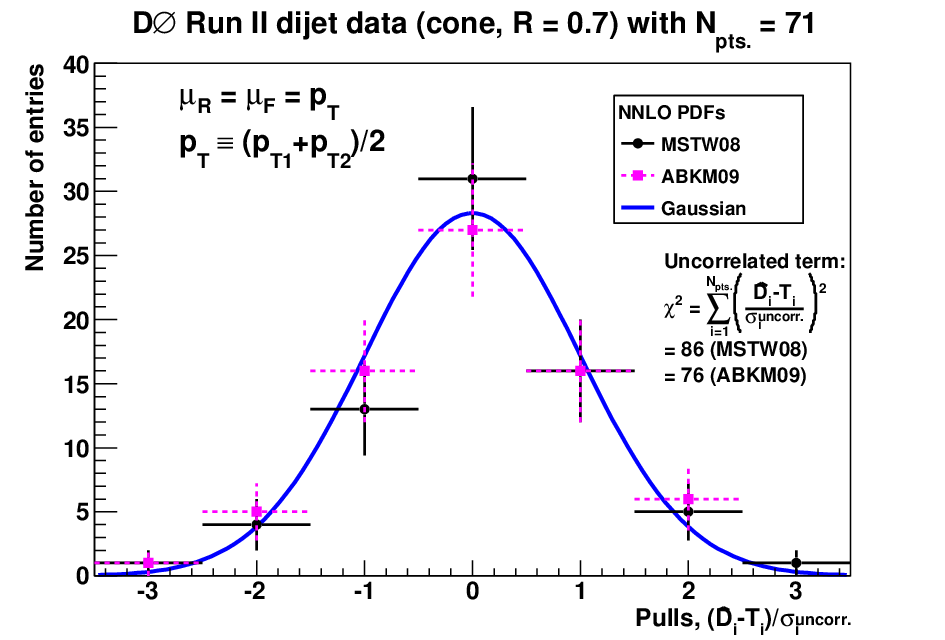
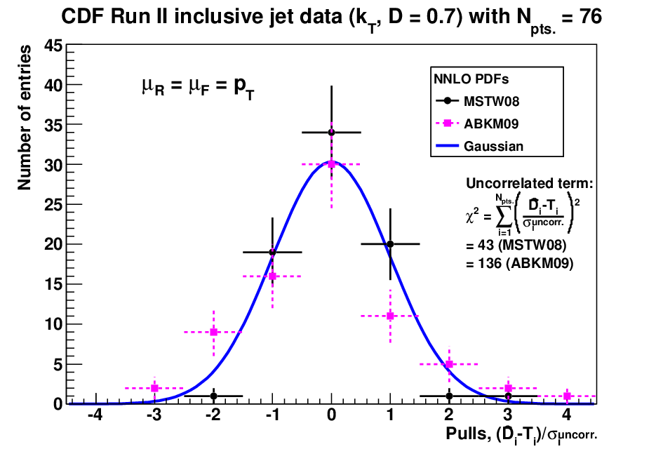
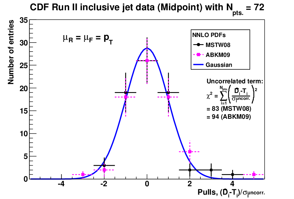
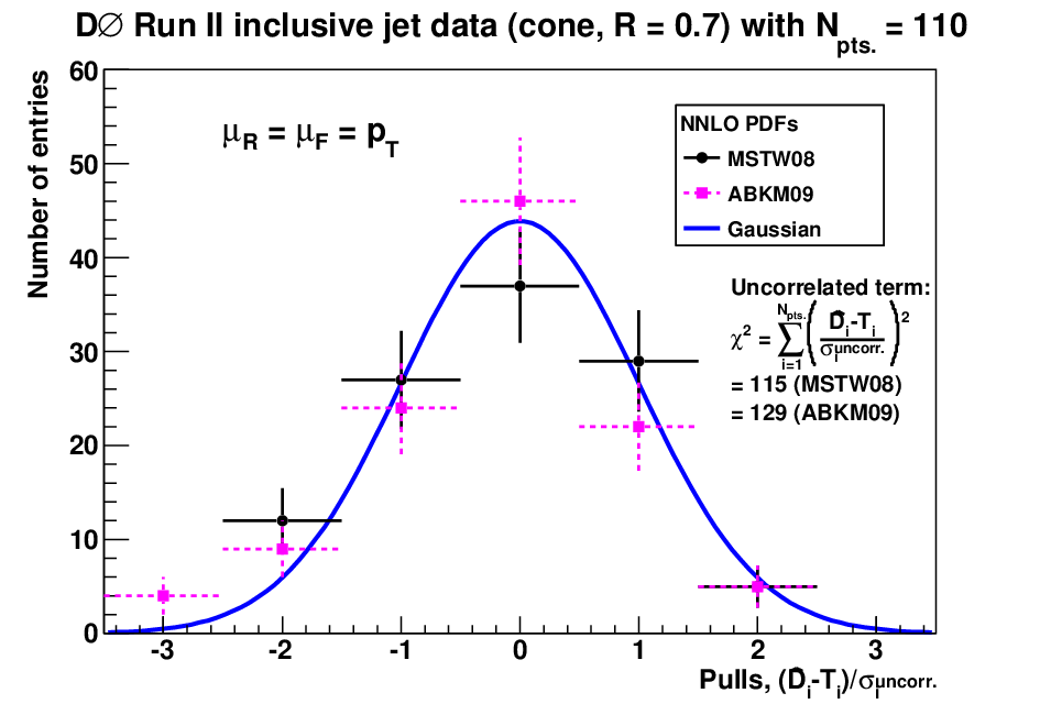
In figure 16 we show the distributions of pulls, , for all four Tevatron Run II data sets on jet production, with theory predictions calculated using either MSTW08 or ABKM09 NNLO PDFs and a scale choice . We show the expected behaviour of a Gaussian distribution with unit width, and the first term in eq. (2) given simply by the sum of pulls over all data points. The histogram error bars are simply given by the square root of the number of entries. We see that the distribution of pulls is fairly close to the expected Gaussian behaviour for all four data sets, although the tails for the inclusive jet data with ABKM09 are somewhat broader than expected, leading to larger contributions than for MSTW08, particularly for the CDF data using the jet algorithm [33] shown in figure 16(a). However, it is clear that this source does not account for the complete differences in seen previously.
(a)

(b)

(c)

(d)

In figure 17 we show the similar distributions of the systematic shifts, , again for all four Tevatron Run II data sets on jet production. We show the expected behaviour of a Gaussian distribution with unit width and the penalty term simply given by the sum of the values. For the inclusive jet data, the systematic shifts for MSTW08 show the expected Gaussian behaviour, with small penalty terms . On the other hand, the systematic shifts for ABKM09 deviate substantially from Gaussian behaviour, with much larger penalty terms, in particular for the CDF inclusive jet data using the algorithm shown in figure 17(a). The systematic shifts for the dijet data shown in figure 17(d) have a much narrower distribution than the expected Gaussian behaviour for both MSTW08 and ABKM09, suggesting that the systematic errors are overestimated, are non-Gaussian, or are not independent (or a combination of these three explanations). Note that the number of systematic sources () for the dijet data is much greater than for any of the inclusive jet data sets. Indeed, this allows the value of for the description of data by an identically zero theory prediction to be lower than for some of the PDF sets; see table 4.
The presentation of the results in figures 16 and 17 enables a separation between contributions to the definition, eq. (2), from uncorrelated and correlated errors, respectively. This allows a more informed assessment of the fit quality compared to the more traditional definition of eq. (7) in terms of the experimental covariance matrix, used by the ABKM and NNPDF fitting groups; see also appendix B.3 of ref. [42] and section 4 of ref. [18].
3.6 Other jet cross sections from collider experiments
The DØ Collaboration has recently made a measurement [65] of the three-jet differential cross section as a function of the invariant mass of the three jets with the largest transverse momentum in an event. An exercise has been carried out similar to the one presented here, where the has been evaluated for different PDF (and ) choices and scale choices , where the mean jet . The trend is that MSTW08 and NNPDF2.1 are favoured, as for the inclusive jet study presented here, while ABKM09 is worse, and CT10 and HERAPDF1.0 are still poorer. We have followed a similar approach to that of ref. [65] by evaluating the only for the central PDF fit, without accounting for PDF uncertainties. Since the Tevatron jet data provide by far the most direct constraint on the high- gluon distribution, the agreement of the central PDF fit is more important and relevant than obtaining agreement only within possibly large PDF uncertainties. However, the potential choice of scales for the three-jet cross section is even broader than for the dijet cross section.
The LHC data on jet production [66, 67, 68, 69] are becoming more precise and show some sensitivity to the PDF choice. However, these data are still being understood and are not presented with separated correlated systematic uncertainties which would allow a quantitative comparison. Moreover, the general sensitivity is to lower , and so less relevant for Higgs production at the Tevatron. Isolated photon production at the LHC may also provide a direct constraint on the gluon distribution [70]. The HERA jet data are less sensitive to the gluon distribution at high values, being more of a constraint for –, and there is no NNLO calculation, or any approximation such as the 2-loop threshold corrections available for the Tevatron inclusive jet data.
3.7 Summary
Comparison with Tevatron jet data is subtle because of the large correlated systematic uncertainties. The systematic shifts, eq. (3), can compensate for inadequacies in the theory calculation. The traditional definition in terms of the experimental covariance matrix, eq. (7), can hide such systematic shifts. In particular, we find that the Tevatron jet data need to be normalised downwards by typically between 3- and 5- (see appendix A) to achieve the best agreement with some PDF sets, particularly the ABKM09 predictions. Even if the luminosity shift is artificially constrained, the other systematic shifts move by large amounts for the inclusive jet data, incompatible with the Gaussian expectation. No such problems are observed for the MSTW08 predictions. It can also be seen from the plots in ref. [12] that the unshifted Tevatron jet data lie significantly above the theory predictions even after including these data in variants of the ABKM09 fit. Constraining the Tevatron luminosity shifts, for example, so that the predicted and cross sections agreed with Tevatron data, would increase the constraining power of the Tevatron jet data and thereby very likely give a larger and high- gluon distribution than the current studies of Alekhin, Blümlein and Moch (ABM) [12]. Even with the existing treatment, the NNLO Tevatron cross section for GeV goes up by when including the {CDF [33], CDF Midpoint [34], DØ inclusive [35], DØ dijet [36]} data set in variants of the ABKM09 fit [12]. The dijet data has a potentially wider range of allowed scale choices than the inclusive jet data. We conclude that the data on inclusive jet production therefore provide the cleanest probe of different PDF sets.
4 Value of strong coupling from DIS
There is a common lore (see, for example, ref. [71]) that DIS-only fits prefer low values, but ref. [32] showed that not all DIS data sets prefer low values. In particular, this was found to be true only for BCDMS data, and for E665 and SLAC data, while NMC, SLAC and HERA data preferred high values within the context of the global fit [32]. (See also the recent NNPDF study at NLO using an “unbiased” PDF parameterisation [72].)
It is well known that is highly anticorrelated with the low- gluon distribution through scaling violations of HERA data: . Then is correlated with the high- gluon distribution through the momentum sum rule; see, for example, figure 14(b) of ref. [32]. Restrictive gluon parameterisations, without the negative small- term allowed by MSTW [13], can therefore bias the extracted value. For example, the default MSTW08 NNLO fit obtained , while imposing the restriction of a positive input gluon at GeV2 gave a best-fit , but with a worse by 63 units for the global fit to 2615 data points [32].55 5 The values for the increase of 80 at NLO and 63 at NNLO were erroneously interchanged in ref. [32].
What is from only DIS data in the MSTW08 NNLO fit?66 6 Studies prompted by question from G. Altarelli, December 2010. Recall that the global fit gave [32]. To expand on the studies made in ref. [32], we performed a new NNLO DIS-only fit, which gave a best-fit , but with an input gluon distribution which went negative for due to lack of any data constraint. This implies a negative charm structure function, , and a terrible description ( including correlated systematic errors) of Tevatron jet data using the obtained PDFs. A DIS-only fit fixing the high- gluon parameters to prevent such bad behaviour gave , i.e. very similar to the global fit. However, a NNLO fit which imposed the condition of the positive low- gluon, which stopped the gluon from going negative at high values, and which also omitted the Tevatron jet data, gave , rather closer to the ABKM09 value. The very low value of found in the DIS-only fit is due to the dominance of BCDMS data. We can show this explicitly by removing the BCDMS data from the DIS-only fit, then the best-fit moves from to . Repeating the global fit with BCDMS data removed gives , i.e. a change by less than the quoted experimental uncertainty of . The conclusion is that the Tevatron jet data are vital to pin down the high- gluon, giving a smaller low- gluon and therefore a larger in the global fit compared to a DIS-only fit, at the expense of some deterioration in the fit quality of the BCDMS data.77 7 The low data points from BCDMS are strongly affected by the energy scale uncertainty of the scattered muon. It has been advocated to impose a cut of on the BCDMS data, which caused to increase by about 0.004 in a fit to only BCDMS data and by about 0.002 in a combined fit to H1 and BCDMS data [73]. The benefits of including the Tevatron jet data to obtain sensible results in a simultaneous fit of PDFs and therefore greatly outweighs any disadvantage such as lack of complete NNLO corrections.
The only input DIS value to the current world average [31] is the BBG06 value [74], which is from a non-singlet analysis and therefore in principle free of assumptions made about the gluon distribution. A value of
| (11) |
was obtained at {NLO, NNLO, N3LO}, by fitting proton and deuteron structure functions, and , for (assuming only valence quarks, neglecting the singlet contribution), and the less precise for . However, using the MSTW08 NNLO central fit, contributions other than valence quarks are found to make up about () of at (). As an exercise we performed the MSTW08 NNLO DIS-only fit just to and for (comprising 282 data points, 160 of these from BCDMS), which gave () without (with) the singlet contribution included. This is even lower than the BBG06 value presumably due to lack of the cut on BCDMS data applied in the BBG06 analysis. The low value of found by BBG06 [74] is therefore due to both dominance of BCDMS data and by what we conclude is the unjustified neglect of the singlet contribution to and for . Given that it was argued above that the Tevatron jet data are needed to pin down the high- gluon, we conclude that an extraction of only from inclusive DIS data is not meaningful, and the closest possible to a reliable extraction is the MSTW08 NNLO combined analysis of DIS, Drell–Yan and jet data [13, 32]:
| (12) |
This value is the only NNLO determination, from a simultaneous fit with PDFs, which is in agreement with the current world average [31]; see figure 5(b).
5 Treatment of NMC data and stability to low data
A recent claim has been made [11] that the bulk of the MSTW08/ABKM09 difference in both the extracted value and the predictions is explained by the treatment of NMC data [14]. The differential cross section for DIS of charged leptons off nucleons, , neglecting the nucleon and lepton masses, and assuming single-photon exchange, is
| (13) |
where is the ratio of the cross sections for longitudinally and transversely polarised photons, is the photon virtuality, is the Bjorken variable and is the inelasticity (with the centre-of-mass energy). The ABKM09 [15] analysis fitted the NMC differential cross sections directly, calculating to and including empirical higher-twist corrections. The MSTW08 [13] analysis instead fitted the NMC values corrected for , where [14]
| (14) |
Here, was a (-independent) value extracted from NMC data, while was a -dependent empirical parameterisation of SLAC data dating from 1990 [75]. By replacing the NMC differential cross-section data by NMC data, ABM [11] find that their best-fit moves from 0.1135 to 0.1170 and their cross sections at the Tevatron and LHC move closer to the MSTW08 values. ABM [11] therefore conclude that the use of NMC data in the MSTW08 fit rather than the differential cross section is the main reason for the higher and Higgs cross sections obtained with MSTW08.
(a)

(b)

We agree that it is more consistent to fit directly to the NMC differential cross-section data, so here we respond to this rather dramatic assertion made by ABM [11], which would obviously be very worrying if correct. However, rather than repeat the MSTW08 analysis by fitting the NMC differential cross sections, we note that the original NMC paper [14] made an alternative extraction of values using the SLAC parameterisation [75]. In figure 18(a) we compare with in the most affected bin of , i.e. a low value where there are a reasonable number (7) of NMC data points surviving the cut on GeV2 and where the difference between and is at its largest. Recall that a low value means a high value and from eq. (13) the correction term from is only important at large . In figure 18(a) we also show the MSTW08 NNLO prediction, including PDF uncertainties at 68% C.L., with calculated to and without any higher-twist corrections. We see that it gives a good description of the SLAC parameterisation, with any differences being very much smaller than those between and . We note that NMC/BCDMS/SLAC data are included in the MSTW08 fit and are well-described at NNLO but less well at NLO (see figure 5 of ref. [32]), so the coefficient functions are needed for a good description and the larger MSTW08 perhaps explains why there is less room for higher-twist corrections, contrary to the findings of the ABM analysis. Nevertheless, figure 18(a) demonstrates that fitting the alternative NMC data extracted using the SLAC parameterisation will give very similar results to fitting the NMC differential cross sections. In fact, given that in figure 18(a) generally has a slightly steeper dependence than the MSTW08 parameterisation, using this will slightly overestimate the true impact of fitting the NMC differential cross sections. In figure 18(b) we compare the two different NMC extractions, again for the most affected bin of , and we see that there is little difference, certainly nothing that seems likely to change by in a fit where it is constrained with an uncertainty of about by over 2000 other data points.
| NNLO PDF | at Tevatron | at 7 TeV LHC | |
|---|---|---|---|
| MSTW08 | 0.1171 | 0.342 pb | 7.91 pb |
| Use for NMC | |||
| Cut NMC () | |||
| Cut all NMC data | |||
| Cut GeV2, GeV2 | |||
| Cut GeV2, GeV2 | |||
| Fix | |||
| Input , no jets | |||
| ABKM09 | 0.1135 |

In table 5 we show the effect of repeating the MSTW08 NNLO fit with the NMC data extracted using on and the Higgs cross sections (for GeV) at the Tevatron and LHC, and in figure 19 we show the change in the gluon distribution at the corresponding scale. We make other fits either cutting the NMC data for , above which the correction in eq. (13) is very small indeed, or completely removing all NMC data. In all cases there is very little change in , the gluon distribution, and the Higgs cross section. We conclude that the treatment of NMC data cannot explain the difference between the MSTW08 and ABKM09 results. Similar stability has been found by the NNPDF group [76], but in a less relevant study at NLO with fixed .
The cuts on DIS data are not explicitly given in the ABKM09 paper [15], but the previous AMP06 paper [77] mentions that DIS data are removed with GeV2 and , compared to the MSTW08 fit which removes DIS data with GeV2 and . The much weaker cut on the hadronic invariant mass (squared), , clearly explains why higher-twist corrections are more important in the ABKM09 analysis. To investigate the possible effect of neglected higher-twist corrections on the MSTW08 NNLO fit we raised the cuts to remove DIS data with GeV2 and either GeV2 or GeV2. The results are shown in table 5 and figure 19. The changes in , the gluon distribution and the Higgs cross sections are generally small and within uncertainties, although with the strongest cut there is no data constraint below and little just above, so the PDFs differ but have large uncertainties at low values.88 8 We also investigated the effect of increasing the cuts on and in variants of the MSTW NLO fit. The changes were slightly bigger, with changing from 0.1202 to 0.1192 and 0.1175 with cuts of 5 and 10 GeV2, respectively. Similarly, the changes in PDFs and cross-section predictions are generally slightly greater at NLO than at NNLO, i.e. as expected there is some improved stability at higher orders.
In table 5 and figure 19 we show the results of the MSTW08 NNLO fit with a fixed [32] (slightly below the ABKM09 value), and even in this case the gluon distribution and Higgs cross sections move only part of the way towards the ABKM09 result, as already seen in figure 7. The MSTW08 input gluon parameterisation is [13]
| (15) |
compared to the much more restrictive functional forms of the other NNLO fits, namely:
| ABKM09 [15]: | (16) | |||
| JR09 [21]: | (17) | |||
| HERAPDF1.0 [23]: | (18) |
The normalisation is determined from the momentum sum rule constraint, leaving 7 free parameters for MSTW08 compared to only 3 for ABKM09 and only 2 for JR09 and HERAPDF1.0 (although the value of is optimised in the case of JR09). In the lack of any direct data constraint on the high- gluon distribution, the other fits are therefore constrained by the form of the input parameterisation, avoiding the pathological behaviour of the negative high- gluon distribution seen for the MSTW08 NNLO DIS-only fit described in section 4. As already mentioned in that section, in an attempt to mimic the ABKM09 fit we performed a variant of the MSTW08 NNLO fit without jet data and with the second term of eq. (15) set to zero. The and parameters were fixed in the fit iteration before the high- gluon distribution went negative. The results of this fit are shown in table 5 and figure 19 and it goes some way towards reproducing the high- gluon of the ABKM09 fit and the corresponding Tevatron prediction, certainly closer than we come with other modifications. Finally, we then investigated the effect of using NMC data corrected using rather than in this fit. Similar to our default fit all changes were at the percent level, or less, so we do not explicitly show them, although the gluon does move marginally closer again to that of ABKM09.
Other differences between the two analyses are that ABKM09 used the NMC data for separate muon beam energies, whereas MSTW08 used the NMC data averaged over beam energies, which reduces the maximum effect of the change in for a particular data point, i.e. at a given and , a data point at high , and so very sensitive to at a low beam energy, is at lower for a higher beam energy. In the case of the averaged NMC data, correlated systematic uncertainties are unavailable, so the MSTW08 fit simply added errors (other than normalisation) in quadrature similar to the simple form of eq. (8). As with the Tevatron jet data, deficiencies in the theory calculation may be hidden, without much trace, by large systematic shifts implicit in the definition, eq. (7), similar to that used in the ABKM09 analysis. We conclude that the greater sensitivity to the treatment of NMC data found by ABM [11] is due to a variety of reasons, but perhaps most significantly, the inclusion of higher-twist corrections due to the weaker cuts on DIS data, and, as we have repeatedly emphasised, the lack of additional constraints provided by the Tevatron jet data to pin down the high- gluon distribution.
6 Conclusions
The anomalously large higher-order QCD corrections to Higgs production at the Tevatron and LHC, via the dominant production channel of gluon–gluon fusion through a top-quark loop, mandate the use of (at least) NNLO calculations, together with corresponding NNLO PDFs and values. The Tevatron Higgs cross section, in particular, requires knowledge of the gluon distribution at large where constraints from DIS or Drell–Yan data are weak and the only direct constraint comes from Tevatron inclusive jet production. The MSTW08 fit [13] is currently the only public NNLO PDF set including the Tevatron jet data, and is used in the analyses of the Tevatron [4, 5] and LHC [3] experiments, while other NNLO PDF fitting groups (ABKM09 [15], JR09 [21, 22], HERAPDF1.0 [23]) choose to omit it, finding quite different results for the predicted Higgs cross sections. This common choice to use only the MSTW08 set, and not the other publicly available NNLO PDF sets, has faced a barrage of recent criticism [7, 8, 9, 10, 11, 12], which we have responded to in detail in this paper. We summarise our main findings below:
- •
- •
The claim [9] that the HERAPDF1.0 NNLO set with lowers the Higgs cross section compared to MSTW08 by for GeV at the Tevatron is due to a mistake in the calculation, and therefore the conclusions in the published version of ref. [9] are flawed. On the other hand, the observed 25% reduction with the central value of ABKM09 is still a serious problem and we give evidence in this paper that the ABKM09 set is not consistent enough with existing Tevatron data to be used for the calculation of Higgs cross sections.
- •
Comparison with Tevatron jet data is subtle because of the large correlated systematic uncertainties and the need to make choices in luminosity which are consistent with the predictions for and cross sections. The traditional definition in terms of the experimental covariance matrix, eq. (7), can hide large systematic shifts, which can compensate for inadequacies in the theory calculation. In particular, we find that the Tevatron jet data need to be normalised downwards by typically between 3- and 5- to achieve the best agreement with the ABKM09 (and some HERAPDF) predictions; see appendix A. Even if the luminosity shift is artificially constrained, the other systematic shifts move by large amounts for the inclusive jet data, incompatible with the Gaussian expectation. No such problems are observed for the MSTW08 predictions and good agreement is found with all Run II inclusive jet data, and also with the dijet data if taking a larger scale choice than for the inclusive jet data.
- •
We have demonstrated that the MSTW08 fit is stable to the treatment of NMC data, unlike the ABKM09 fit [11], most likely because of the averaging over muon beam energies, because the Tevatron jet data pin down the high- gluon distribution, and also due to the stronger cuts reducing the need for large higher-twist corrections. Moreover, the MSTW08 NNLO determination of the strong coupling is compatible with the world average value, unlike other NNLO determinations shown in figure 5(b).
We conclude that the current Tevatron Higgs exclusion bounds [4, 5] are robust, at least with respect to the treatment of PDFs and in the calculation of the Higgs cross section. Similar remarks hold for the Higgs cross sections at the LHC recently calculated in ref. [3].
Appendix A Appendix: tables with unrestricted luminosity shifts
For completeness, in tables 6, 7, 8 and 9 we show values without the restriction in the luminosity shifts of imposed in the main tables given in section 3. Recall from eq. (3) that a positive value of means a downwards shift in the luminosity, so we choose to give in brackets the values of “”, i.e. negative numbers correspond to downwards shifts in the luminosity. In the table captions we give the values with an identically zero theory prediction () just to illustrate an extreme case of how large downwards luminosity shifts can partially accommodate an inadequate theory prediction.
| NLO PDF (with NLO ) | |||
|---|---|---|---|
| MRST04 | 1.05 (1.25) | 0.94 (0.02) | 0.77 (1.83) |
| MSTW08 | 0.75 (0.32) | 0.68 (0.88) | 0.63 (2.69) |
| CTEQ6.6 | 1.03 (2.47) | 1.04 (3.49) | 0.99 (4.75) |
| CT10 | 0.99 (1.64) | 0.92 (2.69) | 0.86 (4.10) |
| NNPDF2.1 | 0.74 (0.33) | 0.79 (1.60) | 0.80 (3.12) |
| HERAPDF1.0 | 1.52 (4.07) | 1.57 (5.21) | 1.43 (6.22) |
| HERAPDF1.5 | 1.48 (3.85) | 1.52 (5.00) | 1.39 (6.03) |
| ABKM09 | 1.03 (3.49) | 1.01 (4.53) | 1.05 (5.80) |
| GJR08 | 1.14 (2.47) | 0.93 (1.25) | 0.79 (0.50) |
| NNLO PDF (with NLO+2-loop ) | |||
| MRST06 | 2.80 (2.23) | 1.20 (1.34) | 1.03 (0.53) |
| MSTW08 | 1.39 (0.35) | 0.69 (0.45) | 0.97 (1.30) |
| HERAPDF1.0, | 2.37 (2.65) | 1.48 (3.64) | 1.29 (4.12) |
| HERAPDF1.0, | 2.24 (0.48) | 1.13 (1.60) | 1.09 (2.23) |
| ABKM09 | 1.53 (4.27) | 1.23 (5.05) | 1.44 (5.65) |
| JR09 | 0.75 (0.13) | 1.26 (0.61) | 2.20 (1.22) |
| NLO PDF (with NLO ) | |||
|---|---|---|---|
| MRST04 | 2.14 (1.40) | 2.01 (0.02) | 1.57 (1.38) |
| MSTW08 | 1.52 (1.05) | 1.40 (0.31) | 1.15 (1.74) |
| CTEQ6.6 | 1.93 (1.46) | 1.90 (2.50) | 1.58 (3.41) |
| CT10 | 1.75 (0.63) | 1.67 (1.76) | 1.39 (2.82) |
| NNPDF2.1 | 1.69 (0.30) | 1.56 (1.01) | 1.40 (2.20) |
| HERAPDF1.0 | 2.49 (2.84) | 2.45 (3.86) | 2.11 (4.54) |
| HERAPDF1.5 | 2.39 (2.68) | 2.36 (3.72) | 2.05 (4.42) |
| ABKM09 | 1.52 (2.05) | 1.53 (3.10) | 1.38 (4.04) |
| GJR08 | 2.02 (2.60) | 1.75 (1.18) | 1.52 (0.26) |
| NNLO PDF (with NLO+2-loop ) | |||
| MRST06 | 2.72 (2.83) | 2.07 (1.14) | 2.11 (0.12) |
| MSTW08 | 1.66 (1.54) | 1.39 (0.06) | 1.62 (1.00) |
| HERAPDF1.0, | 2.20 (1.15) | 1.99 (2.45) | 2.04 (3.06) |
| HERAPDF1.0, | 2.08 (0.63) | 1.76 (0.97) | 1.96 (1.78) |
| ABKM09 | 1.63 (2.42) | 1.73 (3.50) | 1.93 (4.15) |
| JR09 | 1.57 (0.87) | 2.05 (0.55) | 2.81 (1.44) |
| NLO PDF (with NLO ) | |||
|---|---|---|---|
| MRST04 | 1.76 (1.58) | 1.34 (0.09) | 0.98 (1.77) |
| MSTW08 | 1.40 (1.05) | 1.08 (0.55) | 0.85 (2.25) |
| CTEQ6.6 | 1.52 (1.61) | 1.25 (2.88) | 1.01 (4.02) |
| CT10 | 1.39 (0.66) | 1.11 (2.02) | 0.90 (3.35) |
| NNPDF2.1 | 1.41 (0.37) | 1.23 (1.22) | 0.95 (2.67) |
| HERAPDF1.0 | 1.55 (2.16) | 1.38 (3.51) | 1.07 (4.52) |
| HERAPDF1.5 | 1.63 (1.98) | 1.45 (3.35) | 1.12 (4.40) |
| ABKM09 | 1.25 (1.90) | 1.04 (3.20) | 0.89 (4.44) |
| GJR08 | 1.72 (2.14) | 1.34 (0.53) | 0.98 (1.05) |
| NNLO PDF (with NLO+2-loop ) | |||
| MRST06 | 2.92 (2.66) | 1.70 (1.31) | 1.25 (0.44) |
| MSTW08 | 1.87 (1.34) | 1.23 (0.09) | 1.08 (0.87) |
| HERAPDF1.0, | 2.11 (0.82) | 1.52 (2.03) | 1.14 (2.61) |
| HERAPDF1.0, | 2.28 (0.94) | 1.50 (0.49) | 1.11 (1.23) |
| ABKM09 | 1.48 (2.33) | 1.13 (3.35) | 1.02 (4.03) |
| JR09 | 1.84 (0.63) | 1.61 (0.60) | 1.50 (1.35) |
| NLO PDF (with NLO ) | |||
|---|---|---|---|
| MRST04 | 5.79 (3.58) | 4.52 (1.73) | 2.75 (0.01) |
| MSTW08 | 3.03 (2.82) | 2.25 (1.11) | 1.56 (0.61) |
| CTEQ6.6 | 5.41 (0.62) | 4.85 (0.92) | 3.31 (2.14) |
| CT10 | 4.74 (1.33) | 4.06 (0.24) | 2.68 (1.62) |
| NNPDF2.1 | 2.59 (2.41) | 1.93 (0.79) | 1.47 (0.75) |
| HERAPDF1.0 | 2.05 (0.66) | 2.17 (2.06) | 1.94 (3.11) |
| HERAPDF1.5 | 1.90 (0.46) | 1.97 (1.85) | 1.73 (2.93) |
| ABKM09 | 1.49 (0.17) | 1.39 (1.58) | 1.21 (2.83) |
| GJR08 | 10.2 (4.48) | 7.79 (2.78) | 5.30 (1.07) |
| NNLO PDF (with NLO ) | |||
| MRST06 | 7.87 (3.19) | 6.55 (1.42) | 4.07 (0.13) |
| MSTW08 | 2.34 (1.96) | 1.80 (0.42) | 1.31 (1.12) |
| HERAPDF1.0, | 2.61 (0.09) | 2.55 (1.44) | 2.31 (2.51) |
| HERAPDF1.0, | 2.71 (1.53) | 2.31 (0.04) | 1.95 (1.37) |
| ABKM09 | 1.35 (1.36) | 1.40 (2.56) | 1.31 (3.60) |
| JR09 | 3.27 (1.75) | 2.55 (0.33) | 1.88 (1.08) |
Acknowledgements.
We thank A. D. Martin and W. J. Stirling for numerous discussions, and S. Alekhin, G. Hesketh, D. Waters and M. Wobisch for useful information. The work of R.S.T. is supported partly by the London Centre for Terauniverse Studies (LCTS), using funding from the European Research Council via the Advanced Investigator Grant 267352.References
- (1) C. Anastasiou, R. Boughezal, and F. Petriello, Mixed QCD-electroweak corrections to Higgs boson production in gluon fusion, JHEP 04 (2009) 003, [arXiv:0811.3458].
- (2) D. de Florian and M. Grazzini, Higgs production through gluon fusion: updated cross sections at the Tevatron and the LHC, Phys. Lett. B674 (2009) 291–294, [arXiv:0901.2427].
- (3) LHC Higgs Cross Section Working Group, S. Dittmaier, C. Mariotti, G. Passarino, and R. Tanaka (Eds.), Handbook of LHC Higgs Cross Sections: 1. Inclusive Observables, CERN-2011-002 (CERN, Geneva, 2011) [arXiv:1101.0593].
- (4) CDF and DØ Collaboration, TEVNPHWG, Combined CDF and DØ Upper Limits on Standard Model Higgs Boson Production with up to 6.7 fb-1 of Data, arXiv:1007.4587.
- (5) CDF and DØ Collaboration, TEVNPHWG, Combined CDF and DØ Upper Limits on Standard Model Higgs Boson Production with up to 8.2 fb-1 of Data, arXiv:1103.3233.
- (6) G. Watt, Parton distribution function dependence of benchmark Standard Model total cross sections at the 7 TeV LHC, arXiv:1106.5788.
- (7) J. Baglio and A. Djouadi, Predictions for Higgs production at the Tevatron and the associated uncertainties, JHEP 10 (2010) 064, [arXiv:1003.4266].
- (8) J. Baglio and A. Djouadi, Higgs production at the lHC, JHEP 03 (2011) 055, [arXiv:1012.0530].
- (9) J. Baglio, A. Djouadi, S. Ferrag, and R. M. Godbole, The Tevatron Higgs exclusion limits and theoretical uncertainties: a critical appraisal, Phys. Lett. B699 (2011) 368–371, [arXiv:1101.1832].
- (10) S. Alekhin, J. Blümlein, P. Jimenez-Delgado, S.-O. Moch, and E. Reya, NNLO Benchmarks for Gauge and Higgs Boson Production at TeV Hadron Colliders, Phys. Lett. B697 (2011) 127–135, [arXiv:1011.6259].
- (11) S. Alekhin, J. Blümlein, and S.-O. Moch, Higher order constraints on the Higgs production rate from fixed-target DIS data, arXiv:1101.5261.
- (12) S. Alekhin, J. Blümlein, and S.-O. Moch, Parton distributions and Tevatron jet data, arXiv:1105.5349.
- (13) A. D. Martin, W. J. Stirling, R. S. Thorne, and G. Watt, Parton distributions for the LHC, Eur.Phys.J. C63 (2009) 189–285, [arXiv:0901.0002].
- (14) New Muon Collaboration, M. Arneodo et. al., Measurement of the proton and deuteron structure functions, and , and of the ratio , Nucl. Phys. B483 (1997) 3–43, [hep-ph/9610231].
- (15) S. Alekhin, J. Blümlein, S. Klein, and S.-O. Moch, The 3, 4, and 5-flavor NNLO Parton from Deep-Inelastic-Scattering Data and at Hadron Colliders, Phys.Rev. D81 (2010) 014032, [arXiv:0908.2766].
- (16) A. Djouadi, M. Spira, and P. M. Zerwas, Production of Higgs bosons in proton colliders: QCD corrections, Phys.Lett. B264 (1991) 440–446.
- (17) P. M. Nadolsky, H.-L. Lai, Q.-H. Cao, J. Huston, J. Pumplin, D. Stump, W.-K. Tung, and C.-P. Yuan, Implications of CTEQ global analysis for collider observables, Phys.Rev. D78 (2008) 013004, [arXiv:0802.0007].
- (18) H.-L. Lai, M. Guzzi, J. Huston, Z. Li, P. M. Nadolsky, J. Pumplin, and C.-P. Yuan, New parton distributions for collider physics, Phys.Rev. D82 (2010) 074024, [arXiv:1007.2241].
- (19) NNPDF Collaboration, R. D. Ball et. al., Impact of Heavy Quark Masses on Parton Distributions and LHC Phenomenology, Nucl. Phys. B849 (2011) 296–363, [arXiv:1101.1300].
- (20) R. V. Harlander and W. B. Kilgore, Next-to-next-to-leading order Higgs production at hadron colliders, Phys. Rev. Lett. 88 (2002) 201801, [hep-ph/0201206]. ggh@nnlo code from http://particle.uni-wuppertal.de/harlander/software/ggh@nnlo/.
- (21) P. Jimenez-Delgado and E. Reya, Dynamical NNLO parton distributions, Phys.Rev. D79 (2009) 074023, [arXiv:0810.4274].
- (22) P. Jimenez-Delgado and E. Reya, Variable Flavor Number Parton Distributions and Weak Gauge and Higgs Boson Production at Hadron Colliders at NNLO of QCD, Phys.Rev. D80 (2009) 114011, [arXiv:0909.1711].
- (23) H1 and ZEUS Collaboration, F. D. Aaron et. al., Combined Measurement and QCD Analysis of the Inclusive Scattering Cross Sections at HERA, JHEP 1001 (2010) 109, [arXiv:0911.0884].
- (24) R. S. Thorne, A. D. Martin, W. J. Stirling, and G. Watt, The effects of combined HERA and recent Tevatron charge asymmetry data on the MSTW PDFs, PoS DIS2010 (2010) 052, [arXiv:1006.2753].
- (25) S. Forte, Parton distributions at the dawn of the LHC, Acta Phys. Polon. B41 (2010) 2859–2920, [arXiv:1011.5247].
- (26) S. Alekhin et. al., The PDF4LHC Working Group Interim Report, arXiv:1101.0536.
- (27) A. De Roeck and R. S. Thorne, Structure Functions, Progress in Particle and Nuclear Physics (2011) [arXiv:1103.0555].
- (28) M. Botje et. al., The PDF4LHC Working Group Interim Recommendations, arXiv:1101.0538.
- (29) ATLAS Collaboration, A combined measurement of the top quark pair production cross-section using dilepton and single-lepton final states, 22nd March 2011. ATLAS-CONF-2011-040.
- (30) CMS Collaboration, Combination of top pair production cross sections in collisions at TeV and comparisons with theory, 16th March 2011. CMS PAS TOP-11-001.
- (31) S. Bethke, The 2009 World Average of , Eur.Phys.J. C64 (2009) 689–703, [arXiv:0908.1135].
- (32) A. D. Martin, W. J. Stirling, R. S. Thorne, and G. Watt, Uncertainties on in global PDF analyses and implications for predicted hadronic cross sections, Eur.Phys.J. C64 (2009) 653–680, [arXiv:0905.3531].
- (33) CDF Collaboration, A. Abulencia et. al., Measurement of the Inclusive Jet Cross Section using the algorithm in Collisions at TeV with the CDF II Detector, Phys. Rev. D75 (2007) 092006, [hep-ex/0701051].
- (34) CDF Collaboration, T. Aaltonen et. al., Measurement of the Inclusive Jet Cross Section at the Fermilab Tevatron Collider Using a Cone-Based Jet Algorithm, Phys. Rev. D78 (2008) 052006, [arXiv:0807.2204].
- (35) DØ Collaboration, V. M. Abazov et. al., Measurement of the inclusive jet cross-section in collisions at TeV, Phys. Rev. Lett. 101 (2008) 062001, [arXiv:0802.2400].
- (36) DØ Collaboration, V. M. Abazov et. al., Measurement of the dijet invariant mass cross section in proton anti-proton collisions at TeV, Phys. Lett. B693 (2010) 531–538, [arXiv:1002.4594].
- (37) N. Kidonakis and J. F. Owens, Effects of higher-order threshold corrections in high- jet production, Phys. Rev. D63 (2001) 054019, [hep-ph/0007268].
- (38) T. Kluge, K. Rabbertz, and M. Wobisch, Fast pQCD calculations for PDF fits, hep-ph/0609285. fastnlo code from http://projects.hepforge.org/fastnlo/.
- (39) Z. Nagy, Three-jet cross sections in hadron hadron collisions at next-to-leading order, Phys. Rev. Lett. 88 (2002) 122003, [hep-ph/0110315].
- (40) Z. Nagy, Next-to-leading order calculation of three jet observables in hadron hadron collision, Phys. Rev. D68 (2003) 094002, [hep-ph/0307268].
- (41) D. Stump, J. Pumplin, R. Brock, D. Casey, J. Huston, et. al., Uncertainties of predictions from parton distribution functions. 1. The Lagrange multiplier method, Phys.Rev. D65 (2001) 014012, [hep-ph/0101051].
- (42) J. Pumplin et. al., New generation of parton distributions with uncertainties from global QCD analysis, JHEP 07 (2002) 012, [hep-ph/0201195].
- (43) A. D. Martin, W. J. Stirling, R. S. Thorne, and G. Watt, Heavy-quark mass dependence in global PDF analyses and 3- and 4-flavour parton distributions, Eur. Phys. J. C70 (2010) 51–72, [arXiv:1007.2624].
- (44) V. Papadimitriou, Luminosity measurements at hadron colliders, Nucl. Instrum. Meth. A598 (2009) 14–18.
- (45) H. Burkhardt, M. Ferro-Luzzi, A. Macpherson, and M. Mangano (Eds.), LHC Lumi Days: LHC Workshop on LHC Luminosity Calibration, 2011. CERN-Proceedings-2011-001.
- (46) CDF Collaboration, A. Abulencia et. al., Measurements of Inclusive and Cross Sections in Collisions at TeV, J. Phys. G34 (2007) 2457–2544, [hep-ex/0508029].
- (47) CDF Collaboration, T. A. Aaltonen et. al., Measurement of of Drell–Yan pairs in the Mass Region from Collisions at TeV, Phys. Lett. B692 (2010) 232–239, [arXiv:0908.3914].
- (48) DØ Collaboration, V. M. Abazov et. al., Measurement of differential +jet+X cross sections in collisions at TeV, Phys. Lett. B669 (2008) 278–286, [arXiv:0808.1296].
- (49)
C. Anastasiou, L. J. Dixon, K. Melnikov, and F. Petriello, High precision
QCD at hadron colliders: Electroweak gauge boson rapidity distributions at
NNLO, Phys.Rev. D69 (2004) 094008,
[hep-ph/0312266].
vrap code from http://www.slac.stanford.edu/lance/Vrap/. - (50) DØ Collaboration, V. M. Abazov et. al., Measurement of the shape of the boson rapidity distribution for events produced at of 1.96 TeV, Phys. Rev. D76 (2007) 012003, [hep-ex/0702025].
- (51) G. D’Agostini, On the use of the covariance matrix to fit correlated data, Nucl.Instrum.Meth. A346 (1994) 306–311.
- (52) NNPDF Collaboration, R. D. Ball et. al., Fitting Parton Distribution Data with Multiplicative Normalization Uncertainties, JHEP 1005 (2010) 075, [arXiv:0912.2276].
- (53) R. Devenish and A. Cooper-Sarkar, Deep inelastic scattering. Oxford University Press, 2004.
- (54) S. Alekhin, Extraction of parton distributions and from DIS data within the Bayesian treatment of systematic errors, Eur. Phys. J. C10 (1999) 395–403, [hep-ph/9611213].
- (55) S. Alekhin, Global fit to the charged leptons DIS data: , parton distributions, and high twists, Phys.Rev. D63 (2001) 094022, [hep-ph/0011002].
- (56) A. D. Martin, R. G. Roberts, W. J. Stirling, and R. S. Thorne, Physical gluons and high jets, Phys.Lett. B604 (2004) 61–68, [hep-ph/0410230].
- (57) H1 and ZEUS Collaboration, F. D. Aaron et. al., “PDF fits including HERA-II high data.” H1prelim-10-142, ZEUS-prel-10-018, https://www.desy.de/h1zeus/.
- (58) M. Glück, P. Jimenez-Delgado, and E. Reya, Dynamical parton distributions of the nucleon and very small- physics, Eur.Phys.J. C53 (2008) 355–366, [arXiv:0709.0614].
- (59) M. Glück, P. Jimenez-Delgado, E. Reya, and C. Schuck, On the role of heavy flavor parton distributions at high energy colliders, Phys.Lett. B664 (2008) 133–138, [arXiv:0801.3618].
- (60) A. D. Martin, W. J. Stirling, R. S. Thorne, and G. Watt, Update of parton distributions at NNLO, Phys.Lett. B652 (2007) 292–299, [arXiv:0706.0459].
- (61) CDF Collaboration, A. A. Affolder et. al., Measurement of the inclusive jet cross-section in collisions at TeV, Phys. Rev. D64 (2001) 032001, [hep-ph/0102074].
- (62) DØ Collaboration, B. Abbott et. al., Inclusive jet production in collisions, Phys. Rev. Lett. 86 (2001) 1707–1712, [hep-ex/0011036].
- (63) CDF Collaboration, A. Abulencia et. al., Measurement of the inclusive jet cross section in interactions at TeV using a cone-based jet algorithm, Phys. Rev. D74 (2006) 071103, [hep-ex/0512020].
- (64) S. D. Ellis, Z. Kunszt, and D. E. Soper, Two-jet production in hadron collisions at order in QCD, Phys.Rev.Lett. 69 (1992) 1496–1499.
- (65) DØ Collaboration, V. M. Abazov et. al., Measurement of three-jet differential cross sections in collisions at TeV, Phys.Lett.B (2011) [arXiv:1104.1986].
- (66) CMS Collaboration, S. Chatrchyan et. al., Measurement of the differential dijet production cross section in proton–proton collisions at TeV, Phys. Lett. B700 (2011) 187–206, [arXiv:1104.1693].
- (67) CMS Collaboration, S. Chatrchyan et. al., Measurement of the Inclusive Jet Cross Section in Collisions at TeV, Phys. Rev. Lett. (2011) [arXiv:1106.0208].
- (68) ATLAS Collaboration, Measurement of inclusive jet and dijet cross sections in proton–proton collision data at 7 TeV centre-of-mass energy using the ATLAS detector, 22nd March 2011. ATLAS-CONF-2011-047.
- (69) ATLAS Collaboration, Comparisons of the measured inclusive jet cross section to a selection of NLO QCD predictions, and a study of the parton content of the calculations, 12th April 2011. ATL-PHYS-PUB-2011-005.
- (70) R. Ichou and D. d’Enterria, Sensitivity of isolated photon production at TeV hadron colliders to the gluon distribution in the proton, Phys.Rev. D82 (2010) 014015, [arXiv:1005.4529].
- (71) S. Alekhin, J. Blümlein, H. Böttcher, and S.-O. Moch, in NNLO Analyses of Deep-Inelastic World Data, arXiv:1104.0469.
- (72) S. Lionetti et. al., Precision determination of using an unbiased global NLO parton set, Phys. Lett. B701 (2011) 346–352, [arXiv:1103.2369].
- (73) H1 Collaboration, C. Adloff et. al., Deep-inelastic inclusive scattering at low and a determination of , Eur.Phys.J. C21 (2001) 33–61, [hep-ex/0012053].
- (74) J. Blümlein, H. Böttcher, and A. Guffanti, Non-singlet QCD analysis of deep inelastic world data at , Nucl.Phys. B774 (2007) 182–207, [hep-ph/0607200].
- (75) L. Whitlow, S. Rock, A. Bodek, E. Riordan, and S. Dasu, A precise extraction of from a global analysis of the SLAC deep inelastic and scattering cross sections, Phys.Lett. B250 (1990) 193–198.
- (76) NNPDF Collaboration, R. D. Ball et. al., On the Impact of NMC Data on Parton Distributions and Higgs Production at the Tevatron and the LHC, arXiv:1102.3182.
- (77) S. Alekhin, K. Melnikov, and F. Petriello, Fixed target Drell-Yan data and NNLO QCD fits of parton distribution functions, Phys.Rev. D74 (2006) 054033, [hep-ph/0606237].