Non-parametric change-point detection using string matching algorithms
Abstract
Given the output of a data source taking values in a finite alphabet, we wish to detect change-points, that is times when the statistical properties of the source change. Motivated by ideas of match lengths in information theory, we introduce a novel non-parametric estimator which we call CRECHE (CRossings Enumeration CHange Estimator). We present simulation evidence that this estimator performs well, both for simulated sources and for real data formed by concatenating text sources. For example, we show that we can accurately detect the point at which a source changes from a Markov chain to an IID source with the same stationary distribution. Our estimator requires no assumptions about the form of the source distribution, and avoids the need to estimate its probabilities. Further, we establish consistency of the CRECHE estimator under a related toy model, by establishing a fluid limit and using martingale arguments.
1 Introduction and notation
Suppose we are given the output of a data source, in the form of a string of symbols drawn from a finite alphabet , but have no knowledge of the source’s statistical properties. It is a well-studied problem to consider whether the source is stationary or, if it is piecewise stationary, to estimate the change-points – that is, positions at which the source model changes. In Section 2, we review existing approaches to the change-point detection problem and describe some applications.
This paper offers a new universal non-parametric perspective, motivated by ideas from information theory. Specifically, a substantial existing literature considers so-called ‘match lengths’. That is, as described in Definition 3.1, for each point we can define the match length to be the length of the shortest substring starting at which does not occur elsewhere in the string. For a wide class of processes, consistent entropy estimators can be constructed from the match lengths, as described in Section 3, see for example [45, Theorem 1].
Our approach is motivated by the idea of considering match positions , chosen uniformly at random from the places where a substring of maximal match length occurs. We consider creating a directed graph where position is linked to defined in this way. We refer to this as Graph Model A– see Definition 4.2 for a formal definition.
Heuristically, in a model with no change-points we believe that the will be approximately uniformly distributed, and in a model with change-points the will tend to lie in the same region as . We therefore define the crossings functions and as follows:
Definition 1.1.
For any directed graph formed by linking to , given a putative change-point we write
| (1) | |||||
| (2) |
In a model with a single change-point at , we look to estimate . We use normalized versions of and to define an estimator of the change ratio.
Definition 1.2.
For any sequence of , using the definitions of and from Definition 1.1, define the normalized crossing processes
| (3) |
the maximum function
| (4) |
and estimate the change-point using the CRECHE (CRossings Enumeration CHange Estimator) as
| (5) |
The process has been designed via subtracting off the mean of (in a model with no change point), and is related to the conductance of the directed graph.
In Section 5 we prove that CRECHE is -consistent in a related toy model, which heuristically captures the key features of the piecewise stationary model. We consider sampling from certain mixtures of uniform distributions (Graph Model B) and prove the following theorem:
Theorem 1.3.
Proof.
See Appendix A. ∎
In Section 6, we present simulation evidence that this estimator , applied to Graph Model A, performs well in situations where the source is piecewise stationary. As Figure 4 shows, our algorithm can even distinguish between the output of a first order Markov chain with stationary distribution and an IID process with the same distribution. Since most non-parametric methods are based on monitoring means or densities of symbols (see Section 2), this illustrates a major advantage of our techniques, since we can efficiently partition texts that a density-based method would find indistinguishable. We hope that we could even distinguish higher order Markov sources, in a situation where crude bigram or trigram counts would similarly fail (or require prohibitive amounts of data).
Our method even appears to give good results in situations with a change-point between non-stationary sources – as illustrated in Figures 5 and 6 by examples based on written language. This robustness to changes in the source model should not be a surprise since the theory of match lengths described in Section 3 holds for a range of independent, Markov and mixing sources.
Further, we compare the two cases where are defined according to Graph Model A, as in Definition 4.2, and Graph Model B, as in Definition 5.1. We present simulation evidence that in these two cases the functions and have similar behaviour, and hence the estimator performs similarly for Graph Model A and Graph Model B.
2 Change-point literature review
The problem of detecting change-points is an important and well-studied one, with applications in a range of fields listed in the book by Poor and Hadjiliadis [40, P1]. For example, we mention bioinformatics [11], finance [2], sensor networks [36], climate [8], analysis of writing style [12, 21, 43] computer security [31] and medicine [19]. Our approach currently works in the case of finite alphabet sources, and is thus naturally suited to applications in bioinformatics, computer network intrusion detection and analysis of writing style.
As reviewed for example in [29], many approaches to the change-point detection exist within a parametric framework. The general approach is to maximise the log-likelihood, with a penalty term that ensures the number of changes is not too large. For example, the binary segmentation algorithm of Scott and Knott [44] aims to detect changes in mean of normal samples, an approach extended in work of Horváth [25] to detection of changes of mean and variance. In general, as in [29], it is possible to model many situations parametrically by supposing that between change-points, the data is IID from a model with fixed parameter , where the parameter is itself sampled from some prior distribution. This parametric problem has the simplifying feature that versions of the likelihood ratio test can be performed, and the work [29] concentrates on detection of multiple change-points in as computationally efficient a manner as possible.
In contrast non-parametric methods, required when the laws of the random variables are not available, are less widely studied. The book by Brodsky and Darkhovsky [12] describes many such approaches, often based on detecting changes in the mean. Other non-parametric techniques include those based on ranks and order statistics [9], [23], kernel-based methods [36] and approaches based on comparing empirical distribution functions before and after a putative change-point [14], [18], [10]. The paper [22] extends this to consider the situation where the source is only observed indirectly or in the presence of noise.
In particular, Ben Hariz, Wylie and Zhang [10] build on [18] to produce non-parametric estimators which offer optimal -consistency (error in of ) under natural assumptions. However, this approach is built on detecting changes in empirical distributions, and so requires the stationary distributions either side of the change-point to be different. In contrast, see Figure 4, our estimator can work well even in the case where the stationary distributions are the same.
One further distinction to be drawn is whether the change-point is to be detected offline through a detailed analysis of the data sequence, or in real-time with streaming data. Results in the second (quickest detection) problem are extensively reviewed in the book by Poor and Hadjiliadis [40]. A range of objective and penalty functions can be considered, giving rise to Shiryaev’s problem, Lorden’s problem and others. In essence, [40] shows that many such problems can be analysed using optimal stopping theory, and algorithms based on versions of Page’s CUSUM test can be shown to be optimal, as in the work of Pollak [39] and others. The current paper considers offline detection, but in future work we will describe an adaptation of our match position approach to the quickest detection problem, using match lengths as a proxy for log-likelihoods.
Our approach to the problem of detection of a change of author or language, as illustrated in Section 6, should be contrasted with the approach of Girón, Ginebra and Riba [21, 43]. These authors choose particular features, such as distributions of word lengths or local frequencies of known popular words, and apply standard change-point analysis to the resulting counts. A similar analysis of the homogeneity of texts is reviewed in [12, P169–178]. In contrast, our universal approach takes into account all features, by finding long repeated word patterns, and detecting variations from uniformity in their appearance.
3 Match lengths and entropy estimation
We use calculations based on match lengths as defined by Grassberger [24] and adopt the notation of Shields [46]. That is, we consider a string taking values in a finite alphabet , which we may take to be for simplicity. We write for a finite subsequence.
Definition 3.1.
For a given string , define the match length at as
| (7) |
For a wide range of sources, it has been proved that these match lengths can be used to consistently estimate the entropy of data source . Grassberger [24] introduced , and explained heuristically why the following result should be true:
Theorem 3.2 (Shields).
If match lengths are calculated for an IID or mixing Markov source with entropy ,
| (8) |
almost surely.
Theorem 3.2 is given as Theorem 1 of [45], though the proof was completed in [47]. Shields [45, Section 3] shows that (8) does not hold in general, suggesting that determining the class of processes for which convergence holds is a difficult problem. However, further progress was made by Kontoyiannis and Suhov [34], who extended the convergence to the class of stationary ergodic finite alphabet processes under a Doeblin condition. In turn, Quas [41] extended this result to countable alphabets.
Entropy estimators given by the left-hand side of (8) have the advantages of being non-parametric, computationally efficient and with fast convergence in . In particular, they out-perform naive plug-in estimators which estimate probability mass functions by empirical estimators , and then use to estimate the entropy (see [20] for a detailed simulation analysis illustrating this).
We can heuristically understand why the result (8) might hold, using insights given by the Asymptotic Equipartition Property for IID sources (see [15, Theorem 3.1.2]), or Shannon–MacMillan–Breiman theorem for stationary ergodic sources (see [4]). This latter result states that for a stationary ergodic finite alphabet source of entropy , for large enough, there exists a ‘typical set’ of strings of length such that:
- 1.
A random string lies in with probability .
- 2.
Any individual string in has probability .
Hence, if the substring of length at point is typical, that is , it has probability , so we expect to see it more times. This means that choosing , we expect to see once more, so match length .
However, it is a delicate matter to convert this intuition into a formal proof, since there are complex dependencies between for distinct values of . The proofs of results such as Theorem 3.2 and its later extensions in [45], [34] and [41] typically involve arguments involving the return times , based on theorems taken from Ornstein and Weiss [37, 38].
Definition 3.3.
Define to be the time before the block is next seen:
| (9) |
It is possible to directly estimate entropy using the return time. Kac’s Lemma [28] shows that , for stationary ergodic . This intuition was developed by Kim [30], who proved that converges to a constant for independent processes and by Wyner (see [51, 52]), who proved asymptotic normality of under the same conditions. Corollary 2 of Kontoyiannis [33] extended this to general stationary satisfying mixing conditions.
A simpler problem to analyse is one where the output of the source is parsed (partitioned) into non-overlapping blocks, and the matches take place by a blockwise comparison (this means that ‘overlapping matches’ are avoided). For example, the Lempel–Ziv parsing [53, 54] breaks the source down into consecutive blocks formed as ‘the shortest block not yet seen’. In this case, as described in Cover and Thomas [15], a natural question with applications to many data compression algorithms is to understand the asymptotic behaviour of , the total length of the first codewords. Aldous and Shields [3] proved asymptotic normality of for IID equidistributed binary processes, a result extended by Jacquet and Szpankowski [26] to IID asymmetric binary processes.
An even simpler matching was introduced by Maurer [35]. In this case, the output of the source is partitioned into blocks of fixed length , and matchings sought between them. That is, we can define block random variables , and see how long each block takes to reappear.
Definition 3.4.
For any , define random variable
| (10) |
to be the return time of the th block.
4 Sources with change-points and match positions
As described in Section 3, previous work on match lengths has typically considered the case of a stationary or ergodic source process; that is, one with constant distribution over time. Next we extend this to a model with change-points. We consider the string to be generated by the concatenation of two source processes and , with a sample of length and of each. (This parameterization is the same as that used by [18] and [10]).
Definition 4.1.
Sample two independent infinite sequences , , where for . Given length parameter and change-point ratio , define the concatenated process by
| (11) |
There has been some work concerning the properties of such a concatenated source, though this has focussed on the case where is known. Arratia and Waterman [6, 7] consider the longest common subsequence between the and process – in contrast in some sense we consider average common subsequences. The papers of Cai, Kulkarni and Verdú [13] and of Ziv and Merhav [55] both consider the problem of estimating the relative entropy from one source to another. The first paper [13] uses algorithms based on the Burrows-Wheeler transform and Context Tree Weightings, the second [55] defines empirical quantities which converge to the relative entropy. However, such analysis does not directly help us in the setting where is unknown.
We now define the match positions generated by Graph Model A:
Definition 4.2 (Graph Model A).
Taking match lengths as introduced in Definition 3.1, write for the positions of the match at
| (12) |
and take chosen uniformly and independently at random among the elements of .
Given a realisation of , recall that we hope to detect the change-point – that is, to estimate the true value of . The idea is that substrings of are likely to be similar to other substrings of (and similarly for ). Hence we expect that if then will tend to be as well. Similarly, for , we expect that will tend to be . We consider constructing a directed graph, with an edge between each and the corresponding , and define the crossings processes and as in Definition 1.1.
We will look to find such that and are small. However, consider ; then , and will be expected to be close to 1. This suggests that instead of simply minimising and over , we should consider a normalized version of these quantities. The exact form of Definition 1.2 is motivated by the martingale arguments used in Appendix A below.
We give theoretical and simulation results which address how close and are. We do not expect to be able to find the change-point exactly, but hope to prove a consistency result. We expect that as gets larger, the problem will get easier, though this will be controlled by certain parameters, such as the entropy rates and and relative entropy rates and .
5 Consistency of for toy source model
The theoretical analysis of under Graph Model A is a complex problem. However, we prove consistency of in a related scenario, where are generated as mixtures of uniform distributions, which we refer to as Graph Model B, as follows:
Definition 5.1 (Graph Model B).
Given parameters and , write and . Define independent random variables such that:
- 1.
for each ,
- 2.
for each ,
Theorem 1.3 proves that is consistent in this case. The proof of Theorem 1.3 is built on a series of results, and described in Appendix A. First in Appendix A.1, we understand the behaviour of the crossings processes in a situation with no change-point. This establishes the martingale tools we will use and allows us to prove a fluid limit, as described in for example [16]. That is, we show that in a model with no change-point the normalized crossings process is a martingale, and use Doob’s submartingale inequality to control the deviation of the crossing process from its mean.
In Appendix A.2, we consider models with a change-point. We develop the previous argument to prove that again in this case functions related to are martingales, and hence control their difference from their mean. We use this to deduce where the crossing function will be minimised, and complete the proof of consistency of .
Note that in order to prove consistency of , it is not enough to control the marginal distributions of and ; we need uniform control of the crossings processes. Although our proof of Theorem 1.3 is based on Doob’s submartingale inequality, we briefly mention that it is possible to gain an understanding of the crossings process in terms of empirical process theory. The link between these two methods is perhaps not a surprise, since similar relationships have been used for example by Wellner [49].
Recall that, given independent , then writing the empirical distribution function , and , Kolmogorov [32, Theorem 1] proved that converges in law to the so-called Kolmogorov distribution. This result can be understood in the context of Donsker’s Theorem, which states that converges in distribution to a Brownian bridge (see for example [48, Theorem 3.3.1, p.110]). The fact that the supremum of has the Kolmogorov distribution can be proved using the reflection principle; see for example [17, Proposition 12.3.4].
We can use related ideas to describe the crossings process of Definition 1.2 in the sense of finite dimensional distributions, in the context of the model without change-points used in Appendix A.1.
Lemma 5.2.
For each , define independently uniformly distributed on . The process , in the sense of finite dimensional distributions. In particular, for fixed the .
However, in order to prove consistency of we require uniform control of the crossings process, meaning that martingale tools are natural in this context.
6 Simulation results
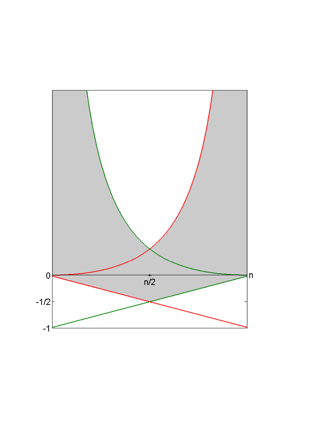
We illustrate by simulation results how the function of Definition 1.2 behaves when are defined by match lengths, as in Graph Model A of Definition 4.2. Note that since and , we know that and . See Figure 1 for a schematic illustration of the envelopes of these functions.
As Figure 1 might suggest, the function can take large positive values for close to or . However, since we are looking for the minimum value of , this does not affect the analysis. In Figure 2 we illustrate how behaves in a null model with no change-point. Observe that remains close to zero except at the end points, where it can take large positive values, as we would hope.
In Figure 3 we plot values of in a model formed by concatenating two IID sources in the sense of Definition 4.1. The change-point is marked by a vertical red line, and the function is minmised very close to this point, as we would hope. Further, in Figure 3, the form of the process observed fits closely with the theoretical properties of the corresponding process for generated by a toy model as in Section 5. Specifically, the function remains close to a piecewise smooth function, except close to the ends of the interval. Further, the piecewise smooth function is made up of three components; a concave function, a linear part, and another concave function. We explain how this pattern might be expected in Remark A.6 below.
We illustrate in Figure 4 how the algorithm performs over repeated trials simulated under Graph Model A. The histogram illustrates that the algorithm generally performs well, with a defined peak in estimates close to the true value . In particular, Figure 4 represents a solution to a difficult problem, in that it shows that our algorithm can efficiently partition a concatenation of a Markov chain with transition matrix with stationary distribution and an IID source with distribution . Methods based on crude symbol counts would fail here, but the algorithm essentially ‘discovers’ non-uniformity in the digram counts. The skewness of the histogram is perhaps to be expected, given the fact that Equations (37) and (39) below are not equal (these Equations bound the performance of the related toy Graph Model B).
Even when the two sources are not stationary, our estimator appears to detect the change-point accurately. That is, Figures 5 and 6 illustrate that our estimator accurately detects the change-point in models built up by concatenating natural language. In other words, in both figures, the function is minimised very close to the vertical line. The source of Figure 5 is formed by concatenating German and English versions of Faust, having sanitised the German text to remove umlauts, in order to make it look as English as possible. Figure 6 depicts a switch between two English authors.
Note that the value of is lower for Figure 5 than for Figure 6, illustrating the natural idea that two English authors are harder to distinguish than two authors writing in different languages. This fits with the simulation evidence provided in [13, Section V], where different languages, and different authors writing in English, are distinguished by relative entropy estimates. The authors suggest [13, Figures 15 and 17] that the relative entropy from English to German and from German to English are both around 2.5-2.6, whereas the relative entropy from one English author to another is typically around 0.3. However, note that the paper [13] considers a different situation, in that they consider a corpus of separate texts with authors already distinguished, whereas this paper shows how to partition a text by authorship.
7 Discussion
In this paper we have introduced a new change-point estimator, based on ideas from information theory. We have demonstrated that it works well for a variety of data sources, and proved -consistency in a related toy problem. We believe that the CRECHE can be adapted to detect change-points in a variety of related scenarios, and point out some directions for future research.
- 1.
First, we hope to prove consistency of under Graph Model A, by establishing a version of Theorem 1.3. This is likely to require an analysis of return times similar to those described in Section 3, taking into account the complicated dependencies that exist between return times of distinct and overlapping substrings. However, we regard Theorem 1.3 as a significant first step towards proving such a result, since the simulation results presented in this paper suggest that the estimator behaves similarly in both cases.
We note that, under Graph Model A, we expect the rate of convergence of to to be quicker than the obtained in Theorem A.1, and perhaps even comparable with the obtained by [10]. This is because a joint version of the Asymptotic Equipartition Property suggests that a typical string of length from will have -probability decaying like for a certain constant. This suggests that in terms of the toy model, we should consider crossing probabilities and decaying to 0. Remark A.7 below shows that in the case , much faster convergence is achieved in the toy model.
- 2.
Second, we believe that these consistency results should extend to scenarios with multiple change-points (assuming the number of change-points is low compared to the length of the data stream). In this case, simulations show that should have several local minima, each corresponding to a change-point, but the analysis required to prove this is more involved.
- 3.
Third, we believe that estimators of CRECHE type can be extended to real-valued data, as opposed to those coming from finite alphabets. In this setting, we should be able to construct a directed graph using closest matchings in Euclidean distance, motivated by ideas from rate-distortion theory. We can then use the crossings function in precisely the same way.
- 4.
Finally, in future work we will address the issue of quickest detection of change-points in streaming data, in the spirit of [40]. By estimating the typical set during the burn-in period, we believe that match lengths can act as a proxy for the log-likelihood in the CUSUM test.
Appendix A Proof of Theorem 1.3
A.1 Matchings in an IID setting
First, we consider the behaviour of the crossings function in a simpler situation than the Graph Model B of Definition 5.1, by considering a model without a change-point, analogous to Figure 2. We obtain uniform control of the type required.
Theorem A.1.
For each define independently uniformly distributed on . For the normalized crossings process of Definition 1.2, for any and ,
| (13) |
that is, is a pathwise confidence region on the process.
The control of provided by Theorem A.1 is of optimal order, in the following two senses:
Remark A.2.
Remark A.2 helps to explain the large fluctuations in seen in Figure 2. In this toy model with no change-point: for , the maximal fluctuations of are , but for , the maximal fluctuations are . Similarly, fluctuations in will be for bounded away from zero, and overall.
We first prove a technical lemma regarding the thinning operation introduced by Rényi [42]. That is, for each random variable , the -thinned version , where are Bernoulli(), independent of each other and of . This allows us to describe a process with binomial marginals which will prove useful for us. In the language of [5] this process is a (non-stationary) first-order integer-valued autoregressive process, a discrete equivalent of an AR(1) time series process.
Lemma A.3.
For fixed and , define a process by , and recursively taking
| (16) |
where independently of all other random variables. Then,
- 1.
For all , the .
- 2.
The process is a martingale.
- 3.
For any , the process is a martingale.
Proof.
- 1.
Note that this result is true by definition for , we will prove it by induction in general. Recall that for any , and , if then . Assuming for a particular , then
- 2.
This means that for all . As a result, since
and since exactly when :
by substituting for .
- 3.
Write , , and . By a similar argument, since when say, we know that
since and .
∎
Proof of Theorem A.1.
The key is to observe that for uniform on , . This means that the LR crossing process is a Markov (birth and death) process. If we know that , then the links that cross will cross independently with probability . In addition, there will be a contribution due to .
In other words, the process is distributed exactly as in Lemma A.3, with and . This means that by Lemma A.3, is a martingale. By a standard argument (see for example [50, Section 14.6]), since is a martingale, Jensen’s inequality implies that is a submartingale. Doob’s submartingale inequality [50, Section 14.6] states that for any non-negative submartingale , for any and :
| (17) |
Since , the , so we know that .
Hence, taking , and in Equation (17), the theorem follows. ∎
A.2 Matching in a change-point setting
We now use the insights of Appendix A.1 to control the behaviour of the crossings process for Graph Model B, where a change-point is present at . First we use Lemma A.3 to deduce that:
Proposition A.4.
The process defined by
is a martingale. Here mean functions
| (21) | |||||
| (22) |
Further equals
| for , | (23) | ||||
| for . | (24) |
Proof.
The key is to observe that, under Graph Model B, for :
| (25) |
and for , the for . This means that
- 1.
For , the . We deduce that is a martingale in this range and that by applying Lemma A.3 with and . We deduce the variance of since .
- 2.
For , we divide , where and . As before
- (a)
. In this case, since
we can divide by to deduce that is a martingale. Further, .
- (b)
. In this case, by considering (since if then ) we can write . This means we can apply Lemma A.3 with and , to deduce that is a martingale. As before .
The fact that is a martingale follows since the sum of two independent martingales is a martingale. We deduce the mean and variance of since .
- (a)
∎
Using this martingale characterization, and Doob’s submartingale inequality Equation (17), we can control uniformly, as before. This allows us to control , as illustrated in Figure 7. Essentially, the confidence regions for are tilted versions of the confidence region of Theorem A.1. This means that the stay close to their mean functions for , so that the minimum of must be close to the minimum of the mean functions, namely . This is illustrated in Figure 7.
Remark A.5.
By symmetry, the process defined by
is a time-reversed martingale. Here we write
| (29) | |||||
| (30) |
For the corresponding , the
| (31) |
Remark A.6.
Note that the form of and helps explain the form of the process seen in Figures 3 and 7. That is, Equations (21) and (22) show that the mean of is made up of a concave part left of the change-point and a linear part right of the change-point. Similarly by Equations (29) and (30), the mean of will have a linear part left of the change-point and a concave part right of the change-point.
Notice that the curve made up of for and for is minimised at with value . Similarly is minimised at with value .
In the proof of Theorem 1.3 we need to distinguish two cases, according to which of and is smaller. We briefly remark that in the symmetric case , that if and only if . Further, in the limiting case , the two curves and intersect at .
Proof of Theorem 1.3.
Without loss of generality, we will assume that , and pick . Further we assume , which is true if .
First, we observe that the curve cannot be minimised too close to either end of the interval of interest. We write . Recall that (see Figure 1) and . This means that for we know that , and for we know that .
This means that we can use the union bound and standard conditioning arguments to decompose the error probability into three terms:
| (32) | |||||
| (33) | |||||
| (34) | |||||
using the fact that . We can bound each of these terms in order.
- 1.
- 2.
To bound (33), the key is to observe that the mean term defined in Equation (21) is a concave function. This means that for we know that
(36) As defined in Proposition A.4, is a multiple of with a coefficient which decreases in , so for , we can bound it by This means that by Equations (21) and (36)
(37) - 3.
The result follows on adding together the contributions from Equations (35), (37) and (39). We can choose for example , since , since the assumption that ensures that . Putting these terms together, we deduce that we can take
| (40) | |||||
∎
Remark A.7.
Note that the form of (40) suggests that as tends to zero, then will tend to infinity, meaning that this is the hardest case. Of course, the case will have no crossings of , so should be the easiest case. We can indeed do much better by adapting the argument slightly. Without loss of generality assume that , and recall that in this case , and we can choose , so that . This means that Equations (32) and (33) are zero, since , and since the interval is empty. Then taking in Equation (39) gives . Overall, this means that
suggesting that the estimator is -consistent in this case.
In fact, we can do better. Since the interval is empty, we can strengthen the bound on (33) to deduce that . Further notice that when , the , since the interval is again empty.
Otherwise, we divide the interval into further subintervals, using a similar argument to that used to obtain (39). Since Equation (24) gives , for any we know that
| (41) | |||||
This means that we can pick a constant , and divide the interval into subintervals , where and , where , with . Applying the union bound to these intervals, we deduce by Equation (41) that
| (42) |
or in other words that the probability that the estimator makes a mistake is . Up to the factor of , this probability is of optimal order, since for independence implies that
as and .
Acknowledgements
This work was funded by a grant from the Ministry of Defence, via the Underpinning Defence Mathematics programme. We would like to thank Christophe Andrieu of Bristol University and Tim Boxer of the Industrial Mathematics KTN for their support and advice.
References
- [1] M. Abadi and A. Galves. A version of Maurer’s conjecture for stationary -mixing processes. Nonlinearity, 17(4):1357–1366, 2004.
- [2] R. Aggarwal, C. Inclan, and R. Leal. Volatility in emerging stock markets. The Journal of Financial and Quantitative Analysis, 34(1):33–55, 1999.
- [3] D. J. Aldous and P. C. Shields. A diffusion limit for a class of randomly-growing binary trees. Probab. Theory Related Fields, 79(4):509–542, 1988.
- [4] P. H. Algoet and T. M. Cover. A sandwich proof of the Shannon-McMillan-Breiman theorem. Ann. Probab., 16:899–909, 1988.
- [5] A. A. Alzaid and M. Al-Osh. An integer-valued th-order autoregressive structure () process. Journal of Applied Probability, 27(2):314–324, 1990.
- [6] R. Arratia and M. S. Waterman. Critical phenomena in sequence matching. Ann. Probab., 13(4):1236–1249, 1985.
- [7] R. Arratia and M. S. Waterman. The Erdős-Rényi strong law for pattern matching with a given proportion of mismatches. Ann. Probab., 17(3):1152–1169, 1989.
- [8] T. P. Barnett, D. W. Pierce, and R. Schnur. Detection of anthropogenic climate change in the world’s oceans. Science, 292(5515):270–274, 2001.
- [9] C. Bell, L. Gordon, and M. Pollak. An efficient nonparametric detection scheme and its application to surveillance of a Bernoulli process with unknown baseline. Lecture Notes-Monograph Series, 23:7–27, 1994.
- [10] S. Ben Hariz, J. J. Wylie, and Q. Zhang. Optimal rate of convergence for nonparametric change-point estimators for nonstationary sequences. Ann. Statist., 35(4):1802–1826, 2007.
- [11] J. V. Braun, R. K. Braun, and H. G. Muller. Multiple changepoint fitting via quasilikelihood, with application to DNA sequence segmentation. Biometrika, 87(2):301–314, 2000.
- [12] B. E. Brodsky and B. S. Darkhovsky. Nonparametric methods in change-point problems, volume 243 of Mathematics and its Applications. Kluwer Academic Publishers Group, Dordrecht, 1993.
- [13] H. Cai, S. R. Kulkarni, and S. Verdú. Universal divergence estimation for finite-alphabet sources. IEEE Trans. Inform. Theory, 52(8):3456–3475, 2006.
- [14] E. Carlstein. Nonparametric change-point estimation. The Annals of Statistics, 16(1):188–197, 1988.
- [15] T. M. Cover and J. A. Thomas. Elements of Information Theory. John Wiley, New York, 1991.
- [16] R. W. R. Darling. Fluid limits of pure jump Markov processes: a practical guide. see arXiv:math/0210109, 2002.
- [17] R. M. Dudley. Real analysis and probability. Wadsworth & Brooks/Cole Advanced Books & Software, Pacific Grove, CA, 1989.
- [18] L. Dümbgen. The asymptotic behavior of some nonparametric change-point estimators. Ann. Statist., 19(3):1471–1495, 1991.
- [19] M. Frisén and J. D. Maré. Optimal surveillance. Biometrika, 78(2):271–280, 1991.
- [20] Y. Gao, I. Kontoyiannis, and E. Bienenstock. Estimating the entropy of binary time series: methodology, some theory and a simulation study. Entropy, 10(2):71–99, 2008.
- [21] J. Girón, J. Ginebra, and A. Riba. Bayesian analysis of a multinomial sequence and homogeneity of literary style. The American Statistician, 59(1):19–30, 2005.
- [22] A. Goldenshluger, A. Tsybakov, and A. Zeevi. Optimal change-point estimation from indirect observations. Ann. Statist., 34(1):350–372, 2006.
- [23] L. Gordon and M. Pollak. An efficient sequential nonparametric scheme for detecting a change of distribution. The Annals of Statistics, 22(2):763–804, 1994.
- [24] P. Grassberger. Estimating the information content of symbol sequences and efficient codes. IEEE Trans. Information Theory, 35:669–675, 1989.
- [25] L. Horváth. The maximum likelihood method for testing changes in the parameters of normal observations. The Annals of Statistics, 21(2):671–680, 1993.
- [26] P. Jacquet and W. Szpankowski. Asymptotic behavior of the Lempel-Ziv parsing scheme and in digital search trees. Theoret. Comput. Sci., 144(1-2):161–197, 1995.
- [27] O. T. Johnson. A Central Limit Theorem for non-overlapping return times. Journal of Applied Probability, 43(1):32–47, 2006.
- [28] M. Kac. On the notion of recurrence in discrete stochastic processes. Bull. Amer. Math. Soc., 53:1002–1010, 1947.
- [29] R. Killick, P. Fearnhead, and I. A. Eckley. Optimal detection of changepoints with a linear computational cost. see arXiv:1101.1438, 2011.
- [30] D. H. Kim. The recurrence of blocks for Bernoulli processes. Osaka J. Math., 40(1):171–186, 2003.
- [31] H. Kim, B. L. Rozovskii, and A. G. Tartakovsky. A nonparametric multichart CUSUM test for rapid detection of DOS attacks in computer networks. International Journal of Computing and Information Sciences, 2(3):149–158, 2004.
- [32] A. N. Kolmogorov. Sulla determinazione empirica di una legge di distribuzione. Inst. Ital. Atti. Giorn., 4:83–91, 1933.
- [33] I. Kontoyiannis. Asymptotic recurrence and waiting times for stationary processes. J. Theoret. Probab., 11(3):795–811, 1998.
- [34] I. Kontoyiannis and Y. M. Suhov. Prefixes and the entropy rate for long-range sources. In F. P. Kelly, editor, Probability, Statistics and Optimisation, pages 89–98. John Wiley, New York, 1993.
- [35] U. M. Maurer. A universal statistical test for random bit generators. J. Cryptology, 5(2):89–105, 1992.
- [36] X. Nguyen, M. Wainwright, and M. Jordan. Nonparametric decentralized detection using kernel methods. IEEE Transactions on Signal Processing, 53(11):4053 – 4066, 2005.
- [37] D. S. Ornstein and B. Weiss. How sampling reveals a process. Ann. Probab., 18:905–930, 1990.
- [38] D. S. Ornstein and B. Weiss. Entropy and data compression schemes. IEEE Trans. Information Theory, 39:78–83, 1993.
- [39] M. Pollak. Optimal detection of a change in distribution. The Annals of Statistics, 13(1):206–227, 1985.
- [40] H. V. Poor and O. Hadjiliadis. Quickest detection. Cambridge University Press, Cambridge, 2009.
- [41] A. N. Quas. An entropy estimator for a class of infinite processes. Theory Probab. Appl., 43(3):496–507, 1999.
- [42] A. Rényi. A characterization of Poisson processes. Magyar Tud. Akad. Mat. Kutató Int. Közl., 1:519–527, 1956.
- [43] A. Riba and J. Ginebra. Change-point estimation in a multinomial sequence and homogeneity of literary style. Journal of Applied Statistics, 32(1):61–74, 2005.
- [44] A. J. Scott and M. Knott. A cluster analysis method for grouping means in the analysis of variance. Biometrics, 30(3):507–512, 1974.
- [45] P. C. Shields. Entropy and prefixes. Ann. Probab., 20:403–409, 1992.
- [46] P. C. Shields. The ergodic theory of discrete sample paths. American Mathematical Society, Providence, RI, 1996.
- [47] P. C. Shields. String matching bounds via coding. Ann. Probab., 25:329–336, 1997.
- [48] G. R. Shorack and J. A. Wellner. Empirical processes with applications to statistics. John Wiley & Sons Inc., New York, 1986.
- [49] J. A. Wellner. A martingale inequality for the empirical process. The Annals of Probability, 5(2):303–308, 1977.
- [50] D. Williams. Probability with Martingales. Cambridge University Press, Cambridge, 1991.
- [51] A. J. Wyner. String matching theorems and applications to data compression and statistics. PhD thesis, Stanford University, 1993.
- [52] A. J. Wyner. More on recurrence and waiting times. Ann. Appl. Probab., 9(3):780–796, 1999.
- [53] J. Ziv and A. Lempel. A universal algorithm for sequential data compression. IEEE Trans. Information Theory, 23:337–343, 1977.
- [54] J. Ziv and A. Lempel. Compression of individual sequences via variable rate coding. IEEE Trans. Information Theory, 24:530–536, 1978.
- [55] J. Ziv and N. Merhav. A measure of relative entropy between individual sequences with application to universal classification. IEEE Trans. Inform. Theory, 39(4):1270 –1279, 1993.