跳到论文正文
W Papers独立论文阅读器 arXiv:1106.5367 论文正文 计算阅读时间 · 0%
引用这篇论文根据当前论文元数据生成,正式投稿前建议核对。


License: arXiv.org perpetual non-exclusive license
arXiv:1106.5367v1 [cs.IT] 27 Jun 2011

Partial Interference Alignment for KK-user MIMO Interference ChannelsThanks: The authors are with the Department of Electronic and Computer Engineering (ECE), Hong Kong University of Science and Technology (HKUST), Hong Kong.

Huang Huang, Student Member, IEEE, Vincent K. N. Lau, Senior Member, IEEE Affiliation: 
Abstract

In this paper, we consider a Partial Interference Alignment and Interference Detection (PIAID) design for KK-user quasi-static MIMO interference channels with discrete constellation inputs. Each transmitter has MM antennas and transmits LL independent data streams to the desired receiver with NN receive antennas. We focus on the case where not all K−1K-1 interfering transmitters can be aligned at every receiver. As a result, there will be residual interference at each receiver that cannot be aligned. Each receiver detects and cancels the residual interference based on the constellation map. However, there is a window of unfavorable interference profile at the receiver for Interference Detection (ID). In this paper, we propose a low complexity Partial Interference Alignment scheme in which we dynamically select the user set for IA so as to create a favorable interference profile for ID at each receiver. We first derive the average symbol error rate (SER) by taking into account of the non-Guassian residual interference due to discrete constellation. Using graph theory, we then devise a low complexity user set selection algorithm for the PIAID scheme, which minimizes the asymptotically tight bound for the average end-to-end SER performance. Moreover, we substantially simplify interference detection at the receiver using Semi-Definite Relaxation (SDR) techniques. It is shown that the SER performance of the proposed PIAID scheme has significant gain compared with various conventional baseline solutions.

I Introduction

Interference has been a very difficult problem in wireless communications.. For instance, the capacity region of two-user Gaussian interference channels has been an open problem for over 30 years [1]. Recently, there are some progress made in understanding the interference [2, 3] and extensive studies have been done regarding the Interference Alignment (IA) [3]. For instance, IA is a signal processing approach that attempts to simultaneously align the interference on a lower dimension subspace at each receiver so that the desired signals can be transmitted on the interference-free dimensions. In [4], the authors show that IA (using infinite dimension symbol extension in time or frequency selective fading channels) is optimal in Degrees-of-Freedom (DoF) sense. In [5] the authors propose a variation of the IA scheme, the ergodic alignment scheme, for KK-user time or frequency-selective interference channels. In practice, since it is not possible to realize infinite dimension symbol extensions, there are a number of works [6, 7, 8] and the reference therein that consider IA in the spatial domain, without symbol extensions, in the KK-user quasi-static MIMO interference channels. Furthermore, the authors in [9] investigate the asymptotic performance of these different IA solutions. However, for quasi-static (or constant) channels, conventional IA might be infeasible depending on the system parameters. For example, it is conjectured in [10] that conventional IA on quasi-static MIMO (MM transmit and NN receive antennas) interference channels is not feasible to achieve a per user DoF greater than M+NK+1\frac{M+N}{K+1}. As a result, we cannot rely on IA to eliminate all interference in quasi-static MIMO interference channels especially when KK is large. There are other works that consider IA over signal scale in [11, 12, 13, 14]. In [11] and [12], signal scale alignment schemes are introduced for the many-to-one interference channel and fully connected interference networks, respectively. In [13, 14], the authors propose a lattice alignment scheme for KK-user MIMO interference channels. However, the scheme requires infinite SNR and serves only as a proof of concept. It is not clear whether this approach can be applied at finite SNR.

Due to the fact that not all the interferers can be aligned at each receiver, there will be residual interference at the receiver. In this paper, we assume the receiver has interference detection (ID) capability. Specifically, the receiver detects and cancels the residual interference based on the constellation map derived from the discrete constellation inputs. However, there is a window of unfavorable interference profile for ID at the receiver. For instance, ID at the receiver is more effective when the interference is stronger than the desired signal [15, 14]. In [15, 16], the authors propose an ID scheme for quasi-static interference channels based on lattices. However the proposed scheme can only work under idealized assumptions such as the symmetric SISO interference channels (where all cross links have the same fading coefficients) or a specialized class of 3-user SISO interference channels (where the product of fading coefficients is assumed to be rational).

In fact, IA and ID are complementary approaches to deal with interference in quasi-static MIMO interference channels. The IA approach11 1 In the remaining papers, the mentioned IA approach specifically refers to the signal space alignment approach. can be used to first eliminate some interference and the ID approach can be used to deal with the residual interference at each receiver. While we can potentially benefit from the concepts of IA and ID approaches in dealing with interference, there are still some key technical challenges to be addressed.

  • •

    Feasibility Issue of IA and Path Loss Effects: Sometimes brute-force IA in quasi-static MIMO interference channels (without symbol extensions) might be infeasible depending on system parameters. Furthermore, existing literature has completely ignored the effects of path loss, which may also be exploited when dealing with interference. For instance, nodes with large path loss may not need to be interference-aligned and hence, it is important to jointly consider the feasibility issue and the path loss effects.

  • •

    Coupling between IA and ID: While both IA and ID are effective means to mitigate interference, their designs are coupled together in an intricate manner. For instance, the performance of ID at the receiver depends heavily on the interference profile. Hence, IA can potentially contribute to creating a more desirable interference profile for ID by careful selecting a subset of users for IA. However, the problem of user selection in IA to optimize the symbol error rate (SER) performance is very complicated. First, the optimization space is combinatorial and brute force exhaustive search is not viable. Second, even if we can afford the search complexity, obtaining the search metric is highly non-trivial because it is also very challenging to analyze the closed form average SER under non-Gaussian interferences.

In this paper, we propose a low complexity Partial Interference Alignment and Interference Detection (PIAID) scheme for KK-user quasi-static MIMO interference channels with discrete constellation inputs. We consider QPSK constellations22 2 QPSK constellations are easier to analyze. However, the proposed framework can be extended to QAM constellations easily. at the inputs of the KK transmitters and each transmit-receive pair may have different path losses. The proposed PIAID scheme dynamically selects the interference alignment set at each receiver based on the path loss information to create a favorable interference profile at each receiver for ID processing as illustrated in Fig. 2. Interference alignment is applied only to the members of the alignment set. We derive the average SER by taking into account the non-Guassian residual interference due to discrete constellation. Using graph theory, we transform the combinatorial problem into a linear programming (LP) problem and obtain a low complexity user set selection algorithm for the PIAID scheme, which minimizes the asymptotically tight bound for the average end-to-end SER performance. Furthermore, using Semi-Definite Relaxation (SDR) technique [17, 18, 19, 20], we propose a low complexity ID algorithm at the receiver. The SER performance of the proposed PIAID scheme is shown to have significant gain compared with various conventional baseline solutions.

Outline: The rest of this paper is organized as follows. In Section II, we outline the system model and the proposed PIAID scheme. In Section III, we discuss the optimization of the IA user selection. In Section IV, we derive the average SER by taking into account the non-Guassian residual interference and propose a low complexity ID algorithm at the receiver that uses SDR technique. The numerical simulation results are illustrated in Section V. Finally we conclude with a brief summary in Section VI.

II System Model

II-A KK-user Quasi-Static MIMO Interference Channels

We consider KK-user quasi-static MIMO Gaussian interference channels as illustrated in Fig. 1. Specifically, each MM-antenna transmitter, tries to communicate to its corresponding NN-antenna receiver. The channel output at the kk-th receive node is described as follows:

𝐲k=∑i∈𝒦Pi​Lk​i​𝐇k​i​𝐱¯i+𝐳k,\mathbf{y}_{k}=\sum_{i\in\mathcal{K}}\sqrt{P_{i}L_{ki}}\mathbf{H}_{ki}\mathbf{\overline{x}}_{i}+\mathbf{z}_{k}, (1)

where 𝒦={1,⋯,K}\mathcal{K}=\{1,\cdots,K\}, 𝐇k​i∈ℂN×M\mathbf{H}_{ki}\in\mathbb{C}^{N\times M} is the MIMO complex fading coefficients from the ii-th transmitter to the kk-th receiver, Lk​iL_{ki} is the long term path gain from the ii-th transmitter to the kk-th receiver, and PiP_{i} is the average transmit power of the ii-th transmitter. In (1), 𝐱¯i∈ℂM×1\mathbf{\overline{x}}_{i}\in\mathbb{C}^{M\times 1} is the complex signal vector transmitted by transmit node ii, and 𝐳k∈ℂN×1\mathbf{z}_{k}\in\mathbb{C}^{N\times 1} is the circularly symmetric Additive White Gaussian Noise (AWGN) vector at receive node kk. We assume all noise terms are i.i.d zero mean complex Gaussian with 𝔼⁡[𝐳k​(𝐳k)H]=2​𝐈N\mathbb{E}[\mathbf{z}_{k}(\mathbf{z}_{k})^{H}]=2\mathbf{I}_{N}. Furthermore, the assumption on channel model is given as follows:

Assumption 1 (Assumption on Channel Model [21])

We assume that the long term path gain is given by Lk​i=ω​dk​i−γL_{ki}=\omega d_{ki}^{-\gamma}, where dk​id_{ki} is the distance between transmit node ii and receive node kk, ω\omega is the Log-normal shadow fading with a standard deviation σω\sigma_{\omega}, and γ\gamma is the path loss exponent. Furthermore, we assume that the entries of 𝐇k​i\mathbf{H}_{ki} for all k,ik,i are i.i.d. complex Gaussian random variables given by [𝐇k​i](n,m)∼𝒞​𝒩​(0,1)[\mathbf{H}_{ki}]_{(n,m)}\sim\mathcal{CN}(0,1) for all k,i,n,mk,i,n,m, where [𝐇k​i](n,m)[\mathbf{H}_{ki}]_{(n,m)} denotes the (n,m)th(n,m)^{\text{th}} element of 𝐇k​i\mathbf{H}_{ki}.   ∎

In this paper, we assume that the ii-th transmit node transmits D≤min⁡(M,N)D\leq\min(M,N) independent QPSK data streams {xi1,⋯,xiD}\{x_{i}^{1},\cdots,x_{i}^{D}\} to the ii-th receive node where xid∈𝒮={22​(1+j),22​(1−j),22​(−1+j),22​(−1−j)},∀d∈{1,⋯,D}x_{i}^{d}\in\mathcal{S}=\{\frac{\sqrt{2}}{2}(1+j),\frac{\sqrt{2}}{2}(1-j),\frac{\sqrt{2}}{2}(-1+j),\frac{\sqrt{2}}{2}(-1-j)\},\forall d\in\{1,\cdots,D\}. Let 𝐯id\mathbf{v}_{i}^{d} (‖𝐯id‖=1||\mathbf{v}_{i}^{d}||=1, where ||⋅||||\cdot|| denotes the Frobenius norm.) denote the precoder for the xidx_{i}^{d} symbol. Hence, the transmitted vector at the ii-th transmitter is given by 𝐱¯i=∑d𝐯id​xid\mathbf{\overline{x}}_{i}=\sum_{d}\mathbf{v}_{i}^{d}x_{i}^{d}.

II-B Partial Interference Alignment and Interference Detection (PIAID) Scheme

The proposed PIAID scheme consists of two major components, namely the Partial Interference Alignment (PIA) at the transmitters and the Interference Detection (ID) at the receivers as illustrated in Fig. 2.

II-B1 Overview of PIA

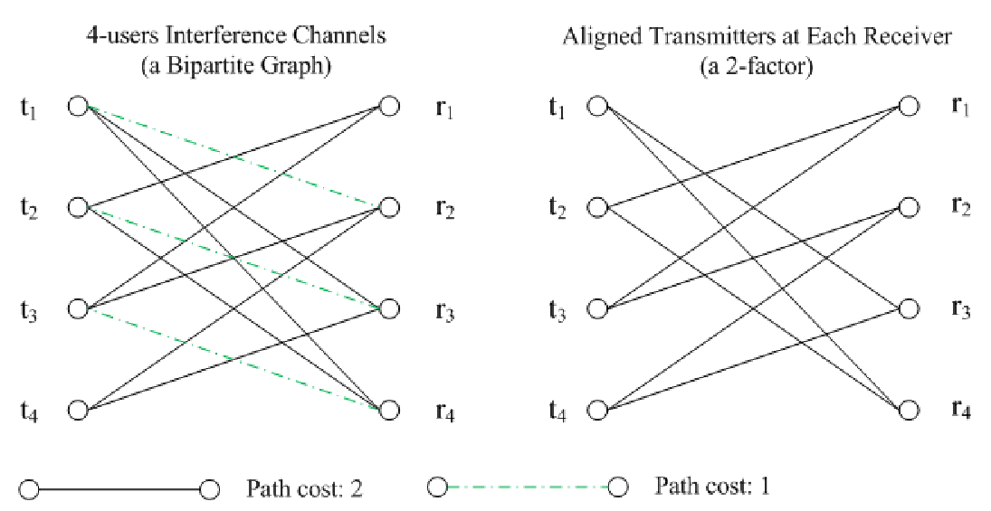
PIA is motivated by the feasibility issue33 3 For constant MIMO interference channels, it is not always possible to completely align all the K−1K-1 interferers at each receiver. of the MIMO interference alignment without symbol extension [10, 6]. For instance, it is conjectured in [10] that only when K≤M+ND−1K\leq\frac{M+N}{D}-1, the K−1K-1 interfering transmitters can be aligned at every receiver node. As a result, not all the K−1K-1 interfering transmitters can be aligned at every receiver node for large KK. Furthermore, existing IA schemes do not consider or exploit the effects of different path losses between transmit and receive pairs. When the path loss effects are taken into consideration, not all transmitters will contribute the same effect at the receiver and hence, there should be different priority in determining which nodes should be aligned given the feasibility constraint. Fig. 3 illustrates an example of 4-user interference channels where M=N=2M=N=2 and D=1D=1. Using the feasibility condition of MIMO IA in [10], only two transmitters can be aligned at each receiver. Combining with the path costs (which depend on the path gains and transmit power), it is obvious that transmitters 2 and 3 should be aligned at receiver 1 as indicated in the Fig. 3.

Motivated by the above example, the proposed PIAID scheme dynamically selects α\alpha transmitters to be aligned at each receiver node based on the path costs. The index of the aligned transmitters at each receiver is given by a PIA set with cardinality α\alpha. Specifically, the PIA set is defined below.

Definition 1 (PIA Set)

A PIA set is defined as 𝒜={𝒜k,∀k}\mathcal{A}=\{\mathcal{A}_{k},\forall k\}, where 𝒜k={k1,k2,⋯,kα≠k}\mathcal{A}_{k}=\{k_{1},k_{2},\cdots,k_{\alpha}\neq k\} denotes the index of aligned transmitters at the receiver kk for some constant α\alpha.   ∎

Only the transmit nodes that belong to 𝒜k\mathcal{A}_{k} will have to align their transmit signals by choosing the precoders and equalizers according to the traditional IA requirement44 4 Note that the requirement is equivalent to that used in [10, 22], i.e., choosing the precoders and equalizers satisfying rank​((𝐔k)†​𝐇k​k​𝐕k)=D,∀k\text{rank}((\mathbf{U}_{k})^{{\dagger}}\mathbf{H}_{kk}\mathbf{V}_{k})=D,\forall k. [10, 22]

(𝐔k)†​𝐇k​i​𝐕i\displaystyle(\mathbf{U}_{k})^{{\dagger}}\mathbf{H}_{ki}\mathbf{V}_{i} =\displaystyle= 𝟎,∀i∈𝒜k\displaystyle\mathbf{0},\forall i\in\mathcal{A}_{k}
(𝐔k)†​𝐇k​k​𝐕k\displaystyle(\mathbf{U}_{k})^{{\dagger}}\mathbf{H}_{kk}\mathbf{V}_{k} =\displaystyle= diag​(λ1,⋯,λD),∀k\displaystyle\text{diag}(\lambda_{1},\cdots,\lambda_{D}),\forall k (2)

where (⋅)†(\cdot)^{\dagger} denotes the Hermitian transpose, diag​(λ1,⋯,λD)\text{diag}(\lambda_{1},\cdots,\lambda_{D}) denotes a diagonal matrix with diagonal entries λ1,⋯,λD\lambda_{1},\cdots,\lambda_{D}, 𝐔k=[𝐮k1,⋯,𝐮kD]\mathbf{U}_{k}=[\mathbf{u}_{k}^{1},\cdots,\mathbf{u}_{k}^{D}] are the N×DN\times D decorrelators at receiver kk with ‖𝐮kl‖=1,∀l||\mathbf{u}_{k}^{l}||=1,\forall l, and 𝐕i=[𝐯i1,⋯,𝐯iD]\mathbf{V}_{i}=[\mathbf{v}_{i}^{1},\cdots,\mathbf{v}_{i}^{D}] are the M×DM\times D precoders at transmitter ii with ‖𝐯il‖=1,∀l||\mathbf{v}_{i}^{l}||=1,\forall l. Based on the conjecture in [10], a sufficient condition55 5 From [10], we know that the total number of equations for the IA requirement {(𝐔k)†𝐇k​i𝐕i=𝟎,∀i∈𝒜k,∀k}\{(\mathbf{U}_{k})^{{\dagger}}\mathbf{H}_{ki}\mathbf{V}_{i}=\mathbf{0},\forall i\in\mathcal{A}_{k},\forall k\} is Ne=∑k|𝒜k|​D2=α​K​D2N_{e}=\sum_{k}|\mathcal{A}_{k}|D^{2}=\alpha KD^{2}, and the total number of variables is Nv=∑kD⁡(M+N−2​D)=K​D​(M+N−2​D)N_{v}=\sum_{k}D(M+N-2D)=KD(M+N-2D). When each transmitter is selected by α\alpha receivers, the feasibility condition is simply given by Ne≤NvN_{e}\leq N_{v} [10], i.e., α⁡(𝒜)≤min⁡(M+ND−2,K−1)\alpha(\mathcal{A})\leq\min\left(\frac{M+N}{D}-2,K-1\right). for a feasible PIA set 𝒜\mathcal{A} is given by[10]:

α(𝒜)≤min(M+ND−2,K−1) and ∑k𝟏(i∈𝒜k)=α(𝒜),∀i\alpha(\mathcal{A})\leq\min\left(\frac{M+N}{D}-2,K-1\right)\text{ and }\sum\nolimits_{k}\mathbf{1}(i\in\mathcal{A}_{k})=\alpha(\mathcal{A}),\forall i (3)

where 𝟏​(⋅)\mathbf{1}(\cdot) is the indicator function, α⁡(𝒜)=|𝒜k|\alpha(\mathcal{A})=|\mathcal{A}_{k}| is the cardinality of 𝒜k\mathcal{A}_{k} (i.e., the number of aligned interferers at each receiver). The requirement as per (3) means that each transmitter should be selected by α⁡(𝒜)\alpha(\mathcal{A}) receivers. The IA set 𝒜\mathcal{A} is a design parameter in the proposed PIA scheme, and how to choose the IA set is presented in Section III.

Remark 1 (Feasibility Condition)

Note that the feasibility conditions for (2) are still open in the literature. Since the feasibility condition and computation of {𝐔k,𝐕k,∀k}\{\mathbf{U}_{k},\mathbf{V}_{k},\forall k\} are not the focus of the paper, we have adopted the results in [10] to derive a sufficient condition (3). While this condition restricts the choice of the feasible set 𝒜\mathcal{A}, it introduces graph structure for the optimization w.r.t. 𝒜\mathcal{A}. Furthermore, as shown in Fig. 6, the proposed PIA algorithm with condition (3) has similar performance as the solution obtained by brute-force exhaustive search (without (3)).   ∎

II-B2 Overview of ID

In this paper, we focus on the case where not all the K−1K-1 interferers can be aligned at each receivers. As a result, there will be residual interference at every receiver. The ID processing at the receiver first estimates the aggregate interference signal by using the constellation maps derived from the QPSK inputs. The desired signal is detected after subtracting the estimated aggregate interference. For instance, the normalized received signal at the kk-th receiver is given by:

𝐲k=Pk​Lk​k𝐇k​k𝐯klxkl+∑d≠lPk​Lk​k​𝐇k​k​𝐯kd​xkd⏟inter-stream interference+∑i∉𝒜k;dPi​Lk​i​𝐇k​i​𝐯id​xid⏟non-aligned interferers+∑i∈𝒜k;dPi​Lk​i​𝐇k​i​𝐯id​xid⏟aligned interferers+𝐳k.\begin{array}[]{ll}&\mathbf{y}_{k}=\sqrt{P_{k}L_{kk}}\mathbf{H}_{kk}\mathbf{v}_{k}^{l}x_{k}^{l}+\underbrace{\sum\nolimits_{d\neq l}\sqrt{P_{k}L_{kk}}\mathbf{H}_{kk}\mathbf{v}_{k}^{d}x_{k}^{d}}_{\text{inter-stream interference}}\\ &\quad\quad\quad\quad+\underbrace{\sum\nolimits_{i\not\in\mathcal{A}_{k};d}\sqrt{P_{i}L_{ki}}\mathbf{H}_{ki}\mathbf{v}_{i}^{d}x_{i}^{d}}_{\text{non-aligned interferers}}+\underbrace{\sum\nolimits_{i\in\mathcal{A}_{k};d}\sqrt{P_{i}L_{ki}}\mathbf{H}_{ki}\mathbf{v}_{i}^{d}x_{i}^{d}}_{\text{aligned interferers}}+\mathbf{z}_{k}.\end{array} (4)

We adopt linear processing at the receiver and the detection process for ll-th data stream at the kk-th receiver is divided into two stages, namely the aggregate interference detection stage (stage I) and the desired signal detection stage (stage II). The two stages are elaborated below:

  • •

    Stage I Processing: Using the ll-th column of 𝐔k\mathbf{U}_{k} in (2), 𝐮kl\mathbf{u}_{k}^{l}, as the decorrelator, the post-processed signal of the ll-th stream is given by:

    ykl=(𝐮kl)†𝐲k=Pk​Lk​kHk​kl​lxkl+∑i∉𝒜k;dPi​Lk​i​Hk​il​d​xid⏟non-aligned interferers+(𝐮kl)†𝐳k,\displaystyle y_{k}^{l}=(\mathbf{u}_{k}^{l})^{{\dagger}}\mathbf{y}_{k}=\sqrt{P_{k}L_{kk}}H_{kk}^{ll}x_{k}^{l}+\underbrace{\sum_{i\not\in\mathcal{A}_{k};d}\sqrt{P_{i}L_{ki}}H_{ki}^{ld}x_{i}^{d}}_{\text{non-aligned interferers}}+(\mathbf{u}_{k}^{l})^{{\dagger}}\mathbf{z}_{k}, (5)

    where Hk​il​d=(𝐮kl)†​𝐇k​i​𝐯idH_{ki}^{ld}=(\mathbf{u}_{k}^{l})^{{\dagger}}\mathbf{H}_{ki}\mathbf{v}_{i}^{d} is the equivalent channel gain for the dd-th data stream of transmitter ii at receiver kk. Note that the inter-stream interference and the interference contributed by users in the IA set 𝒜k\mathcal{A}_{k} are completely eliminated due to the PIA requirement in (2). Let 𝒬k={i:PiLk​i≥PkLk​k,∀i∉𝒜k,i≠k}⊆{1,⋯,K}\mathcal{Q}_{k}=\{i:P_{i}L_{ki}\geq P_{k}L_{kk},\forall i\not\in\mathcal{A}_{k},i\neq k\}\subseteq\{1,\cdots,K\} denotes the set of strong residual interference. Since ID at the receiver is more effective when the interference is stronger than the desired signal [15, 14], the first stage processing estimates the aggregate strong interference Ikl=∑i∈𝒬k;dPi​Lk​i​Hk​il​d​xidI_{k}^{l}=\sum\nolimits_{i\in\mathcal{Q}_{k};d}\sqrt{P_{i}L_{ki}}H_{ki}^{ld}x_{i}^{d} using the following nearest neighbor detection rule.

    Algorithm 1 (Stage I Interference Detection Algorithm)

    Based on the decorrelator output, ykly_{k}^{l}, the detected aggregate strong interference I^kl\hat{I}_{k}^{l} is given by:

    (I^kl)∗=arg⁡minc∈ℐkl⁡|ykl−c|,(\hat{I}_{k}^{l})^{*}=\argmin_{c\in\mathcal{I}_{k}^{l}}|y_{k}^{l}-c|, (6)

    where ℐkl={∑i∈𝒬k;dPi​Lk​i​Hk​il​d​sid:sid∈𝒮}\mathcal{I}_{k}^{l}=\big\{\sum\limits_{i\in\mathcal{Q}_{k};d}\sqrt{P_{i}L_{ki}}H_{ki}^{ld}s_{i}^{d}:s_{i}^{d}\in\mathcal{S}\big\} is the set of possible values the strong interference from 𝒬k\mathcal{Q}_{k} can take.   ∎

    Note that when 𝒬k=∅\mathcal{Q}_{k}=\emptyset, there will be no stage I decoding for the desired data stream xklx_{k}^{l}. In this case, the proposed PIAID scheme reduces to the conventional receiver with one-stage decoding.

  • •

    Stage II Processing: The estimated aggregate strong interference (I^kl)∗(\hat{I}_{k}^{l})^{*} is first subtracted from the decorrelator output ykly_{k}^{l} as illustrated:

    y~kl=ykl−(I^kl)∗=Pk​Lk​k​Hk​kl​l​xkl+Ikl−(I^kl)∗+∑i∈𝒪k;dPi​Lk​i​Hk​il​d​xid⏟residual interference+(𝐮kl)†​𝐳k,\widetilde{y}_{k}^{l}=y_{k}^{l}-{(\hat{I}_{k}^{l})^{*}}=\sqrt{P_{k}L_{kk}}H_{kk}^{ll}x_{k}^{l}+\underbrace{I_{k}^{l}-(\hat{I}_{k}^{l})^{*}+\sum_{i\in\mathcal{O}_{k};d}\sqrt{P_{i}L_{ki}}H_{ki}^{ld}x_{i}^{d}}_{\text{residual interference}}+(\mathbf{u}_{k}^{l})^{{\dagger}}\mathbf{z}_{k}, (7)

    where 𝒪k={i:PiLk​i<PkLk​k,∀i∉𝒜k,i≠k}⊆{1,⋯,K}\mathcal{O}_{k}=\{i:P_{i}L_{ki}<P_{k}L_{kk},\forall i\not\in\mathcal{A}_{k},i\neq k\}\subseteq\{1,\cdots,K\} denotes the set of weak residual interference, and obviously we have 𝒪k​⋃𝒬k​⋃𝒜k​⋃{k}=𝒦\mathcal{O}_{k}\bigcup\mathcal{Q}_{k}\bigcup\mathcal{A}_{k}\bigcup\{k\}=\mathcal{K}. In turn, the desired signal for receiver kk is detected based on y~kl\widetilde{y}_{k}^{l} using the following algorithm.

    Algorithm 2 (Stage II Signal Detection Algorithm)

    The ll-th data symbol at the kk-th receiver xklx_{k}^{l} is detected based on y~kl\widetilde{y}_{k}^{l} according to the minimum-distance rule given by:

    ℜ⁡{(x^kl)∗}={22if ​ℜ⁡{y~klPk​Lk​k​Hk​kl​l}≥0−22elseℑ⁡{(x^kl)∗}={22if ​ℑ⁡{y~klPk​Lk​k​Hk​kl​l}≥0−22else\Re\{(\hat{x}_{k}^{l})^{*}\}=\left\{\begin{array}[]{ll}\frac{\sqrt{2}}{2}&\text{if }\Re\left\{\frac{\widetilde{y}_{k}^{l}}{\sqrt{P_{k}L_{kk}}H_{kk}^{ll}}\right\}\geq 0\\ -\frac{\sqrt{2}}{2}&\text{else}\end{array}\right.\quad\Im\{(\hat{x}_{k}^{l})^{*}\}=\left\{\begin{array}[]{ll}\frac{\sqrt{2}}{2}&\text{if }\Im\left\{\frac{\widetilde{y}_{k}^{l}}{\sqrt{P_{k}L_{kk}}H_{kk}^{ll}}\right\}\geq 0\\ -\frac{\sqrt{2}}{2}&\text{else}\end{array}\right. (8)

    ∎

Note that the performance of the ID processing depends heavily on the interference profile, which contains the relative power of the residual interference at the receiver. Fig. 4 illustrates the average end-to-end SER performance of the ID detector versus the interference power. Observe that there is a window of unfavorable interference power for which the performance of the ID is quite poor. As such, the user selection of the PIA stage can contribute significantly to the end-to-end SER performance of the PIAID scheme. Intuitively, the user set selection 𝒜\mathcal{A} of PIAID should not aim at removing the strongest interference. On the contrary, it should remove the unfavorable interference characterized by the ID stage requirement (similar to Fig. 4). As a result, the PIA and ID processing are complementary approaches to combat interference and their designs are tightly coupled together.

III Dynamic IA Set Selection in Partial Interference Alignment

In this section, we shall formulate the dynamic selection of PIA set as a combinatorial optimization problem, and derive a low complexity optimal solution using graph theory and linear programming.

III-A Problem Formulation

Due to heterogeneous path losses and transmit powers, interference links have different contributions to the average end-to-end SER of the PIAID scheme. We shall first formulate the dynamic PIA set selection problem using a general cost metric 𝒞={ck​i,∀k,i}\mathcal{C}=\{c_{ki},\forall k,i\}. In the next section, we shall obtain a specialized cost metric related to the end-to-end SER of the PIAID. The PIA set optimization problem is summarized below.

Problem 1 (MaxPIA Problem)

Given a general cost matrix of the interference links 𝒞={ck​i,∀k,i}\mathcal{C}=\{c_{ki},\forall k,i\}, the MaxPIA prolbem is given by:

MaxPIA:𝒜∗=arg⁡max𝒜∈𝔸∑k,icki𝟏(i∈𝒜k),\text{MaxPIA:}\quad\quad\mathcal{A}^{*}=\argmax_{\mathcal{A}\in\mathbb{A}}\sum_{k,i}c_{ki}\mathbf{1}(i\in\mathcal{A}_{k}), (9)

where 𝒜∗\mathcal{A}^{*} is the solution to the MaxPIA problem, and 𝔸\mathbb{A} denotes the collection of all the PIA sets that satisfies the IA feasibility condition (3).   ∎

III-B Optimal Solution of the Dynamic PIA Set Selection

Optimization problem (9) is a constrained combinatorial optimization problem, which is difficult in general. Solving problem (9) using brute force exhaustive search has a high complexity of O⁡(exp⁡(K))O(\exp(K)) and is not viable in practice. In this section, we shall exploit specific problem structure and visualize the optimization problem in (9) using graph theory.

We first review some preliminaries on graph theory from [23, 24] and the reference therein. A graph 𝒢\mathcal{G} is defined by a pair 𝒢=(𝒲,ℰ)\mathcal{G}=(\mathcal{W},\mathcal{E}), where 𝒲\mathcal{W} is a finite set of nodes and ℰ\mathcal{E} is a finite set of edges. Specifically, the nodes in 𝒲\mathcal{W} are denoted as w1,w2,⋯,w|𝒲|w_{1},w_{2},\cdots,w_{|\mathcal{W}|}, and an edge in ℰ\mathcal{E} connecting nodes wiw_{i} and wkw_{k} is denoted as [wi,wk][w_{i},w_{k}]. If an edge e=[w1,w2]∈ℰe=[w_{1},w_{2}]\in\mathcal{E}, then we say that ee is incident upon w1w_{1} (and w2w_{2}). The degree of a node ww of 𝒲\mathcal{W} is the number of edges incident upon ww. A bipartite graph is a graph ℬ=(𝒲,ℰ)\mathcal{B}=(\mathcal{W},\mathcal{E}) such that 𝒲\mathcal{W} can be partitioned into two sets, 𝒲1\mathcal{W}_{1} and 𝒲2\mathcal{W}_{2}, and each edge in ℰ\mathcal{E} has one node in 𝒲1\mathcal{W}_{1} and one node in 𝒲2\mathcal{W}_{2}. The bipartite graph is usually denoted by ℬ=(𝒲1,𝒲2,ℰ)\mathcal{B}=(\mathcal{W}_{1},\mathcal{W}_{2},\mathcal{E}). An example of a bipartite graph is illustrated in Fig. 3.

In fact, interference networks can be represented by a bipartite graph ℬ=(ℛ,𝒯,ℰ)\mathcal{B}=(\mathcal{R},\mathcal{T},\mathcal{E}), where ℛ={r1,⋯,rK}\mathcal{R}=\{r_{1},\cdots,r_{K}\} is the set of the receive nodes, 𝒯={t1,⋯,tK}\mathcal{T}=\{t_{1},\cdots,t_{K}\} is the set of the transmit nodes, and ℰ={[rk,ti],∀k,i​ and ​k≠i}\mathcal{E}=\{[r_{k},t_{i}],\forall k,i\text{ and }k\neq i\} is the set of the edges. A feasible PIA set 𝒜\mathcal{A} is equivalent to a subset of the edges ℰs\mathcal{E}_{s} with the property that the degree of each receive and transmit node of 𝒢s=(𝒯,ℛ,ℰs)\mathcal{G}_{s}=(\mathcal{T},\mathcal{R},\mathcal{E}_{s}) is α⁡(𝒜)\alpha(\mathcal{A}), and 𝒢s\mathcal{G}_{s} is called a α\alpha-factor of graph 𝒢\mathcal{G}.

Example 1 (Graph Illustration of the PIA set)

Suppose the PIA set is given by 𝒜={𝒜1={2,3},𝒜2={3,4},𝒜3={4,1},𝒜4={1,2}}\mathcal{A}=\{\mathcal{A}_{1}=\{2,3\},\mathcal{A}_{2}=\{3,4\},\mathcal{A}_{3}=\{4,1\},\mathcal{A}_{4}=\{1,2\}\}, the corresponding subset of edges ℰs\mathcal{E}_{s} is given by ℰs={[r1,t2],[r1,t3],[r2,t3],[r2,t4],[r3,t4],[r3,t1],[r4,t1],[r4,t2]}\mathcal{E}_{s}=\{[r_{1},t_{2}],[r_{1},t_{3}],[r_{2},t_{3}],[r_{2},t_{4}],[r_{3},t_{4}],[r_{3},t_{1}],[r_{4},t_{1}],[r_{4},t_{2}]\} as illustrated in Fig. 3.   ∎

Let ck​ic_{ki} denote the cost of edge [rk,ti]∈ℰ[r_{k},t_{i}]\in\mathcal{E}. Problem 1 is equivalent to finding a α\alpha-factor of 𝒢\mathcal{G} with the largest sum of costs. Hence, the MaxPIA problem in (9) is similar to a matching problem (finding a “best” 1-factor of graph 𝒢\mathcal{G}) on a bipartite graph, and exploiting this equivalence we shall derive a low complexity optimal solution. Let 𝐞={ek​i,∀k,i}\mathbf{e}=\{e_{ki},\forall k,i\} be a set of variables. If the edge [rk,ti][r_{k},t_{i}] is included in the α\alpha-factor (i.e. the transmit node ii is chosen as one of the aligned interferers at receive node kk) then ek​i=1e_{ki}=1, otherwise ek​i=0e_{ki}=0. As a result, the problem 1 is equivalent to

{ek​i∗}={arg⁡maxeki∑k,ick​i​ek​is.t∑iek​i=α,∀k∑kek​i=α,∀iek​i∈{0,1},∀k,i\{e_{ki}^{*}\}=\left\{\begin{array}[]{cl}\argmax_{e_{ki}}&\sum_{k,i}c_{ki}e_{ki}\\ \text{s.t}&\sum_{i}e_{ki}=\alpha,\forall k\\ &\sum_{k}e_{ki}=\alpha,\forall i\\ &e_{ki}\in\{0,1\},\forall k,i\end{array}\right. (10)

where α=min⁡(M+ND−2,K−1)\alpha=\min\left(\frac{M+N}{D}-2,K-1\right).

The above problem is a non-convex problem due to the non-convex constraint ek​i∈{0,1}e_{ki}\in\{0,1\}. To get a low complexity solution, we first relax the constraints ek​i∈{0,1}e_{ki}\in\{0,1\} to 0≤ek​i≤10\leq e_{ki}\leq 1. As a result, (10) becomes a standard LP problem, which can be solved efficiently by the well known simplex algorithm[24, 23]. The following Lemma summarizes the optimality of this relaxation.

Lemma 1 (Optimality of the LP Relaxation)

The optimal solution of the LP relaxation problem is also the optimal solution of (10), i.e. e~k​i∗∈{0,1}\widetilde{e}_{ki}^{*}\in\{0,1\} where e~k​i∗\widetilde{e}_{ki}^{*} is the optimal solution of the LP relaxed problem.   ∎

Proof:

Please refer to Appendix A. ∎

IV SER Analysis and Low Complexity ID Processing

In this section, we first derive the average SER of the PIAID scheme for a given PIA set 𝒜\mathcal{A} and the path gains {Lk​i​Pi,∀k,i}\{L_{ki}P_{i},\forall k,i\}. Based on the SER results, we obtain an equivalent cost metric for the PIA set selection optimization problem in (10), which is order-optimal w.r.t. the average end-to-end SER. Finally, we propose a low complexity ID algorithm using SDR technique.

IV-A SER Analysis of ID with Non-Gaussian Residual Interference

Unlike standard SER analysis in existing literature [25, 26], a key challenge of SER analysis in the PIAID scheme is that the residual interference in the stage I and stage II ID processing are non-Gaussian due to the discrete constellation inputs. As a result, we focus on deriving an asymptotically tight SER expression for the interference dominated regime. Theorem 1 summarizes our main results.

Theorem 1 (Average SER of the Two Stage PIAID Processing)

For a given PIA set 𝒜\mathcal{A}, the SER of the ll-th data stream at the kk-th receiver in the interference limited regime of the PIAID scheme is given by

SER¯kl​(𝒜)≜𝔼ℋ[SERkl(𝒜,ℋ)]≜𝔼ℋ[∑xklPr{xkl}Pr{x^kl≠xkl|xkl,𝒜,ℋ}]=𝚯(∑i∈𝒬kPk​LkkPi​Lki+∑i∈𝒪kPi​LkiPk​Lkk),\begin{array}[]{lll}\overline{\text{SER}}_{k}^{l}(\mathcal{A})&\triangleq&\mathbb{E}_{\mathcal{H}}\left[\text{SER}_{k}^{l}(\mathcal{A},\mathcal{H})\right]\triangleq\mathbb{E}_{\mathcal{H}}\left[\sum_{x_{k}^{l}}\Pr\{x_{k}^{l}\}\Pr\{\hat{x}_{k}^{l}\neq x_{k}^{l}|x_{k}^{l},\mathcal{A},\mathcal{H}\}\right]\\ &=&{\ThetaL\left(\sum_{i\in\mathcal{Q}_{k}}\frac{P_{k}L_{kk}}{P_{i}L_{ki}}+\sum_{i\in\mathcal{O}_{k}}\frac{P_{i}L_{ki}}{P_{k}L_{kk}}\right)},\end{array} (11)

where ℋ={𝐇k​i,∀k,i}\mathcal{H}=\{\mathbf{H}_{ki},\forall k,i\}. g⁡(x)=𝚯(f⁡(x))g(x)=\ThetaL(f(x)) denotes lim supx→0g⁡(x)f⁡(x)≤C\limsup_{x\to 0}\frac{g(x)}{f(x)}\leq C and lim infx→0g⁡(x)f⁡(x)≥c\liminf_{x\to 0}\frac{g(x)}{f(x)}\geq c for some constants C≥c≥0C\geq c\geq 0.   ∎

Proof:

Please refer to the Appendix B. ∎

Remark 2

In this paper, the precoders and decorrelators {𝐕k,𝐔k,∀k}\{\mathbf{V}_{k},\mathbf{U}_{k},\forall k\} are determined based on the IA requirements in (2). Hence, they are only dependent on the channels in the set 𝒜\mathcal{A} for which interference is aligned. Since the interference from these channels involved are nulled, the remaining interference has a random channel matrix even though it is now projected on the space 𝐔k\mathbf{U}_{k}. Furthermore, the SER in (11) is averaged over realizations of the channels and noise.   ∎

Remark 3 (Interpretation of Theorem 1)

The result in (11) indicates that the SER of the PIAID scheme favors either very strong or very weak residual interference. In other words, there is always an unfavorable window of residual interferences as illustrated in Fig. 4. The role of PIA is to eliminate these unfavorable windows of interferences so that the ID processing is given a more favorable interference profile.   ∎

Motivated by Theorem 1, we set the interference cost metric in the PIA set optimization problem as

ck​i={−Cif ​i=kPk​Lk​kPi​Lk​ielse if ​Pi​Lk​i≥Pk​Lk​kPi​Lk​iPk​Lk​kotherwise,∀k∈𝒦c_{ki}=\left\{\begin{array}[]{ll}-C&\text{if }i=k\\ \frac{P_{k}L_{kk}}{P_{i}L_{ki}}&\text{else if }P_{i}L_{ki}\geq P_{k}L_{kk}\\ \frac{P_{i}L_{ki}}{P_{k}L_{kk}}&\text{otherwise}\end{array}\right.,\forall k\in\mathcal{K} (12)

where C>0C>0 is a large constant (a sufficiently large CC can be chosen as: C>∑k,i≠k|ck​i|C>\sum_{k,i\neq k}|c_{ki}|). Based on these interference cost metrics, the PIA set selection solutions solved by the LP relaxation is order-optimal66 6 It can be observed from the following fact. From Theorem 1, we have 𝒜∗=arg⁡min𝒜∈𝔸𝚯(∑k,i∈𝒬kPk​LkkPi​Lki+∑k,i∈𝒪kPi​LkiPk​Lkk)=arg⁡min𝒜∈𝔸𝚯(∑k,i≠kPk​LkkPi​Lki𝟏(PiLki≥PkLkk)−∑k,i∈𝒜kPk​LkkPi​Lki𝟏(PiLki≥PkLkk)+∑k,i≠kPi​LkiPk​Lkk𝟏(PiLki<PkLkk)−∑k,i∈𝒜kPi​LkiPk​Lkk𝟏(PiLki<PkLkk))=arg⁡max𝒜∈𝔸𝚯(∑k,i∈𝒜kPk​LkkPi​Lki𝟏(PiLki≥PkLkk)+∑k,i∈𝒜kPi​LkiPk​Lkk𝟏(PiLki<PkLkk))\mathcal{A}^{*}=\argmin_{\mathcal{A}\in\mathbb{A}}\ThetaL\left(\sum_{k,i\in\mathcal{Q}_{k}}\frac{P_{k}L_{kk}}{P_{i}L_{ki}}+\sum_{k,i\in\mathcal{O}_{k}}\frac{P_{i}L_{ki}}{P_{k}L_{kk}}\right)=\argmin_{\mathcal{A}\in\mathbb{A}}\ThetaL\Big(\sum_{k,i\neq k}\frac{P_{k}L_{kk}}{P_{i}L_{ki}}\mathbf{1}(P_{i}L_{ki}\geq P_{k}L_{kk})-\sum_{k,i\in\mathcal{A}_{k}}\frac{P_{k}L_{kk}}{P_{i}L_{ki}}\mathbf{1}(P_{i}L_{ki}\geq P_{k}L_{kk})+\sum_{k,i\neq k}\frac{P_{i}L_{ki}}{P_{k}L_{kk}}\mathbf{1}(P_{i}L_{ki}<P_{k}L_{kk})-\sum_{k,i\in\mathcal{A}_{k}}\frac{P_{i}L_{ki}}{P_{k}L_{kk}}\mathbf{1}(P_{i}L_{ki}<P_{k}L_{kk})\Big)=\argmax_{\mathcal{A}\in\mathbb{A}}\ThetaL\Big(\sum_{k,i\in\mathcal{A}_{k}}\frac{P_{k}L_{kk}}{P_{i}L_{ki}}\mathbf{1}(P_{i}L_{ki}\geq P_{k}L_{kk})+\sum_{k,i\in\mathcal{A}_{k}}\frac{P_{i}L_{ki}}{P_{k}L_{kk}}\mathbf{1}(P_{i}L_{ki}<P_{k}L_{kk})\Big). Hence, the (∑k,i∈𝒬kPk​Lk​kPi​Lk​i+∑k,i∈𝒪kPi​Lk​iPk​Lk​k)\Big(\sum_{k,i\in\mathcal{Q}_{k}}\frac{P_{k}L_{kk}}{P_{i}L_{ki}}+\sum_{k,i\in\mathcal{O}_{k}}\frac{P_{i}L_{ki}}{P_{k}L_{kk}}\Big) is an asymptotically tight bound for SER when Pk​Lk​k≫Pi​Lk​iP_{k}L_{kk}\gg P_{i}L_{ki} or Pk​Lk​k≪Pi​Lk​iP_{k}L_{kk}\ll P_{i}L_{ki} for all {k,i}\{k,i\}, and an order-optimal solution means that it minimizes the asymptotically tight bound for the SER. w.r.t. the following problem:

𝒜∗=arg⁡min𝒜∈𝔸∑k,lSER¯kl(𝒜).\mathcal{A}^{*}=\argmin_{\mathcal{A}\in\mathbb{A}}\sum_{k,l}\overline{\text{SER}}_{k}^{l}(\mathcal{A}). (13)

IV-B Low Complexity ID

Note that the complexity of decoding algorithm 1 in the stage I processing is exponential w.r.t. the cardinality of the set of strong residual interferences, i.e., |𝒬k||\mathcal{Q}_{k}|. Using the SDR technique [17, 18, 19, 20], we shall derive a low complexity ID algorithm, which has polynomial complexity w.r.t. |𝒬k||\mathcal{Q}_{k}|. The SDR technique has been widely used in multiuser detection[17, 18] and MIMO systems [19, 20] to derive low complexity suboptimal detectors. It has been shown that the SDR detector can provide better performance compared with other suboptimal detectors.

To utilize the SDR technique, we first simplify equation (5) as follows:

ykl=(𝐡𝒬)T​𝐱𝒬+Pk​Lk​k​Hk​kl​l​xkl+∑i∈𝒪k;dPi​Lk​i​Hk​il​d​xid+(𝐮kl)†​𝐳k⏟n0,y_{k}^{l}=(\mathbf{h}_{\mathcal{Q}})^{T}\mathbf{x}_{\mathcal{Q}}+\underbrace{\sqrt{P_{k}L_{kk}}H_{kk}^{ll}x_{k}^{l}+\sum_{i\in\mathcal{O}_{k};d}\sqrt{P_{i}L_{ki}}H_{ki}^{ld}x_{i}^{d}+(\mathbf{u}_{k}^{l})^{{\dagger}}\mathbf{z}_{k}}_{n_{0}}, (14)

where 𝐱𝒬=[xi11,⋯,xi1D,xi21,⋯,xiQD]T∈𝒮D​Q×1\mathbf{x}_{\mathcal{Q}}=[x_{i_{1}}^{1},\cdots,x_{i_{1}}^{D},x_{i_{2}}^{1},\cdots,x_{i_{Q}}^{D}]^{T}\in\mathcal{S}^{DQ\times 1} is D​QDQ interference symbols, and Q=|𝒬k|Q=|\mathcal{Q}_{k}| is the cardinality of 𝒬k\mathcal{Q}_{k}. 𝐡𝒬=[Pi1​Lk​i1​Hk​i1l​1,⋯,Pi1​Lk​i1​Hk​i1l​D,Pi2​Lk​i2​Hk​i2l​1,⋯,PiQ​Lk​iQ​Hk​iQl​D]T∈ℂD​Q×1\mathbf{h}_{\mathcal{Q}}=[\sqrt{P_{i_{1}}L_{ki_{1}}}H_{ki_{1}}^{l1},\cdots,\sqrt{P_{i_{1}}L_{ki_{1}}}H_{ki_{1}}^{lD},\sqrt{P_{i_{2}}L_{ki_{2}}}H_{ki_{2}}^{l1},\cdots,\sqrt{P_{i_{Q}}L_{ki_{Q}}}H_{ki_{Q}}^{lD}]^{T}\\ \in\mathbb{C}^{DQ\times 1} is the channel gain for the interference symbols 𝐱𝒬\mathbf{x}_{\mathcal{Q}}. Furthermore, the real valued form of (14) can be expressed as:

[ℜ⁡{ykl}ℑ⁡{ykl}]⏟𝐲R=[ℜ⁡{(𝐡𝒬)T}−ℑ⁡{(𝐡𝒬)T}ℑ⁡{(𝐡𝒬)T}ℜ⁡{(𝐡𝒬)T}]⏟𝐇R​[ℜ⁡{𝐱𝒬}ℑ⁡{𝐱𝒬}]⏟𝐱R+[ℜ⁡{n0}ℑ⁡{n0}]⏟𝐧R,\underbrace{\left[\Re\{y_{k}^{l}\}\atop\Im\{y_{k}^{l}\}\right]}_{\mathbf{y}_{R}}=\underbrace{\left[\Re\{(\mathbf{h}_{\mathcal{Q}})^{T}\}\quad-\Im\{(\mathbf{h}_{\mathcal{Q}})^{T}\}\atop\Im\{(\mathbf{h}_{\mathcal{Q}})^{T}\}\quad\quad\Re\{(\mathbf{h}_{\mathcal{Q}})^{T}\}\right]}_{\mathbf{H}_{R}}\underbrace{\left[\Re\{\mathbf{x}_{\mathcal{Q}}\}\atop\Im\{\mathbf{x}_{\mathcal{Q}}\}\right]}_{\mathbf{x}_{R}}+\underbrace{\left[\Re\{n_{0}\}\atop\Im\{n_{0}\}\right]}_{\mathbf{n}_{R}}, (15)

where 𝐲R∈ℝ2×1\mathbf{y}_{R}\in\mathbb{R}^{2\times 1}, 𝐇R∈ℝ2×2​D​Q\mathbf{H}_{R}\in\mathbb{R}^{2\times 2DQ}, 𝐱R∈{±1}2​D​Q×1\mathbf{x}_{R}\in\{\pm 1\}^{2DQ\times 1} and 𝐧R∈ℝ2×1\mathbf{n}_{R}\in\mathbb{R}^{2\times 1}. Decoding algorithm 1 in stage I processing is equivalent to

(𝐱R)∗=arg⁡min𝐱R∈{±1}2​D​Q×1⁡‖𝐲R−𝐇R​𝐱R‖,(\mathbf{x}_{R})^{*}=\argmin_{\mathbf{x}_{R}\in\{\pm 1\}^{2DQ\times 1}}||\mathbf{y}_{R}-\mathbf{H}_{R}\mathbf{x}_{R}||, (16)

such that the detected aggregate strong interference (I^kl)∗=(𝐡𝒬)T​(𝐱𝒬)∗(\hat{I}_{k}^{l})^{*}=(\mathbf{h}_{\mathcal{Q}})^{T}(\mathbf{x}_{\mathcal{Q}})^{*}, where (𝐱𝒬)∗(\mathbf{x}_{\mathcal{Q}})^{*} is determined from (𝐱R)∗(\mathbf{x}_{R})^{*} as indicated in (15). The above problem (16) can be equivalently expressed as

𝐬∗={arg⁡min𝐬trace​(𝐖𝐒)s.tdiag​(𝐒)=𝐈2​D​Q+1𝐒=𝐬𝐬T\mathbf{s}^{*}=\left\{\begin{array}[]{cl}\argmin\limits_{\mathbf{s}}&\text{trace}(\mathbf{WS})\\ \text{s.t}&\text{diag}(\mathbf{S})=\mathbf{I}_{2DQ+1}\\ &\mathbf{S}=\mathbf{s}\mathbf{s}^{T}\end{array}\right. (17)

where (⋅)T(\cdot)^{T} denotes the transpose,

𝐖=[(𝐇R)T​𝐇R−(𝐇R)T​𝐲R−(𝐲R)T​𝐇R0] and 𝐬=[𝐱R1].\mathbf{W}=\left[\begin{array}[]{cc}(\mathbf{H}_{R})^{T}\mathbf{H}_{R}&-(\mathbf{H}_{R})^{T}\mathbf{y}_{R}\\ -(\mathbf{y}_{R})^{T}\mathbf{H}_{R}&0\end{array}\right]\quad\text{ and }\quad\mathbf{s}=\left[\mathbf{x}_{R}\atop 1\right]. (18)

By means of SDR, we relax the constraint 𝐒=𝐬𝐬T\mathbf{S}=\mathbf{s}\mathbf{s}^{T} by 𝐒⪰0\mathbf{S}\succeq 0 (i.e., 𝐒∈ℂn×n\mathbf{S}\in\mathbb{C}^{n\times n} is positive-semidefinite), and problem (17) degenerates into the following Semi-Definite Program (SDP) that can be solved efficiently in O⁡(Q3.5)O(Q^{3.5}) time[17, 18, 19, 20], e.g., using the interior-point optimization technique [27]:

𝐒∗={arg⁡min𝐬trace​(𝐖𝐒)s.tdiag​(𝐒)=𝐈2​D​Q+1𝐒⪰0.\mathbf{S}^{*}=\left\{\begin{array}[]{cl}\argmin\limits_{\mathbf{s}}&\text{trace}(\mathbf{WS})\\ \text{s.t}&\text{diag}(\mathbf{S})=\mathbf{I}_{2DQ+1}\\ &\mathbf{S}\succeq 0.\end{array}\right. (19)

If the optimal value 𝐒∗\mathbf{S}^{*} of the above problem (19) is rank one, then the relaxation is tight, and the optimal solution of the (𝐱R)∗(\mathbf{x}_{R})^{*} is given by[17, 18, 19]:

[(𝐱R)∗](n,1)=f𝐱​(𝐫,n)={1 if ​[𝐫](n,1)[𝐫](|𝐫|,1)≥0−1 else,∀n∈{1,⋯,|𝐫|−1}[(\mathbf{x}_{R})^{*}]_{(n,1)}=f_{\mathbf{x}}\left(\mathbf{r},n\right)=\left\{\begin{array}[]{ll}1&\text{ if }\frac{[\mathbf{r}]_{(n,1)}}{[\mathbf{r}]_{(|\mathbf{r}|,1)}}\geq 0\\ -1&\text{ else}\end{array}\right.,\quad\forall n\in\{1,\cdots,|\mathbf{r}|-1\} (20)

where 𝐫\mathbf{r} is the eigenvector of 𝐒∗\mathbf{S}^{*} associated with the only one non-zero eigenvalue.

On the other hand, if 𝐒∗\mathbf{S}^{*} is not rank one, then we shall approximate (𝐱R)∗(\mathbf{x}_{R})^{*} based on 𝐒∗\mathbf{S}^{*}. Specifically, there are a few standard techniques to determine (𝐱R)∗(\mathbf{x}_{R})^{*}, e.g., Randomization, Rank-1 approximation and Dominant eigenvector approximation[17, 18, 19].

To further improve the quality of the approximation, we propose a SDR-SID algorithm based on the dominant eigenvector approximation as follows (and illustrated in Fig. 5).

Algorithm 3 (SDR-SID Algorithm)
  • •

    Step 0: Set active set Λ={xi11,⋯,xi1D,xi21,⋯,xiQD}\Lambda=\{x_{i_{1}}^{1},\cdots,x_{i_{1}}^{D},x_{i_{2}}^{1},\cdots,x_{i_{Q}}^{D}\} that contains all the decoding data streams, and the cardinality is λ=|Λ|=D​Q\lambda=|\Lambda|=DQ.

  • Repeat

  • •

    Step 1: According to the active set Λ\Lambda, solve optimization problem (19) to obtain 𝐒∗\mathbf{S}^{*}.

  • •

    Step 2: If 𝐒∗\mathbf{S}^{*} is rank one, determine (𝐱R)∗(\mathbf{x}_{R})^{*} from (20) and terminate.

  • •

    Step 3: Extract the λ\lambda dominant eigenvectors of 𝐒∗\mathbf{S}^{*}, {𝐫1,⋯,𝐫λ}\{\mathbf{r}_{1},\cdots,\mathbf{r}_{\lambda}\}. Compute [𝐱^i](n,1)=f𝐱​(𝐫i,n)[\hat{\mathbf{x}}_{i}]_{(n,1)}=f_{\mathbf{x}}\left(\mathbf{r}_{i},n\right) from (20) ∀i∈{1,⋯,λ}\forall i\in\{1,\cdots,\lambda\} and ∀n∈{1,⋯,2​λ}\forall n\in\{1,\cdots,2\lambda\}.

  • •

    Step 4: Compute 𝐒i=[𝐱^i,1]T​[𝐱^i,1]\mathbf{S}_{i}=\left[\hat{\mathbf{x}}_{i},1\right]^{T}\left[\hat{\mathbf{x}}_{i},1\right], ∀i∈{1,⋯,λ}\forall i\in\{1,\cdots,\lambda\}. Choose (𝐱R)∗=𝐱^i∗(\mathbf{x}_{R})^{*}=\hat{\mathbf{x}}_{i^{*}}, where i∗=arg⁡mini∈{1,⋯,λ}⁡trace​(W​𝐒i)i^{*}=\argmin_{i\in\{1,\cdots,\lambda\}}\text{trace}(W\mathbf{S}_{i}).

  • •

    Step 5: Determine xi∗d∗x_{i^{*}}^{d^{*}} from (𝐱R)∗(\mathbf{x}_{R})^{*}, where {i∗,d∗}=arg⁡maxi,d⁡|Pi​Lki​Hkild|​𝟏​(xid∈Λ)\{i^{*},d^{*}\}=\argmax_{i,d}|\sqrt{P_{i}L_{ki}}H_{ki}^{ld}|\mathbf{1}(x_{i}^{d}\in\Lambda).

  • •

    Step 6: Set ykl=ykl−Lk​i∗​Hk​i∗l​d∗​xi∗d∗y_{k}^{l}=y_{k}^{l}-\sqrt{L_{ki^{*}}}H_{ki^{*}}^{ld^{*}}x_{i^{*}}^{d^{*}}, delete xi∗d∗x_{i^{*}}^{d^{*}} from the active set Λ\Lambda and set λ=λ−1\lambda=\lambda-1.

  • Until the active set Λ\Lambda is empty.   ∎

Example 2 (Illustration of Algorithm 3)

Suppose ykly_{k}^{l} in (14) is given by ykl=P1​Lk​1​Hk​1l​1​x11+P2​Lk​2​Hk​2l​2​x21+n0y_{k}^{l}=\sqrt{P_{1}L_{k1}}H_{k1}^{l1}x_{1}^{1}+\sqrt{P_{2}L_{k2}}H_{k2}^{l2}x_{2}^{1}+n_{0} with |P2​Lk​2​Hk​2l​2|>|P1​Lk​1​Hk​1l​1||\sqrt{P_{2}L_{k2}}H_{k2}^{l2}|>|\sqrt{P_{1}L_{k1}}H_{k1}^{l1}|. The details of the implementation of Algorithm 3 are given below.

  • •

    Step 0: Set active set Λ={x11,x21}\Lambda=\{x_{1}^{1},x_{2}^{1}\} and λ=2\lambda=2.

  • •

    Step 1: Suppose 𝐒∗\mathbf{S}^{*} is not rank one. Go to step 3.

  • •

    Step 3: Extract the 2 dominant eigenvectors of 𝐒∗\mathbf{S}^{*}, {𝐫1,𝐫2}\{\mathbf{r}_{1},\mathbf{r}_{2}\}, and obtain {𝐱^1,𝐱^2}\{\hat{\mathbf{x}}_{1},\hat{\mathbf{x}}_{2}\} from (20).

  • •

    Step 4: Suppose trace​(W​𝐒1)<trace​(W​𝐒2)\text{trace}(W\mathbf{S}_{1})<\text{trace}(W\mathbf{S}_{2}), we choose (𝐱R)∗=𝐱^1(\mathbf{x}_{R})^{*}=\hat{\mathbf{x}}_{1}.

  • •

    Step 5: Since |P2​Lk​2​Hk​2l​2|>|P1​Lk​1​Hk​1l​1||\sqrt{P_{2}L_{k2}}H_{k2}^{l2}|>|\sqrt{P_{1}L_{k1}}H_{k1}^{l1}|, we determine x21x_{2}^{1} from (𝐱R)∗(\mathbf{x}_{R})^{*}, i.e., x21=[(𝐱R)∗](2,1)+j​[(𝐱R)∗](4,1)x_{2}^{1}=[(\mathbf{x}_{R})^{*}]_{(2,1)}+j[(\mathbf{x}_{R})^{*}]_{(4,1)}, which by definition 𝐱𝒬=[x11,x21]\mathbf{x}_{\mathcal{Q}}=[x_{1}^{1},x_{2}^{1}].

  • •

    Step 6: Set ykl=ykl−P2​Lk​2​Hk​2l​1​x21=P1​Lk​1​Hk​1l​1​x11+n0y_{k}^{l}=y_{k}^{l}-\sqrt{P_{2}L_{k2}}H_{k2}^{l1}x_{2}^{1}=\sqrt{P_{1}L_{k1}}H_{k1}^{l1}x_{1}^{1}+n_{0}, Λ={x11}\Lambda=\{x_{1}^{1}\} and λ=1\lambda=1. Repeat from step 1 to obtain x11x_{1}^{1}.   ∎

Algorithm 3 is motivated from the intuition that the error probability of decoding symbol xid,∀i∈𝒬k,∀dx_{i}^{d},\forall i\in\mathcal{Q}_{k},\forall d is small if its channel gain Pi​Lk​i​Hk​il​d\sqrt{P_{i}L_{ki}}H_{ki}^{ld} is large. Note that the complexity of Algorithm 3 is mainly determined by the complexity of solving the optimization problem (19) in the step 1. Since the complexity for step 1 is only in O⁡(Q3.5)O(Q^{3.5}) time[17, 18, 19, 20], the overall complexity of Algorithm 3 is O⁡(Q4.5)O(Q^{4.5}). Furthermore, it can be easily generalized to other approximation techniques by simply modifying the way to determine 𝐱^i\hat{\mathbf{x}}_{i} in step 3. Finally, using simulation, we illustrate that the average end-to-end SER performance of the low complexity SDR-SID algorithm is similar to the performance of Algorithm 1.

V Simulation Results and Discussions

In this section, we evaluate the performance of the proposed PIAID scheme via numerical simulations. In particular, we compare the performance of the proposed schemes against various baseline schemes:

  • •

    Proposed Scheme 1: PIAID with Algorithm 1 (PIAID Alg1)

    • –

      The PIA set optimization stage tries to align the unfavorable interference links by setting the interference cost metric according to (12).

    • –

      ID processing is adopted at each of the KK receivers after PIA. Specifically, Algorithm 1 and 2 are applied at stage I and stage II processing, respectively.

  • •

    Proposed Scheme 2: PIAID with SDR-SID (PIAID Alg3)

    • –

      The PIA set optimization stage tries to align the unfavorable interference links by setting the interference cost metric according to (12).

    • –

      ID processing is adopted at each of the KK receivers after PIA. Specifically, Algorithm 3 and 2 are applied at stage I and stage II processing, respectively.

  • •

    Baseline 1: Randomized PIA (Randomized PIA)

    • –

      The PIA set 𝒜\mathcal{A} is chosen randomly from 𝔸\mathbb{A}, i.e., the collection of all the PIA sets that satisfies the IA feasibility condition (3).

    • –

      ID processing is adopted at each of the KK receivers after PIA. Specifically, Algorithm 1 and 2 are applied at stage I and stage II processing, respectively.

  • •

    Baseline 2: Iterative interference alignment (Iterative IA)[6, Algorithm 1]

    • –

      Alternating optimization is utilized to minimize the weighted sum leakage interference.

    • –

      Conventional one-stage decoding is adopted at each of the KK receivers by treating all the interference as noise.

  • •

    Baseline 3: Maximizing SINR (Max SINR) [6, Algorithm 2]

    • –

      Alternating optimization is utilized to maximize the SINR at the receivers.

    • –

      Conventional one-stage decoding is adopted at each of the KK receivers by treating all the interference as noise.

  • •

    Baseline 4: Maximizing Sum-Rate (Max Sum-Rate) [7]

    • –

      A gradient ascent approach combined with the alternating optimization is utilized to maximize the sum-rate of the receivers.

    • –

      Conventional one-stage decoding is adopted at each of the KK receivers by treating all the interference as noise.

  • •

    Baseline 5: Minimizing Mean Square Error (Min MSE) [8]

    • –

      A joint design to minimize the sum of the MSE of the receivers.

    • –

      Conventional one-stage decoding is adopted at each of the KK receivers by treating all the interference as noise.   ∎

In the simulations, all the transmit and receive nodes are assumed randomly distributed in a 2​km×1​km2\text{km}\times 1\text{km} rectangular area as shown in Fig. 1. The channel model is given by Assumption 1. Specifically, we set the log-normal shadowing standard deviation as σω=12\sigma_{\omega}=12 dB and the path loss exponent as γ=6\gamma=6 as per ITU-R recommendation M.1225[21]. Each transmitter delivers a single stream (D=1)(D=1) of QPSK symbols. The transmit power of each node is assumed to be the same.

V-A Performance w.r.t. Receive Es/N0E_{s}/N_{0}

Fig. 6 and Fig. 7 illustrate the average end-to-end SER performance per data stream versus receive Es/N0E_{s}/N_{0} (dB) of the desired link for K=5K=5 and K=6K=6 respectively. The number of transmit and receive antennas is given by {M=3,N=2}\{M=3,N=2\}. The number of aligned users for the feasible interference alignment is α=3\alpha=3. The average SER performance is evaluated with 10710^{7} realizations of noise, complex fading coefficients {𝐇k​i,∀k,i}\{\mathbf{H}_{ki},\forall k,i\} and path loss {Lk​i,∀k,i}\{L_{ki},\forall k,i\}. Observe that the average SER of all the schemes decreases as the receive Es/N0E_{s}/N_{0} increases, and there is significant performance gain of the proposed schemes compared to all baselines, even for low complexity PIAID with SDR-SID (Algorithm 3). The performance gain is contributed by the user selection of the PIA stage that moves the ID processing out of the unfavorable interference profile as shown in Fig. 4. Furthermore, it can also be observed that PIAID with SDR-SID (Algorithm 3) has similar performance as PIAID (Algorithm 1). Finally, Fig. 6 shows that the proposed PIA algorithm with condition (3) has similar performance as the solution obtained by brute-force exhaustive search (without (3)).

V-B Cumulative Distribution Function (CDF) of the SER

Fig. 8 and Fig. 9 illustrate the Cumulative Distribution Function (CDF) of the SER per data stream with receive Es/N0=25E_{s}/N_{0}=25dB for K=5K=5 and K=6K=6 respectively, where the randomness of SER is induced by {𝐇k​i,∀k,i}\{\mathbf{H}_{ki},\forall k,i\} and {Lk​i,∀k,i}\{L_{ki},\forall k,i\}. The number of transmit and receive antennas is given by {M=3,N=2}\{M=3,N=2\}. The number of aligned users for the feasible interference alignment is α=3\alpha=3. The CDF performance is evaluated with 10710^{7} realizations of noise, complex fading coefficients {𝐇k​i,∀k,i}\{\mathbf{H}_{ki},\forall k,i\} and path loss {Lk​i,∀k,i}\{L_{ki},\forall k,i\}. It can also be verified that the proposed scheme achieves not only a smaller average SER but also a smaller SER percentile compared with the baselines.

VI Conclusions

In this paper, we propose a low complexity and novel Partial Interference Alignment (PIA) and Interference Detection (PIAID) scheme for KK-user quasi-static MIMO interference channels with general irrational channel coefficients. Based on the path loss information, the proposed PIAID scheme dynamically selects the IA interferers at each receiver such that it moves the ID processing out of the unfavorable interference profiles. We derive the average SER by taking into account the non-Guassian residual interference, and obtain a low complexity user set selection algorithm for the PIAID scheme, which minimizes the asymptotically tight bound for the average end-to-end SER performance. The SER performance of the proposed PIAID scheme is shown to have significant gain compared with various conventional baseline solutions.

Appendix A Proof of Lemma 1

By introducing the slack variables sk​i{s_{ki}}, the LP relaxation problem of (10) becomes

{ek​i∗}={arg⁡maxeki∑k,ick​i​ek​is.t∑iek​i=α,∀k∑kek​i=α,∀iek​i+sk​i=1,∀k,iek​i≥0,sk​i≥0,∀k,i\{e_{ki}^{*}\}=\left\{\begin{array}[]{cl}\argmax_{e_{ki}}&\sum_{k,i}c_{ki}e_{ki}\\ \text{s.t}&\sum_{i}e_{ki}=\alpha,\forall k\\ &\sum_{k}e_{ki}=\alpha,\forall i\\ &e_{ki}+s_{ki}=1,\forall k,i\\ &e_{ki}\geq 0,s_{ki}\geq 0,\forall k,i\end{array}\right. (21)

and it is equivalent to the following matrix form

{𝐞∗}={arg⁡max𝐞𝐜T​𝐞s.t𝐀𝐞=𝐛𝐞⪰0\{\mathbf{e}^{*}\}=\left\{\begin{array}[]{cl}\argmax_{\mathbf{e}}&\mathbf{c}^{T}\mathbf{e}\\ \text{s.t}&\mathbf{Ae}=\mathbf{b}\\ &\mathbf{e}\succeq 0\end{array}\right. (22)

where 𝐞=[e11,⋯,e1​K,e21,⋯,eK​K,s11,⋯,s1​K,s21,⋯,sK​K]T\mathbf{e}=[e_{11},\cdots,e_{1K},e_{21},\cdots,e_{KK},s_{11},\cdots,s_{1K},s_{21},\cdots,s_{KK}]^{T} is formed by the optimization variables, 𝐛=[α,⋯,α⏟2​K,1,⋯,1⏟K2]T\mathbf{b}=[\underbrace{\alpha,\cdots,\alpha}_{2K},\underbrace{1,\cdots,1}_{K^{2}}]^{T}, 𝐜=[c11,⋯,c1​K,c21,⋯,cK​K,0,⋯,0⏟K2]T\mathbf{c}=[c_{11},\cdots,c_{1K},c_{21},\cdots,c_{KK},\underbrace{0,\cdots,0}_{K^{2}}]^{T} is formed by the path costs, and the matrix 𝐀\mathbf{A} is given by

𝐀=[𝐁𝟎2​K×K2𝐈K2𝐈K2]=[𝟏1×K𝟎1×K⋯𝟎1×K𝟎1×K𝟏1×K⋯𝟎1×K⋮⋮⋮⋮𝟎1×K𝟎1×K⋯𝟏1×K𝐈K𝐈K⋯𝐈K𝟎2​K×K2𝐈K2𝐈K2].\mathbf{A}=\left[\begin{array}[]{c|c}\mathbf{B}&\mathbf{0}_{2K\times K^{2}}\\ \hline\cr\mathbf{I}_{K^{2}}&\mathbf{I}_{K^{2}}\\ \end{array}\right]=\left[\begin{array}[]{c|c}\begin{array}[]{cccc}\mathbf{1}_{1\times K}&\mathbf{0}_{1\times K}&\cdots&\mathbf{0}_{1\times K}\\ \mathbf{0}_{1\times K}&\mathbf{1}_{1\times K}&\cdots&\mathbf{0}_{1\times K}\\ \vdots&\vdots&\vdots&\vdots\\ \mathbf{0}_{1\times K}&\mathbf{0}_{1\times K}&\cdots&\mathbf{1}_{1\times K}\\ \mathbf{I}_{K}&\mathbf{I}_{K}&\cdots&\mathbf{I}_{K}\end{array}&\mathbf{0}_{2K\times K^{2}}\\ \hline\cr\mathbf{I}_{K^{2}}&\mathbf{I}_{K^{2}}\\ \end{array}\right]. (23)

where 𝟎n×m\mathbf{0}_{n\times m} denotes an n×mn\times m matrix of zeros and 𝐈n\mathbf{I}_{n} denotes an n×nn\times n identity matrix.

Note that the feasible set for the LP (22) is given by the polytope ℛ⁡(𝐀)={𝐀𝐞=𝐛,𝐞⪰0}\mathcal{R}(\mathbf{A})=\{\mathbf{Ae}=\mathbf{b},\mathbf{e}\succeq 0\}. If all the vertices of ℛ⁡(𝐀)\mathcal{R}(\mathbf{A}) are integers, there exists an optimal solution such that all the optimization variables are integers, and hence the LP (22) will always lead to an integer optimum when solved by the well known simplex algorithm. Since ek​i≤1,∀k,ie_{ki}\leq 1,\forall k,i, if ek​ie_{ki} is an integer, we have ek​i∈{0,1}e_{ki}\in\{0,1\}. As a result, it is equivalent to proving that all the vertices of the polytope ℛ⁡(𝐀)\mathcal{R}(\mathbf{A}) are integers. We first define Totally Unimodular (TUM) as follows.

Definition 2 (Definition of Totally Unimodular)

An integer matrix 𝐙\mathbf{Z} is totally unimodular if the determinant of each square submatrix of 𝐙\mathbf{Z} is equal to 0,1, or -1.   ∎

It has been shown in [23] that if 𝐀\mathbf{A} is TUM, then all the vertices of ℛ⁡(𝐀)\mathcal{R}(\mathbf{A}) are integers. Therefore, the proof reduces to proving that 𝐀\mathbf{A} is TUM. Note that the matrix 𝐁\mathbf{B} satisfies the following conditions:

  • •

    𝐁\mathbf{B} is a {0,1}\{0,1\} matrix with no more than two nonzero elements in each column.

  • •

    Each column contains two nonzero elements that have the same sign, where one element is in a row contained in the subset Ω1={1,⋯,K}\Omega_{1}=\{1,\cdots,K\} and the other element is in a row contained in the subset Ω2={K+1,⋯,2​K}\Omega_{2}=\{K+1,\cdots,2K\}.

Therefore, 𝐁\mathbf{B} is TUM[24]. It is easy to verify that the matrix 𝐂=[𝐁T,𝐈]T\mathbf{C}=[\mathbf{B}^{T},\mathbf{I}]^{T} is also TUM. Let 𝐃\mathbf{D} be a square, nonsingular submatrix of 𝐀\mathbf{A}. The rows of 𝐃\mathbf{D} can be permuted so that it can be written as

𝐃=[𝐄𝟎𝐅𝐈],\mathbf{D}=\left[\begin{array}[]{c|c}\mathbf{E}&\mathbf{0}\\ \hline\cr\mathbf{F}&\mathbf{I}\end{array}\right], (24)

where 𝐄\mathbf{E} is a square submatrix of 𝐂\mathbf{C}, and possibly with its rows permuted. Therefore, det(𝐃)=det(𝐁)=±1\det(\mathbf{D})=\det(\mathbf{B})=\pm 1, which completes the proof.

Appendix B Proof of Theorem 1

B-A Upper Bound of the Average SER Performance

In this subsection, we shall obtain an upper bound of the average SER SER¯kl​(𝒜)\overline{\text{SER}}_{k}^{l}(\mathcal{A}). Specifically, we shall first obtain an upper bound of the SER under a given channel realization, i.e., an upper bound of SERkl​(𝒜,ℋ)\text{SER}_{k}^{l}(\mathcal{A},\mathcal{H}).

B-A1 Upper bound of SERkl​(𝒜,ℋ)\text{SER}_{k}^{l}(\mathcal{A},\mathcal{H})

Let ℋkl={Hk​il​d,∀i,d}\mathcal{H}_{k}^{l}=\{H_{ki}^{ld},\forall i,d\} denotes the set of equivalent channel gains after applying the equalizer 𝐮kl\mathbf{u}_{k}^{l} when decoding the desired signal xklx_{k}^{l} at the receiver kk, δkl=Ikl−I^kl\delta_{k}^{l}=I_{k}^{l}-\hat{I}_{k}^{l} denotes the difference between the real and estimated aggregate strong interference, and ζkl=∑i∈𝒪k,nPi​Lk​i​Hk​il​d​xid\zeta_{k}^{l}=\sum_{i\in\mathcal{O}_{k},n}\sqrt{P_{i}L_{ki}}H_{ki}^{ld}x_{i}^{d} denotes the aggregate weak residual interference. Specifically, we start to consider the two stage decoding separately.

  • •

    Stage II decoding: In stage II decoding, y~kl\widetilde{y}_{k}^{l} in (7) is given by:

    y~kl=ykl−I^kl=Pk​Lk​k​Hk​kl​l​xkl+δkl+ζkl+(𝐮kl)†​𝐳k,\widetilde{y}_{k}^{l}=y_{k}^{l}-\hat{I}_{k}^{l}=\sqrt{P_{k}L_{kk}}H_{kk}^{ll}x_{k}^{l}+\delta_{k}^{l}+\zeta_{k}^{l}+(\mathbf{u}_{k}^{l})^{{\dagger}}\mathbf{z}_{k}, (25)

    Given ℋkl\mathcal{H}_{k}^{l} and suppose ℜ⁡{xkl}=22\Re\{x_{k}^{l}\}=\frac{\sqrt{2}}{2}, the error rate of decoding ℜ⁡{xkl}\Re\{x_{k}^{l}\} is given by [26]:

    Pr{ℜ{x^kl}≠22|ℜ{xkl}=22,Ikl,I^kl,ℋkl}=Pr{ℜ{y~klPk​Lk​k​Hk​kl​l}≤0|ℜ{xkl}=22,Ikl,I^kl,ℋkl}=Q⁡((22+ℜ⁡{δkl+ζklPk​Lk​k​Hk​kl​l})​|Pk​Lk​k​Hk​kl​l|)=Q⁡(22​|Pk​Lk​k​Hk​kl​l|+ℜ⁡{e−j​θ​(δkl+ζkl)}),\begin{array}[]{l}\Pr\Big\{\Re\{\hat{x}_{k}^{l}\}\neq\frac{\sqrt{2}}{2}|\Re\{x_{k}^{l}\}=\frac{\sqrt{2}}{2},I_{k}^{l},\hat{I}_{k}^{l},\mathcal{H}_{k}^{l}\Big\}=\Pr\Big\{\Re\big\{\frac{\widetilde{y}_{k}^{l}}{\sqrt{P_{k}L_{kk}}H_{kk}^{ll}}\big\}\leq 0|\Re\{x_{k}^{l}\}=\frac{\sqrt{2}}{2},I_{k}^{l},\hat{I}_{k}^{l},\mathcal{H}_{k}^{l}\Big\}\\ =Q\left(\big(\frac{\sqrt{2}}{2}+\Re\{\frac{\delta_{k}^{l}+\zeta_{k}^{l}}{\sqrt{P_{k}L_{kk}}H_{kk}^{ll}}\}\big)|\sqrt{P_{k}L_{kk}}H_{kk}^{ll}|\right)=Q\left(\frac{\sqrt{2}}{2}|\sqrt{P_{k}L_{kk}}H_{kk}^{ll}|+\Re\{e^{-j\theta}(\delta_{k}^{l}+\zeta_{k}^{l})\}\ \right),\end{array} (26)

    where Q(x)=12​π∫x∞e−x2/2dxQ(x)=\frac{1}{\sqrt{2\pi}}\int_{x}^{\infty}e^{-x^{2}/2}\text{d}x denotes the QQ-function, and e−j​θ=Pk​Lk​k​Hk​kl​l|Pk​Lk​k​Hk​kl​l|e^{-j\theta}=\frac{\sqrt{P_{k}L_{kk}}H_{kk}^{ll}}{|\sqrt{P_{k}L_{kk}}H_{kk}^{ll}|}. Similarly, we have

    Pr{ℜ{x^kl}≠−22|ℜ{xkl}=−22,Ikl,I^kl,ℋkl}=Q(22|Pk​Lk​kHk​kl​l|−ℜ{e−j​θ(δkl+ζkl)}),Pr{ℑ{x^kl}≠22|ℑ{xkl}=22,Ikl,I^kl,ℋkl}=Q(22|Pk​Lk​kHk​kl​l|+ℑ{e−j​θ(δkl+ζkl)}),Pr{ℑ{x^kl}≠−22|ℑ{xkl}=−22,Ikl,I^kl,ℋkl}=Q(22|Pk​Lk​kHk​kl​l|−ℑ{e−j​θ(δkl+ζkl)}).\begin{array}[]{l}\Pr\{\Re\{\hat{x}_{k}^{l}\}\neq-\frac{\sqrt{2}}{2}|\Re\{x_{k}^{l}\}=-\frac{\sqrt{2}}{2},I_{k}^{l},\hat{I}_{k}^{l},\mathcal{H}_{k}^{l}\}=Q\left(\frac{\sqrt{2}}{2}|\sqrt{P_{k}L_{kk}}H_{kk}^{ll}|-\Re\{e^{-j\theta}(\delta_{k}^{l}+\zeta_{k}^{l})\}\right),\\ \Pr\{\Im\{\hat{x}_{k}^{l}\}\neq\frac{\sqrt{2}}{2}|\Im\{x_{k}^{l}\}=\frac{\sqrt{2}}{2},I_{k}^{l},\hat{I}_{k}^{l},\mathcal{H}_{k}^{l}\}=Q\left(\frac{\sqrt{2}}{2}|\sqrt{P_{k}L_{kk}}H_{kk}^{ll}|+\Im\{e^{-j\theta}(\delta_{k}^{l}+\zeta_{k}^{l})\}\right),\\ \Pr\{\Im\{\hat{x}_{k}^{l}\}\neq-\frac{\sqrt{2}}{2}|\Im\{x_{k}^{l}\}=-\frac{\sqrt{2}}{2},I_{k}^{l},\hat{I}_{k}^{l},\mathcal{H}_{k}^{l}\}=Q\left(\frac{\sqrt{2}}{2}|\sqrt{P_{k}L_{kk}}H_{kk}^{ll}|-\Im\{e^{-j\theta}(\delta_{k}^{l}+\zeta_{k}^{l})\}\right).\end{array} (27)

    Then the error rate of decoding xklx_{k}^{l} is given by:

    Pr{x^kl≠xkl|xkl,Ikl,I^kl,ℋkl}≤Pr{ℜ{x^kl}≠ℜ{xkl}|ℜ{xkl},Ikl,I^kl,ℋkl}+Pr{ℑ{x^kl}≠ℑ{xkl}|ℑ{xkl},Ikl,I^kl,ℋkl}≤2​Q​(22​|Pk​Lk​k​Hk​kl​l|−|δkl|−|ζkl|).\begin{array}[]{ll}\quad\Pr\{\hat{x}_{k}^{l}\neq x_{k}^{l}|x_{k}^{l},I_{k}^{l},\hat{I}_{k}^{l},\mathcal{H}_{k}^{l}\}\\ \leq\Pr\{\Re\{\hat{x}_{k}^{l}\}\neq\Re\{x_{k}^{l}\}|\Re\{x_{k}^{l}\},I_{k}^{l},\hat{I}_{k}^{l},\mathcal{H}_{k}^{l}\}+\Pr\{\Im\{\hat{x}_{k}^{l}\}\neq\Im\{x_{k}^{l}\}|\Im\{x_{k}^{l}\},I_{k}^{l},\hat{I}_{k}^{l},\mathcal{H}_{k}^{l}\}\\ \leq 2Q\left(\frac{\sqrt{2}}{2}|\sqrt{P_{k}L_{kk}}H_{kk}^{ll}|-|\delta_{k}^{l}|-|\zeta_{k}^{l}|\right).\end{array} (28)
  • •

    Stage I decoding: In the stage I decoding, ykly_{k}^{l} in (5) is given by:

    ykl=Ikl+Pk​Lk​k​Hk​kl​l​xkl+ζkl+(𝐮kl)†​𝐳k.y_{k}^{l}=I_{k}^{l}+\sqrt{P_{k}L_{kk}}H_{kk}^{ll}x_{k}^{l}+\zeta_{k}^{l}+(\mathbf{u}_{k}^{l})^{{\dagger}}\mathbf{z}_{k}. (29)

    Note that when the detected aggregate strong interference I^kl≠Ikl\hat{I}_{k}^{l}\neq I_{k}^{l}, an upper bound of the probability that the estimated aggregate strong interference is I^kl\hat{I}_{k}^{l} is given by

    Pr{I^kl|xkl,Ikl,ℋkl}≤Pr{I^kl≠Ikl|xkl,Ikl,ℋkl}≤2Q(|δkl|/2−|Pk​Lk​kHk​kl​l|−|ζkl|),\Pr\{\hat{I}_{k}^{l}|x_{k}^{l},I_{k}^{l},\mathcal{H}_{k}^{l}\}\leq\Pr\{\hat{I}_{k}^{l}\neq I_{k}^{l}|x_{k}^{l},I_{k}^{l},\mathcal{H}_{k}^{l}\}\leq 2Q\left(|\delta_{k}^{l}|/2-|\sqrt{P_{k}L_{kk}}H_{kk}^{ll}|-|\zeta_{k}^{l}|\right), (30)

    where Pr{I^kl≠Ikl|xkl,Ikl,ℋkl}\Pr\{\hat{I}_{k}^{l}\neq I_{k}^{l}|x_{k}^{l},I_{k}^{l},\mathcal{H}_{k}^{l}\} is the conditional probability that I^kl≠Ikl\hat{I}_{k}^{l}\neq I_{k}^{l} when IklI_{k}^{l} is transmitted. Therefore, we can follow the same way as (26) and (28), which obtain the conditional probability that x^kl≠xkl\hat{x}_{k}^{l}\neq x_{k}^{l} when xklx_{k}^{l} is transmitted. When the detected aggregate strong interference I^kl=Ikl\hat{I}_{k}^{l}=I_{k}^{l}, obviously we have following expression at interference limited regime

    Pr{I^kl|xkl,Ikl,ℋkl}=Pr{Ikl|xkl,Ikl,ℋkl}≤2Q(−|Pk​Lk​kHk​kl​l|−|ζkl|)≈2.\Pr\{\hat{I}_{k}^{l}|x_{k}^{l},I_{k}^{l},\mathcal{H}_{k}^{l}\}=\Pr\{I_{k}^{l}|x_{k}^{l},I_{k}^{l},\mathcal{H}_{k}^{l}\}\leq 2Q\left(-|\sqrt{P_{k}L_{kk}}H_{kk}^{ll}|-|\zeta_{k}^{l}|\right)\approx 2. (31)

    As a result, the probability that the estimated aggregate strong interference is I^kl\hat{I}_{k}^{l} in the stage I decoding is given by

    Pr{I^kl|xkl,Ikl,ℋkl}≤2Q(|δkl|/2−|Pk​Lk​kHk​kl​l|−|ζkl|).\Pr\{\hat{I}_{k}^{l}|x_{k}^{l},I_{k}^{l},\mathcal{H}_{k}^{l}\}\leq 2Q\left(|\delta_{k}^{l}|/2-|\sqrt{P_{k}L_{kk}}H_{kk}^{ll}|-|\zeta_{k}^{l}|\right). (32)

From the upper bound expressions (32) and (28) in the stage I and stage II decoding, respectively, an upper bound of the SER under a given channel realization SERkl​(𝒜,ℋ)\text{SER}_{k}^{l}(\mathcal{A},\mathcal{H}) is given by

SERkl(𝒜,ℋ)≜∑xkl∈𝒮Pr{xkl}Pr{x^kl≠xkl|xkl,ℋkl}=∑xkl∈𝒮Pr{xkl}(∑Ikl∈ℐklPr{Ikl}Pr{x^kl≠xkl|xkl,Ikl,ℋkl})=∑xkl∈𝒮Pr{xkl}(∑Ikl∈ℐkl∑I^kl∈ℐklPr{Ikl}Pr{I^kl|xkl,Ikl,ℋkl}Pr{x^kl≠xkl|xkl,Ikl,I^kl,ℋkl})≤1|ℐk|∑xkl∈𝒮∑Ikl∈ℐkl∑I^kl∈ℐklQ(|δkl|/2−|Pk​Lk​kHk​kl​l|−|ζkl|)⋅Q⁡(22​|Pk​Lk​k​Hk​kl​l|−|δkl|−|ζkl|).\begin{array}[]{lll}&\text{SER}_{k}^{l}(\mathcal{A},\mathcal{H})\triangleq\sum_{x_{k}^{l}\in\mathcal{S}}\Pr\{x_{k}^{l}\}\Pr\{\hat{x}_{k}^{l}\neq x_{k}^{l}|x_{k}^{l},\mathcal{H}_{k}^{l}\}\\ =&\sum_{x_{k}^{l}\in\mathcal{S}}\Pr\{x_{k}^{l}\}\left(\sum_{I_{k}^{l}\in\mathcal{I}_{k}^{l}}\Pr\{I_{k}^{l}\}\Pr\{\hat{x}_{k}^{l}\neq x_{k}^{l}|x_{k}^{l},I_{k}^{l},\mathcal{H}_{k}^{l}\}\right)\\ =&\sum_{x_{k}^{l}\in\mathcal{S}}\Pr\{x_{k}^{l}\}\left(\sum_{I_{k}^{l}\in\mathcal{I}_{k}^{l}}\sum_{\hat{I}_{k}^{l}\in\mathcal{I}_{k}^{l}}\Pr\{I_{k}^{l}\}\Pr\{\hat{I}_{k}^{l}|x_{k}^{l},I_{k}^{l},\mathcal{H}_{k}^{l}\}\Pr\{\hat{x}_{k}^{l}\neq x_{k}^{l}|x_{k}^{l},I_{k}^{l},\hat{I}_{k}^{l},\mathcal{H}_{k}^{l}\}\right)\\ \leq&\frac{1}{|\mathcal{I}_{k}|}\sum_{x_{k}^{l}\in\mathcal{S}}\sum_{I_{k}^{l}\in\mathcal{I}_{k}^{l}}\sum_{\hat{I}_{k}^{l}\in\mathcal{I}_{k}^{l}}Q\left(|\delta_{k}^{l}|/2-|\sqrt{P_{k}L_{kk}}H_{kk}^{ll}|-|\zeta_{k}^{l}|\right)\cdot\\ &Q\left(\frac{\sqrt{2}}{2}|\sqrt{P_{k}L_{kk}}H_{kk}^{ll}|-|\delta_{k}^{l}|-|\zeta_{k}^{l}|\right).\end{array} (33)

B-A2 Upper bound of SERkl​(𝒜)\text{SER}_{k}^{l}(\mathcal{A})

From (33), the average SER is given by

SER¯kl​(𝒜)≜𝔼ℋ​[SERkl​(𝒜,ℋ)]≤1|ℐk|𝔼ℋkl[∑Ikl∈ℐkl∑I^kl∈ℐkl𝟏(|δkl|/2−|Pk​Lk​kHk​kl​l|−|ζkl|<0)⋅𝟏(22|Pk​Lk​kHk​kl​l|−|δkl|−|ζkl|<0)]=1|ℐk|∑Ikl∈ℐkl∑I^kl∈ℐklPr{22|Pk​Lk​kHk​kl​l|−|ζkl|≤|δkl|≤2(|Pk​Lk​kHk​kl​l|−|ζkl|)}.\begin{array}[]{lll}&\overline{\text{SER}}_{k}^{l}(\mathcal{A})\triangleq\mathbb{E}_{\mathcal{H}}\left[\text{SER}_{k}^{l}(\mathcal{A},\mathcal{H})\right]\\ \leq&\frac{1}{|\mathcal{I}_{k}|}\mathbb{E}_{\mathcal{H}_{k}^{l}}\Big[\sum_{I_{k}^{l}\in\mathcal{I}_{k}^{l}}\sum_{\hat{I}_{k}^{l}\in\mathcal{I}_{k}^{l}}\mathbf{1}\big(|\delta_{k}^{l}|/2-|\sqrt{P_{k}L_{kk}}H_{kk}^{ll}|-|\zeta_{k}^{l}|<0\big)\cdot\\ &\quad\quad\quad\quad\mathbf{1}\big(\frac{\sqrt{2}}{2}|\sqrt{P_{k}L_{kk}}H_{kk}^{ll}|-|\delta_{k}^{l}|-|\zeta_{k}^{l}|<0\big)\Big]\\ =&\frac{1}{|\mathcal{I}_{k}|}\sum_{I_{k}^{l}\in\mathcal{I}_{k}^{l}}\sum_{\hat{I}_{k}^{l}\in\mathcal{I}_{k}^{l}}\Pr\Big\{\frac{\sqrt{2}}{2}|\sqrt{P_{k}L_{kk}}H_{kk}^{ll}|-|\zeta_{k}^{l}|\leq|\delta_{k}^{l}|\leq 2(|\sqrt{P_{k}L_{kk}}H_{kk}^{ll}|-|\zeta_{k}^{l}|)\Big\}.\end{array} (34)

Therefore, from the above equation (34), we shall discuss the following two cases given by: successful stage I decoding I^kl=Ikl\hat{I}_{k}^{l}=I_{k}^{l} (i.e., δkl=0\delta_{k}^{l}=0) and unsuccessful stage I decoding I^kl≠Ikl\hat{I}_{k}^{l}\neq I_{k}^{l} (i.e., δkl≠0\delta_{k}^{l}\neq 0).

  • •

    Successful stage I decoding I^kl=Ikl\hat{I}_{k}^{l}=I_{k}^{l} (δkl=0\delta_{k}^{l}=0): Note that Hk​il​d=(𝐮kl)†​𝐇k​i​𝐯idH_{ki}^{ld}=(\mathbf{u}_{k}^{l})^{{\dagger}}\mathbf{H}_{ki}\mathbf{v}_{i}^{d}, and the aggregate weak residual interference ζkl\zeta_{k}^{l} is given by

    ζkl=∑i∈𝒪k,dPi​Lk​i​Hk​il​d​xid=∑i∈𝒪k,dPi​Lk​i​(𝐮kl)†​𝐇k​i​𝐯id​xid=∑i∈𝒪kPi​Lk​i​∑m,n[(𝐮kl)†](1,n)​[𝐇k​i](n,m)​∑d[𝐯id​xid](m,1).\begin{array}[]{rl}\zeta_{k}^{l}=&\sum_{i\in\mathcal{O}_{k},d}\sqrt{P_{i}L_{ki}}H_{ki}^{ld}x_{i}^{d}=\sum_{i\in\mathcal{O}_{k},d}\sqrt{P_{i}L_{ki}}(\mathbf{u}_{k}^{l})^{{\dagger}}\mathbf{H}_{ki}\mathbf{v}_{i}^{d}x_{i}^{d}\\ =&\sum_{i\in\mathcal{O}_{k}}\sqrt{P_{i}L_{ki}}\sum_{m,n}[(\mathbf{u}_{k}^{l})^{{\dagger}}]_{(1,n)}[\mathbf{H}_{ki}]_{(n,m)}\sum_{d}[\mathbf{v}_{i}^{d}x_{i}^{d}]_{(m,1)}.\end{array} (35)

    Since {𝐮kl,𝐯id,∀i∈𝒪k,∀d}\{\mathbf{u}_{k}^{l},\mathbf{v}_{i}^{d},\forall i\in\mathcal{O}_{k},\forall d\} are determined by the channel gains from the aligned links given by {𝐇k​i,∀i∈𝒜k,∀k}\{\mathbf{H}_{ki},\forall i\in\mathcal{A}_{k},\forall k\}[10, 22], they are independent of the random variables {𝐇k​i,∀i∈𝒪k}\{\mathbf{H}_{ki},\forall i\in\mathcal{O}_{k}\}. From Assumption 1, [𝐇k​i](n,m)∼𝒞​𝒩​(0,1)[\mathbf{H}_{ki}]_{(n,m)}\sim\mathcal{CN}(0,1), and hence given {𝐮kl,𝐯idxid,∀i∈𝒪k,∀d}\{\mathbf{u}_{k}^{l},\mathbf{v}_{i}^{d}x_{i}^{d},\forall i\in\mathcal{O}_{k},\forall d\}, ζkl\zeta_{k}^{l} is a complex Gaussian variable with zero mean and variance

    σ2=∑i∈𝒪kPi​Lk​i​∑m,n|[(𝐮kl)†](1,n)|2​(|∑d[𝐯id​xid](m,1)|)2=∑i∈𝒪kPi​Lk​i​∑m(|∑d[𝐯id​xid](m,1)|)2≤D​∑i∈𝒪kPi​Lk​i​∑m(∑d|[𝐯id​xid](m,1)|2)=D2​∑i∈𝒪kPi​Lk​i,\begin{array}[]{rl}\sigma^{2}=&\sum_{i\in\mathcal{O}_{k}}P_{i}L_{ki}\sum_{m,n}\big|[(\mathbf{u}_{k}^{l})^{{\dagger}}]_{(1,n)}\big|^{2}\left(\big|\sum_{d}[\mathbf{v}_{i}^{d}x_{i}^{d}]_{(m,1)}\big|\right)^{2}\\ =&\sum_{i\in\mathcal{O}_{k}}P_{i}L_{ki}\sum_{m}\left(\big|\sum_{d}[\mathbf{v}_{i}^{d}x_{i}^{d}]_{(m,1)}\big|\right)^{2}\leq D\sum_{i\in\mathcal{O}_{k}}P_{i}L_{ki}\sum_{m}\left(\sum_{d}\big|[\mathbf{v}_{i}^{d}x_{i}^{d}]_{(m,1)}\big|^{2}\right)\\ =&D^{2}\sum_{i\in\mathcal{O}_{k}}P_{i}L_{ki},\end{array} (36)

    because of ‖𝐮kl‖=‖𝐯id​xid‖=1||\mathbf{u}_{k}^{l}||=||\mathbf{v}_{i}^{d}x_{i}^{d}||=1. From ζkl\zeta_{k}^{l} is a complex Gaussian variable with zero mean and variance σ2\sigma^{2}, and the probability density function of the random variable Z=|ζklσ​Hk​kl​l|2Z=|\frac{\zeta_{k}^{l}}{\sigma H_{kk}^{ll}}|^{2} is given by fZ​(z)=1(z+1)2f_{Z}(z)=\frac{1}{(z+1)^{2}}. Therefore, when δkl=0\delta_{k}^{l}=0 the conditional probability is given by:

    Pr{22|Pk​Lk​kHk​kl​l|−|ζkl|≤0|𝐮kl,𝐯idxid,∀i∈𝒪k,∀d}=Pr{Pk​Lk​k2​σ2≤Z}=1/(Pk​Lk​k2​σ2+1)≤1/(Pk​Lk​k4​D​∑i∈𝒪kPi​Lk​i+1)=𝚯(∑i∈𝒪kPi​LkiPk​Lkk).\begin{array}[]{lll}&&\Pr\Big\{\frac{\sqrt{2}}{2}|\sqrt{P_{k}L_{kk}}H_{kk}^{ll}|-|\zeta_{k}^{l}|\leq 0\big|\mathbf{u}_{k}^{l},\mathbf{v}_{i}^{d}x_{i}^{d},\forall i\in\mathcal{O}_{k},\forall d\Big\}=\Pr\{\frac{P_{k}L_{kk}}{2\sigma^{2}}\leq Z\}\\ &=&1/(\frac{P_{k}L_{kk}}{2\sigma^{2}}+1)\leq 1/(\frac{P_{k}L_{kk}}{4D\sum_{i\in\mathcal{O}_{k}}P_{i}L_{ki}}+1)=\ThetaL\left(\sum_{i\in\mathcal{O}_{k}}\frac{P_{i}L_{ki}}{P_{k}L_{kk}}\right).\end{array} (37)

    In turn, the probability of the event 22​|Pk​Lk​k​Hk​kl​l|≤|ζkl|\frac{\sqrt{2}}{2}|\sqrt{P_{k}L_{kk}}H_{kk}^{ll}|\leq|\zeta_{k}^{l}| is given by

    Pr{22|Pk​Lk​kHk​kl​l|−|ζkl|≤0}≤𝚯(∑i∈𝒪kPi​LkiPk​Lkk).\begin{array}[]{lll}\Pr\Big\{\frac{\sqrt{2}}{2}|\sqrt{P_{k}L_{kk}}H_{kk}^{ll}|-|\zeta_{k}^{l}|\leq 0\Big\}\leq\ThetaL\left(\sum_{i\in\mathcal{O}_{k}}\frac{P_{i}L_{ki}}{P_{k}L_{kk}}\right).\end{array} (38)
  • •

    Unsuccessful stage I decoding I^kl≠Ikl\hat{I}_{k}^{l}\neq I_{k}^{l} (δkl≠0\delta_{k}^{l}\neq 0): Given I^kl=∑i∈𝒬k;dPi​Lk​i​Hk​il​d​x^id\hat{I}_{k}^{l}=\sum_{i\in\mathcal{Q}_{k};d}\sqrt{P_{i}L_{ki}}H_{ki}^{ld}\hat{x}_{i}^{d}, where x^id∈𝒮\hat{x}_{i}^{d}\in\mathcal{S}, δkl\delta_{k}^{l} is given by:

    δkl=Ikl−I^kl=∑i∈𝒬k;dPi​Lk​i​(𝐮kl)†​𝐇k​i​𝐯id​(xid−x^id)=∑i∈𝒬kPi​Lk​i​∑m,n[(𝐮kl)†](1,n)​[𝐇k​i](n,m)​∑d[𝐯id​ψid](m,1),\begin{array}[]{rl}\delta_{k}^{l}=&I_{k}^{l}-\hat{I}_{k}^{l}=\sum_{i\in\mathcal{Q}_{k};d}\sqrt{P_{i}L_{ki}}(\mathbf{u}_{k}^{l})^{{\dagger}}\mathbf{H}_{ki}\mathbf{v}_{i}^{d}(x_{i}^{d}-\hat{x}_{i}^{d})\\ =&\sum_{i\in\mathcal{Q}_{k}}\sqrt{P_{i}L_{ki}}\sum_{m,n}[(\mathbf{u}_{k}^{l})^{{\dagger}}]_{(1,n)}[\mathbf{H}_{ki}]_{(n,m)}\sum_{d}[\mathbf{v}_{i}^{d}\psi_{i}^{d}]_{(m,1)},\end{array} (39)

    where ψid=xid−x^id∈{0,±2±j​2,±2,±j​2}\psi_{i}^{d}=x_{i}^{d}-\hat{x}_{i}^{d}\in\{0,\pm\sqrt{2}\pm j\sqrt{2},\pm\sqrt{2},\pm j\sqrt{2}\}. Given {𝐮kl,𝐯idψid,∀i∈𝒬k,∀d}\{\mathbf{u}_{k}^{l},\mathbf{v}_{i}^{d}\psi_{i}^{d},\forall i\in\mathcal{Q}_{k},\forall d\}, δkl\delta_{k}^{l} is a complex Gaussian variable with zero mean and variance given by

    σ2=∑i∈𝒬kPi​Lk​i​∑m,n|[(𝐮kl)†](1,n)|2​|∑d[𝐯id​ψid](m,1)|2=∑i∈𝒬kPi​Lk​i​∑m|∑d[𝐯id​ψid](m,1)|2≥Pi∗​Lk​i∗​∑i∈𝒬k∑m|∑d[𝐯id​ψid](m,1)|2,\begin{array}[]{rl}\sigma^{2}=&\sum_{i\in\mathcal{Q}_{k}}P_{i}L_{ki}\sum_{m,n}\big|[(\mathbf{u}_{k}^{l})^{{\dagger}}]_{(1,n)}\big|^{2}\big|\sum_{d}[\mathbf{v}_{i}^{d}\psi_{i}^{d}]_{(m,1)}\big|^{2}\\ =&\sum_{i\in\mathcal{Q}_{k}}P_{i}L_{ki}\sum_{m}\big|\sum_{d}[\mathbf{v}_{i}^{d}\psi_{i}^{d}]_{(m,1)}\big|^{2}\geq P_{i^{*}}L_{ki^{*}}\sum_{i\in\mathcal{Q}_{k}}\sum_{m}\big|\sum_{d}[\mathbf{v}_{i}^{d}\psi_{i}^{d}]_{(m,1)}\big|^{2},\end{array} (40)

    where i∗=arg⁡mini∈Ξ⁡Pi​Lkii^{*}=\argmin_{i\in\Xi}P_{i}L_{ki}, and Ξ={i:∑d|ψid|≠0}\Xi=\{i:\sum_{d}|\psi_{i}^{d}|\neq 0\}, since ‖𝐮kl‖=1||\mathbf{u}_{k}^{l}||=1 and ‖𝐯id​ψid‖=|ψid|||\mathbf{v}_{i}^{d}\psi_{i}^{d}||=|\psi_{i}^{d}|. Therefore, when δkl≠0\delta_{k}^{l}\neq 0, the conditional probability is given by

    Pr{22|Pk​Lk​kHk​kl​l|−|ζkl|≤|δkl|≤2(|Pk​Lk​kHk​kl​l|−|ζkl|)|𝐮kl,𝐯idψid,∀i∈𝒬k,∀d}≤Pr{0≤|δkl|≤2|Pk​Lk​kHk​kl​l|}=Pr{0≤|δklσ​Hk​kl​l|2≤4​Pk​Lk​kσ2)}=4​Pk​Lk​k/σ24​Pk​Lk​k/σ2+1<4​Pk​Lk​kσ2.\begin{array}[]{ll}&\Pr\Big\{\frac{\sqrt{2}}{2}|\sqrt{P_{k}L_{kk}}H_{kk}^{ll}|-|\zeta_{k}^{l}|\leq|\delta_{k}^{l}|\leq 2(|\sqrt{P_{k}L_{kk}}H_{kk}^{ll}|-|\zeta_{k}^{l}|)\big|\mathbf{u}_{k}^{l},\mathbf{v}_{i}^{d}\psi_{i}^{d},\forall i\in\mathcal{Q}_{k},\forall d\Big\}\\ \leq&\Pr\Big\{0\leq|\delta_{k}^{l}|\leq 2|\sqrt{P_{k}L_{kk}}H_{kk}^{ll}|\Big\}=\Pr\Big\{0\leq|\frac{\delta_{k}^{l}}{\sigma H_{kk}^{ll}}|^{2}\leq\frac{4P_{k}L_{kk}}{\sigma^{2}})\Big\}\\ =&\frac{4P_{k}L_{kk}/\sigma^{2}}{4P_{k}L_{kk}/\sigma^{2}+1}<\frac{4P_{k}L_{kk}}{\sigma^{2}}.\end{array} (41)

    In turn, the unconditional probability is given by:

    Pr{22|Pk​Lk​kHk​kl​l|−|ζkl|≤|δkl|≤2(|Pk​Lk​kHk​kl​l|−|ζkl|)}≤𝔼𝐮kl,𝐯id​ψid​[4​Pk​Lk​kσ2]=C​Pk​Lk​kPi∗​Lk​i∗,\begin{array}[]{ll}&\Pr\Big\{\frac{\sqrt{2}}{2}|\sqrt{P_{k}L_{kk}}H_{kk}^{ll}|-|\zeta_{k}^{l}|\leq|\delta_{k}^{l}|\leq 2(|\sqrt{P_{k}L_{kk}}H_{kk}^{ll}|-|\zeta_{k}^{l}|)\Big\}\\ \leq&\mathbb{E}_{\mathbf{u}_{k}^{l},\mathbf{v}_{i}^{d}\psi_{i}^{d}}\left[\frac{4P_{k}L_{kk}}{\sigma^{2}}\right]=C\frac{P_{k}L_{kk}}{P_{i^{*}}L_{ki^{*}}},\end{array} (42)

    where C=𝔼𝐮kl,𝐯id​ψid[4/(∑i∈𝒬k∑m|∑d[𝐯idψid](m,1)2)]C=\mathbb{E}_{\mathbf{u}_{k}^{l},\mathbf{v}_{i}^{d}\psi_{i}^{d}}\left[4/(\sum_{i\in\mathcal{Q}_{k}}\sum_{m}|\sum_{d}[\mathbf{v}_{i}^{d}\psi_{i}^{d}]_{(m,1)}^{2})\right] is a positive constant.

Finally, substitute (38) and (42) into (34), we have

SER¯kl​(𝒜)≤𝚯(∑i∈𝒬kPk​LkkPi​Lki+∑i∈𝒪kPi​LkiPk​Lkk).\begin{array}[]{l}\overline{\text{SER}}_{k}^{l}(\mathcal{A})\leq\ThetaL\left(\sum_{i\in\mathcal{Q}_{k}}\frac{P_{k}L_{kk}}{P_{i}L_{ki}}+\sum_{i\in\mathcal{O}_{k}}\frac{P_{i}L_{ki}}{P_{k}L_{kk}}\right).\end{array} (43)

B-B Lower Bound of the Average SER Performance

In this subsection, we shall obtain a lower bound of the average SER SER¯kl​(𝒜)\overline{\text{SER}}_{k}^{l}(\mathcal{A}). Specifically, we shall prove SER¯kl​(𝒜)≥𝚯(Pi​LkiPk​Lkk),∀i∈𝒪k\overline{\text{SER}}_{k}^{l}(\mathcal{A})\geq\ThetaL(\frac{P_{i}L_{ki}}{P_{k}L_{kk}}),\forall i\in\mathcal{O}_{k} and SER¯kl​(𝒜)≥𝚯(Pk​LkkPi​Lki),∀i∈𝒬k\overline{\text{SER}}_{k}^{l}(\mathcal{A})\geq\ThetaL(\frac{P_{k}L_{kk}}{P_{i}L_{ki}}),\forall i\in\mathcal{Q}_{k}, respectively.

  • •

    Proof of SER¯kl​(𝒜)≥𝚯(Pi​LkiPk​Lkk),∀i∈𝒪k\overline{\text{SER}}_{k}^{l}(\mathcal{A})\geq\ThetaL(\frac{P_{i}L_{ki}}{P_{k}L_{kk}}),\forall i\in\mathcal{O}_{k}: Suppose receiver kk has perfect knowledge of all the data streams except xid,∀i∈𝒪k,∀dx_{i}^{d},\forall i\in\mathcal{O}_{k},\forall d. After cancelling the known data streams in stage II decoding, y~kl\widetilde{y}_{k}^{l} in (7) is given by:

    y~kl=Pk​Lk​k​Hk​kl​l​xkl+Pi​Lk​i​Hk​il​d​xid+(𝐮kl)†​𝐳k\widetilde{y}_{k}^{l}=\sqrt{P_{k}L_{kk}}H_{kk}^{ll}x_{k}^{l}+\sqrt{P_{i}L_{ki}}H_{ki}^{ld}x_{i}^{d}+(\mathbf{u}_{k}^{l})^{{\dagger}}\mathbf{z}_{k} (44)

    Suppose ℜ⁡{xkl}=22\Re\{x_{k}^{l}\}=\frac{\sqrt{2}}{2}, the error rate of decoding ℜ⁡{xkl}\Re\{x_{k}^{l}\} is given by (cf. (26)):

    Pr⁡{ℜ⁡{x^kl}≠ℜ⁡{xkl}|ℜ⁡{xkl}=22}=∑xid∈𝒮Pr⁡{xid}​Q​(22​|Pk​Lk​k​Hk​kl​l|+ℜ⁡{e−j​θ​Pi​Lk​i​Hk​il​d​xid}).\begin{array}[]{ll}&\Pr\Big\{\Re\{\hat{x}_{k}^{l}\}\neq\Re\{x_{k}^{l}\}|\Re\{x_{k}^{l}\}=\frac{\sqrt{2}}{2}\Big\}\\ =&\sum_{x_{i}^{d}\in\mathcal{S}}\Pr\{x_{i}^{d}\}Q\left(\frac{\sqrt{2}}{2}|\sqrt{P_{k}L_{kk}}H_{kk}^{ll}|+\Re\{e^{-j\theta}\sqrt{P_{i}L_{ki}}H_{ki}^{ld}x_{i}^{d}\}\right).\end{array} (45)

    where ej​θ=Pk​Lk​k​Hk​kl​l|Pk​Lk​k​Hk​kl​l|e^{j\theta}=\frac{\sqrt{P_{k}L_{kk}}H_{kk}^{ll}}{|\sqrt{P_{k}L_{kk}}H_{kk}^{ll}|}. Note that ℜ⁡{e−j​θ​Hk​il​d​xid}∈𝒩⁡(0,12​σ2)\Re\{e^{-j\theta}H_{ki}^{ld}x_{i}^{d}\}\in\mathcal{N}(0,\frac{1}{2}\sigma^{2}), and hence the average error rate of decoding ℜ⁡{xkl}\Re\{x_{k}^{l}\} is given by:

    𝔼[Pr{ℜ{x^kl}≠ℜ{xkl}|ℜ{xkl}=22}]=Pr{22|Pk​Lk​kHk​kl​l|+ℜ{e−j​θPi​Lk​iHk​il​dxid}<0}=Pr{|Pk​Lk​kHk​kl​l|<Pi​Lk​iκ}=12(1−11+Pi​Lk​i/Pk​Lk​k)=Pi​Lk​i4​Pk​Lk​k+O(Pi2​Lk​i2Pk2​Lk​k2)=𝚯(Pi​LkiPk​Lkk),\begin{array}[]{l}\mathbb{E}\left[\Pr\{\Re\{\hat{x}_{k}^{l}\}\neq\Re\{x_{k}^{l}\}|\Re\{x_{k}^{l}\}=\frac{\sqrt{2}}{2}\}\right]=\Pr\Big\{\frac{\sqrt{2}}{2}|\sqrt{P_{k}L_{kk}}H_{kk}^{ll}|+\Re\{e^{-j\theta}\sqrt{P_{i}L_{ki}}H_{ki}^{ld}x_{i}^{d}\}<0\Big\}\\ =\Pr\Big\{|\sqrt{P_{k}L_{kk}}H_{kk}^{ll}|<\sqrt{P_{i}L_{ki}}\kappa\Big\}=\frac{1}{2}\left(1-\sqrt{\frac{1}{1+P_{i}L_{ki}/P_{k}L_{kk}}}\right)=\frac{P_{i}L_{ki}}{4P_{k}L_{kk}}+O(\frac{P_{i}^{2}L_{ki}^{2}}{P_{k}^{2}L_{kk}^{2}})=\ThetaL(\frac{P_{i}L_{ki}}{P_{k}L_{kk}}),\end{array} (46)

    where κ∈𝒩⁡(0,σ2)\kappa\in\mathcal{N}(0,\sigma^{2}) and |Hk​kl​l|∈Rayleigh​(σ2)|H_{kk}^{ll}|\in\text{Rayleigh}(\sigma^{2}). Similarly, we have

    𝔼⁡[Pr⁡{ℜ⁡{x^kl}≠ℜ⁡{xkl}|ℜ⁡{xkl}=−22}]=Pr{22|Pk​Lk​kHk​kl​l|−ℜ{e−j​θPi​Lk​iHk​il​dxid}<0}=𝚯(Pi​LkiPk​Lkk),𝔼⁡[Pr⁡{ℑ⁡{x^kl}≠ℑ⁡{xkl}|ℑ⁡{xkl}=22}]=Pr{22|Pk​Lk​kHk​kl​l|+ℑ{e−j​θPi​Lk​iHk​il​dxid}<0}=𝚯(Pi​LkiPk​Lkk),𝔼⁡[Pr⁡{ℑ⁡{x^kl}≠ℑ⁡{xkl}|ℑ⁡{xkl}=−22}]=Pr{22|Pk​Lk​kHk​kl​l|−ℑ{e−j​θPi​Lk​iHk​il​dxid}<0}=𝚯(Pi​LkiPk​Lkk).\begin{array}[]{ll}&\mathbb{E}\left[\Pr\{\Re\{\hat{x}_{k}^{l}\}\neq\Re\{x_{k}^{l}\}|\Re\{x_{k}^{l}\}=-\frac{\sqrt{2}}{2}\}\right]\\ =&\Pr\{\frac{\sqrt{2}}{2}|\sqrt{P_{k}L_{kk}}H_{kk}^{ll}|-\Re\{e^{-j\theta}\sqrt{P_{i}L_{ki}}H_{ki}^{ld}x_{i}^{d}\}<0\}=\ThetaL(\frac{P_{i}L_{ki}}{P_{k}L_{kk}}),\\ &\mathbb{E}\left[\Pr\{\Im\{\hat{x}_{k}^{l}\}\neq\Im\{x_{k}^{l}\}|\Im\{x_{k}^{l}\}=\frac{\sqrt{2}}{2}\}\right]\\ =&\Pr\{\frac{\sqrt{2}}{2}|\sqrt{P_{k}L_{kk}}H_{kk}^{ll}|+\Im\{e^{-j\theta}\sqrt{P_{i}L_{ki}}H_{ki}^{ld}x_{i}^{d}\}<0\}=\ThetaL(\frac{P_{i}L_{ki}}{P_{k}L_{kk}}),\\ &\mathbb{E}\left[\Pr\{\Im\{\hat{x}_{k}^{l}\}\neq\Im\{x_{k}^{l}\}|\Im\{x_{k}^{l}\}=-\frac{\sqrt{2}}{2}\}\right]\\ =&\Pr\{\frac{\sqrt{2}}{2}|\sqrt{P_{k}L_{kk}}H_{kk}^{ll}|-\Im\{e^{-j\theta}\sqrt{P_{i}L_{ki}}H_{ki}^{ld}x_{i}^{d}\}<0\}=\ThetaL(\frac{P_{i}L_{ki}}{P_{k}L_{kk}}).\end{array} (47)

    Therefore, given that receiver kk has perfect knowledge of all the data streams except xid,∀i∈𝒪k,∀dx_{i}^{d},\forall i\in\mathcal{O}_{k},\forall d, the average SER of decoding xklx_{k}^{l} is given by

    SER¯id≜𝔼⁡[∑xkl∈𝒮Pr⁡{xkl}​Pr​{x^kl≠xkl|xkl}]=𝚯(Pi​LkiPk​Lkk),\overline{\text{SER}}_{i}^{d}\triangleq\mathbb{E}\left[\sum\nolimits_{x_{k}^{l}\in\mathcal{S}}\Pr\{x_{k}^{l}\}\Pr\{\hat{x}_{k}^{l}\neq x_{k}^{l}|x_{k}^{l}\}\right]=\ThetaL\big(\frac{P_{i}L_{ki}}{P_{k}L_{kk}}\big), (48)

    and obviously we have SER¯kl​(𝒜)≥SER¯id=𝚯(Pi​LkiPk​Lkk)\overline{\text{SER}}_{k}^{l}(\mathcal{A})\geq\overline{\text{SER}}_{i}^{d}=\ThetaL\left(\frac{P_{i}L_{ki}}{P_{k}L_{kk}}\right), ∀i∈𝒪k\forall i\in\mathcal{O}_{k}.

  • •

    Proof of SER¯kl​(𝒜)≥𝚯(Pk​LkkPi​Lki),∀i∈𝒬k\overline{\text{SER}}_{k}^{l}(\mathcal{A})\geq\ThetaL(\frac{P_{k}L_{kk}}{P_{i}L_{ki}}),\forall i\in\mathcal{Q}_{k}: Using similar arguments above and suppose receiver kk has perfect knowledge of all the data streams except xid,∀i∈𝒬k,∀dx_{i}^{d},\forall i\in\mathcal{Q}_{k},\forall d. After cancelling the known data streams in the stage I decoding, ykly_{k}^{l} in (5) is given by:

    ykl=Pk​Lk​k​Hk​kl​l​xkl+Pi​Lk​i​Hk​il​d​xid+(𝐮kl)†​𝐳k.y_{k}^{l}=\sqrt{P_{k}L_{kk}}H_{kk}^{ll}x_{k}^{l}+\sqrt{P_{i}L_{ki}}H_{ki}^{ld}x_{i}^{d}+(\mathbf{u}_{k}^{l})^{{\dagger}}\mathbf{z}_{k}. (49)

    Given ℜ⁡{xkl}=22,ℜ⁡{xid}=22\Re\{x_{k}^{l}\}=\frac{\sqrt{2}}{2},\Re\{x_{i}^{d}\}=\frac{\sqrt{2}}{2}, the error rate of decoding ℜ⁡{xkl}\Re\{x_{k}^{l}\} is given by

    Pr{ℜ{x^kl}≠ℜ{xkl}|ℜ{xkl},ℜ{xid}}≥Pr{ℜ{x^id}≠ℜ{xid}|ℜ{xkl},ℜ{xid}}Pr{ℜ{x^kl}≠ℜ{xkl}|ℜ{xkl},ℜ{xid},ℜ{x^id}}=Q(22|Pi​Lk​iHk​il​d|+ℜ{e−j​ψPk​Lk​kHk​kl​l2})⋅Q⁡(22​|Pk​Lk​k​Hk​kl​l|+ℜ⁡{e−j​θ​Pi​Lk​i​Hk​il​d​2}).\begin{array}[]{ll}&\Pr\Big\{\Re\{\hat{x}_{k}^{l}\}\neq\Re\{x_{k}^{l}\}|\Re\{x_{k}^{l}\},\Re\{x_{i}^{d}\}\Big\}\\ \geq&\Pr\Big\{\Re\{\hat{x}_{i}^{d}\}\neq\Re\{x_{i}^{d}\}|\Re\{x_{k}^{l}\},\Re\{x_{i}^{d}\}\Big\}\Pr\Big\{\Re\{\hat{x}_{k}^{l}\}\neq\Re\{x_{k}^{l}\}|\Re\{x_{k}^{l}\},\Re\{x_{i}^{d}\},\Re\{\hat{x}_{i}^{d}\}\Big\}\\ =&Q\left(\frac{\sqrt{2}}{2}|\sqrt{P_{i}L_{ki}}H_{ki}^{ld}|+\Re\{e^{-j\psi}\sqrt{P_{k}L_{kk}}H_{kk}^{ll}\sqrt{2}\}\right)\cdot\\ &\quad\quad\quad\quad Q\left(\frac{\sqrt{2}}{2}|\sqrt{P_{k}L_{kk}}H_{kk}^{ll}|+\Re\{e^{-j\theta}\sqrt{P_{i}L_{ki}}H_{ki}^{ld}\sqrt{2}\}\right).\end{array} (50)

    where ej​θ=Pk​Lk​k​Hk​kl​l|Pk​Lk​k​Hk​kl​l|,ej​ψ=Pi​Lk​i​Hk​il​d|Pi​Lk​i​Hk​il​d|,ϑ=θ−ψe^{j\theta}=\frac{\sqrt{P_{k}L_{kk}}H_{kk}^{ll}}{|\sqrt{P_{k}L_{kk}}H_{kk}^{ll}|},e^{j\psi}=\frac{\sqrt{P_{i}L_{ki}}H_{ki}^{ld}}{|\sqrt{P_{i}L_{ki}}H_{ki}^{ld}|},\vartheta=\theta-\psi. The probability density function of Z=|Hk​kl​lHk​il​d|2Z=|\frac{H_{kk}^{ll}}{H_{ki}^{ld}}|^{2} is given by fZ​(z)=1(z+1)2f_{Z}(z)=\frac{1}{(z+1)^{2}}, and ϑ\vartheta follows the uniform distribution between 00 and 2​π2\pi. As a result, the average error rate of decoding ℜ⁡{xkl}\Re\{x_{k}^{l}\} is given by

    𝔼[Pr{ℜ{x^kl}≠ℜ{xkl}|ℜ{xkl},ℜ{xid}}]≥Pr{12​cos⁡(ϑ)|Pi​Lk​iHk​il​d|<|Pk​Lk​kHk​kl​l|<cos(ϑ)|Pi​Lk​iHk​il​d|}=∫−π/4π/4(cos2⁡(ϑ)−1/(4​cos2⁡(ϑ)))​Pk​Lk​k/Pi​Lk​i(1+Pk​Lk​k/(4​Pi​Lk​i​cos2⁡(ϑ)))​(1+cos2⁡(ϑ)​Pk​Lk​k/Pi​Lk​i)dϑ=𝚯(Pk​LkkPi​Lki).\begin{array}[]{ll}&\mathbb{E}\left[\Pr\Big\{\Re\{\hat{x}_{k}^{l}\}\neq\Re\{x_{k}^{l}\}|\Re\{x_{k}^{l}\},\Re\{x_{i}^{d}\}\Big\}\right]\\ \geq&\Pr\left\{\frac{1}{2\cos(\vartheta)}|\sqrt{P_{i}L_{ki}}H_{ki}^{ld}|<|\sqrt{P_{k}L_{kk}}H_{kk}^{ll}|<\cos(\vartheta)|\sqrt{P_{i}L_{ki}}H_{ki}^{ld}|\right\}\\ =&\int_{-\pi/4}^{\pi/4}\frac{(\cos^{2}(\vartheta)-1/(4\cos^{2}(\vartheta)))P_{k}L_{kk}/P_{i}L_{ki}}{(1+P_{k}L_{kk}/(4P_{i}L_{ki}\cos^{2}(\vartheta)))(1+\cos^{2}(\vartheta)P_{k}L_{kk}/P_{i}L_{ki})}\text{d}\vartheta=\ThetaL(\frac{P_{k}L_{kk}}{P_{i}L_{ki}}).\end{array} (51)

    Furthermore, given that receiver kk has perfect knowledge of all the data streams except xid,∀i∈𝒬k,∀dx_{i}^{d},\forall i\in\mathcal{Q}_{k},\forall d, the average error rate of decoding xklx_{k}^{l} is given by

    SER¯id≜𝔼[Pr{x^kl≠xkl|xkl,xid}]≥𝚯(Pk​LkkPi​Lki).\begin{array}[]{ll}\overline{\text{SER}}_{i}^{d}\triangleq\mathbb{E}\left[\Pr\Big\{\hat{x}_{k}^{l}\neq x_{k}^{l}|x_{k}^{l},x_{i}^{d}\Big\}\right]\geq\ThetaL(\frac{P_{k}L_{kk}}{P_{i}L_{ki}}).\end{array} (52)

    Obviously we have SER¯kl​(𝒜)≥SER¯id≥𝚯(Pk​LkkPi​Lki)\overline{\text{SER}}_{k}^{l}(\mathcal{A})\geq\overline{\text{SER}}_{i}^{d}\geq\ThetaL(\frac{P_{k}L_{kk}}{P_{i}L_{ki}}), ∀i∈𝒬k\forall i\in\mathcal{Q}_{k}.

Finally, from the results of upper and lower bound, we can conclude that

SER¯kl​(𝒜)≜𝔼ℋ​[SERkl​(𝒜,ℋ)]≜𝚯(∑i∈𝒬kPk​LkkPi​Lki+∑i∈𝒪kPi​LkiPk​Lkk).\begin{array}[]{l}\overline{\text{SER}}_{k}^{l}(\mathcal{A})\triangleq\mathbb{E}_{\mathcal{H}}\left[\text{SER}_{k}^{l}(\mathcal{A},\mathcal{H})\right]\triangleq\ThetaL\left(\sum_{i\in\mathcal{Q}_{k}}\frac{P_{k}L_{kk}}{P_{i}L_{ki}}+\sum_{i\in\mathcal{O}_{k}}\frac{P_{i}L_{ki}}{P_{k}L_{kk}}\right).\end{array} (53)

References

  • [1] T. S. Han and K. Kobayashi, “A new achievable rate region for the interference channel,” IEEE Trans. Inf. Theory, vol. 27, pp. 49–60, Jan. 1981.
  • [2] R. H. Etkin, D. N. C. Tse, and H. Wang, “Gaussian Interference Channel Capacity to Within One Bit,” IEEE Trans. Inf. Theory, vol. 54, pp. 5534–5562, Dec. 2008.
  • [3] M. A. Maddah-Ali, A. S. Motahari, and A. K. Khandani, “Communication over MIMO X channels: Interference alignment, decomposition, and performance analysis,” IEEE Trans. Inf. Theory, vol. 54, pp. 3457–3470, Aug. 2008.
  • [4] V. R. Cadambe and S. A. Jafar, “Interference alignment and degrees of freedom of the K-user interference channel,” IEEE Trans. Inf. Theory, vol. 54, pp. 3425–3441, Aug. 2008.
  • [5] B. Nazer, M. Gastpar, S. A. Jafar, and S. Vishwanath, “Ergodic interference alignment,” in Proc. ISIT, June-July 2009.
  • [6] K. S. Gomadam, V. R. Cadambe, and S. A. Jafar, “Approaching the capacity of wireless networks through distributed interference alignment,” To Appear in the IEEE Trans. Inf. Theory, 2011. Available: http://newport.eecs.uci.edu/ syed/papers/dist.pdf.
  • [7] I. Santamaria, O. Gonzalez, R. W. H. Jr., and S. W. Peters, “Maximum sum-rate interference alignment algorithms for MIMO channels,” in IEEE Proc. Globecom, Dec. 2010.
  • [8] S. W. Peters and J. R. W. Heath, “Cooperative algorithms for MIMO interference channels,” IEEE Trans. Veh. Technol., vol. 60, pp. 206–218, Jan. 2011.
  • [9] D. A. Schmidt and W. Utschick and M. L. Honig, “Large system performance of interference alignment in single-beam MIMO networks,” in IEEE Proc. Globecom, Dec. 2010.
  • [10] C. M. Yetis, T. Gou, S. A. Jafar, and A. H. Kayran, “On feasibility of interference alignment in MIMO interference networks,” IEEE Trans. Signal Process., vol. 58, pp. 4771–4782, Sep. 2010.
  • [11] G. Bresler, A. Parekh, and D. N. C. Tse, “The approximate capacity of the many-to-one and one-to-many gaussian interference channels,” IEEE Trans. Inf. Theory, vol. 56, pp. 4566–4592, Sep. 2010.
  • [12] V. R. Cadambe, S. A. Jafar, and S. S. (Shitz), “Interference alignment on the deterministic channel and application to fully connected Gaussian interference networks,” IEEE Trans. Inf. Theory, vol. 55, pp. 269–274, Jan. 2009.
  • [13] A. S. Motahari, S. O. Gharan, M. Maddaha-Ali, and A. K. Khandani, “Real interference alignment: Exploiting the potential of single antenna systems,” 2009. Available: http://arxiv.org/abs/0908.2282v2.
  • [14] A. Ghasemi, A. S. Motahari, and A. K. Khandani, “Interference alignment for the K user MIMO interference channel,” in ISIT 2010, Austin, Texas, U.S.A., June 2010.
  • [15] S. Sridharan, A. Jafarian, S. Vishwanath, and S. A. Jafar, “Capacity of symmetric K-user Gaussian very strong interference channels,” in IEEE Proc. Globecom, Dec. 2008.
  • [16] S. Sridharan, A. Jafarian, S. Vishwanath, S. A. Jafar, and S. Shamai, “A layered lattice coding scheme for a class of three user Gaussian interference channels,” Proceedings of 46th Annual Allerton Conference on Communication, Control and Computing, Sep 2008.
  • [17] W. K. Ma, T. N. Davidson, K. M. Wong, Z. Q. Luo, and P. C. Ching, “Quasi-maximum-likelihood multiuser detection using semi-definite relaxation with application to synchronous CDMA,” IEEE Trans. Signal Process., vol. 50, pp. 912–922, Apr. 2002.
  • [18] W. K. Ma, P. C. Ching, and Z. Ding, “Semidefinite relaxation based multiuser detection for M-ary PSK multiuser systems,” IEEE Trans. Signal Process., vol. 52, pp. 2862–2872, Oct. 2004.
  • [19] A. Wiesel, Y. C. Eldar, and S. Shamai, “Semidefinite relaxation for detection of 16-QAM signaling in MIMO channels,” IEEE Signal Process. Lett., vol. 12, pp. 653–656, Sep. 2005.
  • [20] J. Jalden, B. Ottersten, and W. K. Ma, “Reducing the average complexity of ML detection using semidefinite relaxation,” in IEEE Proc. ICASSP’ 09, March 2005.
  • [21] Recommendation ITU-R M.1225, “Guidelines for evaluation of radio transmission technologies for IMT-2000,” 1997.
  • [22] R. Tresch, M. Guillaud, and E. Riegler, “On the achievability of interference alignment in the K-user constant MIMO interference channel,” in IEEE/SP 15th Workshop on Statistical Signal Processing, Aug.-Sep. 2009.
  • [23] C. H. Papadimitriou and K. Steiglitz, Combinatorial Optimization : Algorithms and Complexity . Mineola, N.Y. : Dover Edition, 1998.
  • [24] G. L. Nemhauser and L. A. Wolsey, Integer and Combinatorial Optimization. New York: Wiley, 1988.
  • [25] M. K. Simon and M. S. Alouini, Digital Communication over Fading Channels (2nd Edition). Hoboken, N.J. : John Wiley & Sons,, 2005.
  • [26] J. G. Proakis, Digital Communications (Fourth Edition). Boston : McGraw-Hill, 2001.
  • [27] S. Boyd and L. Vandenberghe, Convex Optimization. Cambridge, U.K.: Cambridge University Press, 2004.
Refer to caption
Fig. 1: Quasi-static KK-user MIMO complex Gaussian interference channels. Each MM-antenna transmitter tries to transmit DD independent data streams to its corresponding NN-antenna receiver. All the nodes are randomly distributed in the a×ba\times b rectangular area.
Refer to caption
Fig. 2: System level block diagram of the proposed PIAID Scheme.
Refer to caption
Fig. 3: An example of 4-user interference channels where M=N=2M=N=2 and D=1D=1. Using the feasibility condition of MIMO IA in [10], only two transmitters can be aligned at each receiver. Specifically, the 4-user interference channels are represented by a bipartite graph ℬ=(ℛ,𝒯,ℰ)\mathcal{B}=(\mathcal{R},\mathcal{T},\mathcal{E}), where ℛ={r1,⋯,r4}\mathcal{R}=\{r_{1},\cdots,r_{4}\} is the set of the receive nodes, 𝒯={t1,⋯,t4}\mathcal{T}=\{t_{1},\cdots,t_{4}\} is the set of the transmit nodes, and ℰ={[rk,ti],∀k,i​ and ​k≠i}\mathcal{E}=\{[r_{k},t_{i}],\forall k,i\text{ and }k\neq i\} is the set of the edges. Furthermore, the PIA set is given by 𝒜={𝒜1={2,3},𝒜2={3,4},𝒜3={4,1},𝒜4={1,2}}\mathcal{A}=\{\mathcal{A}_{1}=\{2,3\},\mathcal{A}_{2}=\{3,4\},\mathcal{A}_{3}=\{4,1\},\mathcal{A}_{4}=\{1,2\}\} and the corresponding subset of edges is given by ℰs={[r1,t2],[r1,t3],[r2,t3],[r2,t4],[r3,t4],[r3,t1],[r4,t1],[r4,t2]}\mathcal{E}_{s}=\{[r_{1},t_{2}],[r_{1},t_{3}],[r_{2},t_{3}],[r_{2},t_{4}],[r_{3},t_{4}],[r_{3},t_{1}],[r_{4},t_{1}],[r_{4},t_{2}]\}.
Refer to caption
Fig. 4: Average end-to-end SER performance of the ID detector versus the interference power at the interference limited regime. Specifically, the input to the ID detector is given by y=H1​x1+P2​H2​x2y=H_{1}x_{1}+\sqrt{P_{2}}H_{2}x_{2}, where x1∈𝒮x_{1}\in\mathcal{S} is the desired signal, x2∈𝒮x_{2}\in\mathcal{S} is the interference, H1,H2∼𝒞​𝒩​(0,1)H_{1},H_{2}\sim\mathcal{CN}(0,1), and the interference power is P2P_{2}. The average end-to-end SER is given by SER¯(P2)≜∑x1Pr{x^1≠x1|x1,P2}\overline{\text{SER}}(P_{2})\triangleq\sum_{x_{1}}\Pr\{\hat{x}_{1}\neq x_{1}|x_{1},P_{2}\}.
Refer to caption
Fig. 5: Illustration of Algorithm 3 (SDR-SID Algorithm).
Refer to caption
Fig. 6: Average end-to-end SER performance versus the receive Es/N0E_{s}/N_{0} (dB). The setup is given by K=5K=5 (number of users), {M=3,N=2}\{M=3,N=2\} (number of transmit and receive antennas), D=1D=1 (number of data stream), and α=3\alpha=3 (number of aligned users for feasible interference alignment).
Refer to caption
Fig. 7: Average end-to-end SER performance versus the receive Es/N0E_{s}/N_{0} (dB). The setup is given by K=6K=6 (number of users), {M=3,N=2}\{M=3,N=2\} (number of transmit and receive antennas), D=1D=1 (number of data stream), and α=3\alpha=3 (number of aligned users for feasible interference alignment).
Refer to caption
Fig. 8: Cumulative Distribution Function (CDF) of the SER per data stream with receive Es/N0=25E_{s}/N_{0}=25dB. The setup is given by K=5K=5 (number of users), {M=3,N=2}\{M=3,N=2\} (number of transmit and receive antennas), D=1D=1 (number of data stream), and α=3\alpha=3 (number of aligned users for feasible interference alignment).
Refer to caption
Fig. 9: Cumulative Distribution Function (CDF) of the SER per data stream with receive Es/N0=25E_{s}/N_{0}=25dB. The setup is given by K=6K=6 (number of users), {M=3,N=2}\{M=3,N=2\} (number of transmit and receive antennas), D=1D=1 (number of data stream), and α=3\alpha=3 (number of aligned users for feasible interference alignment).