Transient behavior of full counting statistics in thermal transport

Phonon transport in the ballistic quantum regime possesses special features, such as the quantized universal thermal conductance [1, 2] and wave-like coherent transport described by a Landauer-like formula [3, 4]. A typical set-up of such a system consists of two infinite heat baths maintained at different temperatures with a finite junction part forming the scattering region. The focus in the last decade has been on steady-state thermal currents. Since the heat baths are stochastic in nature, it is natural to ask a statistical question: what is the distribution of the energy $Q$ transferred in a given time $t_{M}$. Such questions have been raised in electron transport, where it is known as the full counting statistics. Levitov and Lesovik presented their celebrated formula which forms the definite answer to the question [5]. Many works followed in electronic transport [6, 7]. The electron counting statistics has been experimentally measured in quantum dot systems [8]. No such measurements have been carried out for thermal transport, but it is potentially possible, e.g., in a nano-resonator system.

Saito and Dhar [9] treated the full counting statistics for heat transport in a 1D chain. Such inquiries also have deep connections with the nonequilibrium fluctuation theorems [10]. The result obtained by Saito and Dhar was only for the long-time limit. In this paper, we present a formulation based on two-time measurements, treating the transient behavior and long-time limit on an equal footing. A central result of our derivation is that the generating function can be concisely expressed by the contour-ordered self-energies of the lead, making contact with the nonequilibrium Green’s function (NEGF) method [4] of quantum transport. A more general expression for the long-time limit of a general junction system with any number of degrees of freedom is also derived, and numerical results for the transient behavior of the first few cumulants of a graphene junction are presented.

We consider initially decoupled harmonic systems described by the Hamiltonians

for the left and right leads and a central region. The leads are assumed semi-infinite while the center has a finite number of degrees of freedom. Masses are absorbed by defining $u=\sqrt{m}\,x$. $u_{\alpha}$ and $p_{\alpha}$ are column vectors of coordinates and momenta. $K^{\alpha}$ is the spring constant matrix of region $\alpha$. Couplings of the center region with the leads are turned on either adiabatically from time $t=-\infty$, or switched on abruptly at $t=0$. The interaction term takes the form $H_{{\rm int}}=u_{L}^{T}V^{LC}u_{C}+u_{R}^{T}V^{RC}u_{C}$. The total Hamiltonian is $H=H_{L}+H_{C}+H_{R}+H_{\rm int}$.

Focusing on the left lead, we define the energy current operator by the rate of decrease of energy of the lead (in the Heisenberg picture) as

where $H_{H}$ is the Hamiltonian in the Heisenberg picture. We define the ‘heat’ operator as

where $H_{L}$ [$=H_{L}(0)$] is the Schrödinger operator of the free left lead, and $U(t,t^{\prime})$ is the evolution operator under $H(t)$. $U$ satisfies the Schrödinger equation

What we would like to calculate is the moments of the heat energy transferred in a given time $t$. To this end, we look at the generating function of the moments instead. Since $\hat{Q}$ is a quantum operator, there are subtleties as to how exactly this generating function should be defined. Naïvely, we may use $\langle e^{i\xi\hat{Q}}\rangle$. But this definition fails the fundamental requirement of positive definiteness of the probability distribution,

for a classical quantity $Q$. The correct definition is [7, 11]

based on measurements at time 0 and $t$ where each time a measurement of the energy of the left lead is carried out, the wavefunction collapses into the eigenstate of the operator $H_{L}$. Thus, to take care of this process, the average is defined by

where $P_{a}$ is the projector onto the eigenstate of $H_{L}$ with eigenvalue $a$. $\rho(0)$ is the steady-state density operator obtained by adiabatically evolving from a product state at $t=-\infty$ to $t=0$.

To calculate the generating function $Z$, we use the following strategies. First, the projector is represented by Fourier transform, $P_{a}=\delta(a-H_{L})=\int_{-\infty}^{\infty}e^{-i\lambda(a-H_{L})}d\lambda/(2\pi)$. Then, the products of the exponential factors in $Z$, combined with the exponential factors in the projectors, are written in terms of an evolution operator $U_{x}(t,t^{\prime})$ of an effective Hamiltonian with a parameter $x$, given

The proportionality constant will be fixed later by the condition $Z(0)=1$. The evolution operator $U_{x}$ is associated with the Hamiltonian

where $u_{L}(\hbar x)=e^{ixH_{L}}u_{L}e^{-ixH_{L}}$ is the free left lead “Heisenberg” evolution to time $t=\hbar x$. We can give a more explicit form for the Hamiltonian,

where

Next, we represent $U_{x}$ using path integrals. The lagrangians associated with the path integrals are (ignoring the right lead for the moment):

Following Feynman and Vernon [12], we can eliminate the leads by performing gaussian integrals. Since the coupling to the center is linear, the result will be a quadratic form in the exponential, i.e., another gaussian. The influence functional is given by

In the above expressions, the contour function $u_{C}(\tau)$ is not a dynamical variable but only a parametric function. $T_{c}$ is the contour order operator. Note that $V_{I}$ is the interaction picture operator with respect to $H_{L}$, as a result, $e^{itH_{L}/\hbar}u_{L}(\hbar x)e^{-itH_{L}/\hbar}=u_{L}(t+\hbar x)$. We define the contour function $x(\tau)$ as 0 whenever $t<0$ or $t>t_{M}$. Otherwise it is $x^{+}(t)=-\xi/2-\lambda$ on the upper branch, and $x^{-}(t)=\xi/2-\lambda$ on the lower branch. The important influence functional self-energy on the contour is

where $\Sigma_{L}$ is the usual lead contour self-energy, $\delta$ is the Dirac delta function defined on the contour. Equation (19) is the most important equation defining the self-energy of the problem. The generating function $Z$ can be expressed in terms of the usual Green’s function $G=G^{0}_{CC}$ of the central region and this particular self-energy. The self-energy $\Sigma^{A}$ is obtained from the lead self-energy $\Sigma_{L}$ by appropriately shifting the contour time arguments and taking a difference. With this result, infinite degrees of freedom (due to the semi-infinite nature of the leads) reduce to finite degrees of freedom.

The generating function is obtained by another gaussian integral, given

where

where $\Sigma=\Sigma_{L}+\Sigma_{R}$. We define the Green’s function $G$ by $D_{0}G=1$, or more precisely

In the above formula for $Z$, we imagine that the differential operator (integral operator) $D$ and $D_{0}^{-1}$ are represented as matrices indexed by space $j$ and contour time $\tau$. We can make a systematic expansion in term of $\Sigma^{A}$ by noting the following formulae for matrices, ${\rm det}(M)=e^{{\rm Tr}\ln M}$, and $\ln(1-y)=-\sum_{k=1}^{\infty}\frac{y^{k}}{k}.$ Using this, we can write

This formula is the central result of this paper. The expression is valid for any transient time $t_{M}$ embedded in the self-energy $\Sigma^{A}$. The notation ${\rm Tr}_{(j,\tau)}$ means trace both in space $j$ and contour time $\tau$, i.e., integrating over the Keldysh contour. The projection to the eigenstates of $H_{L}$ results in an integration over $\lambda$. Since the range of the integration is from $-\infty$ to $+\infty$, and the two-parameter generating function $Z(\xi,\lambda)$ approaches a constant as $|\lambda|\to\infty$, the value of the integral is dominated by the value at infinity. Our choice of the proportionality factor satisfies the required condition of $Z(0)=1$.

For NEGF notations and relations among Green’s functions, we refer to Ref. [4]. It is more convenient to work with a Keldysh rotation for the contour ordered functions, keeping ${\rm Tr}(AB\cdots C)$ invariant. For any $A^{\sigma\sigma^{\prime}}(t,t^{\prime})$, with $\sigma,\sigma^{\prime}=\pm$ for branch indices, the effect of the Keldysh rotation is to change to

We should view the above as defining the quantities $A^{r}$, $A^{a}$, $A^{K}$, and $A^{\bar{K}}$. For the usual Green’s function $G$ we get

The $G^{\bar{K}}$ component is 0 due to the standard relation among the Green’s functions. But the $\bar{K}$ component is nonzero for $\Sigma^{A}$.

In the long-time limit, translational invariance is restored for the self-energies. Convolution in time domain simply becomes multiplication in the frequency domain. The shifts given to the arguments in $\Sigma_{L}$ become independent of time $t$, only depend on the branches. We have

Fourier transforming the lesser and greater self-energies, we obtain $\Sigma_{A}^{<}[\omega]=\Sigma^{<}_{L}[\omega]\bigl(e^{i\hbar\omega\xi}-1\bigr)$, $\Sigma_{A}^{>}[\omega]=\Sigma^{>}_{L}[\omega]\bigl(e^{-i\hbar\omega\xi}-1\bigr)$. We can now compute the matrix product $\breve{G}\breve{\Sigma}^{A}$. Finally, the generating function for large $t_{M}$ is

where $\breve{G}$, $\breve{\Sigma}^{A}$, and $\Gamma_{\alpha}=i(\Sigma_{\alpha}^{r}-\Sigma_{\alpha}^{a})$ are in the frequency domain and $f_{\alpha}=1/\bigl(e^{\beta_{\alpha}\hbar\omega}-1\bigr)$, $\beta_{\alpha}=1/(k_{B}T_{\alpha})$, is the Bose distribution function. This result generalizes that of Saito and Dhar [9]. It satisfies the steady-state fluctuation theorem [13], $Z(\xi)=Z\bigl(-\xi+i(\beta_{R}-\beta_{L})\bigr)$.

The long-time result does not depend on how the initial states are prepared before measurement. This is not the case for transience. The generating function, Eq. (24), is for the case where the system is prepared in a steady state. A measurement at time 0 disturbs the system, and similarly at time $t_{M}$. Instead of a steady state, we can also prepare the system in a product state, $\rho(-\infty)\propto\exp(-\sum_{\alpha}\beta_{\alpha}H_{\alpha})$. This means that the coupling $H_{\rm int}$ is switched on suddenly. Then the projector $P_{a}$ commutes with the density matrix with no effect on $\rho(-\infty)$. This simplifies the problem. We use the Feynman diagrammatic technique to obtain the result. Omitting the details, we have

This expression looks formally the same as before except that $G_{0}$ satisfies a Dyson equation defined on the contour from 0 to $t_{M}$ and back, while $G$ is defined on the Keldysh contour from $-\infty$ to $t_{M}$.

where $g_{C}$ is the contour ordered Green’s function of the isolated center.

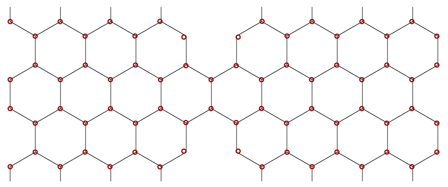
We now present some numerical results. Fig. 1 is the structure of our graphene junction system. The center region consists of two atoms, while the two leads are symmetrically arranged as strips (with periodic boundary conditions in the vertical direction). We obtained the force constants using the second generation Brenner potential. To compute the transient results, we need to perform convolution integrations in the time or frequency domain many times. It is handled by treating the convolutions as matrix multiplications. Then the expression of the derivatives, $\langle\langle Q^{n}\rangle\rangle=\partial^{n}\ln Z/\partial(i\xi)^{n}$, is calculated. Note that the $\xi$ dependence only enters through $\Sigma^{A}$. We also note that a power series in $\breve{G}\breve{\Sigma}^{A}$ terminates after $n$ terms for $\langle\langle Q^{n}\rangle\rangle$ for the product-state initial condition, but it is an infinite series for the steady-state case. The computational effort required for convergence is huge for the graphene junction. We also obtained the result for 1D chain which will be presented elsewhere.

Fig. 2 shows the first four cumulants. The first cumulant, which is also the first moment, is the total amount of energy entering the center from the left lead during time 0 to $t_{M}$. Its derivative gives the current. Such transient currents have been calculated [14] for the product initial states for 1D chains. The second cumulant gives the variance of $Q$. The higher order cumulants are small but not zero, thus the distribution of $Q$ is not gaussian. For large times, all the cumulants become linear in $t_{M}$, and are in agreement to the long-time prediction.

One striking feature of the results is that the product initial state and the steady-state initial state results behave qualitatively the same. The heat transferred, $\langle Q\rangle$, starts from 0 and goes down to negative values. This means whether we start from a decoupled system or a steady state, the effect of measurement is always to feed energy into the measured (left) lead, even if the temperature of the left lead is lower than that of the right lead. If the system were classical, the measurement cannot disturb the system. We should expect the current to be constant once the steady state is established. The nonlinear $t_{M}$ dependence observed here in $\langle Q\rangle$ is fundamentally quantum-mechanical in origin.

In summary, the generating function for phononic junction systems is obtained, which can be written compactly using Green’s function as $\ln Z=-(1/2){\rm Tr}\ln(1-G\Sigma^{A})$. A central quantity is the self-energy $\Sigma^{A}$ which is expressed in terms of the usual lead self-energy with shifted arguments. This is a very general result valid for steady-state initial states or product initial states in a two-time measurement. Numerical results for a graphene junction system are presented. An intriguing feature is that a measurement, even in the steady state, causes energy to flow into the leads. We hope that such robust features can be verified experimentally.

This work is supported in part by a URC research grant R-144-000-257-112 of National University of Singapore.

References

- [1] L. G. C. Rego and G. Kirczenow, Phys. Rev. Lett. 81, 232 (1998).
- [2] K. Schwab, E. A. Henriksen, J. M. Worlock, and M. L. Roukes, Nature 404, 974 (2000).
- [3] T. Yamamoto and K. Watanbe, Phys. Rev. Lett. 96, 255503 (2006).
- [4] J.-S. Wang, J. Wang, and J. T. Lü, Eur. Phys. J. B 62, 381 (2008).
- [5] L. S. Levitov and G. B. Lesovik, JETP Lett. 58, 230 (1993); L. S. Levitov, H.-W. Lee, and G. B. Lesovik, J. Math. Phys. 37, 4845 (1996).
- [6] W. Belzig and Y. V. Nazarov, Phys. Rev. Lett. 87, 197006 (2001); Y. V. Nazarov and M. Kindermann, Eur. Phys. J. B 35, 413 (2003); K. Schönhammer, Phys. Rev. B 75, 205329 (2007).
- [7] M. Esposito, U. Harbola, and S. Mukamel, Rev. Mod. Phys. 81, 1665 (2009).
- [8] C. Flindt, C. Fricke, F. Hohls, T. Novotný, K. Netočný, T. Brandes, and R. J. Haug, PNAS, 106, 10116 (2009).
- [9] K. Saito and A. Dhar, Phys. Rev. Lett. 99, 180601 (2007); Phys. Rev. E 83, 041121 (2011).
- [10] G. Gallavotti and E. G. D. Cohen. Phys. Rev. Lett. 74, 2694 (1995); C. Jarzynski, ibid. 78, 2690 (1997).
- [11] P. Talkner, P. S. Burada, and P. Hänggi, Phys. Rev. E 78, 011115 (2008).
- [12] R. P. Feynman and F. L. Vernon, Ann. Phys. 24, 118 (1963).
- [13] K. Saito and Y. Utsumi, Phys. Rev. B 78, 115429 (2008); D. Andrieux, P. Gaspard, T. Monnai, and S. Tasaki, New. J. Phys. 11, 043014 (2009).
- [14] E. C. Cuansing and J.-S. Wang, Phys. Rev. B 81, 052302 (2010); erratum 83, 019902(E) (2011).