Measuring gravito-magnetic effects by multi ring-laser gyroscope
Abstract
We propose an under-ground experiment to detect the general relativistic effects due to the curvature of space-time around the Earth (de Sitter effect) and to rotation of the planet (dragging of the inertial frames or Lense-Thirring effect). It is based on the comparison between the IERS value of the Earth rotation vector and corresponding measurements obtained by a tri-axial laser detector of rotation. The proposed detector consists of six large ring-lasers arranged along three orthogonal axes. In about two years of data taking, the sensitivity required for the measurement of the Lense-Thirring drag can be reached with square rings of side, assuming a shot noise limited sensitivity (). The multi-gyros system, composed of rings whose planes are perpendicular to one or the other of three orthogonal axes, can be built in several ways. Here, we consider cubic and octahedron structures. The symmetries of the proposed configurations provide mathematical relations that can be used to study the stability of the scale factors, the relative orientations or the ring-laser planes, very important to get rid of systematics in long-term measurements, which are required in order to determine the relativistic effects.
pacs
42.15.Dp, 42.30.Sy, 42.55.Lt, 91.10.NjI Introduction
The general theory of relativity is the most satisfactory description of gravitational phenomena. The theoretical breakthrough came with Einstein’s geometrical representation of gravity: as different test masses fall in the same way in a gravitational field, gravity must be a property of space and time rather than of the masses themselves.
Until now, almost all successful tests of general relativity (Shapiro time delay [5], light deflection by the sun [6], perihelion shift of the orbit of Mercury [7]) have been probing the gravitational field of the Sun, without considering its proper rotation. However, general relativity predicts that the stationary field of a rotating body is different from the static field produced by the same non-rotating mass. The difference is known as gravito-magnetism and consists of a drag of space-time due to the mass currents. The rotational frame-dragging effect is also known as the Lense-Thirring (LT) [8] effect.
A direct experimental evidence of the existence of the GM field has been obtained so far by Ciufolini [9] and by Francis Everitt and the GP-B group [3]. The Lense-Thirring effect, averaged over several orbits, has been recently verified by analysing the node orbital motion of two laser ranged freely falling satellites (LAGEOS-1 and LAGEOS-2) which orbit the Earth. In the measurement presented in Ref. [9] the two LAGEOS satellites were used to confirm the LT effect with an accuracy of the order of 10%. However, the launch of a third properly designed satellite LARES will give the opportunity to measure the LT effect with an accuracy of the order of 1% (citare).
The possibility to detect Lense-Thirring with ring lasers has been discussed in the past [53, 34] . Recently it has been already pointed out that a multi-gyros system is able to test locally the Lense-Thirring effect [10]: an array of six, side, square ring-lasers have enough sensitivity for this purpose. The rings must have different orientation in space. In the present paper we concentrate the attention on the symmetries of the rings arranged on the faces of a cube or along the edges of an octahedron, extracting the relevant relations important for the diagnostics of the system. At the end we summarize and sketch the proposed experiment. For completeness we must mention that an experiment of the type we are planning and preparing could also be made in principle using matter waves instead of light. This possibility has been proved experimentally for various types of particles such as electrons [12], neutrons [13], Cooper pairs [14], Calcium atoms [15], superfluid He3 [16] and superfluid He4 [17] . Cold atoms interferometry, in particular, yields very high sensitivity and it is suitable for space experiments because of the apparatus small size. However, atoms interferometry experiments in space do not provide an independent measurement of the Earth angular velocity, are affected by the mass distribution of the Earth, and test the average of the relativistic effect rather than the local one. Eventually, the comparison between in-space and on-ground measurements could be very valuable.
II Detection of Gravito-magnetic Effects
Gravito-magnetism (GM) is a general relativistic phenomenon related to the presence of mass currents in the reference frame of a given observer. In the case of celestial bodies, including the Earth, and excluding translational motion with respect to the center of the body, gravito-magnetic effects are due to the absolute rotation of the massive source with respect to distant stars. When the Einstein equations in vacuum are applied to this kind of symmetry and are linearised (weak field approximation) GM is accounted for by the analogue of a magnetic field of a rotating spherical charge. In practice at the lowest approximation level, a dipolar GM field is obtained, with the dimensions of an angular velocity. Its explicit form in a non-rotating reference frame centred on the source (in our case the Earth center), is (see e.g. [46])
| (1) |
where is the position of the laboratory with respect to the center of the Earth and is the angular momentum of the Earth, whose modulus is of course given by the product of the moment of inertia of the planet multiplied by its angular velocity.
The effect produced by a field like (1) on a massive test body moving with velocity looks like the one produced by a magnetic field on a moving charge: in fact, the geodesic equation in weak field approximation reads
| (2) |
where is the Newtonian gravitational field, so that the effect can be described in terms of a gravito-electromagnetic Lorentz force, where the Newtonian gravitational field plays the role of the gravito-electric field (GE).
Furthermore, the rotation of the source of the gravitational field affects a gyroscope orbiting around it, in such a way that it undergoes the so-called Lense-Thirring precession, or dragging of the inertial frames of which the gyroscope defines an axis[54, 46, 58]. This phenomenon shows up also when one considers a freely falling body with local zero angular momentum (ZAMO: Zero Angular Momentum Observer): it will be seen as rotating by a distant observer at rest with the fixed stars [18].
II.1 Mechanical gyroscopes
Gravito-magnetic effects can in principle be measured applying different methodologies. The one that has most often been considered is focused on the behaviour of a gyroscope, that can be either in free fall (on board an orbiting satellite) or attached to the rotating Earth. The axis of the gyroscope is affected in various ways by the presence of a gravitational field. As for GM, a little mechanical gyroscope is the analogous of a small dipolar magnet (a current loop), so that it behaves as magnetic dipoles do when immersed in an external magnetic field.
When studying the motion around the Earth of a gyroscope whose spin vector is , one is led to the formula [7, 46]:
| (3) |
In Appendix A we work out the explicit expression of in general relativity and, more in general, in metric theories of gravity, using the Parametrized Post-Newtonian (PPN) formalism[48]: we show that it is related to the gravito-magnetic components of the metric tensor and its expression is given by (see Eqs. (43)-(47)) , so that we can distinguish four contributions, namely the geodetic term , the Lense-Thirring term , the preferred frame term , the Thomas term . All terms in are called relativistic precessions, but properly speaking only the second is due to the intrinsic gravito-magnetic field of the Earth, namely it is , and manifests the Lense-Thirring drag.
Ciufolini [2] deduced the relativistic precession of the whole orbital momentum of two LAGEOS satellites whose plane of the orbit is dragged along by the rotating Earth. Again on Eq. (3) was based the GP-B experiment, whose core were four freely falling spherical gyroscopes carried by a satellite in polar orbit around the Earth [3]. While time goes on and the available data grow it is expected that the Lense-Thirring drag will emerge from the behaviour of the unique (so far) double pulsar system [4].
II.2 Using light as a probe
A different experimental approach consists in using light as a probe. In this case the main remark is that the propagation of light in the gravitational field of a rotating body is not symmetric. The coordinated time duration for a given space trajectory in the same sense as the rotation of the central source is different from the one obtained when moving in the opposite direction. This asymmetry would for instance be visible in the Shapiro time delay of electromagnetic signals passing by the Sun (or Jupiter) on opposite sides of the rotation axis of the star (or the planet) [20][21].
This property of the propagation of light is the one which we wish to exploit in our Earth-bound experiment using a set of ring lasers. In a terrestrial laboratory, light circulating inside a laser cavity in opposite directions is forced, using mirrors, to move along a closed path in space. What is closed from the view point of the laboratory is not so for a fixed-stars-bound observer, but the essential is that the two directions are not equivalent and that the two times required for light to come back to the active region are (slightly) different. As it happened already in the case of the mechanical gyroscopes, here too the difference in the two times of flight is made up of various contributions depending on the rotation of the axes of the local reference frame with respect to distant stars, on the fact that the local gravitational (Newtonian) potential is not null, and of course on the GM drag (which is our main interest). What matters, however, is that the final proper time difference (a scalar quantity) is invariant: it does not depend on the choice of the reference frame or of the coordinates.
Performing the calculation in linear approximation for an instrument with its normal contained in the local meridian plane (see the Appendix A details) we find
| (4) | |||||
where is the area encircled by the light beams, is the angle between the local radial direction and the normal to the plane of the instrument, measured in the meridian plane, and is the colatitude of the laboratory; is the rotation rate of the Earth as measured in the local reference frame (which includes the local gravitational time delay).
Eq. (4) can also be written in terms of the flux of an effective angular velocity through the cross section of the apparatus:
| (5) |
where is the area enclosed by the beams and oriented according to its normal vector . In particular, it is , and the term proportional to is the purely kinematic Sagnac term, due to the rotation of the Earth, while encodes the relativistic effects (see Appendix A)
For a ring laser in an Earth-bound laboratory, the geodetic and Lense-Thirring terms are both of order with respect to the Sagnac term, while the Thomas term is 3 orders of magnitude smaller. As for the preferred frame term, the best estimates [56, 57] show that this effect is about 2 orders of magnitude smaller than the geodetic and Lense-Thirring terms. Consequently, to leading order, the relativistic contribution to the rotation measured by the ring laser turns out to be , which we aimed at measuring in our experiment. In other words, the goal of our experiment will be the estimate of (see Fig. 1) which embodies the gravito-magnetic effects in a terrestrial laboratory.
In particular, the proposed experiment can also provide high precision tests of metric theories of gravity which are described in the framework of (PPN) formalism. In fact, from Eqs. (59-60), we see that, on setting for the rotating Earth , we obtain
| (6) | |||||
| (7) |
where and are PPN parameters (e.g. and in general relativity) which account for the effect of preferred reference frame and the amount of space curvature produced by a unit rest mass, respectively.
As shown in Sect. Discussions and Conclusions, from a high precision measurement of the vector in the meridian plane, we should be able to place new constraints on the PPN parameters and .
III Theory of the measurement: combining together the response of several rings
III.1 The response of a ring laser
A ring laser converts time differences into frequency differences. In fact, since the emission is continuous, the right handed beam adjusts itself to give a standing wave whose wavelength is an integer sub-multiple of the space length of the loop : . The same happens with the left handed beam, but being the total time different, also the wavelength of the corresponding standing wave will be different: . The two modes of the ring can have different , a situation usually called ’split mode’, but the higher accuracy of the measurement has been obtained so far with the two modes with equal . Considering the time of flight difference in terms of the wavelengths of the two standing waves we see that:
| (8) |
The ring laser equation [22] relates the frequency splitting of the two optical beams inside the ring interferometer with the experienced rotation rate of its mirrors
| (9) |
where is the perimeter and is the laser wavelength. The response of a ring laser to the rotation rate , in units of rad/sec, is simply a rescaling of the frequency splitting by the scale factor , i.e.
| (10) |
The scale factor plays a crucial role in the accuracy of the measurement of and to estimate the relativistic effects the ratio must be known and kept at accuracy level for months. The requirements to keep the apparatus in the optimal working conditions will be discussed in section IV.
Since the effective angular velocity as well as the gravito-magnetic one is of the order of , angles between vectors must be measured at the corresponding accuracy level. Unfortunately, the absolute measurement of in the fixed stars reference system with the accuracy of nano-radians can hardly be achieved. However, we can relax this requirement by using ring lasers oriented along directions (), where not all lie in the same plane. In fact, can be completely measured by means of its projections on at least 3 independent directions (e.g.defining a tri-dimensional Cartesian system) and the redundancies of the measurement can be used as a monitor and control of the stability of directions . We further assume that ring lasers have identical sensitivity and noise parameters. From an experimental point of view this can be easily satisfied by building the devices with scale factors that differ less than .
In order to simplify the sensitivity calculations of the system one can
consider multi-axial configurations endowed with symmetries. As all the ring
laser normals are equivalent in space, symmetric
configurations should be more efficient in the rejection of spurious effects
and in the control and monitoring of the relative orientation of the ring
lasers.
The natural choice is to take advantage of space symmetries of regular polyhedra, setting one ring for each plane parallel to their faces. If we do not consider the degeneration between opposite faces, we have M=3 in the case of the cube, 4 for tetrahedron and octahedron, 6 for dodecahedron, and 10 for icosahedron. There is a peculiar geometry with , obtained by arranging the rings along the edges of an octahedron, where the different rings can be nested together, sharing 2 by 2 the same mirrors. We will refer to it in the following by speaking of “octahedral configuration”.
The is the minimum number of rings necessary to reconstruct the rotational vector, but a redundancy is very appropriate to enhance statistic and to have control tests on the geometric accuracy.
In general, by simple arguments, one can demonstrate that, for regular polyhedra configuration
| (11) |
and that
| (12) |
As a consequence, one can study linear and quadratic combinations of ring
lasers responses which are invariant under permutations of the
ring laser labels , i.e. and .
For non-symmetric configurations we can generalize their definition as and , where and are suitable constants which
depend on .
The interest in such linear or quadratic forms relies on their behaviours in
the presence of noise fluctuations or variations of the geometry of the
configuration.
They also allow us to carry out analytical estimates of the overall
sensitivity of a tri-axial system of ring laser to relativistic effective rotation rates.
III.2 Requirements for the geometry of the configuration
The response of each ring laser can be conveniently written as
| (13) |
where account for systematic errors in the scale factors and orientations in space and represents the additive noise that affects the rotation measurement , that we assume averaged on the observation time . We assume as well that are Gaussian distributed random variables with zero mean and variance . Modulus and direction represent the deviations from regular polygon geometry in the plane and from polyhedra geometry in the space, due to scale factor fluctuations and infinitesimal rotations , respectively. In what follows the crucial assumption is that systematic errors (scale factors and relative alignment of ) are negligible with respect to statistical errors, i.e. or equivalently , while the dihedral angles can nearly approximate a regular polyhedron configuration.
Redundancy of responses, if rings are involved, can be used to control systematic errors projected along the direction of . In fact, the rigidity of the configuration imposes some linear kinematic constraints among different estimates of the laboratory rotation. In general, any linear combination of 3 responses gives an estimate of the local rotation and we can test the consistency among different estimates by means of the ordinary least square fit. A very simple linear constraint can be found for regular polyhedral configurations
| (14) |
and we will illustrate its statistical property as an example of the power of the method.
From the definition of immediately follows that it is Gaussian distributed with zero mean and standard deviation . In addition, possible misalignments or scale factor fluctuations are amplified by a factor of in the mean value of
| (15) | |||||
| (16) |
without affecting the corresponding variance . Thus can be used as a “null constraint” which is minimum when the configuration geometry is a regular polyhedron, and so the overall mean error parallel to can be monitored at accuracy level.
III.3 Estimate of the parallel component of the relativistic effective rotation vector
An estimate of for symmetric configurations readily follows from Eq. (12)
| (17) | |||||
| (18) |
Its mean value and standard deviation read (see App. B)
| (19) | |||||
| (20) |
In addition, one can demonstrate that is non-central distributed with degrees of freedom and non-centrality parameter . In order to estimate the relativistic effective rotation, we must subtract from the rotation rate estimated in the laboratory. To this end we calculate the difference that, in the limit of high SNR (), tends to be Gaussian distributed with mean
| (21) |
and standard deviation
| (22) |
where we have neglected terms of the order of . The of the parallel component of relativistic effective rotation is increased by a factor of with respect to the sensitivity of each ring laser.
The advantage of this approach is that we compare scalar quantities (moduli of rotation vectors) measured with respect to the local and distant stars reference systems. Its drawback is the very poor sensitivity to the perpendicular component of the relativistic effective rotation. In fact, , and the ratio between the second term (which is associated to the perpendicular component as ) and the first term is .
It is worth noticing that statistical fluctuations of (control of geometry by redundancy) and (measure of relativistic effects) are uncorrelated, and that they tend to be independent in the limit of high SNR.
III.4 Estimate of the components of the relativistic effective rotation vector
By arranging the response of ring lasers as M-tuples in a -dimension vector space , we can easily define projection operators that allows the estimate of local meridian plane and also the direction of in the physical space. Moreover, the norm of projected random vectors are described by remarkably simple statistics. According to the definition of the matrix product we have , where is a matrix whose elements are and . Thus, the random vectors can be projected on the linear subspaces and of dimensions 2 and , which represent respectively a plane in the physical space and its complementary space. The physical symmetry of the rotating Earth imposes that the relativistic effective rotation vectors and lie in the same plane, i.e. the meridian plane, and therefore the knowledge of the orientation of this plane is crucial if we want to measure not only the modulus but the whole vector. We recall that a plane is defined as the set of the points , where and range over all real numbers, and are given orthogonal unit vectors in the plane.
The parallelism of with the normal to the meridian plane can be tested under the hypothesis that the rotation signal is fully located in the subspace while the subspace contains only noise. The test can be easily performed over the norms of the two projections and , where we have introduced the symbol to indicate the L-2 norm in the M-dimensional Euclidean response space. The projection matrices and can be written explicitly as functions of the unit vectors and
| (23) | |||||
| (24) |
where is a matrix with columns and , and is the identity matrix. As shown in appendix B , the probability distribution of is non-central with 2 degrees of freedom and non-centrality parameter , while should be distributed with M-2 degrees of freedom.
The best estimate of and is then obtained by
| (25) |
where the is taken over the unit sphere. The direction of the Earth rotation axis can be estimated as a particular case of Eq. (10). In fact, the projectors and can be obtained by substituting the matrix for the matrix with columns . The difference lies in the dimension of the corresponding subspaces, i.e. and have dimension 1 and M-1 respectively. It is worth noticing that the maximum of Eq. (25) can be computed by an analytical formula both for the location of the meridian plane and the direction of the Earth rotation axis. In fact, if we introduce in the local reference frame the (local) spherical coordinate (, and ) (we use capital letters to avoid confusion with Sect. II) and parametrize the unit vectors and with these angles, for instance and , we have that the maximum of and is achieved for
| (26) |
where , , , are symmetric matrices which are functions of the alone.
In general, there are no analytical calculations for mean and variance of and one must run Monte Carlo simulations to get their estimates. However, in the limit of high SNR and tend to be Gaussian distributed, as well as fluctuations of and around their mean values. The same reasoning holds true also for the estimation of and .
The validity of the proposed experimental configuration has been checked by a numerical simulation over a period of 1 year of the six responses of the octahedral configuration oriented as in Fig. 23 of subsection V.3. In order to simplify the calculations we assume that the laboratory colatitude is and that the normal to the plane of a ring forms a angle with respect to the Earth axis, and another normal is orthogonal to the former and forms again a angle with the west-east direction. This configuration is close to a possible experimental arrangement at the Gran Sasso National Laboratories (LNGS) within few degrees. The directions of the unit vector in the local reference frame are
and the rotation signal for the 6 rings are equal within a factor .
We assume one mean sidereal day of integration and a noise standard deviation . The variance is extrapolated from present ”G” sensitivity at and scaling by a factor , due by the increase of the ring size and the power of the laser of a factor and , respectively. The relativistic rotation contributions and have been added to the Earth rotation vector , as estimated by IERS [28]. The component of relativistic effects parallel to is . Using Eq. (10) we calculated the responses of the 6 rings and then we injected the Gaussian noise. In Fig. 2 we show the histograms of accumulated for 90 and 366 sidereal days. The corresponding mean values of the parallel component of relativistic effects are and with standard deviations and , respectively. Thus a % accuracy can be achieved in 3 months by simply comparing the square modulus of rotation vectors. In order to give a full estimate of the vector , we have also explicitly calculated day by day the angles and for describing the orientation of the meridian plane and the direction of the Earth rotation vector. The results are summarized in Fig. 3 and 4, where we report the time evolution of these angles and in Fig. 5 where we show the corresponding annual polar motion.
By synchronizing the polar motion measured in the local reference system with the polar motion measured by IERS in the fixed star reference system, the two reference frames will coincide within the accuracy of the measurement of and , say 1 part of .
As a final remark, we point out that the full measurement of the vector allow us for the estimate of with a standard deviation of the same order of magnitude of the estimate of . This represent an increase of the relativistic rotation signal of %. However, the estimate of is crucial to separate the geodetic from Lense-Thirring contributions and/or to measure the PPN parameters and .
III.5 The Earth motion and feasibility of the experiment
Since our goal is the estimate of the Lense-Thirring effect at few % accuracy, the independent measurement of , which represents the rotation of the laboratory with respect to distant stars, must be determined to . Due to tidal forces and to the exchange of angular momentum between the solid Earth and geophysical fluids, the angular velocity of the Earth varies in time, both in direction and modulus. Changes in modulus correspond to a variation of the Length of the Day (LoD) of few milliseconds with respect to atomic clocks. The direction of the rotation axis of the Earth varies with respect to both the fixed stars and the Earth-fixed reference frames. Nowadays, the best Earth rotation monitoring is provided by the IERS 05C04 time series [28] which are routinely obtained using the geodetic space techniques VLBI (Very Long Baseline Interferometry), SLR (Satellite Laser Ranging), GPS ( Global Positioning System) and DORIS (Doppler Orbitography and Radiopositioning Integrated by Satellite).
In Figs. 6 and 7 we report the Length of the Day (LoD) and the pole position with the corresponding errors of the last six years. It is worth to noticing that the achieved precision is 0.001 ms in the LoD and in the pole position.

Further improvements are expected in the next few years and the overall errors in LoD and pole position should decrease of a factor 10 that is crucial for a 1% measurement of the relativistic rotation terms. However, the IERS 05C04 time series is already sufficient to get with accuracy.

For what concerns the differential rotation of the laboratory with respect to the rotation estimated by IERS, it is expected to be sufficiently small to contribute to only trough . However, is still largely unknown due to possible micro-rotations of the crust of the Earth. This is one of the causes limiting the performances of G in Wettzell: the Earth crust motion caused by atmospheric changes. It is assumed that an underground facility is less sensitive to this kind of noise sources. It is as well important to keep the experiment close to VLBI stations. The underground Gran Sasso Laboratories is placed half way between two relatively close VLBI stations, Medicina [29] and Matera [30] which can provide estimates of the crustal motion of the Adriatic plate [31]. A significant contribution to comes from the ”diurnal polar motion” (periodic motion of the Earth crust due to tides) and consists in periodic changes of amplitude . This effect has been already measured by large ring laser gyroscopes [35], and can be accurately modeled and then subtracted from ring lasers responses.
We conclude that by means of available geodesics and geophysics techniques, provided that the experiment is located in an area with very low relative angular motion (), a suitable tri-axial detector of rotation can in principle detect with precision.
IV The ’Real Apparatus’, the present sensitivity of G in Wettzell
Sensor properties
A closer look at equation 9 reveals that there are three basic effects one has to carefully account for. These are:
- •
scale factor stability ()
- •
orientation of the gyroscope with respect to the instantaneous axis of rotation of the Earth
- •
instantaneous rate of rotation of the Earth – Length of Day (LoD)
The scale factor for all practical purposes has to be held constant to much better than 1 part in . Otherwise the frame-dragging parameter cannot be determined unambiguously. For G, the base of the gyroscope has been manufactured from Zerodur, a glass ceramic with a thermal expansion coefficient of . Furthermore the instrument is located in a thermally insulated and sealed environment with typical temperature variations of less than 5 per day. However, because the underground laboratory is only at a depth of 5 m, there is still a peak to peak temperature variation of about 1 degree per year, accounting for the change of seasons. Changes in the atmospheric pressure also affect the dimensions of the ring laser structure by changing the compression of the Zerodur block and cannot be neglected. Hence G is kept in a pressure stabilized enclosure. A feedback system based on the determination of the current value of the optical frequency of the lasing mode of one sense of propagation allows for active control of the pressure inside the steel vessel such that an overall geometric scale factor stability of better than is routinely obtained. At the same time the design of the instrument is made as symmetric as possible. So changes in area and perimeter are compensated with a corresponding change in wavelength as long as no shear forces are present and the longitudinal mode index stays the same.
A typical eight day long measurement sequence of rotation rate data from the G ring laser is shown in Fig. 8. In order to demonstrate the obtained sensor sensitivity we have subtracted the mean Earth rotation rate from the gyroscope data.

The y-axis gives the measured variation of the rate of rotation, while the x-axis shows the time expressed in the form of the modified Julian date. Each data point was taken by integrating over 30 minutes of measurement data. There are several distinct signal contributions in the data, which come from known geophysical effects. The most prominent signal is caused by diurnal polar motion [25]. The polar motion data is superimposed by a tilt signal caused by the semi-diurnal and diurnal tides of the solid Earth, distorting the otherwise sinusoidal diurnal frequencies slightly. At the Geodetic Observatory in Wettzell the tilt effects of the solid Earth tides can be as large as 40 in amplitude. In Fig. 8 the diurnal signal is dominated by the polar motion [36]. Less evident in Fig. 8 are the effects from local tilt, which contains periodic signals of tidal origin as well as non-periodic signals. The latter are non-periodic and usually change slowly over the run of several days. High resolution tiltmeters inside the pressure stabilizing vessel of the G ring laser keep track of these local effects and the data is corrected for gravitational attraction (atmosphere, sun and moon)l [25]. Large non-periodic local tilts occur most prominently after abundant rainfall, indicating hydrological interactions with the rock and soil beneath the ring laser monument. Fig. 9 shows the east component of three tiltmeters installed i) on a gravimeter pillar at the surface, ii) in 6 depth, and iii) in 30 depth.

While the tilmeter in 30m depths clearly shows the periodic signal of the solid earth tides, the tilt record of the instruments near to the surface is dominated by large non-periodic signals hydrological, thermoelastic and barometric origin. Several investigations have shown that the site and the installation depths of tiltmeters has a major impact on environmental noise mainly coming from hydrology [41], [43], [44], [42] has shown that even in 100 depths effects caused by hydrological changes are detectable, but strongly reduced in comparison to a 50 deep installation. First investigations related to topographic and temperature induced effects were carried out by [39] and [40]. Detailed investigations using the finite-element method have shown that these effects can amount to more than 10 ([37], [38]), while the distance between the source and the location of observation can be several hundred meters. Additionally, recent work using the G ring laser data reveals that effects caused by wind friction at the Earth surface yields to high frequency rotations of large amplitudes.
The large seasonal temperature effect on the G ring laser as well as the substantial local tilt signals and the rather high ambient noise level of our near soil surface structures give reasonable hope of much better performances of a ring laser installation in a deep underground laboratory such as the Gran Sasso Laboratories.
For the detection of fundamental physics signals one has to remove all known perturbation signals of the Earth from the ring laser time-series. Furthermore we have applied 2 hours of averaging of the data in order to reduce the effect from short period perturbations. Fig. 10 shows an example.

In Fig. 11 we show the current sensitivity expressed in term of Allan deviation of the G, the expected sensitivity of each ring laser at Gran Sasso Laboratories and the relevant geophysical signal.

In order to reduce the local orientation uncertainties, which remain after local tilts measured with the high resolution tiltmeters have been removed, averaging as indicated above was applied to a series of 30 days of data collection, including the period shown in Fig. 8. It can be expected that a similar data set from the Gran Sasso laboratory would become substantially smoother, since most of the perturbations, caused by ambient atmosphere - topsoil interaction still contained in the data of Fig. 10 would no longer exist in the deep underground facility. Changing hydrologic conditions presumably causing small local rotation and temperature variations, atmospheric pressure and wind loading are among the sources for the systematic signatures in the residual data.
V Configuration of a tri-axial detector
From now on, we will restrict our analysis to perimeter rings, arranged in two configurations that are of some experimental interest, i.e. 6 ring lasers rigidly mounted on the faces of a cube, as shown in Fig. 12, and ring lasers oriented along the edges of an octahedron, see Fig. 13.


The cubic configuration requires mirrors forming independent rings and the extension of the GEOSENSOR design is straightforward (see subsection V.3 ); while the octahedral configuration require mirrors only to form orthogonal rings. By itself the configuration which uses a cube is redundant, each ring has a parallel companion, which can be used for the study of systematics. For the octahedron configuration the implementation of the GEOSENSOR design needs further development. Redundancy can be easily obtained constructing a second octahedron with planes parallel to the other one. The two structures should be built very close to each other, in order to keep as much as possible the whole apparatus compact; in this way rings are available, analogously to the cube configuration, see Fig. 14.

This configuration has the advantage that there are constraints in the relative angle between rings, since each mirror is in common between two rings, and three linear Fabry-Perot cavities are available using the three diagonals of the rings. Those linear cavities have the capability of monitoring the relative angles between different rings, and as well the length of each diagonal.
V.1 Ring-laser sensitivity
The rotation sensitivity , for noise fluctuations which are dominated by laser shot noise over an integration time T, reads
| (31) |
where is the quality factor of the optical cavity, is the laser frequency, is the Plank constant and is the power of the laser [27]. The limiting sensitivity can be conveniently calculated scaling the parameters of the Wettzell ”G” ring laser
| (32) | |||||
In order to obtain in few weeks a 10% accuracy level in the measurement of the relativistic effective rotation rates, we must achieve the sensitivity goal of (or equivalently a rotation noise level at a frequency of ). From Eq. (32) we have that a system of rings with , and can fulfill this requirement.
V.2 Expected performances of not optimally oriented rings
We assume that the ring lasers are identical in the sense described in Sect. III.5 and that the dihedral angles are measured better than one part in in order to estimate independently from the reference frame. Note that only the stability of dihedral angles can be monitored by means of the Earth signal itself only for short times (few days), while their measurements and controls must be performed independently in the laboratory. For instance, assuming that the scale factors are controlled to the accuracy, the responses of two parallel rings is statistically different from noise when their parallelism is modified.
From an experimental point of view, to arrange in the Cartesian planes several rings and keep the configuration stable over the integration time is a demanding task. However, we can relax such a demanding requirement by means of data analysis procedures that account for slightly non-orthogonal dihedral angles.
For instance, we can use the measured dihedral angles to estimate directly . In fact, we can substitute the quadratic combination of ring laser responses in Eq. (17) with the equivalent bilinear combination
| (33) |
where are the elements of the matrix . The statistics of is no longer non-central ; however, we can easily compute (see App. B for details) its mean
| (34) |
and variance
| (35) |
In the limit of high SNR, fluctuations of tend to be Gaussian distributed, and so we recover the results in Eq. (22) for the overall sensitivity of the system. If we start with dihedral angle close to (say 1 part in ), then sensitivity loss is very small since it is of the same order.
V.3 Guidelines of the Experimental Apparatus
The best performing ring, so far, is G which is a four mirrors ring. This is one of the reasons why the present scheme
uses a square ring geometry. In principle a triangular ring, with mirrors could be preferable since the three mirrors
are always inside a plane, and the losses will be minimized as well, reducing the number of mirrors. It could be advantageous in principle,
but a triangular ring is less sensitive. For instance, let us compare the performance of two rings inscribed in a circle
of radius ; for a regular polygon with different number of sides ,
the area is and the perimeter is
; it is straight forward to demonstrate
that the triangular ring has times the signal than the square one,
which is equivalent to say that the triangular ring needs times more
time to reach the same level of accuracy as the square one.
The ring-laser response is proportional to the Scale Factor ”S”. For a perfect
square ring this proportionality factor is equivalent to the number of wavelength
inside the ring: when the length of the ring changes, because of a change in the temperature,
the laser changes its wavelength in order to keep constant. This is true as long as the
perimeter change is below a wavelength, in our case, and in this conditions the
gain factor of the instrument guarantees a very high accuracy of the measurement.
For example: if the laboratory has degree temperature excursion, the ring perimeter is ,
in order to guarantee the operation of the ring-laser with a fixed number of wavelengths , it is
necessary to realize the whole apparatus using materials with temperature expansion coefficient of the order of . This is the concept used for G in Wettzell: a structure realised with material as Zerodur, with a design which can be defined monolithic, i.e. relative motions of the mirrors are not allowed. G has a very high stability, but is rather expensive, and not very flexible with regards to changing the mirrors and align the laser cavity. Moreover the extension of this design to a large array of rings seems rather difficult. Later on, a more flexible and less expensive design has been realized, called GEOSENSOR, which so far has been employed especially for smaller size rings. This design allows a very good relative alignment of the mirrors, it is relatively easy to change mirrors and tools to move each mirrors along different degrees of freedom have been implemented. So far this kind of instruments have been done in steel.
Fig. 15 shows a drawing of G-Pisa, our prototype.

The optical cavity vacuum chamber has a stainless steel modular structure: 4 towers, located at the corners of the square and containing the mirrors holders inside, are connected by pipes, in order to form a ring vacuum chamber with a total volume of about m3. The mirrors are rigidly fixed to the tower. The cavity alignment can be adjusted by moving the towers with respect to the slab through a lever system that allows degrees of freedom of movements. No window delimits the active region and the vacuum chamber is entirely filled with a mixture of He and a isotopic mixture of 20Ne and 22Ne. The total pressure of the gas mixture is set to 560 Pa with a partial pressure of Neon of . The active region is a plasma produced in a capillary pyrex tube inserted at the middle of one of the ring sides by a radio frequency capacitively coupled discharge. In a non monolithic device, temperature changes could interrupt the continuous operation, and the perimeter is actively controlled by acting on the mirrors and using as reference a stabilized laser; very highly stabilised lasers are commercially available, for instance wavelength stabilization at the level of using iodine line can be obtained. G-Pisa is kept in continuous laser operation trough a perimeter stabilization servo system which acts along the diagonal direction, for two opposite placed mirrors, through piezoelectric actuators [52] .
The GEOSENSOR design has other advantages as well: the mirrors are under vacuum and are not affected by the outside pressure changes, they can be very easily aligned and the cost is pretty much reduced compared with the monolithic design. The experience of G-Pisa has shown so far that it can work with different orientations. In fact G-Pisa has worked both horizontally and vertically oriented. It is in steel, inside the thermally stabilized room in the central area of Virgo, in order to improve thermal stability, it has been mounted on top of a granite table (thermal expansion coefficient about ).
To find the guidelines of the mechanical project, we have used a simple program which consists in considering the ring as four points (the light spot on the mirrors) which can be moved from the ideal position, both inside the plane or outside the plane. The model takes into account thermal expansion and the perimeter is kept constant by acting diagonally on pairs of mirrors; the use of mirrors or mirrors for the feedback correction have been investigated; the thermal excursion is considered of degree. The scale factor in presence of misalignments is compared with ( scale factor at the optimal configuration); this comparison is expressed as , which gives the accuracy limit induced by misalignments. The required level of accuracy of part of is .
Fig. 16 shows for a rectangular ring, with sides and , in function of a misalignment of one of the four mirrors.
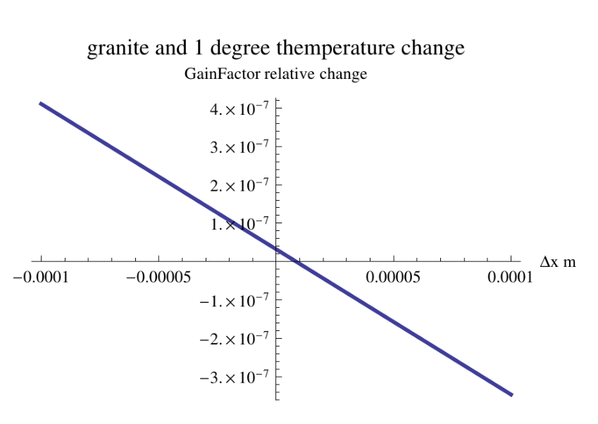
Fig. 16 clearly shows that the Gain Factor changes a lot with small change of mirrors positions. The situation strongly improves by considering a perfect square ring. In fact, for a closed figure with a fixed number of sides, the area over perimeter ratio has a maximum when the polygon is regular one, as for example a ’perfect’ square ring. Fig. 17 and 18 show with construction precision and two possible choices of the thermal expansion coefficient.
For instance, let us assume that each mirror position is in the ideal position within a quantity which depends on the precision of the construction. Fig. 19 shows when out of the mirrors are positioned with an error, points have been evaluated pseudo-randomly distributed between along each coordinate.
In summary, if the thermal excursion is , the position of the mirrors is an ideal square within , the support has a thermal expansion coefficient below , remains in the range necessary for the needed accuracy using four or two mirrors active control of the perimeter.
Misalignments which bring the light spots outside the plane of the ring do not have appreciable effect on the gain factor, but they change the orientation of area vector ; in this case the effect for depends on the relative angle between the ring and the Earth rotational axis. Figs. 20 and 21 shows how the accuracy changes for two different ring orientations: parallel to the axis of the Earth and at degrees respectively. The first is almost insensitive, while the other is sensitive to nano-metric misalignments.
Fig. 22 shows for a vertical misalignment of one of the rings in function of the angle with respect to the Earth rotational axis.
In summary: The Gain Factor of each ring can be kept constant at the level of part in , if the positions of the mirrors are constructed and kept within error close to the ideal square ring; the relative position between mirrors can be rigidly constrained with granite, super-invar or similar low thermal expansion coefficient spacers, it is preferable to use all the four mirrors for the perimeter active stabilization, but two mirrors control could be acceptable as well if the structure has thermal coefficient better than granite. It is necessary to constantly monitor the relative angle between rings with precision (only the relative alignment matters). This can be accomplished looking at the modal structure of the FP cavities formed along the diagonals.
Moreover the orientation of each ring with respect the Earth rotation axis should be such to avoid alignment too sensitive to the relative angle (relative angle with the Earth rotation axis below ).
Using the Earth angular velocity rotation, which is perfectly stable for few days, the whole apparatus can be calibrated at the beginning; the relative angle, or the area of each ring could be not perfectly planar or exactly , but it is important to monitor the geometry of the structure during the whole measurement time (years). The mirror holders plays an important role, it can be advantageous to build them in Zerodur or similar material, in order to avoid displacements out of the plane. The mirrors holder should be designed in order to provide the tools to align the cavities; in principle each mirrors should have degrees of freedom: translations and two tilts, the rotation around the axis orthogonal to the mirror itself does not play a role; but since the mirrors are spherical only three motions are fundamental: we may have one translation along the diagonal and two mirrors tilts or three translations.
Let us consider now an octahedral geometry, containing the three rings.
Fig. 22 shows that the relative angle between the different rings must be monitored at the level of nrad, and that it should be avoided to put one of the rings with an angle larger than with respect the Earth rotation axis. We have done the exercise to fit the octahedron, with rings of perimeter, inside the node B of LNGS, considering that this node is tall, and imposing the constrains discussed in Fig. 22. The exercise is done with the octahedron since it needs more space. Considering that the latitude of LNGS is two configurations are given: to have the octahedron straight up ( tall) or laying on one side, one ring is respectively horizontally or vertically oriented and the other two symmetrically positioned with respect to the meridian plane. Let us consider the maximum size : , the diagonal of the octahedron, plus necessary to hold mirrors and optics in general necessary for the read out. This octahedron can be contained inside each of the big halls of LNGS, in both orientation, but inside node B, which is the most isolated room of LNGS, see Figs. 23 and 25, the only possibility is the shorter configuration, with the longer side parallel to the floor.

So, the octahedron, with rings of perimeter, can be contained inside node B, where the ceiling is tall, while for node C the structure should be scaled, probably no more than perimeter can be contained inside node C, since the ceiling there is tall. Fig. 24 shows the octahedron inside node B.


VI Diagnostics of dihedral angles and scale factors
To reduce the influence of systematics in long–term measurements, the control of the geometrical stability of ring laser system is of paramount importance. In particular, it is crucial to monitor the deviations from planarity of each ring laser and their mutual orientations.
A square ring consists of four spherical mirrors with the same curvature radius , placed at the corners. Square geometry guarantees that opposite mirrors are parallel so that they form two extra linear Fabry–Peròt cavities (see Fig. 26). As a consequence, each square ring is made of three optical resonators: the ring itself and two linear ones oriented along the diagonals. These latter can be used to monitor the geometrical stability of the whole ring system. Deviations from a square geometry result in tilting and/or displacements of the diagonal vectors, which in turn change the cavity eigenmodes.
A linear symmetric FP cavity with spherical mirrors in ( being the square ring arm) and centers on the z-axis, supports the Gaussian modes
| (36) |
where and are the complex curvature of the Gaussian beam and the confocal parameter, respectively; here the curvature radius and the spot-size read
The eigenmodes form a complete set which can be used for representing a generic field confined between the two generally misaligned mirrors of the cavity
where
and is the beam illuminating the input mirror . If we suppose the mirror tilted by and and displaced by and with respect to cavity axis , we have
As an example, the relative intensities for the first modes and are reported in Tab. 1.
It is clear that the cavity axes misalignment can be detected by looking at the intensity pattern of the beam transmitted though the output mirror . A modal decomposition of such a pattern gives a suitable set of coefficients which can be used for estimating the position and angular misalignment of the cavity with respect to the reference beam .
Supposing that at the begining () the cavity external laser is perfectly aligned to a symmetric cavity (if the two mirror show equal transmittivity then the cavity transmission is ) so that all the incoming power is coupled to the TEM00 mode. The measurement procedure we have devised is a tunable laser, showing a linewidth narrower than the cavity linewidth, tuned over a cavity FSR in a time interval so that each mode is spanned in a time , where is the cavity finesse. The number of photons in the mode are given by (we are now assuming a rectangular line shape instead of a Lorentzian profile)
This number of photons must be higher than the noise equivalent number of photons hitting the detector in the same time interval. The noise equivalent power in , is connected to the equivalent number of photons by
where and are the quantum efficiency and the detection bandwidth, respectively.
To overcome the photon noise, we have to satisfy the inequality
In particular, looking at coefficient we have
further, by assuming we obtain
For typical silicon detectors , , , so that
For a tilt sensitivity of the power required at the input is

VII More about the importance of this measurement
VII.1 Post Newtonian Parameters
The proposed experimental apparatus is well suited for performing optical test of metric theory of gravitation. We start from the statement that the vector should be entirely contained in the meridian plane if the preferred frames effect, determined by (see Eq. (A9)), can be neglected. Indeed the currently available best estimates [48] suggest that this effect is about 2 orders of magnitude smaller than the geodetic and Lense-Thirring contributions. As a consequence, we expect that the measured components of outside the meridian plane should be compatible with noise. In this case, our results could be used to obtain new constraints, independent from the available ones, on the preferred frames parameters. In addition, we can write the PPN parameters and as a function of the and components of
| (37) |
where and is the very precisely measured constant ; here we have used , and . Assuming one year of data taking with the same ring laser parameters used for the simulations in Sect. IIID we have that the standard deviation of and is , and therefore upper limits of some interest can be put on and at the Gran Sasso colatitude .
VII.2 Interdisciplinary: Geodesy and Geophysics
Earth rotation rate and the orientation of the rotational axis of the Earth in space are the linking quantities between the terrestrial (ITRF) and the celestial (ICRF) reference frames. Currently a set of quasars, forming an external set of markers, provide the only way of determining the rotational velocity and the variations of the orientation of the rotational axis of the Earth with sufficient accuracy. As already mentioned, for the measurement of length of day (LOD) and for the pole position are routinely achieved by a network of VLBI radio telescopes as one of the services (IERS) of the International Association of Geodesy (IAG). The operation of such a network requires expensive equipment and a lot of maintenance effort. Huge amounts of data are recorded in each measurement session, which require physical transport over large distances for the correlation in the analysis centers. Data latency and the fact that there is no continuous measurement coverage are suggesting the investigation of alternative methods for the precise estimation of Earth rotation. Furthermore it is desirable to develop an independent measurement technique, in order to identify intra-technique biases if they exist. Ring lasers are possible candidates for such an alternative measurement technique. They measure the earth rotation locally and within much shorter time intervals. Such gyros are widely used in aircraft navigation and can measure rotations absolute, i.e. independent of an external reference frame. Therefore also local contributions to earth rotation are contained in the measurements. The effects of earth tides, strain, crust deformation, seismic events, polar motion are contained in the ring laser measurements due to their contribution to earth rotation or due to variations in the orientation of the respective ring laser. However, the demands on such instruments are extremely high and cannot be met by existing commercial devices. They can be summarized as:
- •
sensitivity to rotation at about 1 hour of integration
- •
sensor stability of 1 part in over several month to years (Chandler Wobble)
- •
resolution in sensor orientation . This corresponds to polar motion of around at the pole.
This means that a reasonable improvement in sensor sensitivity and stability is still required in order to make ring lasers viable tools to be applied to space geodesy. The design of the G ring laser is one way of approaching these demands and it not too far away from reaching this goal [45]. Operating several such ring laser gyroscopes in geophysical independent regions simultaneously offers a unique possibility to distinguish global from local (monumentation related) signal contributions through their independent data streams.
Discussions and Conclusions
The feasibility of the experiment for the measurement of relativistic effective rotation rates appears to rest only on a tri-axial dynamical sensor of local rotation of enough sensitivity. Despite the fact that large ring lasers as G are very stable platforms and with the provision of tight feedback systems to stabilize the scale factor (cold cavity, as well as the active cavity), currently ring laser gyroscopes are not able to determine the DC part of the Earth rotation rate with a sensitivity compatible with the requirements for detection of the Lense-Thirring effect. While the contribution of the varying Earth rotation itself presumably can be removed with sufficient accuracy from the C04 series of VLBI measurements, there remains the problem of determining the actual null-shift offsets from the laser functions in the ring laser gyroscope. Since the gravito-magnetic effect is small and constant, a good discrimination against laser biases, such as for example ‘Fresnel drag’ inside the laser cavity must be achieved. Therefore it will be advantageous to add one or several ring laser cavities in addition to the triad structure for sufficient redundancy. We also intend to operate at least the G ring laser structure in parallel to the here proposed structure in order to discriminate local perturbation signals from regional and global ones. A second large ring laser located at the Cashmere facility in Christchurch, New Zealand, will be used in the data analysis process, provided it can be run with sufficient resolution and stability.
Appendix A Ring Laser Measurements in the Laboratory Frame
In this Appendix we evaluate the response to the gravitational field of a ring laser in an Earth bound laboratory and, to know the space-time metric in the laboratory frame we shall use the construction of the “proper reference frame” as described in Ref. [46, 7].
As we discussed in Section III, a ring laser converts a time difference into a frequency difference (see e.g. Eq. (8)). It is possible to show that (see e.g. [55]) in a stationary metric in the form11 1 Greek and Latin indices denote space-time and spatial components, respectively; letters in boldface indicate spatial vectors, while letters in italic indicate four-vectors and four-tensors; summation and differentiation conventions are assumed. In this Appendix, if not otherwise stated, we use units such that . an observer at rest at measures the proper-time difference between the right handed beam propagation time () and the left handed one ():
| (38) |
where is the spatial trajectory of the beams, whose tangent vector is , and we set
In order to evaluate the proper-time difference (38), we need to know the space-time metric in our laboratory, that is to say the gravitational field nearby the world-line of the observer which performs measurements with the ring laser. To this end, we consider an observer in arbitrary motion in a given background space-time, and write the corresponding local metric in a neighborhood of its world-line (see e.g. [7])
| (39) | |||||
| (40) | |||||
| (41) |
It is worth pointing out that the Eqs. (39)-(41) hold only near the world-line of the observer, where quadratic displacements terms are negligible. Here we suppose that the observer carries an orthonormal tetrad (parentheses refer to tetrad indices) , whose four-vector coincides with his four-velocity , while the four-vectors define the basis of the spatial vectors in the tangent space along its world-line. By construction we have , where is the Minkowski tensor. The metric components (39)-(41) are expressed in coordinates that are associated to the given tetrad, namely the space coordinates and the observer’s proper time . In the above equations, is the spatial projection of the observer’s four-acceleration, while the tensor is related to the parallel transport of the basis four-vectors along the observer’s world-line: . In particular, if were zero, the tetrad would be Fermi-Walker transported. Let us remark that the metric (39)-(41) is Minkowskian along the observer’s world-line (); it is everywhere flat iff , i.e. the observer is in geodesic motion and the tetrad is non rotating (i.e. it does not rotate with respect to an inertial-guidance gyroscope). In the latter case, the first corrections to the flat space-time metric are [7].
In order to explicitly write the local metric, which through its gravito-magnetic () and gravito-electric () components enables us to evaluate the proper-time difference (38), we must choose a suitable tetrad by taking into account the motion of the Earth-bound laboratory in the background space-time metric. To this end, we consider the following PPN background metric which describes the gravitational field of the rotating Earth (see e.g. [48]):
where is the Newtonian potential, is the angular momentum of the Earth, is the velocity of the reference frame in which the Earth is at rest with respect to mean rest-frame of the Universe; and are post-Newtonian parameters that measure, respectively, the effect of spatial curvature and the effect of preferred frames. The background metric () is referred to an Earth Fixed Inertial (ECI) frame, where Cartesian geocentric coordinates are used, such that is the position vector and . Then, we choose a laboratory tetrad which is related to the background coordinate basis of () by a pure Lorentz boost, together with a re-normalization of the basis vectors: in other words the local laboratory axes have the same orientations as those in the background ECI frame, and they could be physically realized by three orthonormal telescopes, always pointing toward the same distant stars.
In this case, one can show that the gravito-magnetic contribution in the local metric reads [7, 46, 49, 50] , where the total relativistic contribution is the sum of four terms, with the dimensions of angular rotation rates
| (43) |
defined by
| (44) | |||||
| (45) | |||||
| (46) | |||||
| (47) |
The vector represents the precession rate that an inertial-guidance gyroscope, co-moving with the laboratory, would have with respect to the ideal laboratory spatial axes (see e.g. [7, 46]) which are always oriented as those of the ECI frame; if the spin vector of the gyroscope is , its precession is hence defined by
| (48) |
Differently speaking, we may say that the local spatial basis vectors are not Fermi-Walker transported along the laboratory world-line. In particular the total precession rate is made of four contributions: i) the geodetic or de Sitter precession is due to the motion of the laboratory in the curved space-time around the Earth; ii) the Lense-Thirring precession is due to the angular momentum of the Earth; iii) is due to the preferred frames effect; and iv) the Thomas precession is related to the angular defect due to the Lorentz boost.
It is worth noticing that for a laboratory bounded to the Earth
| (49) |
and the acceleration can not be eliminated. However, for a geodetic motion (e.g. a free fall satellite) and by substituting in Eqs. (44) and (47), we obtain
| (50) |
and
| (51) |
Eq. (50) gives the geodetic precession for a free fall gyroscope, while Thomas precession (51) is zero.
All terms in (44)-(47) must be evaluated along the laboratory world-line (hence, they are constant in the local frame), whose position and velocity in the background frame are and , respectively. However, if we consider an actual laboratory fixed on the Earth surface, the spatial axes of the corresponding tetrad rotate with respect to the coordinate basis of the metric (), and we must take into account in the gravito-magnetic term (40) the contribution of the additional rotation vector , which corresponds to the Earth rotation rate, as measured in the local frame22 2 For an Earth-bounded laboratory, it is where is the terrestrial radius, is the colatitude angle of the laboratory and is the terrestrial rotation rate, as measured in an asymptotically flat inertial frame..
As a consequence, it is possible to show that, up to linear displacements from the world-line, the relevant local gravito-magnetic potential turns out to be
| (52) |
where , while the gravito-electric one remains the same.
Now, we are able to evaluate the proper-time difference
| (53) |
Without loss of generality, we suppose that the observer is at rest in the origin of the coordinates, so that, according to (39), . As a consequence, we have
| (54) |
Now, on taking into account the expression of acceleration of the laboratory frame (49) and evaluating the magnitude of the various terms, the leading contribution to (54) con be written, applying Stokes theorem
| (55) |
where is the area enclosed by the beams and oriented according to its normal vector . On evaluating the curl, taking into account that is constant, we eventually obtain
| (56) |
On substituting in (56), we see that the proper-time delay can be written in the form
| (57) |
where is the purely kinematic Sagnac term, due to the rotation of the Earth, while is the gravitational correction due to the contributions (44)-(47).
According to Section III.1, from Eq. (56), it is then possible to write the ring laser equation in the form
| (58) |
To further clarify Eqs. (44)-(47) it is useful to use an orthonormal spherical basis in the ECI frame, such that the plane coincides with the equatorial plane. As a consequence, the position vector of the laboratory with respect to the center of the Earth is and the kinematic constraint holds, i.e. .
Thus, the components of in physical units read
| (59) | |||||
| (60) | |||||
| (61) | |||||
| (62) |
Moreover, we assume the general relativistic values of the PPN parameters, , and use for the Newtonian potential of the Earth its monopole approximation, i.e. . Thus, the components (59)-(60) read
| (63) | |||||
| (64) | |||||
| (65) | |||||
| (66) |
and, to leading order, the total rotation rate which enters the Eq. (57) is
If we denote by the angle between the radial direction and the normal vector , on setting in (57), and using (), we may express the proper-time delay in the form
| (68) |
where we have written , in term of the , the moment of inertia of the Earth.
Appendix B Probability Distribution of Quadratic Forms
The statistics of quadratic forms of Gaussian random vectors are well known in the literature. In particular, if is a multivariate Gaussian random vector with mean and covariance matrix , the mean and the variance of a quadratic form are given by
| (69) | |||||
where is a square symmetric matrix, and are the transpose and trace operators, respectively. The statistics of in general is not known, unless is an idempotent matrix [51]. In the case were represents the response of ring lasers in a regular polyhedral configuration , with no common noise source and the same sensitivity , where is the identity matrix, the above formulas greatly simplifies
| (70) | |||||
| (71) |
where is the signal energy. In this case also the statistics of readily follows. In fact, starting from its definition we have
| (72) |
where is the Gaussian probability density of one sample of the random vector . We can use the integral representation of the Dirac’s -function
| (73) |
and write
By re-arranging the exponent, the last integral can be recast as a M-dimensional Gaussian integral and calculated explicitly
| (74) |
where in the last expression one recognizes the moment generating functions of a non-central distributions with degrees of freedom and non-centrality parameter . The probability density function of can be found using the tables of Fourier Transform pairs
where are the modified Bessel functions of order .
Appendix C Probability Distribution of Projectors
The norm of complementary projection operators and acting on Gaussian random vectors are described by remarkably simple statistics. In fact, starting from the definition of and we have that the joint probability density reads
| (75) |
where is the probability density of one sample of the random vector . The two Dirac -functions can be written using their Fourier transforms,
| (76) |
where the integrals in and are performed along the imaginary axis (i.e. and are purely imaginary complex numbers). Now assume the noise is Gaussian distributed, uncorrelated between different detectors and with identical variance in every detector, namely
| (77) |
where is the rotation signal in vectorial form. Then,
| (78) | |||||
where . Writing as and switching the integration variable to yields
| (79) | |||||
The integration in can be done by noting that it is a standard -dimensional Gaussian integral with the linear term, and in general, for any symmetric matrix and -vector ,
| (80) |
In our case,
| (81) |
Now we exploit the properties of and . Using their complementarity, we can write
| (82) |
and from the fact that they are orthogonal and idempotent we also have
| (83) |
hence
| (84) |
Furthermore, as and are projection matrices, their eigenvalues are with multiplicities respectively for and for . Then, writing in diagonal form is trivial and leads to
| (85) |
determinants being independent from the basis. By using 84 and 85 in 80 one can see that the Gaussian integral splits into the product of factors involving either or . By further substituting in 79, the remaining integrals separate and the probability density remarkably factorizes as
| (86) |
with
and , . The transformed functions is the moment generating functions of two non-central distributions, with 2 and degrees of freedom respectively, and whose non-centrality parameters are and respectively. Thus,
where is the modified Bessel function of the first kind. Some interesting conclusions can be drawn about the virtual channels and , which make them interesting for the identification of meridian plane and the estimate of .
- 1.
is distributed as a non-central with 2 degrees of freedom and non-centrality parameter equal to , i.e. the magnitude of the signal projection in the P subspace.
- 2.
is distributed as a non-central with degrees of freedom and non-centrality parameter equal to , i.e. the magnitude of the signal projection in the subspace.
- 3.
and are statistically independent processes.
- 4.
In the limit of high SNR, and are Gaussian distributed with means , and variances , , respectively.
References
- [1] , Will, C.M. Theory and Experiment in Gravitational Physics, Cambridge University Press (1993)
- [2] Ciufolini, I. The 1995-99 measurements of the Lense-Thirring effect using laser-ranged satellites, Class. Quantum Grav. 17 2369 (2000)
- [3] Everitt, C.W.F. et al.. Gravity Probe B: Final Results of a Space Experiment to Test General Relativity, Phys. Rev. Lett., in press (2011).
- [4] Bourgay M., et al., An increased estimate of the merger rate of double neutron stars from observations of a highly relativistic system, Nature 426, 531-533 (2003)
- [5] I.I. Shapiro et al., Phys.Rev. Lett., 26, (1971) 1132
- [6] Straumann, N., General Relativity and Relativistic Astrophysics, Springer-Verlag, Berlin (1991)
- [7] Misner, C.W., Thorne, K.S., Wheeler, J.A., Gravitation, Freeman, S. Francisco (1973)
- [8] H. Thirring, Phys. Z., 19, (1918) 204
- [9] I. Ciufolini, E. Pavlis, Nature 431, 958 (2004); I. Ciufolini et al, 71-104, Space Sci Rev (2009) 148.
- [10] Di Virgilio, A. et al., A laser gyroscope system to detect the Gravito-Magnetic effect on Earth, Int. J. Mod. Phys. D, 19 2331-2343 (2010)
- [11] Triangular ring laser, perimeter, Univ. of Christchurch, NZ
- [12] Hasselbach F and Nicklaus M, Sagnac experiment with electrons: Observation of the rotational phase shift of electron waves in vacuum, Phys. Rev. A, 48 143 (1993)
- [13] Werner S A, Staudenmann J L and Colella R, Effect of Earth’s Rotation on the Quantum Mechanical Phase of the Neutron, Phys. Rev. Lett., 42 1103 (1979)
- [14] Zimmermann J E and Mercereau J E, Compton Wavelength of Superconducting Electrons, Phys. Rev. Lett., 14 887 (1965)
- [15] Riehle F, Kirsters Th, Witte A, Helmcke J and BordeĆh J, Optical Ramsey spectroscopy in a rotating frame: Sagnac effect in a matter-wave interferometer, Phys. Rev. Lett., 67 177 (1991)
- [16] R.W. Simmonds et al Nature 412 (2001) pag 55
- [17] E. Hoskinsons et al Phys. Rev. B74 (2006) 100509(R)
- [18] Raine, D. and Thomas, E., Black Holes - An Introduction, World Scientific, Singapore (2009)
- [19] C.W.F. Everitt et al, 53-69, Space Sci Rev (2009) 148.
- [20] A. Tartaglia, Clas. Q. Grav., 17, (2000) 2381-2384.
- [21] A. Tartaglia, A. Nagar, M.L. Ruggiero, Phys. Rev. D, 71, (2005).
- [22] G.E. Stedman, Ring-laser tests of fundamental physics and geophysics, Rep. Prog. Phys. 60, 615–688 (1997).
- [23] K.U. Schreiber, T. Klügel, A. Velikoseltsev, W. Schlüter, G.E. Stedman and J-P. R. Wells; The large ring laser G for continuous Earth rotation monitoring; Pure and Applied Geophysics, 166, No 8-9, 1485-1498, (2009).
- [24] K. U. Schreiber, G. E. Stedman and T. Klügel; Earth tide and tilt detection by a ring laser gyroscope, J. Geophys. Res. 108 (B)2, (2003)
- [25] K. U. Schreiber, A. Velikoseltsev,M. Rothacher, T. Klügel, G. E. Stedman, D. L. Wiltshire; Direct measurement of diurnal polar motion by ring laser gyroscopes J. Geophys. Res. Vol. 109, No. B6, B06405, (2004)
- [26] B. Pritsch, K.U. Schreiber, A. Velikoseltsev and J-P. R. Wells; Scale factor corrections in large ring lasers; Applied Physics Letters, 91, No. 6, 061115, (2007),
- [27] K.U. Schreiber, J-P. R. Wells and G.E. Stedman; Noise processes in large ring lasers; General Relativity and Gravitation, 40, No. 5, 935-943, (2008)
- [28]
Time series of the daily estimate of Earth rotation vector
can be downloaded from
http://data.iers.org/products/176/11165/orig/eopc04.62-now - [29]
See e.g.
http://www.med.ira.inaf.it/index_EN.htm - [30]
See e.g.
http://www.asi.it/en/flash_en/observing/space_geodesy_center - [31] E. Mantovani, D. Albarello, C. Tarnburelli, M. Viti, Annals of Geophysics 38, 67 (1995); R. Haas, E. Gueguen, H. Scherneck, A. Nothnagel, and J. Campbell, Earth Planets Space, 52, 759-764, (2000).
- [32] K. U. Schreiber, et al. Journal of Geophysical Research, 109, B06405 (2004).
- [33] G.E. Stedman, R.B. Hurst and K.U. Schreiber; On the potential of large ring lasers, Optics Communications, 279, No. 1, 124-129, (2007).
- [34] Scully, M.O., Zubairy, M.S., Haugan, M.P., Proposed optical test of metric gravitation theories, Phys. Rev. A 24, 2009 (1981).
- [35] Schreiber, K.U. et al., J. Geophys. Res. 109, B06405 (2004).
- [36] Brzezinski, A., Contribution to the theory of polar motion for an elastic earth with liquid core, Manuscr. Geod., 11, 226-241 (1986).
- [37] Gebauer, A.; Kroner, C.; Jahr, T., The influence of topographic and lithologic features on horizontal deformations, Geophys. J. Int., 177, 586-602 (2009).
- [38] Gebauer, A.; Steffen, H.; Kroner, C.; Jahr, T., Finite element modelling of atmosphere loading effects on strain, tilt and displacement at multi-sensor stations, Geophys. J. Int., 181 (3), (2010).
- [39] Harrison, J.C., Cavity and topographic effects in tilt and strain measurements, JGR, 81/2, 319-328 (1976).
- [40] Harrison, J.C., Herbst, K., Thermoelastic strains and tilts revisited. Geophysical Research Letters, 4/11 (1976).
- [41] Jentzsch G.,Liebing M.,Weise A., Deep Boreholes for High Resolution Tilt Recording. Bulletin Inf. Marees Terrestres, 115, 8498-8506 (1993).
- [42] Jahr, T., G. Jentzsch, A. Weise, Natural and man-made induced hydrological signals, detected by high resolution tilt observations at the Geodynamic Observatory Moxa/Germany, Geodynamics, 48, 126-131, (2009).
- [43] Kumpel, H.-J., Verformung in der Umgebung von Brunnen. Habilitationsschrift, Univ. Kiel, 198p (1989).
- [44] Weise, A., Jentzsch, G., Kiviniemi, A., Kaariainen, J., Comparison of long period tilt measurements: results from two clinometric stations Metsahovi and Lohja. Finland J. Geodyn. 27, 237-257 (1999).
- [45] Schreiber, K. U., Klugel, T., Velikoseltsev, A., Schlater, W., Stedman, G. E., and Wells, J. R., The Large Ring Laser G for Continuous Earth Rotation Monitoring. Pure and Applied Geophysics, 166(8), 301 498 (2009).
- [46] Ciufolini, I., Wheeler, J.A., Gravitation and Inertia, Princeton University Press, Princeton (1995).
- [47] Chow, W.W., Gea-Banacloche, J., Pedrotti, L.M, Sanders, V.E., Schleich, W., Scully, M.O., The ring laser gyro, Rev. Mod. Phys. 57, 61 (1985).
- [48]
Will, C.M., Living Rev. Relativity 9, 3
(2006),
http://www.livingreviews.org/lrr-2006-3 - [49] Angonin-Willaime, M.C., Ovido, X., Tourrenc, Ph., Gravitational perturbations on local experiments in a satellite: the dragging of inertial frame in the HYPER project, Class. Quantum Grav. 36, 411 (2004).
- [50] Ashby, N., Shahid-Saless, B., Geodetic precession or dragging of inertial frames?, Phys. Rev. D 42, 1118 (1990).
- [51] Mathai A.M., Provost S.B., Quadratic Forms in Random Variables: Theory and Applications, Marcel Dekker, New York (1992).
- [52] J. Belfi, N. Beverini, F. Bosi, G. Carelli, A. Di Virgilio, E. Maccioni, A. Ortolan and Fabio Stefani, Perimeter actively stabilized ring laser gyroscope as nano-rotational motion sensor,Accepted Applied Physics B (2011).
- [53] G E Stedman, K U Schreiber and H R Bilger, On the detectability of the Lense-Thirring field from rotating laboratory masses using ring laser gyroscope interferometers, Class. Quantum Grav. 20 (2003).
- [54] Schiff, L. I., Motion of a gyroscope according to Einstein’s theory of gravitation, Proc. Nat. Acad. Sci. 46, 871 (1960).
- [55] Kajari, E., Buser, M., Feiler, C., Schleich W.P., Rotation in relativity and the propagation of light, Riv. Nuovo Cimento 32, 339 (2009).
- [56] Bell, J.F., Camilo, F., Damour, T., A Tighter Test of Local Lorentz Invariance using PSR J2317+1439, Astrophys. J. 464, 857 (1996).
- [57] Damour, T., Vokrouhlický, D., Testing for gravitationally preferred directions using the lunar orbit, Phys. Rev. D 53, 6740 (1996).
- [58] Iorio, L., Lichtenegger, H.I.M., Ruggiero, M.L., Corda, C., Phenomenology of the Lense-Thirring effect in the Solar System, Astrophys. Space Sci. 331, 351 (2011).