Fast and Efficient Compressive Sensing using Structurally Random Matrices
Abstract
This paper introduces a new framework of fast and efficient sensing matrices for practical compressive sensing, called Structurally Random Matrix (SRM). In the proposed framework, we pre-randomize a sensing signal by scrambling its samples or flipping its sample signs and then fast-transform the randomized samples and finally, subsample the transform coefficients as the final sensing measurements. SRM is highly relevant for large-scale, real-time compressive sensing applications as it has fast computation and supports block-based processing. In addition, we can show that SRM has theoretical sensing performance comparable with that of completely random sensing matrices. Numerical simulation results verify the validity of the theory as well as illustrate the promising potentials of the proposed sensing framework.
Index Terms:
compressed sensing, compressive sensing, random projection, sparse reconstruction, fast and efficient algorithmI Introduction
Compressed sensing (CS) [1, 2] has attracted a lot of interests over the past few years as a revolutionary signal sampling paradigm. Suppose that is a length- signal. It is said to be -sparse (or compressible) if can be well approximated using only coefficients under some linear transform:
where is the sparsifying basis and is the transform coefficient vector that has (significant) nonzero entries.
According to the CS theory, such a signal can be acquired through the following random linear projection:
where is the sampled vector with data points, represents a random matrix and is the acquisition noise. The CS framework is attractive as it implies that can be faithfully recovered from only measurements, suggesting the potential of significant cost reduction in digital data acquisition.
While the sampling process is simply a random linear projection, the reconstruction to find the sparsest signal from the received measurements is highly non-linear process. More precisely, the reconstruction algorithm is to solve the -minimization of a transform coefficient vector:
Linear programming [1, 2] and other convex optimization algorithms [3, 4, 5] have been proposed to solve the minimization. Furthermore, there also exists a family of greedy pursuit algorithms [6, 7, 8, 9, 10] offering another promising option for sparse reconstruction. These algorithms all need to compute and multiple times. Thus, computational complexity of the system depends on the structure of sensing matrix and its transpose .
Preferably, the sensing matrix should be highly incoherent with sparsifying basis , i.e. rows of do not have any sparse representation in the basis . Incoherence between two matrices is mathematically quantified by the mutual coherence coefficient [11].
Definition I.1.
The mutual coherence of an orthonormal matrix and another orthonormal matrix is defined as:
where are rows of and are columns of , respectively.
If and are two orthonormal matrices, . Thus, it is easy to see that for two orthonormal matrices and , . Incoherence implies that the mutual coherence or the maximum magnitude of entries of the product matrix is relatively small. Two matrices are completely incoherent if their mutual coherence coefficient approaches the lower bound value of .
A popular family of sensing matrices is a random projection or a random matrix of i.i.d random variables from a sub-Gaussian distribution such as Gaussian or Bernoulli [12, 13]. This family of sensing matrix is well-known as it is universally incoherent with all other sparsifying basis. For example, if is a random matrix of Gaussian i.i.d entries and is an arbitrary orthonormal sparsifying basis, the sensing matrix in the transform domain is also Gaussian i.i.d matrix. The universal property of a sensing matrix is important because it enables us to sense a signal directly in its original domain without significant loss of sensing efficiency and without any other prior knowledge. In addition, it can be shown that random projection approaches the optimal sensing performance of .
However, it is quite costly to realize random matrices in practical sensing applications as they require very high computational complexity and huge memory buffering due to their completely unstructured nature [14]. For example, to process a image with measurements (i.e., of the original sampling rate), a Bernoulli random matrix requires nearly gigabytes storage and giga-flop operations, which makes both the sampling and recovery processes very expensive and in many cases, unrealistic.
Another class of sensing matrices is a uniformly random subset of rows of an orthonormal matrix in which the partial Fourier matrix (or the partial FFT) is a special case [13, 14]. While the partial FFT is well known for having fast and efficient implementation, it only works well in the transform domain or in the case that the sparsifying basis is the identity matrix. More specifically, it is shown in [[14], Theorem ] that the minimal number of measurements required for exact recovery depends on the incoherence of and :
| (1) |
where is the normalized mutual coherence: and . With many well-known sparsifying basis such as wavelets, this mutual coherence coefficient might be large and thus, resulting in performance loss. Another approach is to design a sensing matrix to be incoherent with a given sparsifying basis. For example, Noiselets is designed to be incoherent with the Haar wavelet basis in [15], i.e. when is Noiselets transform and is the Haar wavelet basis. Noiselets also has low-complexity implementation although it is unknown if noiselets is also incoherent with other bases.
II Compressive Sensing with Structurally Random Matrices
II-A Overview
One of remaining challenges for CS in practice is to design a CS framework that has the following features:
- •
Optimal or near optimal sensing performance: the number of measurements for exact recovery approaches the minimal bound, i.e. on the order of ;
- •
Universality: sensing performance is equally good with almost all sparsifying bases;
- •
Low complexity, fast computation and block-based processing support: these features of the sensing matrix are desired for large-scale, realtime sensing applications;
- •
Hardware/Optics implementation friendliness: entries of the sensing matrix only take values in the set .
In this paper, we propose a framework that aims to satisfy the above wish-list, called Structurally Random Matrix(SRM) that is defined as a product of three matrices:
| (2) |
where:
- •
is either a uniform random permutation matrix or a diagonal random matrix whose diagonal entries are i.i.d Bernoulli random variables with identical distribution . A uniformly random permutation matrix scrambles signal’s sample locations globally while a diagonal matrix of Bernoulli random variables flips signal’s sample signs locally. Hence, we often refer the former as the global randomizer and the latter as the local randomizer.
- •
is an orthonormal matrix that,in practice, is selected to be fast computable such as popular fast transforms: FFT, DCT, WHT or their block diagonal versions. The purpose of the matrix is to spread information (or energy) of the signal’s samples over all measurements
- •
is a subsampling matrix/operator. The operator selects a random subset of rows of the matrix . If the probability of selecting a row is , the number of rows selected would be in average. In matrix representation, is simply a random subset of rows of the identity matrix of size . The scale coefficient is to normalize the transform so that energy of the measurement vector is almost similar to that of the input signal vector.
Equivalently, the proposed sensing algorithm SRM contains 3 steps:
- •
Step 1 (Pre-randomize): Randomize a target signal by either flipping its sample signs or uniformly permuting its sample locations. This step corresponds to multiplying the signal with the matrix
- •
Step 2 (Transform): Apply a fast transform to the randomized signal
- •
Step 3 (Subsample): randomly pick up measurements out of N transform coefficients. This step corresponds to multiplying the transform coefficients with the matrix
Conventional CS reconstruction algorithm is employed to recover the transform coefficient vector by solving the minimization:
| (3) |
Finally, the signal is recovered as . The framework can achieve perfect reconstruction if .
From the best of our knowledge, the proposed sensing algorithm is distinct from currently existing methods such as random projection [16], random filters [17], structured Toeplitz [18] and random convolution [19] via the first step of pre-randomization. Its main purpose is to scramble the structure of the signal, converting the sensing signal into a white noise-like one to achieve universally incoherent sensing.
Depending on specific applications, SRM can offer computational benefits either at the sensing process or at the signal reconstruction process. For applications that allow us to perform sensing operation by computing the complete transform , we can exploit the fast computation of the matrix at the sensing side. However, if it is required to precompute (and then store it in the memory for future sensing operation), there would not be any computational benefit at the sensing side. In this case, we can still exploit the structure of SRM to speed up the signal recovery at the reconstruction side as in most -minimization algorithms [3], majority of computational complexity is spent to compute matrix-vector multiplications and , where . Note that both and are fast computable if the sparsifying matrix is fast computable, i.e. their computational complexity on the order of . In addition, when is selected to be the Walsh-Hadamard matrix, the SRM entries only take values in the set , which is friendly for hardware/optics implementation.
The remaining of the paper is organized as follows. We first discuss about incoherence between SRMs and sparsifying transforms in Section III. More specifically, Section III-A will give us a rough intuition of why SRM has sensing performance comparable with Gaussian random matrices. Detail quantitative analysis of the incoherence for SRMs with the local randomizer and the global randomizer is presented in Section III-B. Based on these incoherence results, theoretical performance of the proposed framework is analyzed in Section IV and then followed by experiment validation in Section V. Finally, Section VI concludes the paper with detail discussion of practical advantages of the proposed framework and relationship between the proposed framework and other related works.
II-B Notations
We reserve a bold letter for a vector, a capital and bold letter for a matrix, a capital and bold letter with one sub-index for a row or a column of a matrix and a capital letter with two sub-indices for an entry of a matrix. We often employ for the input signal, for the measurement vector, for the sensing matrix, for the sparsifying matrix and for the transform coefficient vector (). We use the notation to indicate the index set (or coordinate set) of nonzero entries of the vector . Occasionally, we also use to alternatively refer to this index set of nonzero entries (i.e., =supp()). In this case, denotes the portion of vector indexed by the set and denotes the submatrix of whose columns are indexed by the set .
Let and , be the entry at the row and the column of and , be the entry on the diagonal of the diagonal matrix , and be the row of and column of , respectively.
In addition, we also employ the following notations:
- •
is on the order of , denoted as , if
- •
is on the order of , denoted as , if
where is some positive constant.
- •
A random variable is called asymptotically normally distributed , if
III Incoherence Analysis
III-A Asymptotical Distribution Analysis
If is an i.i.d Gaussian matrix and is an arbitrarily orthonormal matrix, is also i.i.d Gaussian matrix , implying that with overwhelming probability, a Gaussian matrix is highly incoherent with all orthonormal . In other words, the i.i.d. Gaussian matrix is universally incoherent with fixed transforms (with overwhelming probability). In this section, we will argue that under some mild conditions, with , where are defined as in the previous section, entries of are asymptotically normally distributed , where . This claim is illustrated in Fig. 1, which depicts the quantile-quantile (QQ) plots of entries of , where , is the DCT matrix and is the Daubechies-8 orthogonal wavelet basis. Fig. 1(a) and Fig. 1(b) correspond to the case is the local and global randomizer, respectively. In both cases, the QQ-plots appear straight, as the Gaussian model demands.

(a)
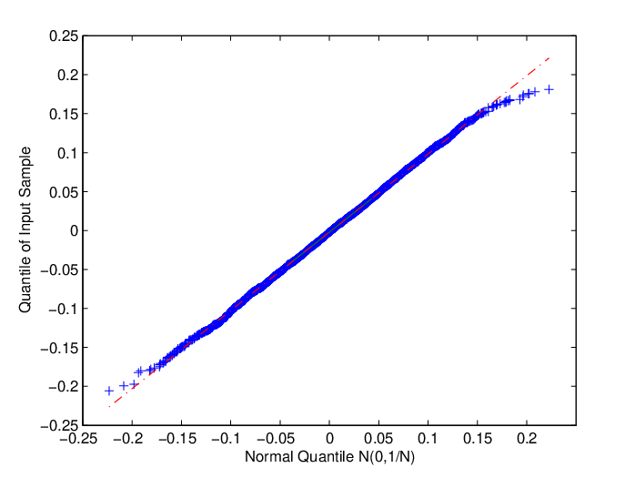
(b)
Note that is a submatrix of . Thus, asymptotical distribution of the entries of is similar to that of entries of .
Before presenting the asymptotical theoretical analysis, we introduce the following assumptions for the local and global randomization models.
III-A1 Assumptions for the Local Randomization Model
- •
is an unit-norm row matrix with absolute magnitude of all entries on the order of .
- •
is an unit-norm column matrix with the maximal absolute magnitude of entries on the order of .
III-A2 Assumptions for the Global Randomization Model
The global randomization model requires similar assumptions for the local randomization model plus the following extra assumptions
- •
The average sum of entries on each column of is on the order of .
- •
Sum of entries on each row of is zero.
- •
Entries on each row of and on each column of are not all equal.
Theorem III.1.
Let , where is the local randomizer. Given the assumptions for the local randomization model, entries of are asymptotically normally distributed with .
Proof.
With notations being defined in Section II-B, we have:
| (4) |
Denote . Because are i.i.d Bernoulli random variables, are i.i.d zero-mean random variables with . The assumption that are on the order of implies that there exist two positive constants and such that:
| (5) |
The variance of , , can be bounded as the follows:
| (6) |
Because is a sum of i.i.d zero-mean random variables , according to the Central Limit Theorem (CLT)(see Appendix A), . To apply CLT, we need to verify its convergence condition: for a given and there exists that is sufficiently large such that the satisfy:
| (7) |
To show that this convergence condition is met, we use the counterproof method. Assume there exists such that , there exists at least :
| (8) |
This inequality can not be true if is on the order of . The underlying intuition of the convergence condition is to guarantee that there is no random variable with dominant variance in the sum . In this case, it simply requires that there is no dominant entry on each column of . ∎
Similarly, we can obtain a similar result when is a uniformly random permutation matrix.
Theorem III.2.
Let , where is the global randomizer. Given the assumptions for the global randomization model, entries of are asymptotically normally distributed , where .
Proof.
Let be a uniform random permutation of . Note that can be viewed as a sequence of random variables with identical distribution. In particular, for a fixed :
Denote (we omit the dependence of on and to simplify the notation), we have:
Using the assumption that the vector has zero average sum and unit norm, we derive:
and also,
In addition, note that although have the identical distribution, they are correlated random variables because of the uniformly random permutation without replacement. Thus, with a pair of and such that , we have:
The last equation holds because the vector has zero average sum and unit-norm. Then, we derive the expectation and the variance of as follows:
The forth equations holds because the column has unit-norm. The theorem is then a simple corollary of the Combinatorial Central Limit Theorem [20] (see Appendix ), provided that its convergence condition can be verified that is:
| (10) |
where
Because , and , the equation (10) holds if the following equation holds:
| (11) |
Because are on the order of :
| (12) |
Also, due to and are on the order of :
| (13) |
The condition that each row of has zero average sum is to guarantee that entries of have zero mean while the condition that entries on each row of and on each column of are not all equal is to prevent the degenerate case that entries of might become a deterministic quantity. For example, when entries of a row are all equal , , which is a deterministic quantity, not a random variable. Note that these conditions are not needed when is the local randomizer.
If is a DCT matrix, a (normalized) WHT matrix or a (normalized) DFT matrix, all the rows (except for the first one) have zero average sum due to the symmetry in these matrices. The first row, whose entries are all equal , can be considered as the averaging row, or a lowpass filtering operation. When the input signal is zero-mean, this row might be chosen or not without affecting quality of the reconstructed signal. Otherwise, it should be included in the chosen row set to encode the signal’s mean. Lastly, the condition that absolute average sum of every column of the sparsifying basis are on the order of is also close to the reality because the majority of columns of the sparsifying basis can be roughly viewed as bandpass and highpass filters whose average sum of the coefficients are always zero. For example, if is a wavelet basis (with at least one vanishing moment), then all columns of (except one at DC) has column sum of zero.
The aforementioned theorems show that under certain conditions, the majority of entries of (also ) behave like Gaussian random variables , where ). Roughly speaking, this behavior constitutes to a good sensing performance for the proposed framework. However, these asymptotic results are not sufficient for establishing sensing performance analysis because in general, entries of are not stochastically independent, violating a condition of a sensing Gaussian i.i.d matrix. In fact, the sensing performance might be quantitatively analyzed by employing a powerful analysis framework of a random subset of rows of an orthonormal matrix [14]. Note that is also an orthonormal matrix when is the local or the global randomizer.
Based on the Gaussian tail probability and a union bound for the maximum absolute value of a random sequence, the maximum absolute magnitude of can be asymptotically bounded as follows:
where and is some positive constant and stands for ”asymptotically smaller or equal”, i.e., when goes to infinity, becomes .
If we choose , the above inequality is equivalent to:
which implies that with probability at least , the mutual
coherence of and is upper bounded by
, which is close to
the optimal bound, except the factor.
In the following section, we will employ a more powerful tool from the theory of concentration inequalities to analyze the coherence between and when is finite. We also consider a more general case that is a sparse matrix (e.g. a block-diagonal matrix).
III-B Incoherence Analysis
Before presenting theoretical results for incoherence analysis, we introduce assumptions for block-based local and global randomization models.
III-B1 Assumptions for the Block-based Local Randomization Model
- •
is an unit-norm row matrix with the maximal absolute magnitude of entries on the order of , where , i.e. , where is some positive constant.
- •
is an unit-norm column matrix.
III-B2 Assumptions for the Block-based Global Randomization Model
The block-based global randomization model requires similar assumptions for the block-based local randomization model plus the following assumption:
- •
All rows of have zero average sum.
Theorem III.3.
Let , where is the local randomizer. Given the assumptions for the block-based local randomization model, then
- •
With probability at least , the mutual coherence of and is upper bounded by .
- •
In addition, if the maximal absolute magnitude of entries of is on the order of , the mutual coherence is upper bounded by , which is independent of .
Proof.
A common proof strategy for this theorem as well as for other theorems in this paper is to establish a large deviation inequality that implies the quantity of our interest is concentrated around its expected value with high probability. Proof steps include:
- •
Showing that the quantity of our interest is a sum of independent random variables;
- •
Bounding the expectation and variance of the quantity;
- •
Applying a relevant concentration inequality of a sum of random variables;
- •
Applying a union bound for the maximum absolute value of a random sequence.
In this case, the quantity of interest is:
Denote , for (in the support set of the row ). Because are i.i.d Bernoulli random variables, are also i.i.d random variables with . are also bounded because
is a sum of independent, bounded random variables. Applying the Hoeffding’s inequality (see Appendix 2) yields:
The next step is to evaluate . Here, can be roughly viewed as the approximation of the variance of .
| (14) |
If the maximal absolute magnitude of entries of is on the order of :
where is some positive constant, then
| (15) |
Finally, we derive an upper bound of the mutual coherence by taking a union bound for the maximum absolute value of a random sequence:
Choose , after simplifying the inequality, we get:
Thus, with an arbitrarily , (14) holds and we achieve the first claim of the Theorem:
Remark III.1.
When is some popular transform such as the DCT or the normalized WHT, the maximal absolute magnitude of entries is on the order of . As a result, the mutual coherence of and an arbitrary is upper bounded by , which is also consistent with our asymptotic analysis above. In other words, when at least or is a dense and uniform matrix, i.e. the maximal absolute magnitude of their entries is on the order of , their mutual coherence approaches the minimal bound, except for the factor. In general, the mutual coherence between an arbitrary and a sparse matrix (e.g. block diagonal matrix of block size ) might be times larger.
Cumulative coherence is another way to quantify incoherence between two matrices [21].
Definition III.1.
The cumulative coherence of an matrix and an matrix is defined as:
where and are rows of and columns of , respectively.
The cumulative coherence measures the average incoherence between two matrices and while mutual coherence measures the entry-wise incoherence. As a result, the cumulative coherence seems to be a better indicator of average sensing performance. In many cases, we are only interested in cumulative coherence between and , where is the support of the transform coefficient vector. As will be shown in the following section, the cumulative coherence provides a more powerful tool to obtain a tighter bound for the number of measurements required for exact recovery.
From the definition of cumulative coherence, it is easy to verify that . If we directly apply the result of the Theorem III.3, we obtain a trivial bound of the cumulative coherence: for an arbitrary basis and for a dense and uniform . In fact, we can get rid of the factor by directly measuring the cumulative coherence from its definition.
Theorem III.4.
Let , where is the local randomizer. Given the assumptions for the block-based local randomization model, with probability at least , the cumulative coherence of and , where , is upper bounded by .
Proof.
Denote and are columns of . Let and () be rows of and columns of , respectively.
Denote and is the matrix of columns , . First, we derive upper bound for the Frobenius norm of :
The last equation holds because . Also, the bound for the spectral norm is:
The last equation holds because . Now, we have:
Let us denote .
is a Rademacher sum of vectors and is a random variable. To show that is concentrated around its expectation, we first derive bound of . It is easy to verify that for a random variable , . Thus, we will derive the upper bound for the simpler quantity
The third equality holds because are i.i.d Bernoulli random variables and thus, . As a result,
Applying Ledoux’s concentration inequality of the norm of a Rademacher sum of vectors [22] (see Appendix 2). Noting that can be viewed as the variance of , yields:
Finally, apply a union bound for the maximum absolute value of a random process,we obtain:
Choose , we get:
Finally, we derive:
∎
Remark III.2.
When , the cumulative coherence is upper bounded by . When , the upper bound of the cumulative coherence is , which is similar to that of the mutual coherence in Theorem III.3.
Remark III.3.
When is some popular transform such as the DCT or the normalized WHT, the maximum absolute magnitude of entries is on the order of . As a result, the cumulative coherence of and any arbitrary ,where , is upper bounded by if .
Remark III.4.
The above theorem represents the worst-case analysis because can be an arbitrary matrix (the worst case corresponds to the case when is the identity matrix). When is known to be dense and uniform, the upper bound of cumulative coherence, according to the Theorem III.3 and the fact that , is , which is, in general, better than .
The asymptotical distribution analysis in Section III-A reveals a significant technical difference required for two randomization models. With the local randomizer, entries of are sums of independent random variables while with the global randomizer, they are sums of dependent random variables. Stochastic dependence among random variables makes it much harder to set up similar arguments of their sum’s concentration. In this case, we will show that the incoherence of and might depend on an extra quantity, the heterogeneity coefficient of the matrix .
Definition III.2.
Assume is an matrix. Let be the support of the column . Define:
| (16) |
The column-wise heterogeneity coefficient of the matrix is defined as:
| (17) |
Obviously, . illustrates the difference between the largest entry’s magnitude and the average energy of nonzero entries. Roughly speaking, it indicates heterogeneity of nonzero entries of the vector . If nonzero entries of a column are homogeneous, i.e. they are on the same order of magnitude, is on the order of a constant. If all nonzero entries of a matrix are homogeneous, the heterogeneity coefficient is also on the order of a constant, and is referred as a uniform matrix. Note that a uniform matrix is not necessarily dense, for example, a block-diagonal matrix of DCT or WHT blocks
The following theorem indicates that when the global randomizer is employed, the mutual coherence between and is upper-bounded by , where is the block size of and is an arbitrarily matrix with the heterogeneity coefficient .
Theorem III.5.
Let , where is the global randomizer. Assume that , where is defined as in (16). Given the assumptions for the block-based global randomization model, then
- •
With probability at least , the mutual coherence of and is upper-bounded by , where is defined as in (17)
- •
In addition, if is dense and uniform, i.e. the maximum absolute magnitude of its entries is on the order of and , the mutual coherence is upper-bounded by , which is independent of .
Proof.
Let be a uniformly random permutation of .
As in the proof of the Theorem III.2, can be viewed as a sequence of dependent random variables with identical distribution, i.e. for a fixed :
The condition of is equivalent to , where is some positive constant. Define as the follows:
It is easy to verify that . Define as the sum of dependent random variables
Note that are zero-mean random variables because has zero average sum. Thus, and . Then, applying the Sourav’s theorem of concentration inequality for a sum of dependent random variables [23] (see Appendix 2) results in:
Denote . The above inequality is equivalent to:
By choosing , we achieve:
If , the denominator inside the exponent is smaller than . Thus,
Finally, after taking the union bound for the maximum absolute value of a random sequence and simplifying the inequality, we obtain the first claim of the Theorem:
If is known to be dense and uniform, i.e. , where is some positive constant. We then define as the following:
Note that and . Repeat the same arguments above, we have:
Similarly, choose , we can derive:
If , the denominator inside the exponent is smaller than . Thus,
After taking the union bound of the maximum absolute value of a random sequence, we achieve the second claim of the Theorem. ∎
Remark III.5.
The first part of theorem implies that when is a dense and uniform matrix (e.g. DCT or normalized WHT) and is a uniform matrix (not necessarily dense), the mutual coherence closely approaches the minimum bound . Although in this theorem, the mutual coherence depends on the heterogeneity coefficient, one will see in the experimental Section V that this dependence is almost negligible in practice.
As a consequence of this theorem, when at least or is dense and uniform, the mutual coherence of and is roughly on the order of , which is quite close to the minimal bound , except for the factor. Otherwise, the coherence linearly depends on the block size of and is on the order of . As a matter of fact, this bound is almost optimal because when is the identity matrix, the mutual coherence is actually equal the maximum absolute magnitude of entries of , which is on the order of .
Remark III.6.
Although the theoretical results of the global randomizer seem to be always weaker than those of the local randomizer, there are a few practical motivations to study this global randomizer. Speech scrambling has been used for a long time for secure voice communication. Also, analog image/video scrambling have been implemented for commercial security related applications such as CCTV surveillance system. In addition, permutation does not change the dynamic range of the sensing signal, i.e. no bit expansion in implementation. The computation cost of random permutation is only , which is very easy to implement in software. From a security perspective the operation of random permutation offers a large key space than random sign flipping ( vs ). Also, as will be shown in the numerical experiment section, with random permutation, one can get highly sparse measurement matrix.
IV Compressive Sampling Performance Analysis
Section III demonstrates that under some mild conditions, the matrix and are highly incoherent, implying that the matrix is almost dense. When is dense, energy of nonzero transform coefficients is distributed over all measurements. Commonly speaking, this is good for signal recovery from a small subset of measurements because if energy of some transform coefficients were concentrated in few measurements that happens to be bypassed in the sampling process, there is no hope for exact signal recovery even when employing the most sophisticated reconstruction method. This section shows that a random subset of rows of the matrix yields almost optimal measurement matrix for compressive sensing.
IV-A Assumptions for Performance Analysis
A signal is assumed to be sparse in some sparsifying basis : , where the vector of transform coefficients has no more than nonzero entries. The sign sequence of nonzero transform coefficients which is denoted as , is assumed to be a random vector of i.i.d Bernoulli random variables (i.e. ). Let be the measurement vector, where is a Structurally Random Matrix. Assumptions of the block-based local randomization and of the block-based global randomization models hold.
IV-B Theoretical Results
Theorem IV.1.
With probability at least , the proposed sensing framework can recover -sparse signals exactly if the number of measurements . If is a dense and uniform rather than block-diagonal(e.g. DCT or normalized WHT matrix), the number of measurement needed is on the order of .
Proof.
Remark IV.1.
If is dense and uniform, the number of measurements for exact recovery is always regardless of the block size . This implies that we can use the identity matrix for the transform (B = 1). For example, when the input signal is known to be spectrally sparse, compressively sampling it in the time domain is as efficient as in any other transform domain.
Compared with the framework that uses random projection, there is an upscale factor of for the number of measurements for exact recovery. In fact, by employing the bound of cumulative coherence, we can eliminate this upscale factor and thus, successfully showing optimal performance guarantee.
Theorem IV.2.
Assume that the sparsity . With probability at least , the proposed framework employing the local randomizer can reconstruct -sparse signals exactly if the number of measurements .If is a dense and uniform matrix (e.g. DCT or normalized WHT), the minimal number of required measurements is .
Proof.
The proof is based on the result of cumulative coherence in the Theorem III.4 and a modification of the proof framework of the compressed sensing [14].
Denote , , and , where the support . Let , , be columns of . Denote , where is the cumulative coherence of and . According to the above incoherence analysis, . Also, denote as the mutual coherence of and , .
As indicated in [12, 14], to show minimization exact recovery, it is sufficient to verify the Exact Recovery Principle.
Exact Recovery Principle.
With high probability, for all , where is the complementary set of the set and , where is the sign vector of nonzero transform coefficients .
Note that , where is the row of , for some . To establish the Exact Recovery Principle, we will first derive following lemmas. The first lemma is to bound the norm of .
Lemma IV.1.
(Bound the norm of ) With high probability, is on the order of :
where , and are some certain numbers.
Proof.
Let be columns of . For :
where the second equality holds because that results from the orthogonality of columns of . Let . Because are i.i.d binary random variables with , are zero mean i.i.d random variables and . Let be the matrix of columns , . Then, can be viewed as a random weighted sum of column vectors :
and is a random variable. We have:
where the last equality holds due to if . Thus,
where the last inequality holds due to . This implies that . To show that is concentrated around its mean, we use the Talagrand’s theorem of concentration inequality [24]. First, we have:
where the last equation holds because . Thus, we derive the upper bound of the variance :
In addition, it is obvious that and thus
The Talagrand’s theorem [24] (see Appendix 2) shows that:
where is some positive constant. Replacing , and by their upper bounds in the right-hand side, we obtain:
The next step is to simplify the right-hand side of the above inequality by replacing the denominator inside the by two times the dominant term and note that when . In particular, there are two cases:
- •
Case 1: or equivalently, , denote and . If or equivalently, ,
- •
Case 2: , denote and . If or equivalently,
where is some positive constant.
In conclusion, let . Then, for any :
| (18) |
where is some positive constant. ∎
The second lemma is to bound the spectral norm of
Lemma IV.2.
(Bound the spectral norm of )
With high probability,
Proof.
The Theorem in [14] shows that with probability , if , where and are some known positive constants.
∎
And the third lemma is to bound the norm of
Lemma IV.3.
(Bound the norm of )
With high probability, is on the order of :
| (19) |
where , and are defined in the proof of the Lemma IV.1.
Proof.
Let be the event that or equivalently, and be the event that . Note that
Thus,
Note that implies (19) holds.
∎
To establish the Exact Recovery Principle, we will show that with high probability. Note that because is assumed to be a vector of i.i.d Bernoulli random variables, is concentrated around its zero mean. In particular, according to the Hoeffding’s inequality:
Note that with two arbitrary probabilistic events and :
Now, let be the event and be the event , we derive
| (20) |
Choose , according to (19) and (20), the probability of our interest is upper bounded by:
To show that with probability , it is sufficient to show that the above upper bound is not greater than . In particular, choose that makes the first term to be equal .
To make the second term less than , it is required that
| (21) |
- •
- •
In conclusion, the Exact Recovery Principle is verified if , where and are known positive constants.
Finally, note that and and the assumption that , the sufficient condition for exact recovery is . When is dense and uniform, the condition becomes .
∎
V Numerical Experiments
V-A Simulation with Sparse Signals
In this section, we evaluate the sensing performance of several structurally random matrices and compare it with that of the completely random projection. We also explore the connection among sensing performance (probability of exact recovery), streaming capacity (block size of ) and structure of the sparsifying basis (e.g. sparsity and heterogeneity).
In the first simulation, the input signal of length is sparse in the DCT domain, i.e. , where the sparsifying basis is the IDCT matrix. Its transform coefficient vector has nonzero entries whose magnitudes are Gaussian distributed and locations are at uniformly random, where . With the signal , we generate a measurement vector of length : , where is some structurally random matrix or a completely Gaussian random matrix. SRMs under consideration are summarized in Table I.
| Notation | R | F |
|---|---|---|
| WHT64-L | Local randomizer | block diagonal WHT |
| WHT64-G | Global randomizer | block diagonal WHT |
| WHT256-L | Local randomizer | block diagonal WHT |
| WHT256-G | Global randomizer | block diagonal WHT |
The software -magic [1] is employed to recover the signal from its measurements . For each value of sparsity , we repeat the experiment 500 times and count the probability of exact recovery. The performance curve is plotted in Fig. 2(a). Numerical values on the -axis denote signal sparsity while those on the -axis denote the probability of exact recovery. We then repeat similar experiments when an input signal is sparse in some sparse and non-uniform basis . Fig. 2(b) and Fig. 2(c) illustrate the performance curves when is the Daubechies-8 wavelet basis and the identity matrix, respectively.
There are a few notable observations from these experimental results. First, performance of the SRM with the dense transform matrix (all of its entries are non-zero) is in average comparable to that of the completely random matrix. Second, performance of the SRM with the sparse transform matrix , however, depends on the sparsifying basis of the signal. In particular, if is dense, the SRM with sparse also has average performance comparable with the completely random matrix. If is sparse, the SRM with sparse often has worse performance the SRM with dense , revealing a trade-off between sensing performance and streaming capacity. These numerical results are consistent with the theoretical analysis above. In addition, Fig. 2(b) shows that the SRM with the global randomizer seems to work much better than the SRM with the local randomizer when the sparsifying basis of the signal is sparse.

(a)

(b)

(c)
V-B Simulation with Compressible Signals
In this simulation, signals of interest are natural images of size such as the Lena, Barbara and Boat images. The sparsifying basis used for these natural images is the well-known Daubechies wavelet transform. All images are implicitly regarded as 1-D signals of length . The GPSR software in [3] is used for signal reconstruction.
For such a large scale simulation, it takes a huge amount of system resources to implement the sensing method of a completely random matrix. Thus, for the purpose of benchmark, we adopt a more practical scheme of partial FFT in the wavelet domain (WPFFT). The WPFFT is to sense wavelet coefficients in the wavelet domain using the method of partial FFT. Theoretically, WPFFT has optimal performance as the Fourier matrix is completely incoherent with the identity matrix. The WPFFT is a method of sensing a signal in the transform domain that also requires substantial amount of system resources. SRMs under consideration are summarized in Table II.
| Notation | R | F |
|---|---|---|
| DCT32-G | Global randomizer | block diagonal DCT |
| WHT32-G | Global randomizer | block diagonal WHT |
| DCT512-L | Local randomizer | block diagonal DCT |
| WHT512-L | Local randomizer | block diagonal WHT |
For the purpose of comparison, we also implement two popular sensing methods: partial FFT in the time domain (PFFT)[1] and the Scrambled/Permutted FFT (SFFT) in [25, 26] that is equivalent to the dense SRM using the global randomizer.
The performance curves of these sensing ensembles are plotted in Fig. 3(a), Fig. 3(b) and Fig. 3(c), which correspond to the input signal Lena, Barbara and Boat images, respectively. Numerical value on the -axis represents sampling rate, which is the number of measurements over the total number of samples. Value on -axis is the quality of reconstruction (PSNR in dB). Lastly, Fig. 4 shows the visually reconstructed Boat image from of measurements using WPFFT, WHT32-G and WHT512-L ensembles.

(a)

(b)

(c)
As clearly seen in Fig. 3, the PFFT is not an efficient sensing matrix for smooth signals like images because Fourier matrix and wavelet basis are highly coherent. On the other hand, the SRM method, which can roughly be viewed as the PFFT preceded by the pre-randomization process, is very efficient. In particular, with a dense SRM like SFFT, the performance difference between the SRM method and the benchmark one, WPFFT, is less than dB. In addition, performance of DCT512-L and WHT512-L that are fully streaming capable SRM, degrades about dB, which is a reasonable sacrifice as the buffer size required is less than percent of the total length of the original signal. Less degradation is obtainable when the buffer size is increased. Also, in all cases, there is no observable difference of performance between DCT and normalized WHT transforms. It implies that orthonormal matrices whose entries have the same order of absolute magnitude generate comparable performance. In addition, highly sparse SRM using the global randomizer such as DCT32-G and WHT32-G has experimental performance comparable to that of the dense SRMs. Note that these SRM are highly sparse because their density are only . This observation again verifies that SRM with the global randomizer outperforms SRM with the local randomizer. This might indicate that our theoretical analysis for the global randomizer is inadequate. In practice, we believe that the global randomizer always works as well as and even better than the local randomizer. We leave the theoretical justification of this observation for our future research.


VI Discussion and Conclusion
VI-A Complexity Discussion
We compare the computation and memory complexity between the proposed SRM and other random sensing matrices such as Gaussian or Bernoulli i.i.d. matrices. In implementation, the i.i.d Bernoulli matrix is obviously preferred than i.i.d Gaussian one as the former has integer entries and requires only 1 bit to represent each entry. A i.i.d. Bernoulli sensing matrix requires bits for storing the matrix and additions and multiplications for sensing operation. An SRM only requires bits for storage and additions and multiplications for sensing operation. With the SRM method, the computational complexity and memory space required is independent with the number of measurements . Note that with the SRM method, we do not need to store matrices , , explicitly. We only need to store the diagonals of and of and the fast transform , resulting in significant saving of both memory space and computational complexity.
Computational complexity and running time of -minimization based reconstruction algorithms often depend critically on whether matrix-vector multiplications and can be computed quickly and efficiently (where ) [3]. For the sake of simplicity, assuming that is identity matrix. requires additions and multiplications for a random sensing matrix and additions and multiplications for the SRM method. This implies that at each iteration, SRM can speed up the reconstruction algorithm with at least folds. With compressible signals (e.g., images), the number of measurements acquired tends to be proportional with the signal dimension, for example, . In this case, using SRM can achieve computational complexity reduction with the factor of times.
Table III summarizes computational complexity and practical advantages between SRM and a random sensing matrix.
| Features | SRMs | Completely Random Matrices |
|---|---|---|
| No. of measurements for exact recovery | ||
| Sensing complexity | ||
| Reconstruction complexity at each iteration | ||
| Fast computability | Yes | No |
| Block-based processing | Yes | No |
VI-B Relationship with Other Related Works
When is the local randomizer, SRM is a little reminiscent to the so-called Fast Johnson-Lindenstrauss Transform (FJLT) [27]. However, SRM employs a simpler matrix . In FJLT, this matrix is a completely random matrix with sparse distribution. It is unknown if there exists an efficient implementation of such a sparse random matrix. SRM is relevant for practical applications because of its high performance and fast computation.
In [25, 26], the Scrambled/Permuted FFT is experimentally proposed as a heuristic low-complexity sensing method that is efficient for sensing a large signal. To the best of our knowledge, however, there has not been any theoretical analysis for the Scrambled FFT. SRM is a generalized framework in which Scrambled FFT is just a specific case, and thus verifying the theoretical validity of the Scrambled FFT.
Random Convolution convolving the input signal with a random pulse followed by randomly subsampling measurements is proposed in [19] as a promising sensing method for practical applications. Although there are a few other methods that exploit the same idea of convolving a signal with a random pulse, for examples: Random Filter in [17] and Toeplitz structured sensing matrix in [18], only the Random Convolution method can be shown to approach optimal sensing performance. While sensing methods such as Random Filter and Toeplitz-based CS methods subsample measurements structurally, the Random Convolution method subsamples measurements in a random fashion, a technique that is also employed in SRM. In addition, the Random Convolution method introduces randomness into the Fourier domain by randomizing phases of Fourier coefficients. These two techniques decouple stochastic dependence among measurements and thus, giving the Random Convolution method a higher performance.
SRM is distinct from all aforementioned methods, including the Random Convolution one. A key difference is that SRM pre-randomizes a sensing signal directly in its original domain (via the global randomizer or the local randomizer) while the Random Convolution method pre-randomizes a sensing signal in the Fourier domain. SRM also extends the Random Convolution method by showing that not only Fourier transform but also other popular fast transforms, such as DCT or WHT, can be employed to achieve similar high performance. In conclusion, among existing sensing methods, the SRM framework presents an alternative approach to design high performance, low-complexity sensing matrices with practical and flexible features.
Appendix A
Central Limit Theorem.
Let be mutually independent random variables. Assume and denote . If for a given and sufficiently large, the following inequalities hold:
then distribution of the normalized sum converges to
Combinatorial Central Limit Theorem.
Given two sequences and . Assume the are not all equal and are also not all equal. Let be a uniform random permutation of . Denote and
is asymptotically normally distributed if
where
Appendix B
Hoeffding’s Concentration Inequality.
Suppose are independent random variables and (). Define a new random variable . Then for any
Ledoux’s Concentration Inequality.
Let be a sequence of independent random variables such that almost surely and , ,…, be vectors in Banach space. Define a new random variable: . Then for any ,
where denote the variance of and .
Talagrand’s Concentration Inequality.
Let be zero-mean i.i.d random variables and bounded and be column vectors of a matrix . Define a new random variable: . Then for any :
where is some constant, variance and .
Sourav’s Concentration Inequality.
Let be a collection of numbers from . Let be a uniformly random permutation of . Define a new random variable: . Then for any
References
- [1] E. Candès, J. Romberg, and T. Tao, “Robust uncertainty principles: Exact signal reconstruction from highly incomplete frequency information,” IEEE Trans. Inf. Theory, vol. 52, pp. 489 – 509, 2006.
- [2] D. L. Donoho, “Compressed sensing,” IEEE Trans. Inf. Theory, vol. 52, no. 4, pp. 1289 – 1306, 2006.
- [3] M. A. T. Figueiredo, R. D. Nowak, and S. J. Wright, “Gradient projection for sparse reconstruction,” IEEE J. Sel. Topics Signal Process., vol. 1, no. 4, pp. 586–597, 2007.
- [4] E. T. Hale, W. Yin, and Y. Zhang, “Fixed-point continuation for l-minimization: Methodology and convergence,” SIAM J. Opt., vol. 19, no. 3, pp. 1107–1130, 2008.
- [5] E. V. D. Berg and M. P. Friedlander, “Probing the pareto frontier for basis purusit solutions,” SIAM J. Scien. Comp., vol. 31, no. 2, pp. 890–912, 2008.
- [6] J. Tropp and A. Gilbert, “Signal recovery from random measurements via orthogonal matching pursuit,” IEEE Trans. Info. Theory, vol. 53, no. 12, pp. 4655–4666, Dec 2007.
- [7] D. Needell and J. A. Tropp, “Cosamp: Iterative signal recovery from incomplete and inaccurate samples,” Appl. Comput. Harmon. Anal., vol. 26, pp. 301–321, 2008.
- [8] W. Dai and O. Milenkovic, “Subspace pursuit for compressive sensing signal reconstruction,” IEEE Trans. Inf. Theory, vol. 55, no. 5, pp. 2230–2249, 2009.
- [9] D. L. Donoho, Y. Tsaig, and J.-L. Starck, “Sparse solution of underdetermined linear equations by stagewise orthogonal matching pursuit,” Technical Report, 2006.
- [10] T. T. Do, L. Gan, N. Nguyen, and T. D. Tran, “Sparsity adaptive matching pursuit algorithm for practical compressed sensing,” Asilomar Conf. Sign. Sys. Comput., pp. 581–587, 2008.
- [11] D. L. Donoho and X. Huo, “Uncertainty principles and ideal atomic decomposition,” IEEE Trans. Inf. Theory, vol. 47, no. 7, pp. 2845 – 2862, 2001.
- [12] E. Candès and T. Tao, “Near optimal signal recovery from random projections: Universal encoding strategies?,” IEEE Trans. Inf. Theory, vol. 52, no. 12, pp. 5406 – 5425, 2006.
- [13] S. Mendelson, A. Pajor, and N. Tomczak-Jaegermann, “Uniform uncertainty principle for bernoulli and subgaussian ensembles,” Constructive Alg., vol. 28, pp. 269–283, 2008.
- [14] E. Candès and J. Romberg, “Sparsity and incoherence in compressive sampling,” Inverse Problems, vol. 23, no. 3, 2007.
- [15] R. Coifman, F. Geshwind, and Y. Meyer, “Noiselets,” Appl. Comput. Harmon. Anal., vol. 10, pp. 27–44, 2001 2005.
- [16] E. Candès and T. Tao, “Decoding by linear programming,” IEEE Trans. Inf. Theory, vol. 51, no. 12, pp. 4203–4215, 2005.
- [17] J. Tropp, M. Wakin, M. Duarte, D. Baron, and R. Baraniuk, “Random filters for compressive sampling and reconstruction,” IEEE Conf. Acous. Speech Sign. Proc., vol. 3, pp. 872–875, 2006.
- [18] W. Bajwa, J. Haupt, G. Raz, S. Wright, and R. Nowak, “Toeplitz-structured compressed sensing matrices,” IEEE Stat. Sign. Proc. (SSP), pp. 26–29, 2007.
- [19] J. Romberg, “Compressive sensing by random convolution,” SIAM J. Imaging Sci., vol. 2, pp. 1098–1128, 2009.
- [20] W. Hoeffding, “A combinatorial central limit theorem,” The Annals Math. Stat., vol. 22, pp. 558–566, 1951.
- [21] K. Schnass and P. Vandergheynst, “Average performance analysis for thresholding,” IEEE Sign. Proc. Letters, vol. 14, no. 11, 2007.
- [22] M. Ledoux, “The concentration of measure phenomenon,” American Mathematical Society, 2001.
- [23] S. Chatterjee, “Stein’s method for concentration inequalities,” Probab. Theory Related Fields, vol. 138, pp. 305–321, 2007.
- [24] M. Talagrand, “New concentration inequalities in product spaces,” Invent. Math., vol. 126, pp. 505–563, 1996.
- [25] E. Candès, J. Romberg, and T. Tao, “Stable signal recovery from incomplete and inaccurate measurements,” Comm. Pure Applied Math., vol. 59, no. 8, 2006.
- [26] M. F. Duarte, M. B. Wakin, and R. G. Baraniuk, “Fast reconstruction of piecewise smooth signals from incoherent projections,” Workshop Sign. Proc. Adapt. Sparse Struc. Represent., 2005.
- [27] N. Ailon and B. Chazelle, “Approximate nearest neighbors and the fast johnson-lindenstrauss transform,” Proc. 38th ACM Symp. Theory Comput., vol. 66, pp. 557 – 563, 2006.