Perfect State Transfer in Two and Three Dimensional Structures
Abstract
We introduce a scheme for perfect state transfer in regular two and three dimensional structures. The interactions on the lattices are of XX spin type with uniform couplings. In two dimensions the structure is a hexagonal lattice and in three dimensions it consists of hexagonal planes joined to each other at arbitrary points. We will show that compared to other schemes, i) much less control is needed for routing, ii) the algebra of global control is quite simple, iii) the same kind of control can upload and download qubit states to or from built-in Read-Write (RW) heads. Pivotal use is made of a quantum switch which we introduce and call it Hadamard switch, since its operation depends on the existence of a Hadamard matrix in four dimensions.
Introduction: Since the inception of the fields of quantum information and computation, the task of coherently transferring quantum states, through long and short distances has been of utmost importance. While photons are the ideal carriers of quantum information over long distances, it has become evident that the best possible method for transferring quantum information over short distances, i.e. through regular arrays of qubits, is to exploit the natural dynamics of the many body system. This idea was first introduced in the work of Bose [1] who showed that the natural dynamics of a Heisenberg ferromagnetic chain can achieve high-fidelity transfer of qubits over distances as long as 80 lattice units.
In contrast to the traditional passive view in the study of many body dynamics, where the dynamics is only calculated and observed, this has led to an active view in the dynamics of solid state systems, where we intervene in the dynamics to achieve certain goals. For example it is tried to engineer the couplings in such a way that states are transferred with perfect [2, 3] or with arbitrary high fidelity [4, 5, 6, 7, 8, 9], or it is tried to interrupt the natural evolution by some minimal control to achieve this task [11, 12, 13, 14].
To overcome the necessity of engineered couplings, which severely restricts experimental realization of such protocols, some kind of control was re-introduced in the scheme [15], wherre it was shown in [15] that quasi one dimensional chains with uniform couplings, can achieve perfect transfer. Conversion of these linear structures to star configurations [15] and arranging them in 2 dimensional structures was shown to achieve perfect state transfer in two and higher dimensions. However the nature of subsystems introduced in [15] required multiple control on external nodes of each subsystem, and different types of control for matching subsystems with each other. A different type of control was also necessary for loading and extracting the states to or from the lattice.
In this letter we introduce a very simple scheme for perfect
transfer, in two and three dimensional lattices. In addition to
having all the nice properties of the protocol of
[15], like linear scaling of time with distance, and
robustness to errors, this scheme has very desirable extra
properties, namely:
i) very simple global operations are needed for routing
arbitrary states through arbitrary paths, that is, to each route
a very simple sequence of operations corresponds,
ii) the lattice has natural built-in local read-write
(RW) heads for uploading and downloading qubit states,
iii) the same kind of global control which is used for
routing, is also used for uploading and downloading states to or
from input and output heads.
As we will see, all these properties, are based on the geometry
of hexagonal lattice and on a concept (or device) which we
introduce for the first time. We call it the Hadamard switch,
since it uses the four dimensional Hadamard matrix.
In fact in [15], a localized (particle) state in one of the input nodes, is considered as a superposition of complex extended waves on all the input nodes where only one of these waves passes through the star-shaped subsystem to the output nodes and vice versa, while all the other waves are reflected back. Therefore one needs to control the external nodes a few times by applying suitable phase gates so that after multiple traversal and reflections, the waves again interfere constructively to create a particle state on a particular output node. As we will show, the Hadamard switch and its natural embedding in hexagonal lattices improves in a dramatic way all these features. Moreover it naturally allows the imbedding of RW heads in the lattice structure for uploading and downloading of quantum states.
Preliminaries The prototype of many-body systems which has been used in many protocols is the XY spin chain,
| (1) |
This type of interaction preserves spin , and moreover does not evolve the uniform background state of all spin ups, i.e. , where is the total number of qubits in the lattice. This then leads to the simple result that for transferring an arbitrary qubit state like it is enough to perfectly transfer only the state through the lattice. Such a transfer occurs in the single excitation sector which is spanned by states of the form , where means that the single spin in the th place is down (or the local qubit is in the state ). Note that we use the the names single-excitation and single-particle states interchangeably, i.e. by the transfer of a particle through the lattice, we mean transfer of excitation not any actual particle.
It was shown in [2] that a linear XY chain of length N, with engineered local couplings in the form can achieve perfect transfer between any pair of input and output site in time . It was shown in [2] that the only uniformly coupled XY chains which can do perfect transfer are of length 2 and 3 with respective transfer times and (note that we have normalized the coupling in both chains to unity).
The scheme We start with the hexagonal lattice shown in figure (1). Let denote a vertex of the lattice. On the three links connected to this vertex, there are three qubits, which we denote by , and . The vectors , and denote the three vectors directed along the links connected to a vertex. A fourth qubit , called the read-write (RW) head is also connected to this vertex, although the vector does not necessarily mean a vector in the plane and is used only for uniformity of notation. The Hamiltonian which governs the interaction on this system is of the form
| (2) |
where is the local Hamiltonian connecting each vertex to its neighboring links and through these links to the other vertices.
Now we describe the quantum system at each vertex. At each vertex there are four qubits which we denote by , i.e. . These particles are arranged on four different layers so that all the qubits with the same index lie in one layer. In particular the qubits for different ’s lie in the hexagonal plane and the other qubits lie in different layers which we call control layers to distinguish them from the main hexagonal plane. As we will see later, the only control that we need is the possibility of applying uniform magnetic field on each control layer. No control on any individual qubits is necessary. The interaction between all the spins is a simple interaction. Such an interaction conserves the total z-component of spin and hence when the whole lattice is initialized to the state (spin up), transfer of a particle occurs in the single-particle sector. The local Hamiltonian has the simple form
| (3) |
where are the entries of the Hadamard matrix in four dimensions, namely

| (4) |
We remind the reader that a Hadamard matrix is a symmetric real orthogonal matrix all of whose entries have the same absolute value. Such matrices exist only in certain special dimensions. We will elaborate on the importance of this matrix for our scheme later on. In the above matrix the rows and columns are numbered from 0 to 3 from left to right and from top to bottom respectively. Note that the vertex is connected with each of the three links and also the RW head with equal couplings. We call this structure, described by the Hamiltonian a Hadamard switch. As we will see later, it can be used in a very effective way for routing states through two and three dimensional structures. Figure (2) shows this switch. In figure (1) these switches have been depicted as big colored circles at vertices of the hexagonal lattice.

It can be readily verified that the local XY hamiltonian, on spins and , has the following simple action on the single excitation states, where for . This means that when restricted to single particle subspace has the following expression,
| (5) |
This allows us to rewrite the total Hamiltonian in the form
| (6) |
We now consider the four orthogonal states that is
| (7) | |||||
| (8) | |||||
| (9) | |||||
| (10) |
The Hamiltonian can now be rewritten as
| (11) |
Thus as shown in figure (3), in this new basis the Hamiltonian has been decomposed into direct sum of XY spin chains with uniform couplings of length two and three. We now note that such chains are capable of perfect transfer of qubits in times and respectively.
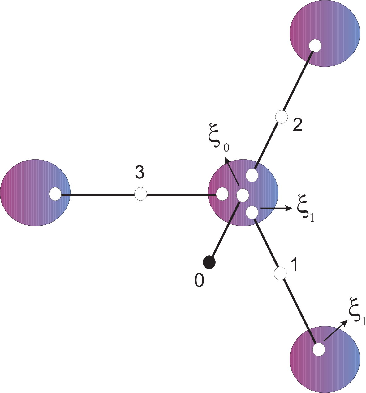
It is important to note that the states are turned into each other by global unitary operators. Let , and be the Pauli operators acting on spins 1, 2 and 3 on vertex . Then it is readily seen that
| (12) | |||
| (13) | |||
| (14) |
The crucial point is that the operations can be applied globally on all the qubits in the control layer, since on the empty sites it has no effect and on an occupied site it has the phase effect that we want. Therefore there is no need for addressing single spins in each control layer, only the possibility of access to each layer is required. Such a control should be applied in a time much shorter than the time scale of evolution of the Hamiltonian, namely and . If we want to route many particles at the same time, we have to control different regions of control layers in accordance with the paths of these particles. The control will be the same in the time intervals when the paths become parallel.
Now a clear and very simple method for perfect state transfer in
the lattice emerges. A single particle is
uploaded to a given input head . The part does
not evolve and indeed is ready for downloading at any output
head. We only have to transfer the single particle state
which in view of our notation, has made the whole lattice to be
in the state . After a time , this state
evolves to , i.e. the particle has moved to
the nearest vertex in the form of a real wave .
Once in a state , we can make a global control
according to (12) to switch this vertex state to
either of the states () depending on the
direction we want to route the state. For example if we switch it
to , then according to figure (3),
after a time , the state will be transferred perfectly to
the vertex in the form . Continuing in
this way we can move the state via any path that we like to any
other vertex say , where the final state will be one of
the three states , (). Switching
this state to will move this state to the
nearest output head in the form where it will
be read off. The total time for routing is , where
is the number of links which connect the input and output heads
along the chosen path. The sequence of control operations is very
simple. For uploading and downloading a qubit to or from a link
to its nearest head, the operation is applied
when means that is removed from the triple
and at each vertex for turning the qubit from link
to link , the operation is applied.
Except for uploading and downloading operations where a time
lapse of is needed all the other control operations are
applied at regular intervals of
time . We restate it as:
for turning from direction to apply ,
For uploading and downloading a qubit to or from a RW
head to direction apply .
Perfect transfer in three dimensions The Hadamard switch can be used in another way for achieving perfect state transfer in three dimensional structures. Figure (2) shows a Hadamard switch connecting two hexagonal planes. Such planes can be joined by any number of switches. The number and positions of Hadamard switches are determined to optimize the accessibility of all the heads in the two planes by shortest possible paths. When used in this new way, the RW head gives its role to the qubit on the link which joins the two planes. For example when the two planes are joined to each other at points , and on the two planes (figure 4), the effective Hamiltonian for the states on the joining link and the states on plane 1 and on the upper plane is nothing but a perfect XY 3-chain. This effective Hamiltonian, transforms the state perfectly between the two planes. This time we should wait for time instead of . Therefore we route a particle within each plane as before and bring it to the position of the nearest switch where by appropriate control we move it to another plane and continue there.
Robustness Like the system in [15], our scheme is also robust against imperfections in the lattice up to a threshold. That is if we know which of the switches are not working we can easily route them around. Moreover due to the very simple nature of the switches and their control, if there is any delay in the control operations, we know exactly on which switch and which link of the switch the particle is waiting. This is due to the fact that under the intrinsic dynamics of the 2 and 3 chains in figure (3), any excitation just goes back and forth between the endpoints of a chain.

Discussion The Hadamard switch introduced in this paper
has a broader applicability than the one presented in this
scheme. In fact, given any type of perfect transfer chain
[2], one can join them by Hadamard switches to each
other and to RW heads to form two and three dimensional
structures for perfect routing of quantum states. In this way one
can use fewer number of switches in each plane and also attach
different planes by longer chains which facilitates the access to
control planes. Compared to the start-structure of
[15], this is achieved at the cost of higher
connectivity in the switch. The main role of this switch, is to
route any single particle from any of its external nodes to any
other simply by single-step control of the central qubits. Were
it not for the existence of a Hadamard matrix in 4 dimensions,
this interesting property could not exist. In fact if one uses any
other matrix instead of the Hadamard, then one looses one or the
other nice property of the switch. For example if one uses a
complex Fourier transform as in [15], then multiple
control is needed on the external nodes, and the waves should
traverse the elementary structures several times until by
suitable control of external nodes, they interfere to form a
particle state at a specific output node. On the other hand if
one uses real orthogonal matrices, then the couplings will no
longer be uniform. It would be interesting to see if the scheme
proposed in this letter can be realized experimentally, in solid
state systems, for example in arrays of Joshephson junctions
[16]. It would also be interesting to see if the
system introduced in this letter can be used as a spin network
quantum computer along the lines set in [17].
Acknowledgement The authors thank Alastair Kay for his valuable comments on an earlier version of this letter. M. A. and V. K. would like to thank L. Memarzadeh for very valuable discussions.
References
- [1] S. Bose, Phys. Rev. Lett. 91, 207901 (2003).
- [2] M. Christandl, N. Datta, A. Ekert, and A. J. Landahl, Phys. Rev. Lett. 92, 187902 (2004). C. Albanese, M. Christandl, N. Datta, and A. Ekert, Phys. Rev. Lett. 93, 230502 (2004). M. Christandl, N. Datta, T. C. Dorlas, A. Ekert, A. Kay, and A. J. Landahl, Phys. Rev. A 71, 032312 (2005).
- [3] C. Di Franco, M. Paternostro, and M. S. Kim, Phys. Rev. Lett. 101, 230502 (2008). M. Markiewicz and M. Wiesniak, Phys. Rev. A 79, 054304 (2009).
- [4] M.B. Plenio and F.L. Semiao, New J. Phys. 7, 73 (2005).
- [5] A. Wojcik, T. Luczak, P. Kurzynski, A. Grudka, T. Gdala, and M. Bednarska, Phys. Rev. A 72, 034303 (2005).
- [6] A. Bayat and S. Bose, Phys. Rev. A 81, 012304 (2010), A. Bayat, L. Banchi, S. Bose and P. Verrucchi, e-print arXiv:1104.0718.
- [7] C. Di Franco, M. Paternostro, and M. S. Kim, Phys. Rev. A 81, 022319 (2010).
- [8] E. B. Fel’dman, E. I. Kuznetsova, and A. I. Zenchuk, Phys. Rev. A 82, 022332 (2010).
- [9] N. Y. Yao, L. Jiang, A. V. Gorshkov, Z.-X. Gong, A. Zhai, L.-M. Duan, and M. D. Lukin, Phys. Rev. Lett. 106, 040505 (2011). N. Y. Yao, L. Jiang, A. V. Gorshkov, P. C. Maurer, G. Giedke, J. Ignacio Cirac, M. D. Lukin, arXiv:1012.2864v1.
- [10] J. Fitzsimons and J. Twamley, Phys. Rev. Lett. 97, 090502 (2006).
- [11] D. Burgarth, S. Bose, and V. Giovannetti, J. Phys. A: Math. Gen. 38, 6793 (2004). D. Burgarth, and S. Bose, Phys. Rev. A 71, 052315 (2005). D. Burgarth, V. Giovannetti and S. Bose, Phys. Rev. A 75, 062327 (2007).
- [12] T. J. Osborne and N. Linden, Phys. Rev. A 69, 052315 (2004).
- [13] P. Cappellaro, C. Ramanathan, and D. G. Cory, Phys. Rev. Lett. 99, 250506 (2007).
- [14] L. Banchi, T. J. G. Apollaro, A. Cuccoli, R. Vaia, and P. Verrucchi, Phys. Rev. A 82, 052321 (2010).
- [15] P. J. Pemberton-Ross and A. Kay, Phys. Rev. Lett. 106, 020503 (2011).
- [16] M. Paternostro, G. M. Palma, M. S. Kim, G. Falci, Phys. Rev. A 71, 042311 (2005), A. Romito, R. Fazio and C. Brudo, Phys. Rev. B 71, 100501(R) (2005), A. Lyakhov and C. Bruder, New J. Phys. 7, 181 (2005).
- [17] A. Kay, and M. Ericsson, New J. Phys. 7, 143 (2005).