EIGENVALUE PROBLEM IN TWO DIMENSIONS FOR AN IRREGULAR BOUNDARY II : NEUMANN CONDITION
Abstract
We formulate a systematic elegant perturbative scheme for determining the eigenvalues of the Helmholtz equation in two dimensions when the normal derivative of vanishes on an irregular closed curve. Unique feature of this method, unlike other perturbation schemes, is that it does not require a separate formalism to treat degeneracies. Degenerate states are handled equally elegantly as the non-degenerate ones. A real parameter, extracted from the parameters defining the irregular boundary, serves as a perturbation parameter in this scheme as opposed to earlier schemes where the perturbation parameter is an artificial one. The efficacy of the proposed scheme is gauged by calculating the eigenvalues for elliptical and supercircular boundaries and comparing with the results obtained numerically. We also present a simple and interesting semi-empirical formula, determining the eigenspectrum of the 2D Helmholtz equation with the Dirichlet or the Neumann condition for a supercircular boundary. A comparison of the eigenspectrum for several low-lying modes obtained by employing the formula with the corresponding numerical estimates shows good agreement for a wide range of the supercircular exponent.
pacs
03.65.-w, 03.65.Ge, 41.20.JbI INTRODUCTION
Determination of the eigenspectrum of the Helmholtz equation for different boundary conditions and geometries has been a long standing problem both in physics and in engineering. A particular class of the problem relates to finding out the eigenvalues when the corresponding eigenfunctions satisfy the Dirichlet or the Neumann condition on the boundary. In fact, one can also have mixed type of boundary conditions, although it comes up less frequently in practical situations than the previous two cases. The problem has been pursued in different contexts in physics and in engineering. Hence, the importance of solving the Helmholtz equation for different boundary conditions can hardly be overemphasized. The standard wave equation that one encounters once too often in different realms of theoretical and applied physics reduces to the Helmholtz equation after one separates out the temporal part. For instance, the canonical example where one deals with the wave equation is the vibration of membranes and plates. The problem crops up often even in acoustic and in mechanical engineering. Perhaps the best known example of the Neumann boundary condition is the analysis of the propagation of the TE modes in a waveguide. Another common example (in 1 dimension) is that of heat conduction through a rod when energy is supplied at one of its ends at a constant rate. Examples of the Dirichlet boundary condition include the propagation of the TM modes of electromagnetic waves within a waveguide and the vibration of membranes. However, in all these cases simple analytic solutions are available only for a very restricted class of boundary geometry. In general obtaining a solution to the problem for an arbitrary boundary can be a formidable task. However, many physical situations require that we solve the equation on a general domain. In particular, the design of waveguides with a cross-section perturbed from a square may turn out to be useful in eliminating the losses due to the corners. The same problem presents itself, although in a different guise, in quantum mechanics where one solves the Schrödinger equation to find out the energy states of a particle confined by an infinite potential well in 2 dimensions and enforces the Dirichlet condition on the boundary of the well. A variant of the same problem is the study of quantum billiards which, however, involves more subtleties. Another area which has witnessed a flurry of activities of late is the study of quantum dots. The dots are usually taken to have a circular symmetry. But in practice that can hardly be guaranteed. There are bound to be small departures from exact circular symmetry. In such a scenario a very natural extension is to consider the confining region to be a supercircle [1] and investigate the resulting spectrum. Recently, Bera et al [2] have proposed a perturbative approach to the problem where the correction terms were given by a power series expansion and the method was applied for the supercircular boundaries. This then calls for a programme to solve the Helmholtz equation for a general boundary. Chakraborty et al [3] suggested a general recipe which was in the same spirit of Bera but furnished the perturbative corrections in a closed form for the case of the Dirichlet condition. On a more optimistic note, we can even attempt to proceed the other way round and expect that a knowledge of a part of the spectrum may offer an window to probe the exact shape of the dots. In fact, attempts have already been made exploring these issues [4, 5, 6]. The question ‘Can one hear the shape of a drum?’ was first posed by Kac as an inverse eigenvalue problem to the Helmholtz equation [7]. In the context of quantum mechanics this implies whether a knowledge of the energy states of a particle confined in a 2 dimensional infinite well is enough to shed light upon the boundary of the well. A counter-example was constructed by Gordon et al [8] who gave a pair of isospectral but non-congruent domains. However, by exploiting the inside-outside duality of quantum billiard problems [9, 10, 11, 12, 13] it has been shown recently that the shape of isospectral billiards can indeed be inferred by studying the exterior Neumann scattering problems [14]. Thus, considering its immense applicability, it is not surprising that the problem of solving the Helmholtz equation attracts the attention of physicists even today.
However, the problem, both in its classical and quantum incarnations, is amenable to exact analytic treatment only in some special cases. Such problems are generally tackled by invoking the method of separation of variables in a suitably chosen coordinate system. Thus rectangular and circular boundaries can easily be handled. The case of the triangular boundary is more involved [15]. The problem of elliptical boundary, though solvable in principle, is quite non trivial. This is because in elliptical coordinates the separation of variables leads to the Mathieu equation whose solutions are the Mathieu functions. Mathieu functions have a 2-parameter dependence which makes them quite complicated to handle. For any other sort of boundary we virtually run out of a suitable choice of coordinate system. The problem becomes even more untraceable for boundaries having no simple geometrical shape. This is a major handicap for an analytical study of the ‘irregular boundary’ problem. An alternative way then is to estimate the eigenvalues by numerical means. In fact, till now, most of the efforts at finding out the eigenvalues of the Helmholtz equation for an irregular boundary have been along this direction [16, 17, 18, 19, 20, 21, 22, 23, 24, 25, 26, 27, 28, 29, 30, 31]. The analytical aspect, however, has not received much attention except for some occasional attempts. The problem has been taken up in different contexts by Rayleigh [32], Fetter and Walecka [33], Morse and Feshbach [34], Parker and Mote [35], Nayfeh [36], Read [37] and recently by Wu and Shivakumar [38] and Molinari [39]. Dubertrand et al [40] have employed a similar scheme for studying the propagation of electromagnetic waves in open dielectric systems. More recently, Amore [21] has obtained a systematic approximation to the ground state energy and the wavefunction on a general domain in a nonperturbative way. The general spectrum has also been obtained employing standard perturbative tools. However, most of these papers address only the Dirichlet condition. In this paper we extend the method of [3] to encompass the case of the Neumann condition. This is crucial since it gives us an analytic handle to estimate the eigenspectrum in an effective and systematic way. Besides obvious academic interest this is also necessary if one wishes to consider TE mode propagation of waveguides through channels of arbitrary cross-section. The validity of the method is confirmed by comparing the analytical results with those obtained numerically for supercircular and elliptical boundaries. Further, we also propose a semi-empirical formula, involving only a single parameter, giving the eigenvalues of the Helmholtz equation for the case of the supercircular boundary with both type of boundary conditions. To our knowledge, this is the first instance where a semi-empirical formula has been put to use to determine the eigenspectrum. This equips us with a simple yet effective way to find out the eigenspectrum for the supercircle. The validity of the formula is judged by estimating the energy levels for several low lying modes and comparing them with numerical calculations.
The paper is organised as follows: In section 2 we set up our general scheme and in section 3 we apply it to the case of a supercircle and an ellipse. In section 4 we describe the supercircle and the curious approximate duality with respect to the supercircular exponent. The details of the semi-empirical formula for both the Dirichlet and the Neumann boundary conditions are provided in section 5. A short conclusion and a discussion of the results are presented in section 6.
II PERTURBATION about the equivalent circle
The homogeneous Helmholtz equation on a 2 dimensional flat simply connected surface reads,
| (1) |
with the Dirichlet condition on the boundary or the Neumann condition on , where denotes the derivative along the normal direction to . We are interested in finding out for the case of the Neumann condition. Once we are handed any periodic function defining the boundary of the domain in flat 2D where we intend to solve the equation we first construct a circle of radius which respects the ‘equal area’ constraint
| (2) |
where is the area of the domain . The next task then is to Fourier expand about the ‘equal area’ radius at different orders of smallness (denoted by ),
| (3) |
where the Fourier series at order is given as
| (4) |
This essentially implies that we are seeking a perturbative solution to the problem in the form of corrections to the solution for a circular boundary. While the choice of the smallness parameter is certainly dictated to a large extent by the nature of the boundary we are considering, a certain amount of discretion is also required on our part to ensure the efficiency of the perturbative scheme as discussed in detail in the Conclusion of [3]. Of course the Fourier coefficients appearing in (4) are not all free but constrained by the ‘equal area’ condition,
| (5) |
In particular we have,
| (6) | ||||
| (7) |
Following Rayleigh [32] we argue that at the zeroth order
level the eigenvalue of the system confined by
will be given by that corresponding to the ‘equal area’
circle of radius
| (8) |
with being the node of the derivative of the order Bessel function, i.e. To fine tune the expression for the eigenvalues the next step will be to incorporate the correction terms arising due to the deviation of the given boundary from the equivalent circle. We do a perturbative expansion of the eigenfunction and the eigenvalue in terms of the parameter as
| (9a) | |||
| (9b) |
where is the unperturbed eigenfunction with corresponding eigenvalue . Plugging in these expansions in (1) and collecting separately the coefficients of different powers of produces the following set of equations
| (10a) | ||||||
| (10b) | ||||||
| (10c) | ||||||
The correction to the eigenfunction at each order will be constrained by the Neumann boundary condition
| (11) |
where is the normal at the boundary given by Taylor expanding the expression in (11) about and making use of (9a) yields the constraints at each order,
| (12a) | ||||
| (12b) | ||||
| (12c) | ||||
In the above expressions prime () and hat () denote differentiation with respect to and respectively. In the following we discuss separately the cases and .
II.1 Non-degenerate states ()
For the state we have,
| (13) |
where is the order Bessel function, and is a
constant which can be evaluated by normalising the eigenfunction
suitably. is obtained from (8) with ,
and an appropriate .
To correct the wavefunction upto first order
we need to solve (10b) with the restriction imposed by (12b). The most general solution to (10b) is
| (14) |
where the last term is the particular integral. Constraining this solution by demanding that it obeys (12b) and matching the coefficients of the sine and the cosine terms separately provides the coefficients and
| (15) | ||||
| (16) | ||||
| (17) |
Simultaneously, we also note that the first correction to the
eigenvalue vanishes for the case. So any possible correction to
the eigenvalue can only stem from the second or higher order
calculations. We have one more constant to determine which
can be fixed by normalising the corrected eigenfunction over the
region . But we will not evaluate it in the present case
since the exact value of will not be necessary for the
calculation of the eigenvalues.
The
second order calculation will mimic that of the first order. Now we
need to solve (10c) with set equal to 0. The
most general solution is
| (18) |
where again the last term represents the particular integral. Imposing the constraint(12c) on the second order correction provides expressions for the coefficients and together with the second order correction to the eigenvalue,
| (19a) | ||||
| (19b) | ||||
| (19c) | ||||
So at the second order we expect a nonvanishing correction to the eigenvalue in general. The form of which we have obtained is completely general and holds for any type of boundary which departs from a circular one by a small amount. So for a particular boundary one only needs to calculate the Fourier coefficients and to compute the second order correction to the eigenvalue. As before, the remaining constant can be fixed by normalising the wavefunction upto the order of .
II.2 Degenerate states ()
The states come in 2 varieties,
| (20) |
For these states we shall assume that for all . This is done only to simplify the calculations and will not mask any crucial physics. Also for definiteness we prefer to work with one variety, namely
| (21) |
and just give the result for the other case. The first correction to the wavefunction is obtained as a solution to (10b) and respecting (12b)
| (22) |
As in the case of the case here also the constraint will give the expressions for and alongwith the first correction to the eigenvalue
| (23a) | ||||
| (23b) | ||||
| (23c) | ||||
with being obtained from the normalisation condition. However, we will not evaluate it here. Unlike in the case now we expect a non-zero correction to the eigenvalue at the first order itself. The second order corrections can be found out in exactly the same manner, using (10c) & (12c),
| (24a) | ||||
| (24b) | ||||
The constants can also be determined as mentioned earlier. The equation for (10c) also involves in one of the inhomogeneous terms. So it may seem that we need to know the coefficient (which we have not found out here) to determine the form of . However, it turns out that the terms involving cancel out amongst themselves so that we really do not need to explicitly evaluate it. For the other variety,
| (25) |
we can proceed in an analogous manner. However, for the sake of completeness we give only the final results here,
| (26a) | ||||
| (26b) | ||||
| (26c) | ||||
| and | ||||
| (26d) | ||||
| (26e) | ||||
III APPLICATION to simple cases
III.1 Introduction
In the preceding section we have formulated the general formalism in detail. In this section we put this formalism to test by determining the spectrum when the boundary is supercircular or elliptical. Direct comparison with numerical results are also made. We have solved the equation numerically, using the Partial Differential Equation ToolboxTM of MATLAB® by defining our supercircular or elliptical boundary into it.
III.2 Supercircular boundary
Supercircle is a special case of a superellipse [41] whose equation is given by the Lamé equation,
| (27) |
with and rational, and being positive real numbers. In the literature they are also known as Lamé curves or Lamé ovals [42]. Superellipses can be parametrically described as,
| (28) | ||||
| (29) |
A supercircle will obviously correspond to setting . For each value of ’ - the supercircular exponent we obtain a different curve. The shapes of the supercircles for different values of are shown in FIG.1. Evidently, corresponds to a circle whereas corresponds to a square with its sides rotated by an angle of . The case also corresponds to a square with its sides parallel to the axes. In these limiting cases the Helmholtz equation can be trivially solved for both Dirichlet and Neumann type boundary conditions without invoking any special techniques. We will, however, be interested in a general value of . More specifically, in the spirit of the perturbative formalism we have developed we would like to find the spectrum when slightly deviates from 2. The problem was addressed in [3] for the Dirichlet condition. In this paper our aim will be to solve the same problem for the Neumann type boundary condition. When we shall take only the real positive values of and . Moreover, while calculating the eigenfunction we will confine our attention to the region and exploit the symmetry of the region to continue to the other quadrants. In polar coordinates the equation for the supercircle is,
| (30) |
and the radius of the equal area circle is,
| (31) |
We define the deformation parameter to be . The Fourier expansion of is given as
| (32) |
with
is given by
equation (7) to be -0.0017552 and
=
0.0357983 [3].
A knowledge of these few coefficients is sufficient to determine the
eigenvalue corrections to second order. In FIG.2,
FIG.3 and FIG.4 we have plotted the first few
levels (continuous line) using our scheme and compared with the
numerical results (discrete points). We have varied the deformation
parameter in the range . We find
that the analytical results tally with the numerical ones for small
perturbations around the circle, i.e. for small value of
. Within the range the matching is
quite impressive. As we increase the deviation the agreement becomes
poor which is not unexpected.
Even then for a distortion as large as the agreement with
numerical results for many of the low lying modes
is quite encouraging indeed.
III.3 Elliptical boundary
As a second example we determine the eigenvalues when the boundary is an ellipse. The case of elliptical boundary has been studied extensively in the literature because it is one of the few cases where the Helmholtz equation can be solved exactly. Even then it is an arduous task since it involves the Mathieu functions and very often one has to depend upon numerical methods [23, 24, 25]. Recently, Wu and Shivakumar [38] attempted an analytical solution to the problem. Here we will use our perturbative algorithm to solve the problem for the Neumann type boundary condition. The polar equation for an ellipse with semiaxes and is
| (33) |
We will choose,
| (34) |
as our deformation parameter although the eccentricity might seem to be a natural choice. This is one instance where one needs to exercise some discretion to ensure the effeciency of the perturbation theory and enhance the precision of the analytical predictions (see the Conclusion in [3]). (33) can be recast as,
| (35) |
A comparison with our general Fourier series yields the Fourier
coefficients relevant to our purpose, ,
and .
The results for the elliptical boundary are shown
in FIG.5 and FIG.6. The deformation parameter
varies from -0.25 to +0.25. Here also the analytical predictions
tally with the numerical calculations for a fairly wide range of
. The only notable exceptions are the cases where the levels
repel each other. For those cases also the formalism works well for
one of the levels () involved. However for the
other level () it falters.
For the other cases, the matching between analytical and numerical
results is quite pronounced between . For
a larger deformation the agreement becomes less satisfactory. It
should also be mentioned that in some of the higher states our
numerical estimates may not be very accurate. For example it is seen
that while the analytical results forecast exact degeneracy of some of
the higher states throughout the entire range of , the
numerical technique that we have used reflects that degeneracy only in
a certain range of . Outside that range the degeneracy is
lifted. So the apparent disparity between the analytical and the
numerical estimates has got to do with the limitation of the numerical
scheme we have employed rather than the failure of the perturbative
formulation for the higher modes.
Perhaps one can employ some other numerical techniques and
see whether the agreement improves for the higher states and whether
the degeneracy is preserved.
IV THE supercircular duality
In this section we discuss a very interesting duality for the case of a supercircle which will prove to be immensely helpful when we construct the semi-empirical formula in the next section. Without loss of generality henceforth we choose in the equation of a supercircle. We also restrict , as before, so that we always have a convex curve. The area of the supercircle is given by,
| (36) |
We show that for indices and related by the following [2],
| (37) |
the shapes of the supercircles are almost identical. Clearly, a circle is self dual since for a circle . On the other hand, the 2 squares one corresponding to and the other corresponding to are also dual to each other. But the areas of the 2 squares are different and differ just by a scale factor. However, the duality we define in this way is not exact. In fact, the two aforesaid cases are the only ones where we have an exact duality and our naive argument of scaling the area (the scale factor being unity for the self-dual case) holds true. Nevertheless, it is an enticing prospect to explore how far this simple scaling argument can give us an estimate in the other cases. For our purpose it is convenient to recast (using the properties of the Gamma function, ) the area of the supercircle (with ) as
| (38) |
For the area when expressed in terms of its dual exponent defined by the relation (37) is,
| (39) |
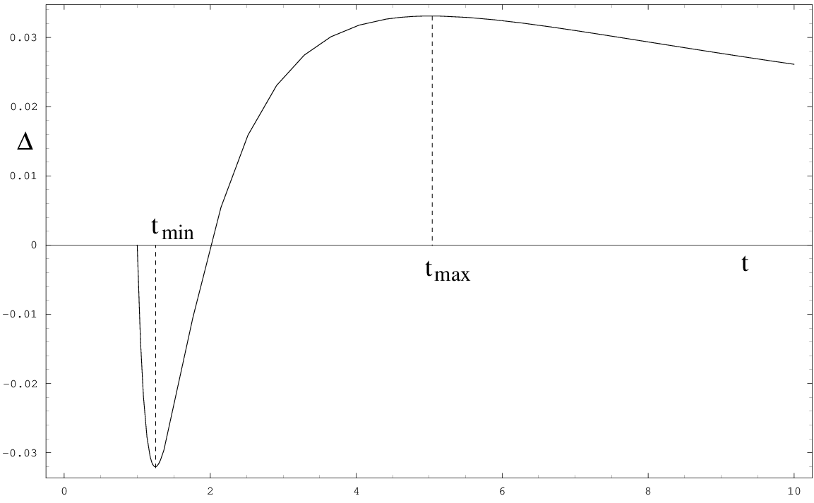
In FIG.1 we have shown the major axes, AC and PR, for and its dual parameter . The corresponding minor axes are QS and AC respectively. In general, the ratio, , of the major axis to the minor axis (for example AC/QS) for is . The ratio, , of the major axis to the minor axis for (for example PR/AC) is . Now it is easy to see that the above two ratios are same, i.e. , if and satisfy the duality relation (37). also measures the scale (the ratio of two major (or minor) axes, i.e. PR/AC (= AC/QS)) through which the supercircle is inflated under the duality transformation (37). In case of exact duality the area should scale by , i.e. . In FIG.7 we have plotted against to see whether such a scaling law gives a good estimate of the area for the dual figure. The maximum aberration from the scaling law is seen to take place at two points viz. and and it is obvious that and satisfy the duality relation (37). The deviation is zero at and thereby vindicating our previous assertion that these 2 cases exhibit exact duality. For the other cases the deviation is very small (within ) and by virtue of that we can safely exploit the duality relation for extracting the eigenvalues in the domain once the results are known for .
V THE semi-empirical formula for supercircular boundary
In this section we propose a semi-empirical formula for determining the eigenspectrum for the case of the supercircular boundary for both type of boundary conditions. In the following we shall consider the Dirichlet and the Neumann boundary conditions separately. The case of the Dirichlet condition is discussed in detail. The Neumann condition can be similarly treated and hence only briefly dwelt upon.
V.1 Dirichlet boundary condition
Given a supercircle of area we consider a square of length and a circle of radius and each having an area . The length of each side of the ‘equal area’ square is,
| (40) |
and the radius of the ‘equal area’ circle is,
| (41) |
The solution to (1), when the boundary is a square () of side is,
| (42a) | |||
| and hence the eigenvalue, | |||
| (42b) | |||
where and are positive integers. It is then easy to see that on (i.e. on , , and ). When the boundary is a circle () of radius , the solution is,
| (43a) | |||
| with and | |||
| (43b) | |||
where is the zero of the order Bessel function, . Now to build up a semi-empirical formula for the case of a supercircle we will attempt to find an expression for the eigenvalue in the range . Further, the duality discussed in the preceding section will allow us to extend our results to making the whole domain as . It is easy to figure out from FIG.1 that in the range the boundary has a shape which is an intermediate between a circle and a square. So it makes sense to try an expression of the form,
| (44) |
i.e. we take an average of and with suitable weight factors. We note that all the eigenvalues are calculated for boundaries enclosing an equal area given by (36). Hence the and the in the equation (42b) and (43b) are identified with the ones appearing in the equation (40) and (41) respectively. To find an explicit form of we note that in the limiting cases and the semi-empirical formula must reduce to,
| (45) |
In other words, in such limits, we must have,
| (46) |
Clearly, there can be infinitely many choices of fulfilling the above criteria (46). The simplest choice is . Unfortunately the eigenvalues calculated with this choice does not match very well with the corresponding numerical results. So an exact form of these weight factors cannot be found out from the above arguments only and is best obtained through a ‘trial and error’ method. We have explored different choices of , calculating the eigenvalues and comparing them with the numerical results. As the next plausible candidate we take and try to estimate the best using numerical results. Finally we have settled for the choice, , so that
| (47) |
So the final expression for the eigenvalue for a supercircle with an exponent is furnished through the following expression:
| (48) |
where and are the eigenvalues for a unit area square and a unit area circle respectively. For a particular excited mode and have to be chosen properly. In Table 1 we have shown the exact mapping between the parameters and of and of for the first 10 states. The eigenvalues (including the degeneracies) and are arranged in increasing order of magnitude and are then matched one to one. Note that all the states with for the circle are doubly degenerate and hence are written twice. Each pair of and corresponds to one . Here we have excluded the trivial case and Having done this we next embark upon the task of finding the eigenvalues in the regime . To find an explicit form of in this region we note that in the limiting cases and the semi-empirical formula should yield,
| (49) |
i.e. we require,
| (50) |
This is where the duality relation (37) comes into play. Plugging it in (47) we arrive at the following functional form of ,
| (51) |
Clearly, such a choice of satisfies the limiting conditions. So, finally for lying in the range the duality implies that the expression for the eigenvalues will be:
| (52) |
Using the above expressions we have evaluated the eigenvalues for the first 21 states (including the degenerate ones) for a supercircle and compared them with the numerically obtained values. The comparisons are shown in FIG.8, FIG.9 and FIG.10. We find that the agreement is excellent over a wide range of the supercircular exponent except for a few cases which we discuss in the next section.
V.2 Neumann boundary condition
In case of the Neumann boundary condition we must have on . The vanishing of the normal derivative implies that for the square boundary with side the eigenfunction should now be,
| (53) |
This, however, has no effect on the eigenvalues with the exception of , and , for which one now has non trivial . On the other hand, for the circular boundary of radius the eigenfunction remains the same as before, but the Neumann boundary condition dictates that we must have,
| (54) |
where is now the zero of the derivative of the order Bessel function, i.e. . Barring these slight modifications, the basic recipe for finding out the eigenvalues remains unaltered from the Dirichlet case. The eigenvalues are given by the expressions (48) and (52) with properly matched and . In Table 2 we have illustrated the exact matching between the parameters by considering some low lying modes. Here also we have excluded the trivial case and as it was done for the Dirichlet case. We have plotted the eigenvalues for the first 18 states (including the degenerate ones) and compared them with the numerical results in FIG.11 and FIG.12. Once again the matching is found to be reasonably good save and except a few levels whose discussion we postpone to the next section. Comparison of the empirical and the numerical eigenvalues for the first seven states for a supercircle with exponent for both type of boundary conditions is given in Table 3.
VI CONCLUSION
In this paper we have generalised the formalism developed in [3] to encompass the case of Neumann type boundary condition. We have also explicitly verified the results for two boundary geometries - supercircle and ellipse. This is quite significant since the Helmholtz equation is not exactly solvable for such geometries. Here we briefly highlight the salient features which make our formalism different from the existing ones. The scheme we develop is completely different from those prevalent to attack such kind of boundary value problems. However, it does have a parallel in the Rayleigh-Schrödinger type potential perturbation in quantum mechanics. In fact, one of the primary motivations of the order by order construction of the Fourier series in [3] was to make contact with the time independent perturbation theory in quantum mechanics. In 2-level systems in quantum mechanics one witnesses the phenomena of level crossing when the Hamiltonian is perturbed. This is most easily achieved by placing the system in a constant electric or magnetic field [43]. The analogy with quantum mechanics is further consolidated with the observation that boundary perturbation can also induce crossing of the levels. Although in quantum mechanics one usually solves a Dirichlet boundary value problem, here we show that the phenomena of level crossing can appear even in Neumann type problems. Another unique feature is that unlike any other perturbation scheme ours does not require a separate formalism to treat degeneracies. Degenerate states are handled equally elegantly as the non-degenerate ones. As opposed to earlier schemes where the perturbation parameter is an artificial one here a real one, extracted from the parameters defining the irregular boundary, serves as a perturbation parameter. It is found that for any perturbation the higher states are more affected. We have plotted beyond the 20th excited level and have shown that the analytical perturbation procedure developed here does reasonably well even for such higher states. Finally, our scheme is a one shot process. If there is an equation for the family of closed curves (like that in an ellipse or a supercircle) one can have the full spectrum just from a knowledge of the parameters of the equation. We exploit the parameters of curve equation as the perturbation parameter which is a measure of the deviation from a circle and obtain the results in one go. One has to just substitute the parameter values to get the new spectrum whereas in all other existing schemes one has to find each time the Fourier coefficients and then substitute even if the curve is of the same family.
Besides the phenomenon of level crossing, another interesting case is when the levels just manage to evade a crossing and veers off after touching each other tangentially. For the 2-level quantum mechanical system mentioned here one can in fact set up a criteria to predict whether or not a pair of levels will cross. It will be interesting to explore the possibility of formulating an analogous criteria for boundary perturbation. A closely related problem is to investigate why the perturbation theory falters whenever the levels display repulsion for elliptical boundary. We have seen that for the elliptical boundary, the agreement between the analytical and numerical results is quite outstanding for small values of . The only blemish is the inability of the scheme to predict the level repulsions. A proper understanding of this level repulsion can be a potential topic for further study.
We have also put forward a single parameter semi-empirical formula giving the eigenspectrum of the 2 dimensional homogeneous Helmholtz equation with Dirichlet or Neumann condition on a supercircular boundary. It is found that the prescription gives results to a high degree of accuracy for a wide range of the parameter for both type of boundary conditions barring a few cases. In fact we have checked explicitly for and the agreement is rather impressive throughout the range. This is quite remarkable considering the fact that a semi-empirical formula involving just a single parameter, the supercircular exponent , yields such accurate results. This assumes more significance because the problem is not exactly solvable analytically. Even the perturbative scheme that we have developed works only for small deformations about the circle. On the other hand, the semi empirical formula, supplemented with the duality relation gives us an analytic handle to extract the eigenvalues even when . A possible generalisation would be to attempt a similar formula when , i.e. we have a concave curve. We would also like to point out a very peculiar feature that has plagued the semi-empirical results: the abnormal behaviour of the Bessel function . The semi-empirical formula for the Dirichlet boundary condition does not provide the anticipated results whenever there is a contribution to from the zeros of which is quite mysterious indeed. The first such case arises from which contributes to the eigenvalues of the second and the third modes. It is clear from Table 3 that for the Dirichlet case the agreement between the empirical and the numerical values is outstanding and the maximum error is except for the second and the third states where the error is within . The next victims are the ninth and the tenth modes which receive contribution from the second zero of and in both cases the degree of mismatch is little pronounced but the relative errors are within . In the case of the Neumann condition also there is disparity between the numerical and the semiempirical predictions for some of the eigenvalues. The first instance occurs in the case of the first and the second modes both of which involve a contribution from . Table 3 also shows that the errors for the aforesaid modes are around for . For the other modes the matching is very good and the errors are within . The next levels afflicted with this anomaly are the eleventh and the twelfth ones which involve . This mysterious behaviour of is something which cannot be accounted for at this point and calls for deeper study. Strangely enough, all these states also involve level repulsion. In this context, it may be mentioned that Chakraborty et al [3] had earlier reported the failure of perturbative treatment in the cases where the levels repel each other for the case of Dirichlet condition on an elliptical boundary and there also the levels were associated with . Here too the analytical scheme for the Neumann boundary on the supercircle reveals that the states display level repulsion. From the results at hand it seems as if level repulsion and abnormality go hand in hand. But we do not know whether this is sheer coincidence or there is an underlying connection between the two. In any case we think it would be worthwhile to look into this aspect.
VII Acknowledgments
SP would like to acknowledge Council of Scientific and Industrial Research (CSIR), India for providing the financial support.
References
- [1] I. Sobchenko, J. Pesicka, D.Baither, R. Reichelt, E. Nembach, Applied Physics Letters 89, 133107 (2006).
- [2] N. Bera, J.K. Bhattacharjee, S. Mitra, S.P. Khastgir, Eur. Phys. J. D 46, 41 (2008).
- [3] S. Chakraborty, J.K. Bhattacharjee, S.P. Khastgir, J. Phys. A: Math. Gen. 42, 195301 (2009).
- [4] K. Lis, S. Bednarek, B. Szafran, J. Adamowski, Physica E 17, 494 (2003).
- [5] P.S. Drouvelis, P. Schmelcher, F.K. Diakonos, Physical Review B 69, 155312 (2004).
- [6] I. Magnúsdóttir, V. Gudmundsson, Physical Review B 60, 16591 (1999).
- [7] M. Kac, American Mathematical Monthly 73, 1-23 (1966).
- [8] C. Gordon, D. Webb, S. Wolpert, Inventiones Mathematicae 110, 1 (1992).
- [9] E. Doron, U. Smilansky, Nonlinearity 5, 1055 (1992).
- [10] B. Dietz, U. Smilansky, CHAOS 3, 581 (1993).
- [11] M.V. Berry, J. Phys. A: Math. Gen. 27, L391 (1994).
- [12] J.P. Eckmann, C.A. Pillet, Commun. Math. Phys. 170, 283 (1995).
- [13] S. Tasaki, T. Harayama, A. Shudo, Phys. Rev. E 56, R13 (1997).
- [14] Y. Okada, A. Shudo, S. Tasaki, T. Harayama, J. Phys. A: Math. Gen. 38, L163 (2005).
- [15] H.R. Krishnamurthy, H.S. Mani, H.C. Verma, J. Phys. A: Math. Gen. 15, 2131 (1982).
- [16] J. Mazumdar, Shock and Vibration Digest 7, 75 (1975).
- [17] J. Mazumdar, Shock and Vibration Digest 11, 25 (1979).
- [18] J. Mazumdar, Shock and Vibration Digest 14, 11 (1982).
- [19] J.R. Kuttler, V.G. Sigillito, SIAM Review 26, 163 (1984).
- [20] P. Amore, J. Phys. A: Math. Theor. 41, 265206 (2008).
- [21] P. Amore, J. Math. Phys. 51, 052105 (2010).
- [22] R.C.T. George, P.R. Shaw, J. Acoust. Soc. Am. 56, 796 (1974).
- [23] H.B. Wilson, R.W. Scharstein, Journal of Engineering Mathematics 57, 1 41 (2007).
- [24] R. Hettich, E. Haaren, M. Ries, G. Still, Journal of Applied Mathematics and Mechanics 67, 12 589 (1987).
- [25] B.A. Troesch, H.R. Troesch, Mathematics of Computation 27, 24 (1973).
- [26] D.L. Kaufman, I. Kosztin, K. Schulten, Am. J. Phys. 67, 133 (1998).
- [27] E. Vergini, M. Saraceno, Physical Review B 52, 2204 (1995).
- [28] D. Cohen, N. Lepore, E.J. Heller, J. Phys. A: Math. Theor. 37, 2139 (2004).
- [29] I. Kosztin, K. Schulten, Int. J. Mod. Phys. C 8, 233 (1997).
- [30] M. Robnik, J. Phys. A: Math. Theor. 17, 1049 (1984).
- [31] E. Lijnen, L.F. Chibotaru, A. Ceulemans, Physical Review B 77, 016702 (2008).
- [32] J.W.S.B. Rayleigh, Theory of Sound, 2nd. ed., (Dover, New York, 1945).
- [33] A.L. Fetter, J.D. Walecka, Theoretical Mechanics of Particles and Continua, (McGraw Hill Book Company, 1980).
- [34] P.M. Morse, H. Feshbach, Methods of Theoretical Physics, (Vol.2, McGraw Hill Book Company, 1983).
- [35] R.G. Parker, C.D. Mote Jr., Journal of Sound and Vibration 211, 3 389 (1998).
- [36] A.H. Nayfeh, Introduction to Perturbation Techniques, (J. Wiley, New York, 1981).
- [37] W.W. Read, Mathematical and Computer Modelling 24, 2 23 (1996).
- [38] Y. Wu, P.N. Shivakumar, Computers and Mathematics with Applications 55, 6 1129 (2008).
- [39] L. Molinari, J. Phys. A. Math. Gen. 30, 6517 (1997).
- [40] R. Dubertrand, E. Bogomolny, N. Djellali, M. Lebental, C. Schmit, Physical Review A 77, 013804 (2008).
- [41] M. Gardner, Piet Hein’s Superellipse, Ch. 18 in Mathematical Carnival: A new Round-Up of Tantalizers and Puzzles from Scientific American., (New York: Vintage, pp. 240-254, 1977).
- [42] N.T. Gridgeman, Lamé Ovals, Math. Gaz. 54, 31 (1970).
- [43] K. Gottfried, T. Yan, Quantum Mechanics: Fundamentals, 2nd ed. (Springer, 2003).
| State | |||||||
| = | |||||||
| 1 | 1 | 2 | Ground | 0 | 1 | 2.40483 | 5.7832 |
| 1 | 2 | 5 | 1 | 2 | 3.83171 | 14.6820 | |
| 2 | 1 | 5 | 1 | 2 | 3.83171 | 14.6820 | |
| 2 | 2 | 8 | 2 | 1 | 5.13562 | 26.3746 | |
| 1 | 3 | 10 | 2 | 1 | 5.13562 | 26.3746 | |
| 3 | 1 | 10 | 0 | 2 | 5.52008 | 30.4713 | |
| 2 | 3 | 13 | 3 | 1 | 6.38016 | 40.7064 | |
| 3 | 2 | 13 | 3 | 1 | 6.38016 | 40.7064 | |
| 1 | 4 | 17 | 1 | 3 | 7.01559 | 49.2185 | |
| 4 | 1 | 17 | 1 | 3 | 7.01559 | 49.2185 |
| State | |||||||
| = | |||||||
| 0 | 1 | 1 | Ground | 1 | 1 | 1.8412 | 3.3900 |
| 1 | 0 | 1 | 1 | 1 | 1.8412 | 3.3900 | |
| 1 | 1 | 2 | 2 | 1 | 3.0542 | 9.3281 | |
| 0 | 2 | 4 | 2 | 1 | 3.0542 | 9.3281 | |
| 2 | 0 | 4 | 0 | 2 | 3.8317 | 14.6819 | |
| 1 | 2 | 5 | 3 | 1 | 4.2012 | 17.6501 | |
| 2 | 1 | 5 | 3 | 1 | 4.2012 | 17.6501 | |
| 2 | 2 | 8 | 4 | 1 | 5.3175 | 28.2758 | |
| 0 | 3 | 9 | 4 | 1 | 5.3175 | 28.2758 |
| State | Dirichlet condition | Neumann condition | ||||
| Degeneracy | Empirical | Numerical | Degeneracy | Empirical | Numerical | |
| Ground | 1 | 6.7077 | 6.7178 | 2 | 3.8542 | 3.8477 |
| First | 2 | 16.9942 | 16.9954 | 1 | 10.2669 | 9.3361 |
| Second | 1 | 30.0858 | 29.0001 | 1 | 11.1682 | 12.1291 |
| Third | 1 | 30.9870 | 32.0603 | 1 | 16.5436 | 16.5417 |
| Fourth | 1 | 35.1002 | 35.0087 | 2 | 19.9743 | 20.0064 |
| Fifth | 2 | 46.7285 | 46.4754 | 1 | 31.9947 | 31.4117 |
| Sixth | 2 | 57.0773 | 57.1111 | 1 | 32.4453 | 32.6240 |