Relative Density-Ratio Estimation
for Robust Distribution Comparison
Abstract
Divergence estimators based on direct approximation of density-ratios without going through separate approximation of numerator and denominator densities have been successfully applied to machine learning tasks that involve distribution comparison such as outlier detection, transfer learning, and two-sample homogeneity test. However, since density-ratio functions often possess high fluctuation, divergence estimation is still a challenging task in practice. In this paper, we propose to use relative divergences for distribution comparison, which involves approximation of relative density-ratios. Since relative density-ratios are always smoother than corresponding ordinary density-ratios, our proposed method is favorable in terms of the non-parametric convergence speed. Furthermore, we show that the proposed divergence estimator has asymptotic variance independent of the model complexity under a parametric setup, implying that the proposed estimator hardly overfits even with complex models. Through experiments, we demonstrate the usefulness of the proposed approach.
keywords
Density ratio, Pearson divergence, Outlier detection, Two-sample homogeneity test, Unconstrained least-squares importance fitting.1 Introduction
Comparing probability distributions is a fundamental task in statistical data processing. It can be used for, e.g., outlier detection (Smola et al., 2009; Hido et al., 2011), two-sample homogeneity test (Gretton et al., 2007; Sugiyama et al., 2011), and transfer learning (Shimodaira, 2000; Sugiyama et al., 2007).
A standard approach to comparing probability densities and would be to estimate a divergence from to , such as the Kullback-Leibler (KL) divergence (Kullback and Leibler, 1951):
A naive way to estimate the KL divergence is to separately approximate the densities and from data and plug the estimated densities in the above definition. However, since density estimation is known to be a hard task (Vapnik, 1998), this approach does not work well unless a good parametric model is available. Recently, a divergence estimation approach which directly approximates the density ratio,
without going through separate approximation of densities and has been proposed (Sugiyama et al., 2008; Nguyen et al., 2010). Such density-ratio approximation methods were proved to achieve the optimal non-parametric convergence rate in the mini-max sense.
However, the KL divergence estimation via density-ratio approximation is computationally rather expensive due to the non-linearity introduced by the ‘log’ term. To cope with this problem, another divergence called the Pearson (PE) divergence (Pearson, 1900) is useful. The PE divergence from to is defined as
The PE divergence is a squared-loss variant of the KL divergence, and they both belong to the class of the Ali-Silvey-Csiszár divergences (Ali and Silvey, 1966; Csiszár, 1967, which is also known as the -divergences, see). Thus, the PE and KL divergences share similar properties, e.g., they are non-negative and vanish if and only if .
Similarly to the KL divergence estimation, the PE divergence can also be accurately estimated based on density-ratio approximation (Kanamori et al., 2009): the density-ratio approximator called unconstrained least-squares importance fitting (uLSIF) gives the PE divergence estimator analytically, which can be computed just by solving a system of linear equations. The practical usefulness of the uLSIF-based PE divergence estimator was demonstrated in various applications such as outlier detection (Hido et al., 2011), two-sample homogeneity test (Sugiyama et al., 2011), and dimensionality reduction (Suzuki and Sugiyama, 2010).
In this paper, we first establish the non-parametric convergence rate of the uLSIF-based PE divergence estimator, which elucidates its superior theoretical properties. However, it also reveals that its convergence rate is actually governed by the ‘sup’-norm of the true density-ratio function: . This implies that, in the region where the denominator density takes small values, the density ratio tends to take large values and therefore the overall convergence speed becomes slow. More critically, density ratios can even diverge to infinity under a rather simple setting, e.g., when the ratio of two Gaussian functions is considered (Cortes et al., 2010). This makes the paradigm of divergence estimation based on density-ratio approximation unreliable.
In order to overcome this fundamental problem, we propose an alternative approach to distribution comparison called -relative divergence estimation. In the proposed approach, we estimate the quantity called the -relative divergence, which is the divergence from to the -mixture density for . For example, the -relative PE divergence is given by
We estimate the -relative divergence by direct approximation of the -relative density-ratio:
A notable advantage of this approach is that the -relative density-ratio is always bounded above by when , even when the ordinary density-ratio is unbounded. Based on this feature, we theoretically show that the -relative PE divergence estimator based on -relative density-ratio approximation is more favorable than the ordinary density-ratio approach in terms of the non-parametric convergence speed.
We further prove that, under a correctly-specified parametric setup, the asymptotic variance of our -relative PE divergence estimator does not depend on the model complexity. This means that the proposed -relative PE divergence estimator hardly overfits even with complex models.
Through extensive experiments on outlier detection, two-sample homogeneity test, and transfer learning, we demonstrate that our proposed -relative PE divergence estimator compares favorably with alternative approaches.
The rest of this paper is structured as follows. In Section 2, our proposed relative PE divergence estimator is described. In Section 3, we provide non-parametric analysis of the convergence rate and parametric analysis of the variance of the proposed PE divergence estimator. In Section 4, we experimentally evaluate the performance of the proposed method on various tasks. Finally, in Section 5, we conclude the paper by summarizing our contributions and describing future prospects.
2 Estimation of Relative Pearson Divergence via Least-Squares Relative Density-Ratio Approximation
In this section, we propose an estimator of the relative Pearson (PE) divergence based on least-squares relative density-ratio approximation.
2.1 Problem Formulation
Suppose we are given independent and identically distributed (i.i.d.) samples from a -dimensional distribution with density and i.i.d. samples from another -dimensional distribution with density :
The goal of this paper is to compare the two underlying distributions and only using the two sets of samples and .
For , let be the -mixture density of and :
Let be the -relative density-ratio of and :
| (1) |
We define the -relative PE divergence from to as
| (2) |
where denotes the expectation of under :
When , is reduced to the ordinary PE divergence. Thus, the -relative PE divergence can be regarded as a ‘smoothed’ extension of the ordinary PE divergence.
Below, we give a method for estimating the -relative PE divergence based on the approximation of the -relative density-ratio.
2.2 Direct Approximation of -Relative Density-Ratios
Here, we describe a method for approximating the -relative density-ratio (1).
Let us model the -relative density-ratio by the following kernel model:
where are parameters to be learned from data samples, ⊤ denotes the transpose of a matrix or a vector, and is a kernel basis function. In the experiments, we use the Gaussian kernel:
where () is the kernel width.
The parameters in the model are determined so that the following expected squared-error is minimized:
where we used in the third term. Approximating the expectations by empirical averages, we obtain the following optimization problem:
| (3) |
where a penalty term is included for regularization purposes, and denotes the regularization parameter. is the matrix with the -th element
| (4) |
is the -dimensional vector with the -th element
It is easy to confirm that the solution of Eq.(3) can be analytically obtained as
where denotes the -dimensional identity matrix. Finally, a density-ratio estimator is given as
| (5) |
When , the above method is reduced to a direct density-ratio estimator called unconstrained least-squares importance fitting (Kanamori et al., 2009, uLSIF;). Thus, the above method can be regarded as an extension of uLSIF to the -relative density-ratio. For this reason, we refer to our method as relative uLSIF (RuLSIF).
The performance of RuLSIF depends on the choice of the kernel function (the kernel width in the case of the Gaussian kernel) and the regularization parameter . Model selection of RuLSIF is possible based on cross-validation with respect to the squared-error criterion , in the same way as the original uLSIF (Kanamori et al., 2009).
A MATLAB implementation of RuLSIF is available from
(made public after acceptance)
2.3 -Relative PE Divergence Estimation Based on RuLSIF
Using an estimator of the -relative density-ratio , we can construct estimators of the -relative PE divergence (2). After a few lines of calculation, we can show that the -relative PE divergence (2) is equivalently expressed as
Note that the first line can also be obtained via Legendre-Fenchel convex duality of the divergence functional (Rockafellar, 1970).
Based on these expressions, we consider the following two estimators:
| (6) | ||||
| (7) |
We note that the -relative PE divergence (2) can have further different expressions than the above ones, and corresponding estimators can also be constructed similarly. However, the above two expressions will be particularly useful: the first estimator has superior theoretical properties (see Section 3) and the second one is simple to compute.
2.4 Illustrative Examples
Here, we numerically illustrate the behavior of RuLSIF (5) using toy datasets. Let the numerator distribution be , where denotes the normal distribution with mean and variance . The denominator distribution is set as follows:
- (a)
-
: and are the same.
- (b)
-
: has smaller standard deviation than .
- (c)
-
: has larger standard deviation than .
- (d)
-
: and have different means.
- (e)
-
: contains an additional component to .
We draw samples from the above densities, and compute RuLSIF for , , and .
 |
 |
 |
 |
 |
 |
 |
 |
 |
 |
 |
 |
 |
 |
 |
 |
 |
 |
 |
 |
Figure 1 shows the true densities, true density-ratios, and their estimates by RuLSIF. As can be seen from the graphs, the profiles of the true -relative density-ratios get smoother as increases. In particular, in the datasets (b) and (d), the true density-ratios for diverge to infinity, while those for and are bounded (by ). Overall, as gets large, the estimation quality of RuLSIF tends to be improved since the complexity of true density-ratio functions is reduced.
Note that, in the dataset (a) where , the true density-ratio does not depend on since for any . However, the estimated density-ratios still depend on through the matrix (see Eq.(4)).
3 Theoretical Analysis
In this section, we analyze theoretical properties of the proposed PE divergence estimators. More specifically, we provide non-parametric analysis of the convergence rate in Section 3.1, and parametric analysis of the estimation variance in Section 3.2. Since our theoretical analysis is highly technical, we focus on explaining practical insights we can gain from the theoretical results here; we describe all the mathematical details of the non-parametric convergence-rate analysis in Appendix A and the parametric variance analysis in Appendix B.
For theoretical analysis, let us consider a rather abstract form of our relative density-ratio estimator described as
| (8) |
where is some function space (i.e., a statistical model) and is some regularization functional.
3.1 Non-Parametric Convergence Analysis
First, we elucidate the non-parametric convergence rate of the proposed PE estimators. Here, we practically regard the function space as an infinite-dimensional reproducing kernel Hilbert space (Aronszajn, 1950, RKHS;) such as the Gaussian kernel space, and as the associated RKHS norm.
3.1.1 Theoretical Results
Let us represent the complexity of the function space by (); the larger is, the more complex the function class is (see Appendix A for its precise definition). We analyze the convergence rate of our PE divergence estimators as tends to infinity for under
The first condition means that tends to zero, but the second condition means that its shrinking speed should not be too fast.
3.1.2 Interpretation
In both Eq.(9) and Eq.(10), the coefficients of the leading terms (i.e., the first terms) of the asymptotic convergence rates become smaller as gets smaller. Since
larger would be more preferable in terms of the asymptotic approximation error. Note that when , can tend to infinity even under a simple setting that the ratio of two Gaussian functions is considered (Cortes et al., 2010, see also the numerical examples in Section 2.4 of this paper). Thus, our proposed approach of estimating the -relative PE divergence (with ) would be more advantageous than the naive approach of estimating the plain PE divergence (which corresponds to ) in terms of the non-parametric convergence rate.
The above results also show that and have different asymptotic convergence rates. The leading term in Eq.(9) is of order , while the leading term in Eq.(10) is of order , which is slightly slower (depending on the complexity ) than . Thus, would be more accurate than in large sample cases. Furthermore, when , holds and thus holds (see Eq.(11)). Then the leading term in Eq.(9) vanishes and therefore has the even faster convergence rate of order , which is slightly slower (depending on the complexity ) than . Similarly, if is close to , and thus holds.
When is not large enough to be able to neglect the terms of , the terms of matter. If and are large (this can happen, e.g., when is close to ), the coefficient of the -term in Eq.(9) can be larger than that in Eq.(10). Then would be more favorable than in terms of the approximation accuracy.
 |
 |
 |
 |
 |
 |
 |
 |
 |
 |
 |
 |
 |
 |
 |
 |
 |
 |
 |
 |
3.1.3 Numerical Illustration
Let us numerically investigate the above interpretation using the same artificial dataset as Section 2.4.
Figure 2 shows the mean and standard deviation of and over runs for , , and , as functions of ( in this experiment). The true (which was numerically computed) is also plotted in the graphs. The graphs show that both the estimators and approach the true as the number of samples increases, and the approximation error tends to be smaller if is larger.
When is large, tends to perform slightly better than . On the other hand, when is small and the number of samples is small, slightly compares favorably with . Overall, these numerical results well agree with our theory.
3.2 Parametric Variance Analysis
Next, we analyze the asymptotic variance of the PE divergence estimator (6) under a parametric setup.
3.2.1 Theoretical Results
As the function space in Eq.(8), we consider the following parametric model:
where is a finite number. Here we assume that the above parametric model is correctly specified, i.e., it includes the true relative density-ratio function : there exists such that
Here, we use RuLSIF without regularization, i.e., in Eq.(8).
Let us denote the variance of (6) by , where randomness comes from the draw of samples and . Then, under a standard regularity condition for the asymptotic normality (van der Vaart, 2000, see Section 3 of), can be expressed and upper-bounded as
| (12) | ||||
| (13) |
Let us denote the variance of by . Then, under a standard regularity condition for the asymptotic normality (van der Vaart, 2000, see Section 3 of), the variance of is asymptotically expressed as
| (14) |
where is the gradient vector of with respect to at , i.e.,
The matrix is defined by
3.2.2 Interpretation
Eq.(12) shows that, up to , the variance of depends only on the true relative density-ratio , not on the estimator of . This means that the model complexity does not affect the asymptotic variance. Therefore, overfitting would hardly occur in the estimation of the relative PE divergence even when complex models are used. We note that the above superior property is applicable only to relative PE divergence estimation, not to relative density-ratio estimation. This implies that overfitting occurs in relative density-ratio estimation, but the approximation error cancels out in relative PE divergence estimation.
On the other hand, Eq.(14) shows that the variance of is affected by the model , since the factor depends on the model complexity in general. When the equality
holds, the variances of and are asymptotically the same. However, in general, the use of would be more recommended.
Eq.(13) shows that the variance can be upper-bounded by the quantity depending on , which is monotonically lowered if is reduced. Since monotonically decreases as increases, our proposed approach of estimating the -relative PE divergence (with ) would be more advantageous than the naive approach of estimating the plain PE divergence (which corresponds to ) in terms of the parametric asymptotic variance.
 |
 |
| with | with |
 |
 |
| with | with |
 |
 |
| with | with |
 |
 |
| with | with |
3.2.3 Numerical Illustration
Here, we show some numerical results for illustrating the above theoretical results using the one-dimensional datasets (b) and (c) in Section 2.4. Let us define the parametric model as
| (15) |
The dimension of the model is equal to . The -relative density-ratio can be expressed using the ordinary density-ratio as
Thus, when , the above model includes the true relative density-ratio of the datasets (b) and (c). We test RuLSIF with and for the model (15) with degree . The parameter is learned so that Eq.(8) is minimized by a quasi-Newton method.
The standard deviations of and for the datasets (b) and (c) are depicted in Figure 4 and Figure 4, respectively. The graphs show that the degree of models does not significantly affect the standard deviation of (i.e., no overfitting), as long as the model includes the true relative density-ratio (i.e., ). On the other hand, bigger models tend to produce larger standard deviations in . Thus, the standard deviation of more strongly depends on the model complexity.
4 Experiments
In this section, we experimentally evaluate the performance of the proposed method in two-sample homogeneity test, outlier detection, and transfer learning tasks.
4.1 Two-Sample Homogeneity Test
First, we apply the proposed divergence estimator to two-sample homogeneity test.
4.1.1 Divergence-Based Two-Sample Homogeneity Test
Given two sets of samples and , the goal of the two-sample homogeneity test is to test the null hypothesis that the probability distributions and are the same against its complementary alternative (i.e., the distributions are different).
By using an estimator of some divergence between the two distributions and , homogeneity of two distributions can be tested based on the permutation test procedure (Efron and Tibshirani, 1993) as follows:
- •
Obtain a divergence estimate using the original datasets and .
- •
Randomly permute the samples, and assign the first samples to a set and the remaining samples to another set .
- •
Obtain a divergence estimate using the randomly shuffled datasets and (note that, since and can be regarded as being drawn from the same distribution, tends to be close to zero).
- •
Repeat this random shuffling procedure many times, and construct the empirical distribution of under the null hypothesis that the two distributions are the same.
- •
Approximate the p-value by evaluating the relative ranking of the original in the distribution of .
When an asymmetric divergence such as the KL divergence (Kullback and Leibler, 1951) or the PE divergence (Pearson, 1900) is adopted for two-sample homogeneity test, the test results depend on the choice of directions: a divergence from to or from to . Sugiyama et al. (2011) proposed to choose the direction that gives a smaller p-value—it was experimentally shown that, when the uLSIF-based PE divergence estimator is used for the two-sample homogeneity test (which is called the least-squares two-sample homogeneity test; LSTT), the heuristic of choosing the direction with a smaller p-value contributes to reducing the type-II error (the probability of accepting incorrect null-hypotheses, i.e., two distributions are judged to be the same when they are actually different), while the increase of the type-I error (the probability of rejecting correct null-hypotheses, i.e., two distributions are judged to be different when they are actually the same) is kept moderate.
Below, we refer to LSTT with as the plain LSTT, LSTT with as the reciprocal LSTT, and LSTT with heuristically choosing the one with a smaller p-value as the adaptive LSTT.
|
 |
 |
 |
|
 |
 |
 |
|
 |
 |
 |
|
 |
 |
 |
4.1.2 Artificial Datasets
We illustrate how the proposed method behaves in two-sample homogeneity test scenarios using the artificial datasets (a)–(d) described in Section 2.4. We test the plain LSTT, reciprocal LSTT, and adaptive LSTT for , , and , with significance level .
The experimental results are shown in Figure 5. For the dataset (a) where (i.e., the null hypothesis is correct), the plain LSTT and reciprocal LSTT correctly accept the null hypothesis with probability approximately . This means that the type-I error is properly controlled in these methods. On the other hand, the adaptive LSTT tends to give slightly lower acceptance rates than for this toy dataset, but the adaptive LSTT with still works reasonably well. This implies that the heuristic of choosing the method with a smaller p-value does not have critical influence on the type-I error.
In the datasets (b), (c), and (d), is different from (i.e., the null hypothesis is not correct), and thus we want to reduce the acceptance rate of the incorrect null-hypothesis as much as possible. In the plain setup for the dataset (b) and the reciprocal setup for the dataset (c), the true density-ratio functions with diverge to infinity, and thus larger makes the density-ratio approximation more reliable. However, does not work well because it produces an overly-smoothed density-ratio function and thus it is hard to be distinguished from the completely constant density-ratio function (which corresponds to ). On the other hand, in the reciprocal setup for the dataset (b) and the plain setup for the dataset (c), small performs poorly since density-ratio functions with large can be more accurately approximated than those with small (see Figure 1). In the adaptive setup, large tends to perform slightly better than small for the datasets (b) and (c).
In the dataset (d), the true density-ratio function with diverges to infinity for both the plain and reciprocal setups. In this case, middle performs the best, which well balances the trade-off between high distinguishability from the completely constant density-ratio function (which corresponds to ) and easy approximability. The same tendency that middle works well can also be mildly observed in the adaptive LSTT for the dataset (d).
Overall, if the plain LSTT (or the reciprocal LSTT) is used, small (or large ) sometimes works excellently. However, it performs poorly in other cases and thus the performance is unstable depending on the true distributions. The plain LSTT (or the reciprocal LSTT) with middle tends to perform reasonably well for all datasets. On the other hand, the adaptive LSTT was shown to nicely overcome the above instability problem when is small or large. However, when is set to be a middle value, the plain LSTT and the reciprocal LSTT both give similar results and thus the adaptive LSTT provides only a small amount of improvement.
Our empirical finding is that, if we have prior knowledge that one distribution has a wider support than the other distribution, assigning the distribution with a wider support to and setting to be a large value seem to work well. If there is no knowledge on the true distributions or two distributions have less overlapped supports, using middle in the adaptive setup seems to be a reasonable choice.
We will systematically investigate this issue using more complex datasets below.
| Datasets | MMD | LSTT | LSTT | LSTT | ||||||
|---|---|---|---|---|---|---|---|---|---|---|
| ( = 0.0) | ( = 0.5) | ( = 0.95) | ||||||||
| banana | 2 | 100 | 0.98 | (0.14) | 0.93 | (0.26) | 0.92 | (0.27) | 0.92 | (0.27) |
| thyroid | 5 | 19 | 0.98 | (0.14) | 0.95 | (0.22) | 0.95 | (0.22) | 0.88 | (0.33) |
| titanic | 5 | 21 | 0.92 | (0.27) | 0.86 | (0.35) | 0.92 | (0.27) | 0.89 | (0.31) |
| diabetes | 8 | 85 | 0.95 | (0.22) | 0.87 | (0.34) | 0.91 | (0.29) | 0.82 | (0.39) |
| breast-cancer | 9 | 29 | 0.98 | (0.14) | 0.91 | (0.29) | 0.94 | (0.24) | 0.92 | (0.27) |
| flare-solar | 9 | 100 | 0.93 | (0.26) | 0.91 | (0.29) | 0.95 | (0.22) | 0.93 | (0.26) |
| heart | 13 | 38 | 0.96 | (0.20) | 0.85 | (0.36) | 0.91 | (0.29) | 0.93 | (0.26) |
| german | 20 | 100 | 0.93 | (0.26) | 0.91 | (0.29) | 0.92 | (0.27) | 0.89 | (0.31) |
| ringnorm | 20 | 100 | 0.95 | (0.22) | 0.93 | (0.26) | 0.91 | (0.29) | 0.85 | (0.36) |
| waveform | 21 | 66 | 0.93 | (0.26) | 0.92 | (0.27) | 0.93 | (0.26) | 0.88 | (0.33) |
| Datasets | MMD | LSTT | LSTT | LSTT | ||||||
|---|---|---|---|---|---|---|---|---|---|---|
| ( = 0.0) | ( = 0.5) | ( = 0.95) | ||||||||
| banana | 2 | 100 | 0.80 | (0.40) | 0.10 | (0.30) | 0.02 | (0.14) | 0.17 | (0.38) |
| thyroid | 5 | 19 | 0.72 | (0.45) | 0.81 | (0.39) | 0.65 | (0.48) | 0.80 | (0.40) |
| titanic | 5 | 21 | 0.79 | (0.41) | 0.86 | (0.35) | 0.87 | (0.34) | 0.88 | (0.33) |
| diabetes | 8 | 85 | 0.38 | (0.49) | 0.42 | (0.50) | 0.47 | (0.50) | 0.57 | (0.50) |
| breast-cancer | 9 | 29 | 0.91 | (0.29) | 0.75 | (0.44) | 0.80 | (0.40) | 0.79 | (0.41) |
| flare-solar | 9 | 100 | 0.59 | (0.49) | 0.81 | (0.39) | 0.55 | (0.50) | 0.66 | (0.48) |
| heart | 13 | 38 | 0.47 | (0.50) | 0.28 | (0.45) | 0.40 | (0.49) | 0.62 | (0.49) |
| german | 20 | 100 | 0.59 | (0.49) | 0.55 | (0.50) | 0.44 | (0.50) | 0.68 | (0.47) |
| ringnorm | 20 | 100 | 0.00 | (0.00) | 0.00 | (0.00) | 0.00 | (0.00) | 0.02 | (0.14) |
| waveform | 21 | 66 | 0.00 | (0.00) | 0.00 | (0.00) | 0.02 | (0.14) | 0.00 | (0.00) |
4.1.3 Benchmark Datasets
Here, we apply the proposed two-sample homogeneity test to the binary classification datasets taken from the IDA repository (Rätsch et al., 2001).
We test the adaptive LSTT with the RuLSIF-based PE divergence estimator for , , and ; we also test the maximum mean discrepancy (Borgwardt et al., 2006, MMD;), which is a kernel-based two-sample homogeneity test method. The performance of MMD depends on the choice of the Gaussian kernel width. Here, we adopt a version proposed by Sriperumbudur et al. (2009), which automatically optimizes the Gaussian kernel width. The p-values of MMD are computed in the same way as LSTT based on the permutation test procedure.
First, we investigate the rate of accepting the null hypothesis when the null hypothesis is correct (i.e., the two distributions are the same). We split all the positive training samples into two sets and perform two-sample homogeneity test for the two sets of samples. The experimental results are summarized in Table 2, showing that the adaptive LSTT with compares favorably with that with and . LSTT with and MMD are comparable to each other in terms of the type-I error.
Next, we consider the situation where the null hypothesis is not correct (i.e., the two distributions are different). The numerator samples are generated in the same way as above, but a half of denominator samples are replaced with negative training samples. Thus, while the numerator sample set contains only positive training samples, the denominator sample set includes both positive and negative training samples. The experimental results are summarized in Table 2, showing that the adaptive LSTT with again compares favorably with that with and . Furthermore, LSTT with tends to outperform MMD in terms of the type-II error.
Overall, LSTT with is shown to be a useful method for two-sample homogeneity test.
4.2 Inlier-Based Outlier Detection
Next, we apply the proposed method to outlier detection.
4.2.1 Density-Ratio Approach to Inlier-Based Outlier Detection
Let us consider an outlier detection problem of finding irregular samples in a dataset (called an “evaluation dataset”) based on another dataset (called a “model dataset”) that only contains regular samples. Defining the density ratio over the two sets of samples, we can see that the density-ratio values for regular samples are close to one, while those for outliers tend to be significantly deviated from one. Thus, density-ratio values could be used as an index of the degree of outlyingness (Smola et al., 2009; Hido et al., 2011).
Since the evaluation dataset usually has a wider support than the model dataset, we regard the evaluation dataset as samples corresponding to the denominator density , and the model dataset as samples corresponding to the numerator density . Then, outliers tend to have smaller density-ratio values (i.e., close to zero). As such, density-ratio approximators can be used for outlier detection.
When evaluating the performance of outlier detection methods, it is important to take into account both the detection rate (i.e., the amount of true outliers an outlier detection algorithm can find) and the detection accuracy (i.e., the amount of true inliers an outlier detection algorithm misjudges as outliers). Since there is a trade-off between the detection rate and the detection accuracy, we adopt the area under the ROC curve (AUC) as our error metric (Bradley, 1997).
|
|
|
| |||||||||||
|---|---|---|---|---|---|---|---|---|---|---|---|---|---|---|
| 1 | .933 | (.089) | .926 | (.100) | .896 | (.124) | ||||||||
| 5 | .882 | (.099) | .891 | (.091) | .894 | (.086) | ||||||||
| 10 | .842 | (.107) | .850 | (.103) | .859 | (.092) | ||||||||
4.2.2 Artificial Datasets
First, we illustrate how the proposed method behaves in outlier detection scenarios using artificial datasets.
Let
where is the dimensionality of and is the -dimensional vector with all one. Note that this setup is the same as the dataset (e) described in Section 2.4 when . Here, the samples drawn from are regarded as inliers, while the samples drawn from are regarded as outliers. We use samples.
Table 3 describes the AUC values for input dimensionality , , and for RuLSIF with , , and . This shows that, as the input dimensionality increases, the AUC values overall get smaller. Thus, outlier detection becomes more challenging in high-dimensional cases.
The result also shows that RuLSIF with small tends to work well when the input dimensionality is low, and RuLSIF with large works better as the input dimensionality increases. This tendency can be interpreted as follows: If is small, the density-ratio function tends to have sharp ‘hollow’ for outlier points (see the leftmost graph in Figure 2(e)). Thus, as long as the true density-ratio function can be accurately estimated, small would be preferable in outlier detection. When the data dimensionality is low, density-ratio approximation is rather easy and thus small tends to perform well. However, as the data dimensionality increases, density-ratio approximation gets harder, and thus large which produces a smoother density-ratio function is more favorable since such a smoother function can be more easily approximated than a ‘bumpy’ one produced by small .
4.2.3 Real-World Datasets
Next, we evaluate the proposed outlier detection method using various real-world datasets:
- IDA repository:
-
The IDA repository (Rätsch et al., 2001) contains various binary classification tasks. Each dataset consists of positive/negative and training/test samples. We use positive training samples as inliers in the “model” set. In the “evaluation” set, we use at most positive test samples as inliers and the first of negative test samples as outliers. Thus, the positive samples are treated as inliers and the negative samples are treated as outliers.
- Speech dataset:
-
An in-house speech dataset, which contains short utterance samples recorded from male subjects speaking in French with sampling rate kHz. From each utterance sample, we extracted a -dimensional line spectral frequencies vector (Kain and Macon, 1998). We randomly take samples from one class and assign them to the model dataset. Then we randomly take samples from the same class and samples from the other class.
- 20 Newsgroup dataset:
-
The 20-Newsgroups dataset11 1 http://people.csail.mit.edu/jrennie/20Newsgroups/ contains newsgroup documents, which contains the following top-level categories: ‘comp’, ‘rec’, ‘sci’, and ‘talk’. Each document is expressed by a -dimensional bag-of-words vector of term-frequencies. We randomly take samples from the ‘comp’ class and assign them to the model dataset. Then we randomly take samples from the same class and samples from one of the other classes for the evaluation dataset.
- The USPS hand-written digit dataset:
-
The USPS hand-written digit dataset22 2 http://www.gaussianprocess.org/gpml/data/ contains digit images. Each image consists of (= ) pixels and each pixel takes an integer value between and as the intensity level. We regard samples in one class as inliers and samples in other classes as outliers. We randomly take samples from the inlier class and assign them to the model dataset. Then we randomly take samples from the same inlier class and samples from one of the other classes for the evaluation dataset.
We compare the AUC scores of RuLSIF with , , and , and one-class support vector machine (OSVM) with the Gaussian kernel (Schölkopf et al., 2001). We used the LIBSVM implementation of OSVM (Chang and Lin, 2001). The Gaussian width is set to the median distance between samples, which has been shown to be a useful heuristic (Schölkopf et al., 2001). Since there is no systematic method to determine the tuning parameter in OSVM, we report the results for and .
The mean and standard deviation of the AUC scores over runs with random sample choice are summarized in Table 4, showing that RuLSIF overall compares favorably with OSVM. Among the RuLSIF methods, small tends to perform well for low-dimensional datasets, and large tends to work well for high-dimensional datasets. This tendency well agrees with that for the artificial datasets (see Section 4.2.2).
| Datasets |
|
|
|
|
| ||||||||||||||||
|---|---|---|---|---|---|---|---|---|---|---|---|---|---|---|---|---|---|---|---|---|---|
| IDA:banana | 2 | .668 | (.105) | .676 | (.120) | .597 | (.097) | .619 | (.101) | .623 | (.115) | ||||||||||
| IDA:thyroid | 5 | .760 | (.148) | .782 | (.165) | .804 | (.148) | .796 | (.178) | .722 | (.153) | ||||||||||
| IDA:titanic | 5 | .757 | (.205) | .752 | (.191) | .750 | (.182) | .701 | (.184) | .712 | (.185) | ||||||||||
| IDA:diabetes | 8 | .636 | (.099) | .610 | (.090) | .594 | (.105) | .575 | (.105) | .663 | (.112) | ||||||||||
| IDA:b-cancer | 9 | .741 | (.160) | .691 | (.147) | .707 | (.148) | .737 | (.159) | .733 | (.160) | ||||||||||
| IDA:f-solar | 9 | .594 | (.087) | .590 | (.083) | .626 | (.102) | .612 | (.100) | .584 | (.114) | ||||||||||
| IDA:heart | 13 | .714 | (.140) | .694 | (.148) | .748 | (.149) | .769 | (.134) | .726 | (.127) | ||||||||||
| IDA:german | 20 | .612 | (.069) | .604 | (.084) | .605 | (.092) | .597 | (.101) | .605 | (.095) | ||||||||||
| IDA:ringnorm | 20 | .991 | (.012) | .993 | (.007) | .944 | (.091) | .971 | (.062) | .992 | (.010) | ||||||||||
| IDA:waveform | 21 | .812 | (.107) | .843 | (.123) | .879 | (.122) | .875 | (.117) | .885 | (.102) | ||||||||||
| Speech | 50 | .788 | (.068) | .830 | (.060) | .804 | (.101) | .821 | (.076) | .836 | (.083) | ||||||||||
| 20News (‘rec’) | 100 | .598 | (.063) | .593 | (.061) | .628 | (.105) | .614 | (.093) | .767 | (.100) | ||||||||||
| 20News (‘sci’) | 100 | .592 | (.069) | .589 | (.071) | .620 | (.094) | .609 | (.087) | .704 | (.093) | ||||||||||
| 20News (‘talk’) | 100 | .661 | (.084) | .658 | (.084) | .672 | (.117) | .670 | (.102) | .823 | (.078) | ||||||||||
| USPS (1 vs. 2) | 256 | .889 | (.052) | .926 | (.037) | .848 | (.081) | .878 | (.088) | .898 | (.051) | ||||||||||
| USPS (2 vs. 3) | 256 | .823 | (.053) | .835 | (.050) | .803 | (.093) | .818 | (.085) | .879 | (.074) | ||||||||||
| USPS (3 vs. 4) | 256 | .901 | (.044) | .939 | (.031) | .950 | (.056) | .961 | (.041) | .984 | (.016) | ||||||||||
| USPS (4 vs. 5) | 256 | .871 | (.041) | .890 | (.036) | .857 | (.099) | .874 | (.082) | .941 | (.031) | ||||||||||
| USPS (5 vs. 6) | 256 | .825 | (.058) | .859 | (.052) | .863 | (.078) | .867 | (.068) | .901 | (.049) | ||||||||||
| USPS (6 vs. 7) | 256 | .910 | (.034) | .950 | (.025) | .972 | (.038) | .984 | (.018) | .994 | (.010) | ||||||||||
| USPS (7 vs. 8) | 256 | .938 | (.030) | .967 | (.021) | .941 | (.053) | .951 | (.039) | .980 | (.015) | ||||||||||
| USPS (8 vs. 9) | 256 | .721 | (.072) | .728 | (.073) | .721 | (.084) | .728 | (.083) | .761 | (.096) | ||||||||||
| USPS (9 vs. 0) | 256 | .920 | (.037) | .966 | (.023) | .982 | (.048) | .989 | (.022) | .994 | (.011) | ||||||||||
4.3 Transfer Learning
Finally, we apply the proposed method to outlier detection.
4.3.1 Transductive Transfer Learning by Importance Sampling
Let us consider a problem of semi-supervised learning (Chapelle et al., 2006) from labeled training samples and unlabeled test samples . The goal is to predict a test output value for a test input point . Here, we consider the setup where the labeled training samples are drawn i.i.d. from , while the unlabeled test samples are drawn i.i.d. from , which is generally different from ; the (unknown) test sample follows . This setup means that the conditional probability is common to training and test samples, but the marginal densities and are generally different for training and test input points. Such a problem is called transductive transfer learning (Pan and Yang, 2010), domain adaptation (Jiang and Zhai, 2007), or covariate shift (Shimodaira, 2000; Sugiyama and Kawanabe, 2011).
Let be a point-wise loss function that measures a discrepancy between and (at input ). Then the generalization error which we would like to ultimately minimize is defined as
where is a function model. Since the generalization error is inaccessible because the true probability is unknown, empirical-error minimization is often used in practice (Vapnik, 1998):
However, under the covariate shift setup, plain empirical-error minimization is not consistent (i.e., it does not converge to the optimal function) if the model is misspecified (Shimodaira, 2000, i.e., the true function is not included in the model; see). Instead, the following importance-weighted empirical-error minimization is consistent under covariate shift:
where is called the importance (Fishman, 1996) in the context of covariate shift adaptation:
However, since importance-weighted learning is not statistically efficient (i.e., it tends to have larger variance), slightly flattening the importance weights is practically useful for stabilizing the estimator. Shimodaira (2000) proposed to use the exponentially-flattened importance weights as
where is called the exponential flattening parameter. corresponds to plain empirical-error minimization, while corresponds to importance-weighted empirical-error minimization; will give an intermediate estimator that balances the trade-off between statistical efficiency and consistency. The exponential flattening parameter can be optimized by model selection criteria such as the importance-weighted Akaike information criterion for regular models (Shimodaira, 2000), the importance-weighted subspace information criterion for linear models (Sugiyama and Müller, 2005), and importance-weighted cross-validation for arbitrary models (Sugiyama et al., 2007).
One of the potential drawbacks of the above exponential flattering approach is that estimation of (i.e., ) is rather hard, as shown in this paper. Thus, when is estimated poorly, all flattened weights are also unreliable and then covariate shift adaptation does not work well in practice. To cope with this problem, we propose to use relative importance weights alternatively:
where () is the -relative importance weight defined by
Note that, compared with the definition of the -relative density-ratio (1), and are swapped in order to be consistent with exponential flattening. Indeed, the relative importance weights play a similar role to exponentially-flattened importance weights; corresponds to plain empirical-error minimization, while corresponds to importance-weighted empirical-error minimization; will give an intermediate estimator that balances the trade-off between efficiency and consistency. We note that the relative importance weights and exponentially flattened importance weights agree only when and ; for , they are generally different.
A possible advantage of the above relative importance weights is that its estimation for does not depend on that for , unlike exponentially-flattened importance weights. Since -relative importance weights for can be reliably estimated by RuLSIF proposed in this paper, the performance of covariate shift adaptation is expected to be improved. Below, we experimentally investigate this effect.
4.3.2 Artificial Datasets
First, we illustrate how the proposed method behaves in covariate shift adaptation using one-dimensional artificial datasets.
In this experiment, we employ the following kernel regression model:
where is the parameter to be learned and is the Gaussian width. The parameter is learned by relative importance-weighted least-squares (RIW-LS):
or exponentially-flattened importance-weighted least-squares (EIW-LS):
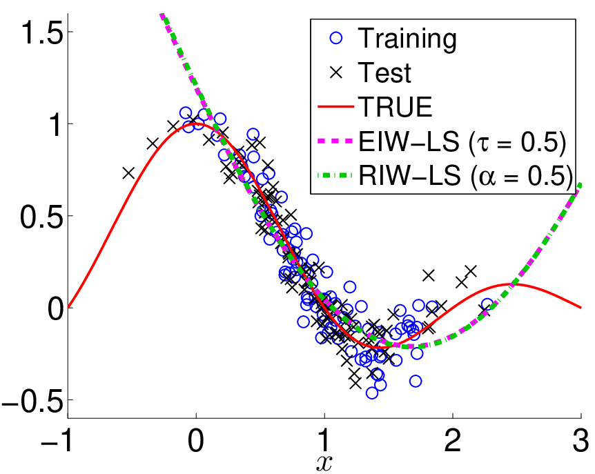
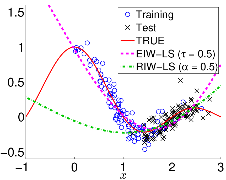
The relative importance weight is estimated by RuLSIF, and the exponentially-flattened importance weight is estimated by uLSIF (i.e., RuLSIF with ). The Gaussian width is chosen by 5-fold importance-weighted cross-validation (Sugiyama et al., 2007).




First, we consider the case where input distributions do not change:
The densities and their ratios are plotted in Figure 6(a). The training output samples are generated as
where is additive noise following . We set and . Figure 6(b) shows a realization of training and test samples as well as learned functions obtained by RIW-LS with and EIW-LS with . This shows that RIW-LS with and EIW-LS with give almost the same functions, and both functions fit the true function well in the test region. Figure 6(c) shows the mean and standard deviation of the test error under the squared loss over runs, as functions of the relative flattening parameter in RIW-LS and the exponential flattening parameter in EIW-LS. The method having a lower mean test error and another method that is comparable according to the t-test at the significance level are specified by ‘’. As can be observed, the proposed RIW-LS compares favorably with EIW-LS.
Next, we consider the situation where input distribution changes (Figure 7(a)):
The output values are created in the same way as the previous case. Figure 7(b) shows a realization of training and test samples as well as learned functions obtained by RIW-LS with and EIW-LS with . This shows that RIW-LS with fits the true function slightly better than EIW-LS with in the test region. Figure 7(c) shows that the proposed RIW-LS tends to outperform EIW-LS, and the standard deviation of the test error for RIW-LS is much smaller than EIW-LS. This is because EIW-LS with is based on an importance estimate with , which tends to have high fluctuation. Overall, the stabilization effect of relative importance estimation was shown to improve the test accuracy.
4.3.3 Real-World Datasets
Finally, we evaluate the proposed transfer learning method on a real-world transfer learning task.

We consider the problem of human activity recognition from accelerometer data collected by iPod touch33 3 http://alkan.mns.kyutech.ac.jp/web/data.html. In the data collection procedure, subjects were asked to perform a specific action such as walking, running, and bicycle riding. The duration of each task was arbitrary and the sampling rate was Hz with small variations. An example of three-axis accelerometer data for “walking” is plotted in Figure 8.
To extract features from the accelerometer data, each data stream was segmented in a sliding window manner with window width seconds and sliding step second. Depending on subjects, the position and orientation of iPod touch was arbitrary—held by hand or kept in a pocket or a bag. For this reason, we decided to take the -norm of the -dimensional acceleration vector at each time step, and computed the following orientation-invariant features from each window: mean, standard deviation, fluctuation of amplitude, average energy, and frequency-domain entropy (Bao and Intille, 2004; Bharatula et al., 2005).
Let us consider a situation where a new user wants to use the activity recognition system. However, since the new user is not willing to label his/her accelerometer data due to troublesomeness, no labeled sample is available for the new user. On the other hand, unlabeled samples for the new user and labeled data obtained from existing users are available. Let labeled training data be the set of labeled accelerometer data for existing users. Each user has at most labeled samples for each action. Let unlabeled test data be unlabeled accelerometer data obtained from the new user.
| Task | KLR | RIW-KLR | EIW-KLR | IW-KLR | ||||
|---|---|---|---|---|---|---|---|---|
| (, ) | () | () | (, ) | |||||
| Walks vs. run | 0.803 | (0.082) | 0.889 | (0.035) | 0.882 | (0.039) | 0.882 | (0.035) |
| Walks vs. bicycle | 0.880 | (0.025) | 0.892 | (0.035) | 0.867 | (0.054) | 0.854 | (0.070) |
| Walks vs. train | 0.985 | (0.017) | 0.992 | (0.008) | 0.989 | (0.011) | 0.983 | (0.021) |
We use kernel logistic regression (KLR) for activity recognition. We compare the following four methods:
- •
Plain KLR without importance weights (i.e., or ).
- •
KLR with relative importance weights for .
- •
KLR with exponentially-flattened importance weights for .
- •
KLR with plain importance weights (i.e., or ).
The experiments are repeated times with different sample choice for and . Table 5 depicts the classification accuracy for three binary-classification tasks: walk vs. run, walk vs. riding a bicycle, and walk vs. taking a train. The classification accuracy is evaluated for samples from the new user that are not used for classifier training (i.e., the test samples are different from unlabeled samples). The table shows that KLR with relative importance weights for compares favorably with other methods in terms of the classification accuracy. KLR with plain importance weights and KLR with exponentially-flattened importance weights for are outperformed by KLR without importance weights in the walk vs. riding a bicycle task due to the instability of importance weight estimation for or .
Overall, the proposed relative density-ratio estimation method was shown to be useful also in transfer learning under covariate shift.
5 Conclusion
In this paper, we proposed to use a relative divergence for robust distribution comparison. We gave a computationally efficient method for estimating the relative Pearson divergence based on direct relative density-ratio approximation. We theoretically elucidated the convergence rate of the proposed divergence estimator under non-parametric setup, which showed that the proposed approach of estimating the relative Pearson divergence is more preferable than the existing approach of estimating the plain Pearson divergence. Furthermore, we proved that the asymptotic variance of the proposed divergence estimator is independent of the model complexity under a correctly-specified parametric setup. Thus, the proposed divergence estimator hardly overfits even with complex models. Experimentally, we demonstrated the practical usefulness of the proposed divergence estimator in two-sample homogeneity test, inlier-based outlier detection, and transductive transfer learning under covariate shift.
In addition to two-sample homogeneity test, outlier detection, and transfer learning, density ratios were shown to be useful for tackling various machine learning problems, including multi-task learning (Bickel et al., 2008; Simm et al., 2011), independence test (Sugiyama and Suzuki, 2011), feature selection (Suzuki et al., 2009), causal inference (Yamada and Sugiyama, 2010), independent component analysis (Suzuki and Sugiyama, 2011), dimensionality reduction (Suzuki and Sugiyama, 2010), unpaired data matching (Yamada and Sugiyama, 2011), clustering (Kimura and Sugiyama, 2011), conditional density estimation (Sugiyama et al., 2010), and probabilistic classification (Sugiyama, 2010). Thus, it would be promising to explore more applications of the proposed relative density-ratio approximator beyond two-sample homogeneity test, outlier detection, and transfer learning tasks.
acknowledgments-disclosure-of-funding.
MY was supported by the JST PRESTO program, TS was partially supported by MEXT KAKENHI 22700289 and Aihara Project, the FIRST program from JSPS, initiated by CSTP, TK was partially supported by Grant-in-Aid for Young Scientists (20700251), HH was supported by the FIRST program, and MS was partially supported by SCAT, AOARD, and the FIRST program.Appendix A Technical Details of Non-Parametric Convergence Analysis
Here, we give the technical details of the non-parametric convergence analysis described in Section 3.1.
A.1 Results
For notational simplicity, we define linear operators as
For , we define and as
We estimate the Pearson divergence between and through estimating the density ratio
Let us consider the following density ratio estimator:
where and is a non-negative regularization functional such that
| (16) |
A possible estimator of the Pearson (PE) divergence is
Another possibility is
A useful example is to use a reproducing kernel Hilbert space (Aronszajn, 1950, RKHS;) as and the RKHS norm as . Suppose is an RKHS associated with bounded kernel :
Let denote the norm in the RKHS . Then satisfies Eq.(16):
where we used the reproducing property of the kernel and Schwartz’s inequality. Note that the Gaussian kernel satisfies this with . It is known that the Gaussian kernel RKHS spans a dense subset in the set of continuous functions. Another example of RKHSs is Sobolev space. The canonical norm for this space is the integral of the squared derivatives of functions. Thus the regularization term imposes the solution to be smooth. The RKHS technique in Sobolev space has been well exploited in the context of spline models (Wahba, 1990). We intend that the regularization term is a generalization of the RKHS norm. Roughly speaking, is like a “norm” of the function space .
We assume that the true density-ratio function is contained in the model and is bounded from above:
Let be a ball of with radius :
To derive the convergence rate of our estimator, we utilize the bracketing entropy that is a complexity measure of a function class (van der Vaart and Wellner, 1996, see p. 83 of).
Definition 1.
Given two functions and , the bracket is the set of all functions with for all . An -bracket with respect to is a bracket with . The bracketing entropy is the logarithm of the minimum number of -brackets with respect to needed to cover a function set .
We assume that there exists such that, for all ,
| (17) |
This quantity represents a complexity of function class —the larger is, the more complex the function class is because, for larger , more brackets are needed to cover the function class. The Gaussian RKHS satisfies this condition for arbitrarily small (Steinwart and Scovel, 2007). Note that when is the RKHS norm, the condition (17) holds for all if that holds for .
Then we have the following theorem.
Theorem 2.
Let , , and . Under the above setting, if and , then we have
and
where denotes the asymptotic order in probability.
In the proof of Theorem 2, we use the following auxiliary lemma.
Lemma 3.
A.2 Proof of Lemma 3
First, we prove Lemma 3.
From the definition, we obtain
On the other hand, indicates
Therefore, to bound , it suffices to bound the left-hand side of the above inequality.
Define and as
To bound , we need to bound the bracketing entropies of . We show that
This can be shown as follows. Let and be a -bracket for with respect to ; and . Without loss of generality, we can assume that . Then and defined as
are also a bracket such that for all s.t. and because and the following relation is met:
Therefore the condition for the bracketing entropies (17) gives . We can also show that in the same fashion.
Let . Then, as in Lemma 5.14 and Theorem 10.6 in van de Geer (2000), we obtain
| (18) |
where and we used
by Jensen’s inequality for a concave function. Since
the right-hand side of Eq.(18) is further bounded by
| (19) |
Similarly, we can show that
| (20) |
and
| (21) |
where we used
in the last inequality. Combining Eqs.(19), (20), and (21), we can bound the -norm of as
| (22) |
The following is similar to the argument in Theorem 10.6 in van de Geer (2000), but we give a simpler proof.
A.3 Proof of Theorem 2
As in the proof of Lemma 3, let . Since , we have
| (23) |
Below, we show that each term of the right-hand side of the above equation is . By the central limit theorem, we have
Since Lemma 3 gives and , Eqs.(19), (20), and (21) in the proof of Lemma 3 imply
| (24) | ||||
where we used and . Lemma 3 also implies
Combining these inequalities with Eq.(23) implies
where we again used .
Appendix B Technical Details of Parametric Variance Analysis
Here, we give the technical details of the parametric variance analysis described in Section 3.2.
B.1 Results
For the estimation of the -relative density-ratio (1), the statistical model
is used where is a finite number. Let us consider the following estimator of -relative density-ratio,
Suppose that the model is correctly specified, i.e., there exists such that
Then, under a mild assumption (van der Vaart, 2000, see Theorem 5.23 of), the estimator is consistent and the estimated parameter satisfies the asymptotic normality in the large sample limit. Then, a possible estimator of the -relative Pearson divergence is
Note that there are other possible estimators for such as
We study the asymptotic properties of . The expectation under the probability () is denoted as (). Likewise, the variance is denoted as (). Then, we have the following theorem.
Theorem 4.
Let be the sup-norm of the standard density ratio , and be the sup-norm of the -relative density ratio, i.e.,
The variance of is denoted as . Then, under the regularity condition for the asymptotic normality, we have the following upper bound of :
Theorem 5.
The variance of is denoted as . Let be the gradient vector of with respect to at , i.e., . The matrix is defined by
Then, under the regularity condition, the variance of is asymptotically given as
B.2 Proof of Theorem 4
Let be the estimated parameter, i.e., . Suppose that holds. Let , then the asymptotic expansion of is given as
Let us define the linear operator as
Likewise, the operator is defined for the samples from . Then, we have
The second equality follows from
Then, the asymptotic variance is given as
| (27) |
We confirm that both and are non-negative and increasing functions with respect to for any . Since the result is trivial for , we suppose . The function is represented as
and thus, we have for . In addition, the derivative is equal to
which is positive for and . Hence, the function is non-negative and increasing with respect to . Following the same line, we see that is non-negative and increasing with respect to . Thus, we have the following inequalities,
As a result, upper bounds of the variances in Eq.(27) are given as
Therefore, the following inequality holds,
which completes the proof.
B.3 Proof of Theorem 5
The estimator is the optimal solution of the following problem:
Then, the extremal condition yields the equation,
Let . The asymptotic expansion of the above equation around leads to
Therefore, we obtain
Next, we compute the asymptotic expansion of :
Substituting into the above expansion, we have
As a result, we have
which completes the proof.
References
- Ali and Silvey (1966) S. M. Ali and S. D. Silvey. A general class of coefficients of divergence of one distribution from another. Journal of the Royal Statistical Society, Series B, 28:131–142, 1966.
- Aronszajn (1950) N. Aronszajn. Theory of reproducing kernels. Transactions of the American Mathematical Society, 68:337–404, 1950.
- Bao and Intille (2004) L. Bao and S. S. Intille. Activity recognition from user-annotated acceleration data. In Proceedings of the 2nd IEEE International Conference on Pervasive Computing, pages 1–17, 2004.
- Bharatula et al. (2005) N. B. Bharatula, M. Stager, P. Lukowicz, and G Troster. Empirical study of design choices in multi-sensor context recognition systems. In Proceedings of the 2nd International Forum on Applied Wearable Computing, pages 79–93, 2005.
- Bickel et al. (2008) S. Bickel, J. Bogojeska, T. Lengauer, and T. Scheffer. Multi-task learning for HIV therapy screening. In A. McCallum and S. Roweis, editors, Proceedings of 25th Annual International Conference on Machine Learning (ICML2008), pages 56–63, Jul. 5–9 2008.
- Borgwardt et al. (2006) K. M. Borgwardt, A. Gretton, M. J. Rasch, H.-P. Kriegel, B. Schölkopf, and A. J. Smola. Integrating structured biological data by kernel maximum mean discrepancy. Bioinformatics, 22(14):e49–e57, 2006.
- Bradley (1997) A. P. Bradley. The use of the area under the ROC curve in the evaluation of machine learning algorithms. Pattern Recognition, 30:1145–1159, 1997.
- Chang and Lin (2001) C.-C. Chang and C.h-J. Lin. LIBSVM: A Library for Support Vector Machines, 2001. Software available at http://www.csie.ntu.edu.tw/~cjlin/libsvm.
- Chapelle et al. (2006) O. Chapelle, B. Schölkopf, and A. Zien, editors. Semi-Supervised Learning. MIT Press, Cambridge, 2006.
- Cortes et al. (2010) C. Cortes, Y. Mansour, and M. Mohri. Learning bounds for importance weighting. In J. Lafferty, C. K. I. Williams, R. Zemel, J. Shawe-Taylor, and A. Culotta, editors, Advances in Neural Information Processing Systems 23, pages 442–450. 2010.
- Csiszár (1967) I. Csiszár. Information-type measures of difference of probability distributions and indirect observation. Studia Scientiarum Mathematicarum Hungarica, 2:229–318, 1967.
- Efron and Tibshirani (1993) B. Efron and R. J. Tibshirani. An Introduction to the Bootstrap. Chapman & Hall, New York, NY, 1993.
- Fishman (1996) G. S. Fishman. Monte Carlo: Concepts, Algorithms, and Applications. Springer-Verlag, Berlin, 1996.
- Gretton et al. (2007) A. Gretton, K. M. Borgwardt, M. Rasch, B. Schölkopf, and A. J. Smola. A kernel method for the two-sample-problem. In B. Schölkopf, J. Platt, and T. Hoffman, editors, Advances in Neural Information Processing Systems 19, pages 513–520. MIT Press, Cambridge, MA, 2007.
- Hido et al. (2011) S. Hido, Y. Tsuboi, H. Kashima, M. Sugiyama, and T. Kanamori. Statistical outlier detection using direct density ratio estimation. Knowledge and Information Systems, 26(2):309–336, 2011.
- Jiang and Zhai (2007) J. Jiang and C. Zhai. Instance weighting for domain adaptation in NLP. In Proceedings of the 45th Annual Meeting of the Association for Computational Linguistics, pages 264–271, 2007.
- Kain and Macon (1998) A. Kain and M. W. Macon. Spectral voice conversion for text-to-speech synthesis. In Proceedings of 1998 IEEE International Conference on Acoustics, Speech, and Signal Processing (ICASSP1998), pages 285–288, 1998.
- Kanamori et al. (2009) T. Kanamori, S. Hido, and M. Sugiyama. A least-squares approach to direct importance estimation. Journal of Machine Learning Research, 10:1391–1445, 2009.
- Kimura and Sugiyama (2011) M. Kimura and M. Sugiyama. Dependence-maximization clustering with least-squares mutual information. Journal of Advanced Computational Intelligence and Intelligent Informatics, 2011.
- Kullback and Leibler (1951) S. Kullback and R. A. Leibler. On information and sufficiency. Annals of Mathematical Statistics, 22:79–86, 1951.
- Nguyen et al. (2010) X. Nguyen, M. J. Wainwright, and M. I. Jordan. Estimating divergence functionals and the likelihood ratio by convex risk minimization. IEEE Transactions on Information Theory, 56(11):5847–5861, 2010.
- Pan and Yang (2010) S. J. Pan and Q. Yang. A survey on transfer learning. IEEE Transactions on Knowledge and Data Engineering, 22(10):1345–1359, 2010.
- Pearson (1900) K. Pearson. On the criterion that a given system of deviations from the probable in the case of a correlated system of variables is such that it can be reasonably supposed to have arisen from random sampling. Philosophical Magazine, 50:157–175, 1900.
- Rätsch et al. (2001) G. Rätsch, T. Onoda, and K.-R. Müller. Soft margins for adaboost. Machine Learning, 42(3):287–320, 2001.
- Rockafellar (1970) R. T. Rockafellar. Convex Analysis. Princeton University Press, Princeton, NJ, USA, 1970.
- Schölkopf et al. (2001) B. Schölkopf, J. C. Platt, J. Shawe-Taylor, A. J. Smola, and R. C. Williamson. Estimating the support of a high-dimensional distribution. Neural Computation, 13(7):1443–1471, 2001.
- Shimodaira (2000) H. Shimodaira. Improving predictive inference under covariate shift by weighting the log-likelihood function. Journal of Statistical Planning and Inference, 90(2):227–244, 2000.
- Simm et al. (2011) J. Simm, M. Sugiyama, and T. Kato. Computationally efficient multi-task learning with least-squares probabilistic classifiers. IPSJ Transactions on Computer Vision and Applications, 3:1–8, 2011.
- Smola et al. (2009) A. Smola, L. Song, and C. H. Teo. Relative novelty detection. In Proceedings of the Twelfth International Conference on Artificial Intelligence and Statistics (AISTATS2009), pages 536–543, 2009.
- Sriperumbudur et al. (2009) B. Sriperumbudur, K. Fukumizu, A. Gretton, G. Lanckriet, and B. Schölkopf. Kernel choice and classifiability for RKHS embeddings of probability distributions. In Y. Bengio, D. Schuurmans, J. Lafferty, C. K. I. Williams, and A. Culotta, editors, Advances in Neural Information Processing Systems 22, pages 1750–1758. MIT Press, Cambridge, MA, 2009.
- Steinwart and Scovel (2007) I. Steinwart and C. Scovel. Fast rates for support vector machines using Gaussian kernels. The Annals of Statistics, 35(2):575–607, 2007.
- Sugiyama (2010) M. Sugiyama. Superfast-trainable multi-class probabilistic classifier by least-squares posterior fitting. IEICE Transactions on Information and Systems, E93-D(10):2690–2701, 2010.
- Sugiyama and Kawanabe (2011) M. Sugiyama and M. Kawanabe. Covariate Shift Adaptation: Toward Machine Learning in Non-Stationary Environments. MIT Press, Cambridge, MA, USA, 2011. to appear.
- Sugiyama and Müller (2005) M. Sugiyama and K.-R. Müller. Input-dependent estimation of generalization error under covariate shift. Statistics & Decisions, 23(4):249–279, 2005.
- Sugiyama and Suzuki (2011) M. Sugiyama and T. Suzuki. Least-squares independence test. IEICE Transactions on Information and Systems, E94-D(6), 2011.
- Sugiyama et al. (2007) M. Sugiyama, M. Krauledat, and K.-R. Müller. Covariate shift adaptation by importance weighted cross validation. Journal of Machine Learning Research, 8:985–1005, May 2007.
- Sugiyama et al. (2008) M. Sugiyama, T. Suzuki, S. Nakajima, H. Kashima, P. von Bünau, and M. Kawanabe. Direct importance estimation for covariate shift adaptation. Annals of the Institute of Statistical Mathematics, 60:699–746, 2008.
- Sugiyama et al. (2010) M. Sugiyama, I. Takeuchi, T. Suzuki, T. Kanamori, H. Hachiya, and D. Okanohara. Least-squares conditional density estimation. IEICE Transactions on Information and Systems, E93-D(3):583–594, 2010.
- Sugiyama et al. (2011) M. Sugiyama, T. Suzuki, Y. Itoh, T. Kanamori, and M. Kimura. Least-squares two-sample test. Neural Networks, 2011. to appear.
- Suzuki and Sugiyama (2010) T. Suzuki and M. Sugiyama. Sufficient dimension reduction via squared-loss mutual information estimation. In Y. W. Teh and M. Tiggerington, editors, Proceedings of the Thirteenth International Conference on Artificial Intelligence and Statistics (AISTATS2010), volume 9 of JMLR Workshop and Conference Proceedings, pages 804–811, Sardinia, Italy, May 13-15 2010.
- Suzuki and Sugiyama (2011) T. Suzuki and M. Sugiyama. Least-squares independent component analysis. Neural Computation, 23(1):284–301, 2011.
- Suzuki et al. (2009) T. Suzuki, M. Sugiyama, T. Kanamori, and J. Sese. Mutual information estimation reveals global associations between stimuli and biological processes. BMC Bioinformatics, 10(1):S52, 2009.
- van de Geer (2000) S. van de Geer. Empirical Processes in M-Estimation. Cambridge University Press, 2000.
- van der Vaart (2000) A. W. van der Vaart. Asymptotic Statistics. Cambridge University Press, 2000.
- van der Vaart and Wellner (1996) A. W. van der Vaart and J. A. Wellner. Weak Convergence and Empirical Processes: With Applications to Statistics. Springer, New York, 1996.
- Vapnik (1998) V. N. Vapnik. Statistical Learning Theory. Wiley, New York, NY, 1998.
- Wahba (1990) G. Wahba. Spline Model for Observational Data. Society for Industrial and Applied Mathematics, Philadelphia and Pennsylvania, 1990.
- Yamada and Sugiyama (2010) M. Yamada and M. Sugiyama. Dependence minimizing regression with model selection for non-linear causal inference under non-Gaussian noise. In Proceedings of the Twenty-Fourth AAAI Conference on Artificial Intelligence (AAAI2010), pages 643–648, Atlanta, Georgia, USA, Jul. 11–15 2010. The AAAI Press.
- Yamada and Sugiyama (2011) M. Yamada and M. Sugiyama. Cross-domain object matching with model selection. In G. Gordon, D. Dunson, and M. Dudík, editors, Proceedings of the Fourteenth International Conference on Artificial Intelligence and Statistics (AISTATS2011), Fort Lauderdale, Florida, USA, Apr. 11-13 2011.