Ditau jets in Higgs searches
Abstract
Understanding and identifying ditau jets – jets consisting of pairs of tau particles, can be of crucial importance and may even turn out to be a necessity if the Higgs boson decays dominantly to new light scalars which, on the other hand, decay to tau pairs. As often seen in various models of BSM such as in the NMSSM, Higgs portals etc., the lightness of these new states ensures their large transverse momenta and, as a consequence, the collinearity of their decay products. We show that the non-standard signatures of these objects, which can easily be missed by standard analysis techniques, can be superbly exploited in an analysis based on subjet observables. When combined with additional selection strategies, this analysis can even facilitate an early discovery of the Higgs boson. To be specific, a light Higgs can be found with from of data. We combine all these observables into a single discriminating likelihood that can be employed toward the construction of a realistic and standalone ditau tagger.
pacs
12.60.Fr, 13.85.-t, 14.60.FgI Introduction
Revealing the mechanism of electroweak symmetry breaking (EWSB) is the primary goal of the LHC experiment. The Higgs boson, being a relic of EWSB, provides a phenomenological window through which to study the anatomy of the symmetry breaking sector. The discovery of the Higgs boson along with the determination of its interactions through the measurement of its mass, spin, -charge, branching ratios and production rates (see, for example Refs. [3, 1, 2]) are, thus, of paramount interest. Decades of extensive theoretical and experimental research have ensured that the discovery potentials of the Higgs in the diboson channels () are well understood. Recent advancement in the jet substructure techniques have resurrected the channel when the Higgs is boosted [4, 5]. The significance of this development lies in the fact that the mode is the dominant decay mode for a light SM Higgs and this channel is shown to be more potent than the conventional channels for extracting the Higgs boson from new physics event samples [6, 7]. These are also nicely supplemented by the searches in the ditau decay channel of the Higgs. Since both the CMS and the ATLAS are expected to identify tau-jets with reasonable tagging efficiency [8], the channel is also considered to be a discovery mode [1, 2, 9] for the Higgs boson.
The non-standard cases where the Higgs dominantly decays to four or more particles via intermediate light resonances are, on the other hand, relatively less well studied. Examples of such decays are prevalent in models of theories beyond the SM, where new scalar or vectorial degrees of freedom often play the role of the intermediate light particle. While a vector boson typically couples uniformly to all generations of SM particles and thus gives rise to seemingly easier decays such as () or slightly more challenging [10], a scalar usually couples maximally to the fermions in the third generation and facilitates and decays. The four tau decay modes can be even more crucial when the intermediate scalar is too light to decay to . The most well known candidate for an intermediate scalar of these properties is the light pseudoscalar in the next-to-minimal supersymmetric SM or NMSSM [11] (for a review see Ref. [12]). Other examples include the light pseudo-Nambu-Goldstone bosons in theories with dynamical EWSB (cf. Refs. [13, 14]) and even hidden sector scalars in models of Higgs portals [15, 16].
The object of this paper is to investigate the discovery potential of the Higgs in the following decay channel:
| (1) |
where represents a light scalar that decays only to a pair of tau particles. Analyzing this channel is, however, nontrivial with the existing tau-taggers. Being light, these ditau resonances are almost always boosted and consequently, often result in a single jet consisting of a pair of tau particles (dubbed a “ditau jet”) that fails to be identified as a tau-jet, an isolated lepton, a photon, or even a “good” jet.
Higgs physics is, however, not the only inspiration behind the proposed study of these ditau objects. Viewed in the light of recently observed anomalies in the decay [17] and the like-sign dimuon charge asymmetry [18], the search for light ditau resonances is especially important: New physics solutions to these anomalies often modify the physics of mixing, and result in a large decay width of to [19] or predict new ditau resonances that mix with mesons [20]. Whether it is used for determining the decay width to ditaus, or for discovering a new light ditau resonance at the LHC, an analysis with ditau jets becomes a powerful tool in the search for new physics.
A collinear ditau configuration at considerably larger transverse momentum is also present in scenarios such as , when the has a mass in the multi-TeV region, while . This scenario has been studied in detail in Ref. [21], whose authors relied on extremely hard jets and found their analysis to be useful only with a much bigger event sample (). We, on the contrary, seek a strategy that can isolate even moderately hard ditau jets and is relevant for the initial LHC run ().
In this work, we consider the NMSSM light pseudoscalar to be the candidate for and a source for the ditau jets** * In the NMSSM for large and this is the dominant decay mode and an important search channel [22].. We focus on the topology in Eq. (1). Since our primary interest lies in tagging ditau jets, we assume, without loss of generality, that the branching fraction of is . For a more realistic and model dependent case study, our results need to be rescaled with the corresponding branching fractions.
The rest of this work is organized as follows: We introduce and discuss observables which differentiate ditau jets from QCD light and heavy flavor jets at low and moderate in Section II. Subsequently, in Section III, we show that there are realistic chances of discovering the Higgs boson from a sample of events when the differentiating power of these observables is used along with more traditional cuts and requirements. In Section IV, we first propose a ditau tagger after combining these ditau discriminating observables to a likelihood, and then comment on the prospects and efficiency of its tagging performance in a broader context. Finally, in Section V we provide our concluding remarks.
II Ditau jets vs. QCD jets
The ditau jet – a jet consisting of a couple of collinear tau particles, is visibly different from an ordinary QCD jet in terms of the pattern of energy deposited in the calorimeters. We devote this section to quantifying these differences in terms of various kinematic observables. We use Pythia [23] generated events, where the Higgs decays to a couple of ditau resonances, namely, . These are the source of our ditau jets. To be more specific, we choose
| (2) |
The lightness of the ditau resonance ensures the collinearity of the resultant tau particles. In Figure 1 we show the minimum ditau separation in the azimuthal angle-pseudorapidity plane for the above event sample. Since jets constructed with the jet-algorithm parameter typically contain particles separated by , a jet with and made out of these events almost always includes the entire decay products of the ditau resonance.
We differentiate these ditau jets from jets constructed out of Pythia generated dijet event samples. We separately generate and compare dijets of light flavor ( and ), and heavy flavors ( and ).

II.1 Technical setup
Throughout this work, we include finite detector resolution effects. We analyze events with a hybrid electromagnetic/hadronic calorimeter (ecal/hcal) as implemented in Pgs [24]. More concretely, we construct massless four-vectors separately from hits in the ecal and hcal grids with thresholds and granularities
| ecal : | (3) | |||
| hcal : | (4) |
where and denote pseudorapidity and azimuthal angle respectively. This allows us to access ecal and hcal information separately in the analysis. Note that this is an important handle in constructing observables such as the ecal/hcal energy ratios and the energy distribution within the jet, typically employed when discriminating tau jets from QCD jets [8, 25].
Muons and electrons are reconstructed from their ecal four-vectors and their MC-generated energies. For the purpose of our analysis we are predominantly interested in the light leptons’ four-momenta granularized on the ecal grid. In the actual experiment it is the combination of calorimeter entries and tracking information which allows precise reconstruction of the light leptons’ four momenta. Here we implicitly assign the total energy of the lepton, as determined from the above combined measurement, to the ecal hit. We define an electron or a muon to be isolated if the hadronic energy deposit within a cone of size is smaller than of the lepton candidate’s transverse momentum.
Jets are constructed out of the rest of the massless four vectors. In particular, we use the anti- algorithm with as implemented in FastJet [26].


II.2 Discriminating ditau jets
Usually decays are classified in so-called ‘-pronged’ decays, where ‘’ specifies the number of isolated charged tracks associated with the -jet. Even for a ditau jet, the associated number of charged tracks still remains a powerful differentiator. In this work, however, we emphasize the prongness of the energy deposited in the calorimeters to isolate a ditau jet.
Let us first note that the various decay modes of the tau particle can be summarized as follows [27]:
| (5a) | |||
| which is tantamount to ditau jet branching ratios | |||
| (5b) | |||
Naively one expects that the leptonic or the semi-leptonic decay channels of the ditau resonance can easily be tagged due to one or more associated leptons [21]. However, that is not the case for a moderately hard ditau resonance, which only gives rise to soft leptons. Similar decay patterns are also observed in the case of and mesons and a tagging algorithm based on identifying these soft leptons would give rise to large fake rates. In our analysis, we treat all decay modes listed in Eq. (5) on an equal footing.
Before introducing new variables, let us first show that the traditional calorimeter based algorithms for identifying tau-jets are not that potent as far as tagging a ditau jet is concerned. To do this, we consider the electromagnetic radius
| (6) |
and the jet energy isolation
| (7) |
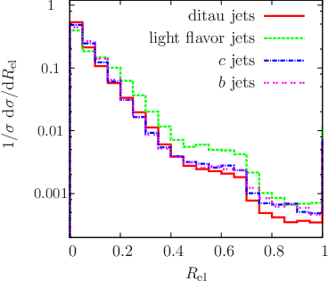
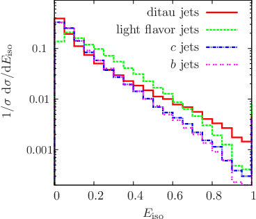
associated with a jet . Here the index runs over only the ecal cells of the jet, and is the angular distance of the th ecal cell from the jet. Note that both these quantities enter the tau-jet discriminating likelihood of Ref. [8] and play crucial roles in tagging a tau jet. As shown in Figure 2, ditau jets do not show sufficiently different profiles from ordinary QCD jets in either of these distributions. Consequently, it is evident that a naive application of single tau strategies to ditau jets results in a bad tagging performance.
Both and are designed to find a clean jet, i.e. a jet where most of the energy is deposited in only a few calorimeter cells that are also in close proximity to each other. A tau jet is such a jet since the hadronic decay products of the tau arise from a color-singlet state and the decay itself is an electroweak process. Although, we expect less radiation in a ditau jet compared to QCD [28], it is still not a clean jet. Unlike QCD jets, a ditau jet deposits energy in the calorimeter in a prong-like fashion – a feature which we exploit in our analysis. More specifically, we consider -subjettiness [29, 30], a derivative of the recently proposed observable -jettiness [31]. We use the definition of [30]
| (8) |
where the indices runs over the fat jet-constituents and the index denotes the number of required subjets. Note that in this definition, denotes the distance from the jet constituent to the subjet . -subjettiness†† † We do not perform a minimization procedure to retrieve a global event shape observable, but instead use the exclusive algorithm as implemented in FastJet on the jet’s constituents to cluster exactly subjets. is particularly successful in discriminating those jets that have a substructure of isolated collimated energy deposits from jets that have a more fanned out substructure. Actually, the ratios between different are found to be superior to plain distributions in discriminating jets with multiprong structures [30]. In the case of ditau jets, we find that , whether of the full calorimeter tower or of the ecal entries, works best (see Figure 3). It must be emphasized that in order to get small values of , does not need to match the number of charged decay products of the taus; rather it must match those of the pronounced energy deposits in the jet.
We find the ratio between a jet’s transverse momentum and mass, , to be another powerful discriminator between a ditau jet and an ordinary QCD jet. This quantity is sensitive to the size of the ”active area” of the jet (the area where radiation is measured), and to the alignment between hard radiation and jet axis. For the pencil-like structure of the ditau jets we expect larger values of than for QCD jets, which we confirm in Figure 5.
More interestingly, a distinct pattern of correlation is observed in the -subjettiness vs. plane for the ditau jets. For the QCD jets, as shown in Figure 4, increasing values of are correlated with increasing , whereas for ditau jets these are anti-correlated.
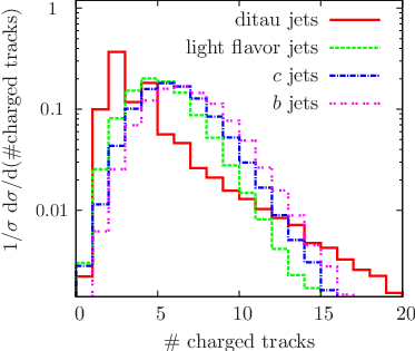
Before concluding this section let us also briefly mention that the number of charged tracks associated with a jet can play a crucial role in tagging ditau jets. In Figure 6 we have plotted the distribution of the number of charged tracks with . As expected, a much larger fraction of ditau jets contain or fewer tracks in them.

III Ditau jets at work: a case study
As a concrete phenomenological example, we apply the ditau sensitive observables from Sec. II to extract Higgses out of events via identifying ditau jets (candidates for particles). For a realistic discovery potential, however, we also need to be concerned about the rates. Consequently, we employ the discriminating powers of only and to isolate ditau jets after imposing realistic pre-selection requirements.
We again use the mass parameters quoted in Eq. (2) and assume . The signal events are characterized by two isolated hard leptons of identical flavor that reconstruct a boson, a couple of ditau jets, and a sizable amount of missing energy. Therefore, the biggest backgrounds to the signal events are due to , , and events. Note that +jets can also be an important background, since jet mismeasurement can give rise to a finite . On the other hand, +jets actually are SM-candle processes for getting a handle on these detector and jet energy-scale induced effects in a data-driven approach (see, e.g., Ref. [32]). It is impossible to realistically asses these systematic effects without carrying out the full detector simulation, especially because we are explicitly looking into the phase space region where the missing energy tends to be aligned with the leading jet (see below). Therefore, we have to rely on the experiments to estimate this contribution to the background. Given that the jet energy scale can be determined at the level of a few percent [33], we believe that this background can be reliably reduced and we do not include these events in our background analysis.
We produce the matched diboson+jet samples with Sherpa [34]. The QCD corrections to these processes have been provided recently in Ref. [35] (see also Ref. [36] for further details on precision diboson+jet phenomenology). We find the factors associated with () production to be using Vbfnlo [37], i.e. the QCD corrections reduce the leading order results in the considered phase space before subjets cuts are imposed. For the and production, there are currently no publicly available codes. However, it is known that the QCD corrections are qualitatively and qualitatively similar [35, 36], and we adopt the factor for events for the remaining backgrounds.
The sample is produced using Herwig++ [38]; we normalize to the NLO QCD cross section of pb [39]. The ditau signal events are generated using Pythia.
Even a very large ditau-jet tagging efficiency is still too low to compete with the large and backgrounds on an inclusive level if we also take into account a small mistagging probability. We, therefore, apply a number of -improving pre-selection criteria before we can use the ditau sensitive observables of the previous section. A similar strategy to reduce the backgrounds has been used in [40]. The cuts are summarized in Table 1 and we describe them in detail as follows:
| ditaus | |||||
| 1.00 | 1.00 | 1.00 | 1.00 | 1.00 | |
| 0.416 | 0.217 | 0.130 | 0.011 | 0.026 | |
| mass reconstruction with or | |||||
| 0.216 | 0.048 | 0.035 | 0.00019 | ||
| 0.199 | 0.0402 | 0.029 | 0.00019 | ||
| 0.172 | 0.033 | 0.021 | 0.00015 | ||
| (leading jet) | 0.125 | 0.011 | 0.0084 | ||
| (leading jet) | 0.083 | 0.0018 | 0.0020 | ||
| cross section [fb] | 1.32 | 0.45 | 1.83 | 0.18 | 0.29 |
- 1.
First, we require exactly two isolated leptons (cf. Sec. II) of identical flavor, each with . The leptons should reconstruct the mass within . This ensures that the event is triggerable and reduces the large and backgrounds.
- 2.
We impose staggered criteria on the two leptons and focus on the boosted kinematics with the Higgs recoiling against the in the signal sample, requiring .
- 3.
We require at least one anti- jet with a transverse momentum . We veto events that contain hard jets () close to the reconstructed (). We apply this cut to reduce the large background. In , to fake the boosted boson and pass the staggered cuts, one of the tops need to be boosted and its decay products need to be collimated. The veto removes events where the quark is close to the hard lepton.
- 4.
We require . The reconstructed missing transverse momentum vector additionally needs to be separated from the reconstructed by . The decays always produce neutrinos which result in a sizable amount of missing transverse energy. Together with the cuts on the lepton system, provides a good handle against the large background.
In the two final steps of the analysis we apply the results from Sec. II in a rectangular fashion:

- 5.
We require on the ecal level, and
- 6.
the leading jet is characterized by .
The two final steps are crucial in increasing the ditau signal over the contributing backgrounds. In total this leaves us with
| (9) |
and a signal cross section after cuts of
| (10) |
This means that we can achieve for . There is obviously a lot of parameter space left to relax our assumptions‡‡ ‡ For completeness, we note that there are certain parameter regions where the Higgs does have a sizable branching ratio to four taus [42]. . While this result is already good enough to constrain this specific model class, reconstructing the Higgs mass is more challenging. This is not a straightforward task since, due to the multiple tau decays, the missing transverse momentum’s direction is largely unconstrained. We impose an additional requirement of having at least two jets with () and calculate the so-called transverse cluster mass [41]
| (11) |
We, hereby, do not impose the two final selection criteria of Table 1 on the next-to-leading jet since we find that the next-to-leading jet may also be a single-tau jet or can be due to initial state radiation. Applying the ditau criteria reduces the signal cross section, but, in principle improves the mass resolution. We stress that the signal and the background have completely different shapes and that the bulk of the signal cross section clusters around the Higgs mass of . While the distributions are likely to be altered by detector effects, one can clearly use the low region to constrain or even measure a possible low- excess if the model is realized.
Note, reconstructing the mass of the Higgs is generically troublesome if the Higgs particle decays to partly invisible final states. In addition to that, hadronic observables which in principle allow to reconstruct the Higgs excess are heavily affected by initial state radiation and underlying event. The later also affects the definition of the transverse cluster mass since it explicitly depends on the jet mass. Further, initial state radiation can produce one of the two hardest jets in the event. As a result, the jacobian peak gets washed out significantly as shown in Figure 7 (compared to the good resolution in purely leptonic final states as considered in Ref. [41]). Nonetheless, side-band analyses seem very promising. When restricting we find and , which yields for .
IV Toward low ditau tagging
In this section we combine the (sub)jet observables of Sec. II.2 to a likelihood,
| (12) |
where the is the probability distribution of the respective observable in Figures 3 and 5. In Eq. (12) we have also included the number of charged tracks distribution, which adds additional discriminative power on top of and according to Figure 6.
From this likelihood we can construct a single quantity by a standard procedure (an exercise similar to that is done for -tagging [43]), which discriminates ditau jets from light flavor, and jets,
| (13) |
The function denotes the a priori probability of having a light flavor jet, a jet, or a jet. Therefore, . We choose these probabilities by counting the color and flavor degrees and completely disregard the parton distributions in the initial states:
| (14) |
Since the distributions of the QCD jets are less sensitive to the flavor content of the jets, this choice has only a small impact on the actual distribution of . The result of the choice in Eq. (14) is shown in Fig. 8. Considering jets with with gives a ditau-tagging efficiency of () and with an average mistagging probability of ( ) if charged tracks are included (not included).


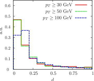
The tagging efficiency is, of course, a function of the considered jet’s transverse momentum as shown in Figure 9. For larger transverse momenta, looses its discriminative power, while the discriminative features of the observable remain intact.
V Summary and Conclusions
Non-standard Higgs sectors with non-standard Higgs decays require dedicated analysis strategies in order not to miss evidence of new physics when analyzing early LHC data. In this letter we have argued, that straightforwardly applying tau recognition algorithms to jets which actually consist of a boosted tau pair does not lead to a satisfactory signal-over-background discrimination. Consequently, current analysis strategies are not suitable to cope with these signatures which might well arise in scenarios of strong interactions, the NMSSM or in hidden-valley-type models.
We have shown that the combination of only two observable, -subjettiness (in particular ) and does serve to highly lift the degeneracy of ditau jets and QCD jets of all kind. The combination of both observables encodes orthogonal information on the ditaus’ distinct radiation and decay pattern.
We have applied these results in a phenomenological analysis of for boosted kinematics and have shown that constraints can be formulated for small integrated luminosities and that the Higgs mass for the chosen parameters can, in principle, be reconstructed. More specifically, we find that the Higgs signal becomes statistically significant for luminosities leaving enough space to compensate smaller branching ratios in more realistic scenarios.
Constructing a toy ditau tagger based on the two observables, augmented by the number of charged tracks distribution in a likelihood approach, we find a high tagging efficiency with an acceptably small mistagging probability, not too sensitive on the considered jet’s .
Of course, our results are subject to modifications when confronted with all contributing experimental uncertainties and mass setups different from Eq. (2). However, our findings strongly motivate a more detailed investigation within a full detector simulation framework.
Acknowledgments — CE thanks Bob McElrath and Tilman Plehn for discussions and Jeannette Bloch-Ditzinger for all the enjoyable coffee breaks. TSR thanks Anna Goussiou for conversations. CE and MS thank the Fermilab Theoretical Physics Department for hospitality during the time when parts of this work were completed.
The simulations underlying this study have been performed in parts on bwGRiD (http://www.bw-grid.de), member of the German D-Grid initiative, funded by the Ministry for Education and Research (Bundesministerium für Bildung und Forschung) and the Ministry for Science, Research and Arts Baden-Württemberg (Ministerium für Wissenschaft, Forschung und Kunst Baden-Württemberg). We thank Daniel Steck and Jeremy Thorn for the use of the Quantum Control computer cluster at the University of Oregon. MS was supported by the US Department of Energy under contract number DE-FG02-96ER40969. TSR was supported in part by the US Department of Energy under contract number DE-FGO2-96ER40956.
References
- [1] G. Aad et al. [ATLAS Collaboration], JINST 3 (2008) S08003.
- [2] G. L. Bayatian et al. [CMS Collaboration], J. Phys. G 34 (2007) 995.
- [3] C. P. Buszello, I. Fleck, P. Marquard and J. J. van der Bij, Eur. Phys. J. C 32 (2004) 209; Y. Gao, A. V. Gritsan, Z. Guo, K. Melnikov, M. Schulze and N. V. Tran, Phys. Rev. D 81, 075022 (2010); A. De Rujula, J. Lykken, M. Pierini, C. Rogan and M. Spiropulu, Phys. Rev. D 82 (2010) 013003; C. Englert, C. Hackstein and M. Spannowsky, Phys. Rev. D 82 (2010) 114024.
- [4] J. M. Butterworth, A. R. Davison, M. Rubin and G. P. Salam, Phys. Rev. Lett. 100 (2008) 242001.
- [5] D. E. Soper, M. Spannowsky, JHEP 1008, 029 (2010).
- [6] G. D. Kribs, A. Martin, T. S. Roy and M. Spannowsky, Phys. Rev. D 81 (2010) 111501; G. D. Kribs, A. Martin, T. S. Roy and M. Spannowsky, Phys. Rev. D 82 (2010) 095012
- [7] G. D. Kribs, A. Martin and T. S. Roy, arXiv:1012.2866 [hep-ph].
- [8] M. Heldmann, D. Cavalli, ATL-PHYS-PUB-2006-008, ATL-COM-PHYS-2006-010.
- [9] D. L. Rainwater, D. Zeppenfeld and K. Hagiwara, Phys. Rev. D 59 (1998) 014037; T. Plehn, D. L. Rainwater and D. Zeppenfeld, B. Mellado, W. Quayle and S. L. Wu, Phys. Lett. B 611 (2005) 60.
- [10] A. Martin and T. S. Roy, arXiv:1103.3504 [hep-ph].
- [11] R. Dermisek and J. F. Gunion, Phys. Rev. Lett. 95 (2005) 041801; R. Dermisek, J. F. Gunion and B. McElrath, Phys. Rev. D 76 (2007) 051105; R. Dermisek and J. F. Gunion, Phys. Rev. D 81 (2010) 075003.
- [12] M. Maniatis, Int. J. Mod. Phys. A 25 (2010) 3505; U. Ellwanger, C. Hugonie and A. M. Teixeira, Phys. Rept. 496 (2010) 1; S. Chang, P. J. Fox, N. Weiner, JHEP 0608, 068 (2006).
- [13] G. F. Giudice, C. Grojean, A. Pomarol and R. Rattazzi, JHEP 0706 (2007) 045; B. Bellazzini, C. Csaki, A. Falkowski and A. Weiler, Phys. Rev. D 80 (2009) 075008.
- [14] R. Contino, C. Grojean, M. Moretti, F. Piccinini and R. Rattazzi, JHEP 1005 (2010) 089; J. R. Espinosa, C. Grojean and M. Muhlleitner, JHEP 1005 (2010) 065; A. Falkowski, D. Krohn, L. T. Wang, J. Shelton and A. Thalapillil, arXiv:1006.1650 [hep-ph]; R. Grober and M. Muhlleitner, arXiv:1012.1562 [hep-ph].
- [15] R. Schabinger and J. D. Wells, Phys. Rev. D 72 (2005) 093007; B. Patt and F. Wilczek, arXiv:hep-ph/0605188; M. J. Strassler and K. M. Zurek, Phys. Lett. B 651, 374 (2007).
- [16] S. Bock, R. Lafaye, T. Plehn, M. Rauch, D. Zerwas and P. M. Zerwas, Phys. Lett. B 694, 44 (2010); C. Englert, T. Plehn, D. Zerwas and P. M. Zerwas, arXiv:1106.3097 [hep-ph].
- [17] T. Aaltonen et al. [CDF Collaboration], Phys. Rev. Lett. 100 (2008) 161802; V. M. Abazov et al. [D0 Collaboration], Phys. Rev. Lett. 101 (2008) 241801; A. Lenz et al., Phys. Rev. D 83 (2011) 036004.
- [18] V. M. Abazov et al. [D0 Collaboration], Phys. Rev. D 82 (2010) 032001.
- [19] A. Dighe, A. Kundu and S. Nandi, Phys. Rev. D 82 (2010) 031502.
- [20] Y. Bai and A. E. Nelson, Phys. Rev. D 82 (2010) 114027.
- [21] A. Katz, M. Son and B. Tweedie, arXiv:1011.4523 [hep-ph].
- [22] M. Carena, T. Han, G. Y. Huang and C. E. M. Wagner, JHEP 0804, 092 (2008).
- [23] T. Sjostrand, S. Mrenna and P. Z. Skands, JHEP 0605, 026 (2006); http://home.thep.lu.se/~torbjorn/Pythia.html.
- [24] J. Conway et al., http://www.physics.ucdavis.edu/~conway/research/software/pgs/pgs.html.
- [25] C. R. Chen, M. M. Nojiri and W. Sreethawong, JHEP 1011 (2010) 012.
- [26] M. Cacciari and G. P. Salam, Phys. Lett. B 641, 57 (2006); M. Cacciari, G. P. Salam and G. Soyez, http://fastjet.fr.
- [27] K. Nakamura et al. [Particle Data Group], J. Phys. G 37 (2010) 075021.
- [28] G. Marchesini, B. R. Webber, Nucl. Phys. B238, 1 (1984); J. Gallicchio and M. D. Schwartz, Phys. Rev. Lett. 105 (2010) 022001; A. Hook, M. Jankowiak and J. G. Wacker, arXiv:1102.1012 [hep-ph]; D. E. Soper, M. Spannowsky, arXiv:1102.3480 [hep-ph].
- [29] J. H. Kim, Phys. Rev. D 83 (2011) 011502.
- [30] J. Thaler and K. Van Tilburg, JHEP 1103 (2011) 015.
- [31] I. W. Stewart, F. J. Tackmann, W. J. Waalewijn, Phys. Rev. Lett. 105, 092002 (2010).
- [32] The CMS Collaboration, CMS PAS SUS-10-001; The CMS collaboration, CMS-PAS-JME-09-005; The Atlas collaboration, ATL-PHYS-PUB-2009-015.
- [33] see, e.g., The Atlas collaboration, ATLAS-CONF-2010-056.
- [34] T. Gleisberg, S. Hoeche, F. Krauss, M. Schonherr, S. Schumann, F. Siegert and J. Winter, JHEP 0902, 007 (2009); S. Schumann and F. Krauss, JHEP 0803 (2008) 038; T. Gleisberg and S. Hoeche, JHEP 0812 (2008) 039; M. Schonherr and F. Krauss, JHEP 0812, 018 (2008), http://www.sherpa-mc.de/.
- [35] S. Dittmaier, S. Kallweit and P. Uwer, Phys. Rev. Lett. 100, 062003 (2008); J. M. Campbell, R. Keith Ellis and G. Zanderighi, JHEP 0712 (2007) 056; T. Binoth, T. Gleisberg, S. Karg, N. Kauer and G. Sanguinetti, Phys. Lett. B 683 (2010) 154; F. Campanario, C. Englert, S. Kallweit, M. Spannowsky and D. Zeppenfeld, JHEP 1007 (2010) 076.
- [36] F. Campanario, C. Englert, M. Spannowsky and D. Zeppenfeld, Europhys. Lett. 88 (2009) 11001; F. Campanario, C. Englert and M. Spannowsky, Phys. Rev. D 82 (2010) 054015; F. Campanario, C. Englert and M. Spannowsky, Phys. Rev. D 83 (2011) 074009.
- [37] K. Arnold et al., Comput. Phys. Commun. 180 (2009) 1661, http://www-itp.particle.uni-karlsruhe.de/~vbfnloweb.
- [38] M. Bahr et al., Eur. Phys. J. C 58 (2008) 639; http://projects.hepforge.org/herwig/.
- [39] M. Cacciari, S. Frixione, M. L. Mangano, P. Nason and G. Ridolfi, JHEP 0809, 127 (2008).
- [40] B. Batell, J. Pradler and M. Spannowsky, arXiv:1105.1781 [hep-ph].
- [41] V. D. Barger, T. Han and J. Ohnemus, Phys. Rev. D 37 (1988) 1174.
- [42] R. Dermisek, J. F. Gunion, Phys. Rev. D81 (2010) 075003; F. Domingo, U. Ellwanger, JHEP 1106 (2011) 067.
- [43] C. Weiser, CMS NOTE 2006/014.