跳到论文正文
W Papers独立论文阅读器 arXiv:1106.4539 论文正文 计算阅读时间 · 0%
引用这篇论文根据当前论文元数据生成,正式投稿前建议核对。


License: arXiv.org perpetual non-exclusive license
arXiv:1106.4539v1 [nucl-th] 22 Jun 2011

The two-nucleon electromagnetic charge operator in chiral effective field theory (χ\chiEFT) up to one loop

S. Pastorea{}^{\,{\rm a}}, L. Girlandab,c{}^{\,{\rm b,c}}, R. Schiavillad,e{}^{\,{\rm d,e}}, and M. Vivianif{}^{\,{\rm f}} Affiliation: aPhysics Division, Argonne National Laboratory, IL 60439, USA
b{}^{\,{\rm b}}Department of Physics, Università del Salento, I-73100 Lecce, Italy
c{}^{\,{\rm c}}INFN Sezione di Lecce, I-73100 Lecce, Italy
dDepartment of Physics, Old Dominion University, Norfolk, VA 23529, USA
eJefferson Lab, Newport News, VA 23606, USA
f{}^{\,{\rm f}}INFN Sezione di Pisa, I-56127 Pisa, Italy
August 24, 2026
Abstract

The electromagnetic charge operator in a two-nucleon system is derived in chiral effective field theory (χ\chiEFT) up to order e​Qe\,Q (or N4LO), where QQ denotes the low-momentum scale and ee is the electric charge. The specific form of the N3LO and N4LO corrections from, respectively, one-pion-exchange and two-pion-exchange depends on the off-the-energy-shell prescriptions adopted for the non-static terms in the corresponding potentials. We show that different prescriptions lead to unitarily equivalent potentials and accompanying charge operators. Thus, provided a consistent set is adopted, predictions for physical observables will remain unaffected by the non-uniqueness associated with these off-the-energy-shell effects.

pacs
12.39.Fe, 13.40.-f

I Introduction

The chiral symmetry exhibited by quantum chromodynamics (QCD) dictates that the pion couples to baryons, such as nucleons and Δ\Delta-isobars, by powers of its momentum QQ. As a consequence, the Lagrangian describing these interactions can be expanded in powers of Q/ΛχQ/\Lambda_{\chi}, where Λχ∼1\Lambda_{\chi}\sim 1 GeV specifies the chiral-symmetry breaking scale. Thus, classes of Lagrangians emerge, each characterized by a given power of Q/ΛχQ/\Lambda_{\chi} and each involving a certain number of unknown coefficients, so called low-energy constants, which are then determined by fits to experimental data (see, for example, the review papers [1] and [2], and references therein). This approach, known as chiral effective field theory (χ\chiEFT), can be justifiably argued to have put low-energy nuclear physics on a more fundamental basis by providing, on the one hand, a direct connection between the symmetries of QCD—in particular, chiral symmetry—and the strong and electroweak interactions in nuclei, and, on the other hand, a practical calculational scheme susceptible, in principle, of systematic improvement.

The model for the nuclear electromagnetic current—the space-like part of the four current—in χ\chiEFT up to one loop was derived originally by Park et al. [3], using covariant perturbation theory. In the last couple of years, two independent derivations, based on time-ordered perturbation theory (TOPT), have appeared in the literature, one by the present authors [4] and the other by Kölling et al. [5]. There are technical differences in the implementation of TOPT, which relate to the treatment of reducible diagrams and are documented in considerable detail in the above papers. However, the resulting expressions in Refs. [4] and [5] for the two-pion-exchange currents (the only ones considered by the authors of Ref. [5]) are in agreement with each other, but differ from those of Ref. [3], in particular in the isospin structure of the M​1M1 operator associated with the one-loop corrections—see Pastore et al. (2009) [4] for a comparison and analysis of these differences.

Kölling et al. also provided the first treatment of loop corrections to the nuclear charge operator—the time-like part of the four current—associated with two-pion exchange mechanisms. Of course, there had been earlier studies of the two-nucleon charge operator, notably those of Refs. [6, 7, 8], but they had been limited to its isoscalar component, and therefore had only retained tree-level corrections (the two-pion-exchange loop contributions are isovector). These earlier studies also included predictions for the charge and quadrupole form factors of the deuteron, which were in reasonable agreement with data obtained from measurements of elastic electron-deuteron scattering cross sections at low-momentum transfer.

The primary objective of the present work is to extend the formalism developed in Refs. [4, 9] to derive systematically the two-nucleon electromagnetic charge operator in χ\chiEFT, including up to one loop corrections. As we shall see below, this is not a straight-forward task, since the derivation of such an operator necessarily entails the study of non-static contributions to the one-pion-exchange (OPE) and two-pion-exchange (TPE) potentials. In the OPE sector, this inter-connection between non-static contributions and the charge operator was investigated long ago by Friar [10] in the context of a Foldy-Wouthuysen reduction procedure and a time-dependent perturbation theory, which consistently retained corrections up to order (v/c)2(v/c)^{2}. In particular, Friar showed that i) the charge operators so derived depend on the specific, but arbitrary, off-the-energy extension—i.e., on the corrections beyond the static limit, such as those induced by retardation effects—adopted for the OPE potential, and that ii) these different operators (and corresponding OPE potentials) are related to each other by a unitary transformation and, therefore, their intrinsic lack of uniqueness has no consequence on the predictions for physical observables.

In this paper, we examine these issues from a χ\chiEFT perspective. We are interested in constructing the charge operators up to one loop and, hence, need to include non-static corrections not only in the OPE, but also in the TPE potential. We show that the resulting operators, while not unique because of the off-the-energy-shell ambiguity referred to above, are nevertheless related to each other by a unitary transformation. Thus the present study puts Friar’s original considerations in the modern framework of χ\chiEFT and extends them to the TPE sector. In Sec. II and App. A we list those terms in the chiral Lagrangians (and corresponding interaction Hamiltonians) that are relevant to our purpose here. In Sec. III we provide an overview of the derivation of the OPE and TPE potentials and charge operators. Specifically, we explore the connection between the amplitude calculated in χ\chiEFT and the strong and electromagnetic potentials, which are derived from it and are used in quantum-mechanical formulations, based on the Lippmann-Schwinger or Schrödinger equations. Power counting allows us to establish a criterion to make this connection precise. Elsewhere [9, 4], we have referred to the latter as “accounting for recoil-corrected reducible contributions.” The present formulation is especially apt to shed light on the inter-dependence between charge operators and potentials (at the OPE and TPE level), and the associated ambiguity arising from off-the-energy-shell extrapolations prescribed for the latter.

In Sec. III we also provide an explicit expression for the unitary transformation, and show, in particular, that different (non-static) versions of the TPE potential are unitarily equivalent. As mentioned above, in the OPE sector this result has been known for a while [10, 11].

Section IV contains a summary of the derivation of the two-nucleon charge operators up to order e​Q 0e\,Q^{\,0} included, or next-to-next-to-next-to-leading order (N3LO in short), where ee is the proton electric charge and QQ denotes generically the low-momentum scale. No loops enter at this order. The different forms of the OPE charge operator at N3LO exhibit the same unitary equivalence as the non-static corrections to the OPE potential at order Q2Q^{2} (N2LO)—this too is well known [10, 11], albeit in a different context.

In Sec. V we discuss the static one-loop corrections to the charge operator at N4LO (e​Qe\,Q). In particular, we list those corresponding to two different off-the-energy-shell prescriptions for the OPE and TPE potentials, and show that they are unitarily equivalent. A fairly detailed account of their derivation is provided in App. B. The loop integrals entering the individual terms at N4LO are ultraviolet divergent; however, their sum is finite, in particular it vanishes in the limit in which the momentum 𝐪{\bf q} carried by the electromagnetic field is zero. This was to be expected, since i) symmetry arguments prevent the presence of counterterms at this order (and therefore the possibility of re-absorbing ensuing divergencies into them), and ii) charge conservation demands that at 𝐪=0{\bf q}=0 the charge operator merely counts the number of charged particles (i.e., protons) in the system—a requirement already fulfilled at LO. Summary and conclusions are presented in Sec. VI, while, for future convenience, we give the configuration space representation of the N4LO charge operators in App. C.

II Relevant interaction Hamiltonians

Here we only list the interaction Hamiltonians relevant for the derivation of the nuclear electromagnetic charge operator up to order e​Qe\,Q (N4LO), see App. A for notation and a summary of the corresponding Lagrangians [12, 13]:

Hπ​N\displaystyle\!H_{\pi N}\!\! =\displaystyle= ∫d​𝐱​N†​[gA​τaFπ​𝝈⋅∇πa+𝝉Fπ2⋅(𝝅×∂ 0𝝅)]​N,\displaystyle\!\!\!\int\!\!\!{\rm d}{\bf x}N^{\dagger}\Big[\frac{g_{A}\,\tau_{a}}{F_{\pi}}{\bm{\sigma}}\cdot{\bm{\nabla}}\pi_{a}\!+\!\frac{{\bm{\tau}}}{F_{\pi}^{2}}\cdot({\bm{\pi}}\times\partial^{\,0}{\bm{\pi}})\Big]\!N, (1)
Hγ​N\displaystyle H_{\gamma N}\!\! =\displaystyle= e∫d𝐱N†[eNA0−2​μN−eN8​mN2[(∇2A0)\displaystyle\!\!e\int\!\!{\rm d}{\bf x}\,N^{\dagger}\Big[e_{N}\,A^{0}-\frac{2\,\mu_{N}-e_{N}}{8\,m_{N}^{2}}\big[({\bm{\nabla}}^{2}A^{0}) (2)
+\displaystyle+ 𝝈×(∇A0)⋅∇→−∇←⋅𝝈×(∇A0)]]N,\displaystyle{\bm{\sigma}}\times({\bm{\nabla}}A^{0})\cdot\overrightarrow{\bm{\nabla}}-\overleftarrow{\bm{\nabla}}\cdot{\bm{\sigma}}\times({\bm{\nabla}}A^{0})\big]\Big]N\ ,
Hγ​π\displaystyle H_{\gamma\pi}\!\! =\displaystyle= e​∫d​𝐱​A0​(𝝅×∂0𝝅)z,\displaystyle\!\!e\int\!\!{\rm d}{\bf x}\,A^{0}\,\left({\bm{\pi}}\times\partial_{0}{\bm{\pi}}\right)_{z}\ , (3)
Hγ​π​N\displaystyle H_{\gamma\pi N}\!\! =\displaystyle= e∫d𝐱N†𝝈⋅(∇A0)[gA2​mN​Fπ(𝝉⋅𝝅+πz)\displaystyle\!\!e\int\!\!{\rm d}{\bf x}\,N^{\dagger}\,{\bm{\sigma}}\cdot\left({\bm{\nabla}}A^{0}\right)\,\Big[\frac{g_{A}}{2\,m_{N}F_{\pi}}\left({\bm{\tau}}\cdot{\bm{\pi}}+\pi_{z}\right) (4)
+\displaystyle+ 1Fπ(2d20+2d21−d22)(𝝉×∂ 0𝝅)z]N.\displaystyle\frac{1}{F_{\pi}}\,(2\,d_{20}+2\,d_{21}-d_{22})\,({\bm{\tau}}\times\partial^{\,0}{\bm{\pi}})_{z}\,\Big]\,N\ .

The resulting vertices behave, relative to the low-momentum scale QQ, in the following way: Hπ​N∼QH_{\pi N}\sim Q; first term in Hγ​N∼e​Q 0H_{\gamma N}\sim e\,Q^{\,0}, remaining ones ∼e​Q2\sim e\,Q^{2}; Hγ​π∼e​QH_{\gamma\pi}\sim e\,Q; first term in Hγ​π​N∼e​QH_{\gamma\pi N}\sim e\,Q, second one ∼e​Q2\sim e\,Q^{2}. There is also a contact interaction,

HCT\displaystyle H_{\rm CT} =\displaystyle= 12∫d𝐱[CS(N†N)(N†N)\displaystyle\frac{1}{2}\int{\rm d}{\bf x}\,\Big[C_{S}\left(N^{\dagger}N\right)\left(N^{\dagger}N\right) (5)
+\displaystyle+ CT(N†𝝈N)⋅(N†𝝈N)],\displaystyle C_{T}\left(N^{\dagger}{\bm{\sigma}}N\right)\cdot\left(N^{\dagger}{\bm{\sigma}}N\right)\Big]\ ,

which enters the derivation of the N4LO charge operator. The accompanying vertex scales as Q 0Q^{\,0}.

III From amplitudes to potentials

We begin by considering the conventional perturbative expansion for the two-nucleon (N​NNN) scattering amplitude

⟨f∣T∣i⟩=⟨f∣H1​∑n=1∞(1Ei−H0+i​η​H1)n−1∣i⟩,\langle f\mid T\mid i\rangle=\langle f\mid H_{1}\sum_{n=1}^{\infty}\left(\frac{1}{E_{i}-H_{0}+i\,\eta}H_{1}\right)^{n-1}\mid i\rangle\ , (6)

where ∣i⟩\mid i\rangle and ∣f⟩\mid f\rangle represent the initial and final two-nucleon states of energy Ei=EfE_{i}=E_{f}, H0H_{0} is the Hamiltonian describing free pions and nucleons, and H1H_{1} is the Hamiltonian describing interactions among these particles (Sec. II). The evaluation of this amplitude is carried out in practice by inserting complete sets of H0H_{0} eigenstates between successive terms of H1H_{1}. Power counting is then used to organize the expansion in powers of Q/Λχ≪1Q/\Lambda_{\chi}\ll 1, where Λχ≃1\Lambda_{\chi}\simeq 1 GeV is the typical hadronic mass scale.

In the perturbative series, Eq. (6), a generic (reducible or irreducible) contribution is characterized by a certain number, say NN, of vertices, each scaling as Qαi×Q−βi/2Q^{\alpha_{i}}\times Q^{-\beta_{i}/2} (ii=1,…,N1,\dots,N), where αi\alpha_{i} is the power counting implied by the relevant interaction Hamiltonian and βi\beta_{i} is the number of pions in and/or out of the vertex, a corresponding NN–1 number of energy denominators, and possibly LL loops [9]. Out of these NN–1 energy denominators, NKN_{K} of them will involve only nucleon kinetic energies, which scale as Q2Q^{2}, and the remaining N−NK−1N-N_{K}-1 will involve, in addition, pion energies, which are of order QQ. Loops, on the other hand, contribute a factor Q3Q^{3} each, since they imply integrations over intermediate three momenta. Hence the power counting associated with such a contribution is

(∏i=1NQαi−βi/2)×[Q−(N−NK−1)​Q−2​NK]×Q3​L.\left(\prod_{i=1}^{N}Q^{\alpha_{i}-\beta_{i}/2}\right)\times\left[Q^{-(N-N_{K}-1)}\,Q^{-2N_{K}}\right]\times Q^{3L}\ . (7)

Clearly, each of the N−NK−1N-N_{K}-1 energy denominators can be further expanded as

1Ei−EI−ωπ=−1ωπ[1\displaystyle\frac{1}{E_{i}-E_{I}-\omega_{\pi}}=-\frac{1}{\omega_{\pi}}\bigg[1 +\displaystyle+ Ei−EIωπ\displaystyle\frac{E_{i}-E_{I}}{\omega_{\pi}} (8)
+\displaystyle+ (Ei−EI)2ωπ2+…],\displaystyle\frac{(E_{i}-E_{I})^{2}}{\omega^{2}_{\pi}}+\dots\bigg]\ ,

where EIE_{I} denotes the kinetic energy of the intermediate two-nucleon state, and ωπ\omega_{\pi} the pion energy (or energies, as the case may be)—the ratio (Ei−EI)/ωπ(E_{i}-E_{I})/\omega_{\pi} is of order QQ.

The QQ-scaling of the interaction vertices and the considerations above show that TT admits the following expansion:

T=T(0)+T(1)+T(2)+…,T=T^{(0)}+T^{(1)}+T^{(2)}+\dots\ , (9)

where T(n)∼QnT^{(n)}\sim Q^{n}. For example, the time-ordered diagrams contributing to T(0)T^{(0)} and T(1)T^{(1)} are illustrated in Fig. 1, where the pion line (pion line with a crossed circle) indicates that only the leading −1/ωπ-1/\omega_{\pi} (next-to-leading −(Ei−EI)/ωπ2-(E_{i}-E_{I})/\omega^{2}_{\pi}) term is retained in the expansion of the associated energy denominator, Eq. (8). Except for App. B, this notation will not be used any further below, but it is understood that energy denominators involving pions are expanded as in Eq. (8).

Our objective is to derive a two-nucleon potential vv which, when iterated in the Lippmann-Schwinger (LS) equation,

v+v​G0​v+v​G0​v​G0​v+…,v+v\,G_{0}\,v+v\,G_{0}\,v\,G_{0}\,v+\dots\ , (10)

leads to the TT-matrix in Eq. (9), order by order in the power counting. In practice, this requirement can only be satisfied up to a given order n∗n^{*}, and the resulting potential, when inserted into the LS (or Schrödinger) equation, will generate contributions of order n>n∗n>n^{*}, which do not match T(n)T^{(n)}. In Eq. (10), G0G_{0} denotes the free two-nucleon propagator, G0=1/(Ei−EI+i​η)G_{0}=1/(E_{i}-E_{I}+i\,\eta), and we assume that

v=v(0)+v(1)+v(2)+…,v=v^{(0)}+v^{(1)}+v^{(2)}+\dots\ , (11)

where the yet to be determined v(n)v^{(n)} is of order QnQ^{n}. We also note that, generally, a term like v(m)​G0​v(n)v^{(m)}\,G_{0}\,v^{(n)} is of order Qm+n+1Q^{m+n+1}, since G0G_{0} is of order Q−2Q^{-2} and the implicit loop integration brings in a factor Q3Q^{3}. Having established the above power counting, we obtain

v(0)\displaystyle v^{(0)} =\displaystyle= T(0),\displaystyle T^{(0)}\ , (12)
v(1)\displaystyle v^{(1)} =\displaystyle= T(1)−[v(0)​G0​v(0)],\displaystyle T^{(1)}-\left[v^{(0)}\,G_{0}\,v^{(0)}\right]\ , (13)
v(2)\displaystyle v^{(2)} =\displaystyle= T(2)−[v(0)​G0​v(0)​G0​v(0)]\displaystyle T^{(2)}-\left[v^{(0)}\,G_{0}\,v^{(0)}\,G_{0}\,v^{(0)}\right] (14)
−[v(1)​G0​v(0)+v(0)​G0​v(1)],\displaystyle\qquad-\left[v^{(1)}\,G_{0}\,v^{(0)}+v^{(0)}\,G_{0}\,v^{(1)}\right]\ ,
v(3)\displaystyle v^{(3)} =\displaystyle= T(3)−[v(0)​G0​v(0)​G0​v(0)​G0​v(0)]\displaystyle T^{(3)}-\left[v^{(0)}\,G_{0}\,v^{(0)}\,G_{0}\,v^{(0)}\,G_{0}\,v^{(0)}\right] (15)
−[v(1)​G0​v(0)​G0​v(0)+permutations]\displaystyle\qquad-\left[v^{(1)}\,G_{0}\,v^{(0)}\,G_{0}\,v^{(0)}+{\rm permutations}\right]
−[v(2)​G0​v(0)+v(0)​G0​v(2)]\displaystyle\qquad-\left[v^{(2)}\,G_{0}\,v^{(0)}+v^{(0)}\,G_{0}\,v^{(2)}\right]
−[v(1)​G0​v(1)],\displaystyle\qquad-\left[v^{(1)}\,G_{0}\,v^{(1)}\right]\ ,

where v(n)v^{(n)} is the “recoil-corrected” two-nucleon potential explicitly constructed in Refs. [9, 4] up to order n=2n=2, or N2LO. The LO term, v(0)v^{(0)}, consists of (static) one-pion-exchange (OPE) and contact interactions, while the NLO term, v(1)v^{(1)}, vanishes, since the contributions of diagrams (d) and (e) in T(1)T^{(1)}, illustrated in Fig. 1, add up to zero, while the remaining diagrams represent iterations of v(0)v^{(0)}, whose contributions are exactly canceled by [v(0)​G0​v(0)]\left[v^{(0)}\,G_{0}\,v^{(0)}\right]—complete or partial cancellations of this type persist at higher (n≥2n\geq 2) orders. The N2LO term, which follows from Eq. (14), contains two-pion-exchange (TPE) and contact (involving two gradients of the nucleon fields) interactions. It is derived in Ref. [4]. However, there is a recoil correction of order n=2n=2 to the OPE potential, which was ignored in that paper. In momentum space, it is given by

vπ(2)​(ν=0)=vπ(0)​(𝐤)​(E1′−E1)2+(E2′−E2)22​ωk2,v^{(2)}_{\pi}(\nu=0)=v^{(0)}_{\pi}({\bf k})\,\,\frac{(E_{1}^{\,\prime}-E_{1})^{2}+(E_{2}^{\,\prime}-E_{2})^{2}}{2\,\omega_{k}^{2}}\ , (16)

where vπ(0)v^{(0)}_{\pi} is the LO OPE potential,

vπ(0)(𝐤)=−gA2Fπ2𝝉1⋅𝝉2𝝈1⋅𝐤​𝝈2⋅𝐤ωk2,v^{(0)}_{\pi}({\bf k})=-\frac{g_{A}^{2}}{F_{\pi}^{2}}\,{\bm{\tau}}_{1}\cdot{\bm{\tau}}_{2}\,\frac{{\bm{\sigma}}_{1}\cdot{\bf k}\,\,{\bm{\sigma}}_{2}\cdot{\bf k}}{\omega_{k}^{2}}\ , (17)

𝐤=𝐩1−𝐩1′=𝐩2′−𝐩2{\bf k}={\bf p}_{1}-{\bf p}^{\prime}_{1}={\bf p}_{2}^{\prime}-{\bf p}_{2} is the momentum transfer, and 𝐩j{\bf p}_{j} and EjE_{j} (𝐩j′{\bf p}^{\prime}_{j} and Ej′E_{j}^{\,\prime}) are the initial (final) momentum and energy of nucleon jj. Obviously, on the energy shell Ei=EfE_{i}=E_{f} implicit in Eq. (14), the above expression is equivalent to one in which, for example,

vπ(2)​(ν=1)=−vπ(0)​(𝐤)​(E1′−E1)​(E2′−E2)ωk2.v^{(2)}_{\pi}(\nu=1)=-v^{(0)}_{\pi}({\bf k})\,\,\frac{(E_{1}^{\,\prime}-E_{1})\,(E_{2}^{\,\prime}-E_{2})}{\omega_{k}^{2}}\ . (18)

In fact, there is an infinite class of vπ(2)​(ν)v_{\pi}^{(2)}(\nu) corrections—labeled by the parameter ν\nu [10, 14, 11]—which, while equivalent on the energy-shell, are different off the energy-shell, and therefore lead to different potentials v(3)​(ν)v^{(3)}(\nu) in Eq. (15). Indeed, for the choices of vπ(2)​(ν)v_{\pi}^{(2)}(\nu) in Eqs. (16) and (18) the corresponding corrections to the TPE term (from direct and crossed box diagrams), v2​π(3)​(ν)v^{(3)}_{{2\pi}}(\nu), read

v2​π(3)​(ν=0)\displaystyle v_{{2\pi}}^{(3)}(\nu=0)\!\! =\displaystyle= −gA42​Fπ4(3+2𝝉1⋅𝝉2)∫𝐪1(𝝈1⋅𝐪2)(𝝈1⋅𝐪1)\displaystyle\!\!-\frac{g_{A}^{4}}{2\,F_{\pi}^{4}}(3+2\,{\bm{\tau}}_{1}\cdot{\bm{\tau}}_{2})\int_{{\bf q}_{1}}({\bm{\sigma}}_{1}\cdot{\bf q}_{2})({\bm{\sigma}}_{1}\cdot{\bf q}_{1}) (19)
×\displaystyle\times (𝝈2⋅𝐪1)​(𝝈2⋅𝐪2)​(E1−E~1+E2′−E~2′ω14​ω22CLOSE\displaystyle\!\!({\bm{\sigma}}_{2}\cdot{\bf q}_{1})({\bm{\sigma}}_{2}\cdot{\bf q}_{2})\bigg(\frac{E_{1}-\widetilde{E}_{1}+E_{2}^{\prime}-\widetilde{E}_{2}^{\prime}}{\omega_{1}^{4}\,\omega_{2}^{2}}
+\displaystyle+ OPENE1′−E~1+E2−E~2′ω12​ω24),\displaystyle\!\!\frac{E_{1}^{\prime}-\widetilde{E}_{1}+E_{2}-\widetilde{E}_{2}^{\prime}}{\omega_{1}^{2}\,\omega_{2}^{4}}\bigg)\ ,

and

v2​π(3)​(ν=1)\displaystyle\!\!\!v_{{2\pi}}^{(3)}(\nu=1)\!\! =\displaystyle= v2​π(3)​(ν=0)+12​∫𝐪1vπ(0)​(𝐪2)​vπ(0)​(𝐪1)\displaystyle\!\!v_{{2\pi}}^{(3)}(\nu=0)+\frac{1}{2}\int_{{\bf q}_{1}}v_{\pi}^{(0)}({\bf q}_{2})\,v_{\pi}^{(0)}({\bf q}_{1}) (20)
×\displaystyle\times (E1+E2−E~1−E~2)​(1ω12+1ω22),\displaystyle\!\!\!\left(E_{1}+E_{2}-\widetilde{E}_{1}-\widetilde{E}_{2}\right)\!\left(\frac{1}{\omega_{1}^{2}}+\frac{1}{\omega_{2}^{2}}\right),

where, as indicated in panel (a) of Fig. 4 (App. B), 𝐪1{\bf q}_{1} and 𝐪2{\bf q}_{2} (ω1\omega_{1} and ω2\omega_{2}) are the momenta (energies) of the two exchanged pions (with 𝐪2=𝐤−𝐪1{\bf q}_{2}={\bf k}-{\bf q}_{1}), E~j\widetilde{E}_{j} and E~j′\widetilde{E}_{j}^{\,\prime} are the intermediate nucleon energies, and

∫𝐬≡∫d​𝐬(2​π)3.\int_{{\bf s}}\equiv\int\frac{{\rm d}{\bf s}}{(2\pi)^{3}}\ . (21)
Refer to caption
Figure 1: Time ordered diagrams illustrating the contributions to the T(0)T^{(0)}, panels (a)–(c), and T(1)T^{(1)}, panels (d)–(n), N​NNN scattering amplitudes. Nucleons and pions are denoted by solid and dashed lines, respectively. Pion lines (pion lines with crossed circle) indicate that only the leading Q−1Q^{\,-1} (next-to-leading Q 0Q^{\,0}) term in the expansion of energy denominators, Eq. (8), are retained in the corresponding amplitudes. See text for explanation.

Friar [10, 14], and later Adam et al. [11], have argued that the different off-the-energy-shell extrapolations vπ(2)​(ν)v^{(2)}_{\pi}(\nu) are unitarily equivalent. (See also Ref. [15] for the implication of the unitary equivalence on the TPE three-nucleon potential.) We show below that, as a matter of fact, this unitary equivalence remains valid for v2​π(3)​(ν)v^{(3)}_{2\pi}(\nu) (as well as for the electromagnetic charge operators at one loop), thus extending the results of the authors of Refs. [14, 11] to the TPE sector. Up to order n=3n=3 (i.e., Q3Q^{3}), the two-nucleon Hamiltonian in the center-of-mass (CM) frame can be written in momentum space as

H⁡(ν,𝐩′,𝐩)\displaystyle H(\nu;{\bf p}^{\prime},{\bf p})\!\! =\displaystyle= K(−1)​(𝐩′,𝐩)+vπ(0)​(𝐩′−𝐩)+v2​π(2)​(𝐩′−𝐩)\displaystyle\!\!K^{(-1)}({\bf p}^{\prime},{\bf p})+v_{\pi}^{(0)}({\bf p}^{\prime}\!-{\bf p})+v_{2\pi}^{(2)}({\bf p}^{\prime}-{\bf p}) (22)
+\displaystyle+ vπ(2)​(ν,𝐩′,𝐩)+v2​π(3)​(ν,𝐩′,𝐩),\displaystyle\!\!v_{\pi}^{(2)}(\nu;{\bf p}^{\prime},{\bf p})+v_{2\pi}^{(3)}(\nu;{\bf p}^{\prime},{\bf p})\ ,

limiting our considerations to OPE and (box) TPE potentials only. There are, of course, v(3)v^{(3)} terms originating from higher order chiral Lagrangians [12, 13], but these have no relevance for the discussion to follow, and are therefore ignored below. In Eq. (22), K(−1)K^{(-1)} denotes the kinetic energy term of order n=−1n=-1,

K(−1)​(𝐩′,𝐩)=(2​π)3​δ​(𝐩′−𝐩)​p2/mN,K^{(-1)}({\bf p}^{\prime},{\bf p})=(2\pi)^{3}\,\delta({\bf p}^{\prime}-{\bf p})\,p^{2}/m_{N}\ , (23)

mNm_{N} is the nucleon mass, and vπ(2)​(ν)v^{(2)}_{\pi}(\nu) has been given in Refs. [14, 11] as

vπ(2)​(ν,𝐩′,𝐩)=(1−2​ν)​vπ(0)​(𝐩′−𝐩)(𝐩′−𝐩)2+mπ2​(p′ 2−p 2)24​mN2,v_{\pi}^{(2)}(\nu;{\bf p}^{\prime},{\bf p})=(1-2\,\nu)\,\frac{v_{\pi}^{(0)}({\bf p}^{\prime}-{\bf p})}{({\bf p}^{\prime}-{\bf p})^{2}+m_{\pi}^{2}}\,\frac{(p^{\prime\,2}-p^{\,2})^{2}}{4\,m_{N}^{2}}\ , (24)

which the ν=0,1\nu=0,1 expressions listed above reduce to (in the CM frame). These Hamiltonians are related to each other via

H⁡(ν)=e−i​U​(ν)​H​(ν=0)​e+i​U​(ν),H(\nu)={\rm e}^{-iU(\nu)}\,H(\nu=0)\,{\rm e}^{+iU(\nu)}\ , (25)

where up to NLO the operator i​U​(ν)i\,U(\nu) is

i​U​(ν,𝐩′,𝐩)≃i​U(0)​(ν,𝐩′,𝐩)+i​U(1)​(ν,𝐩′,𝐩),i\,U(\nu;{\bf p}^{\prime},{\bf p})\simeq i\,U^{(0)}(\nu;{\bf p}^{\prime},{\bf p})+i\,U^{(1)}(\nu;{\bf p}^{\prime},{\bf p})\ , (26)

with

i​U(0)​(ν,𝐩′,𝐩)\displaystyle i\,U^{(0)}(\nu;{\bf p}^{\prime},{\bf p})\!\! =\displaystyle= −ν​vπ(0)​(𝐩′−𝐩)(𝐩′−𝐩)2+mπ2​p′ 2−p 22​mN,\displaystyle\!\!-\nu\,\frac{v_{\pi}^{(0)}({\bf p}^{\prime}-{\bf p})}{({\bf p}^{\prime}-{\bf p})^{2}+m_{\pi}^{2}}\,\frac{p^{\prime\,2}-p^{\,2}}{2\,m_{N}}\ , (27)
i​U(1)​(ν,𝐩′,𝐩)\displaystyle i\,U^{(1)}(\nu;{\bf p}^{\prime},{\bf p})\!\! =\displaystyle= −ν2∫𝐬vπ(0)​(𝐩′−𝐬)​vπ(0)​(𝐬−𝐩)(𝐩′−𝐬)2+mπ2.\displaystyle\!\!-\frac{\nu}{2}\int_{\bf s}\frac{v_{\pi}^{(0)}({\bf p}^{\prime}-{\bf s})v_{\pi}^{(0)}({\bf s}-{\bf p})}{({\bf p}^{\prime}-{\bf s})^{2}+m_{\pi}^{2}}\ . (28)

The unitary equivalence up to order n=3n=3 implies

H⁡(ν)=H⁡(ν=0)\displaystyle H(\nu)=H(\nu=0) +\displaystyle+ [K(−1)+vπ(0),i​U(0)​(ν)]\displaystyle\left[K^{(-1)}+v^{(0)}_{\pi}\,,\,i\,U^{(0)}(\nu)\right] (29)
+\displaystyle+ [K(−1),i​U(1)​(ν)],\displaystyle\left[K^{(-1)},\,i\,U^{(1)}(\nu)\right]\ ,

since each commutator brings in an additional factor Q 3Q^{\,3} due to the implicit momentum integrations. A direct evaluation with ν=1\nu=1 shows that H⁡(ν=1)H(\nu=1) ensues, including vπ(2)​(ν=1)v_{\pi}^{(2)}(\nu=1) and v2​π(3)​(ν=1)v^{(3)}_{2\pi}(\nu=1) as given in Eqs. (18) and (20)—note that in the CM frame 𝐪1=𝐩−𝐬{\bf q}_{1}={\bf p}-{\bf s}, 𝐪2=𝐬−𝐩′{\bf q}_{2}={\bf s}-{\bf p}^{\prime}, E~1+E~2=s2/mN\widetilde{E}_{1}+\widetilde{E}_{2}=s^{2}/m_{N}, and 𝐬{\bf s} is the loop momentum. Both these ν\nu-dependent corrections are relevant for the derivation of the nuclear charge operator up to N4LO, to which we now turn our attention.

The electromagnetic interactions are treated in first order in the perturbative expansion of Eq. (6), and the transition operator can be expanded as

Tγ=Tγ(−3)+Tγ(−2)+Tγ(−1)+…,T_{\gamma}=T_{\gamma}^{(-3)}+T_{\gamma}^{(-2)}+T_{\gamma}^{(-1)}+\dots\ , (30)

where Tγ(n)T_{\gamma}^{(n)} is of order e​Qne\,Q^{n} (ee is the electric charge). The nuclear charge, ρ\rho, and current, 𝐣{\bf j}, operators follow from vγ=A0​ρ−𝐀⋅𝐣v_{\gamma}=A^{0}\,\rho-{\bf A}\cdot{\bf j}, where Aμ=(A0,𝐀)A^{\mu}=(A^{0},{\bf A}) is the electromagnetic vector field, and it is assumed that vγv_{\gamma} has a similar expansion as TγT_{\gamma}. The requirement that, in the context of the LS equation, vγv_{\gamma} matches TγT_{\gamma} order by order in the power counting implies the following relations:

vγ(−3)=Tγ(−3)\displaystyle v_{\gamma}^{(-3)}=T_{\gamma}^{(-3)}\!\!\!\!\!\!\!   (31)
vγ(−2)=Tγ(−2)\displaystyle v_{\gamma}^{(-2)}=T_{\gamma}^{(-2)}\!\!\!\!\!\!\! −[vγ(−3)​G0​v(0)+v(0)​G0​vγ(−3)],\displaystyle-\left[v_{\gamma}^{(-3)}\,G_{0}\,v^{(0)}+v^{(0)}\,G_{0}\,v_{\gamma}^{(-3)}\right]\ , (32)
vγ(−1)=Tγ(−1)\displaystyle v_{\gamma}^{(-1)}=T_{\gamma}^{(-1)}\!\!\!\!\!\!\! −[vγ(−3)​G0​v(0)​G0​v(0)+permutations]\displaystyle-\left[v_{\gamma}^{(-3)}\,G_{0}\,v^{(0)}\,G_{0}\,v^{(0)}+{\rm permutations}\right] (33)
−[vγ(−2)​G0​v(0)+v(0)​G0​vγ(−2)],\displaystyle-\left[v_{\gamma}^{(-2)}\,G_{0}\,v^{(0)}+v^{(0)}\,G_{0}\,v_{\gamma}^{(-2)}\right]\ ,
vγ(0)=Tγ(0)\displaystyle v_{\gamma}^{(0)}=T_{\gamma}^{(0)}\!\!\!\!\!\!\! −[vγ(−3)G0v(0)G0v(0)G0v(0)\displaystyle-\,\Big[v_{\gamma}^{(-3)}\,G_{0}\,v^{(0)}\,G_{0}\,v^{(0)}\,G_{0}\,v^{(0)} (34)
+permutations]\displaystyle\,+\,{\rm permutations}\Big]
−[vγ(−2)​G0​v(0)​G0​v(0)+permutations]\displaystyle-\left[v_{\gamma}^{(-2)}\,G_{0}\,v^{(0)}\,G_{0}\,v^{(0)}+{\rm permutations}\right]
−[vγ(−1)​G0​v(0)+v(0)​G0​vγ(−1)]\displaystyle-\left[v_{\gamma}^{(-1)}\,G_{0}\,v^{(0)}+v^{(0)}\,G_{0}\,v_{\gamma}^{(-1)}\right]
−[vγ(−3)​G0​v(2)+v(2)​G0​vγ(−3)],\displaystyle-\left[v_{\gamma}^{(-3)}\,G_{0}\,v^{(2)}+v^{(2)}\,G_{0}\,v_{\gamma}^{(-3)}\right]\ ,
vγ(1)=Tγ(1)\displaystyle v_{\gamma}^{(1)}=T_{\gamma}^{(1)}\!\!\!\!\!\!\! −[vγ(−3)G0v(0)G0v(0)G0v(0)G0v(0)\displaystyle-\,\Big[v_{\gamma}^{(-3)}\,G_{0}\,v^{(0)}\,G_{0}\,v^{(0)}\,G_{0}\,v^{(0)}\,G_{0}\,v^{(0)} (35)
+permutations]\displaystyle+\,{\rm permutations}\Big]
−[vγ(−2)G0v(0)G0v(0)G0v(0)\displaystyle-\,\Big[v_{\gamma}^{(-2)}\,G_{0}\,v^{(0)}\,G_{0}\,v^{(0)}\,G_{0}\,v^{(0)}
+permutations]\displaystyle+\,{\rm permutations}\Big]
−[vγ(−1)​G0​v(0)​G0​v(0)+permutations]\displaystyle-\left[v_{\gamma}^{(-1)}\,G_{0}\,v^{(0)}\,G_{0}\,v^{(0)}+{\rm permutations}\right]
−[vγ(0)​G0​v(0)+v(0)​G0​vγ(0)]\displaystyle-\left[v_{\gamma}^{(0)}\,G_{0}\,v^{(0)}+v^{(0)}\,G_{0}\,v_{\gamma}^{(0)}\right]
−[vγ(−3)​G0​v(2)​G0​v(0)+permutations]\displaystyle-\left[v_{\gamma}^{(-3)}\,G_{0}\,v^{(2)}\,G_{0}\,v^{(0)}+{\rm permutations}\right]
−[vγ(−3)​G0​v(3)+v(3)​G0​vγ(−3)],\displaystyle-\left[v_{\gamma}^{(-3)}\,G_{0}\,v^{(3)}+v^{(3)}\,G_{0}\,v_{\gamma}^{(-3)}\right]\ ,

where vγ(n)=A0​ρ(n)−𝐀⋅𝐣(n)v_{\gamma}^{(n)}=A^{0}\,\rho^{(n)}-{\bf A}\cdot{\bf j}^{(n)}, v(n)v^{(n)} are the N​NNN potentials constructed in Eqs. (12)–(15) (with the ν\nu dependence of v(2)v^{(2)} and v(3)v^{(3)} suppressed for the time being), and use has been made of the fact that v(1)v^{(1)} vanishes. In the propagator G0G_{0}, the initial energy EiE_{i} includes the photon energy ωγ\omega_{\gamma} (itself of order Q2Q^{2}), i.e. Ei=E1+E2+ωγ=E1′+E2′E_{i}=E_{1}+E_{2}+\omega_{\gamma}=E_{1}^{\,\prime}+E_{2}^{\,\prime}, and the intermediate energy EIE_{I} may include, in addition to the kinetic energies of the intermediate nucleons, also the photon energy, depending on the specific time ordering being considered.

The current operators 𝐣(n){\bf j}^{(n)} up to order n=1n=1, i.e. e​Qe\,Q, have been derived in Ref. [4]. In that case, the derivation is fairly straightforward as 𝐣(−3){\bf j}^{(-3)} vanishes: the lowest order (n=−2n=-2) contributing to 𝐣{\bf j} consists of the single-nucleon convection and spin-magnetization currents. The situation for the charge operator is considerably more complicated, however, since n=−3n=-3 is the lowest order contributing to it—in momentum space, it is given by

ρ(−3)​(𝐪)=e​eN,1​(2​π)3​δ​(𝐩1+𝐪−𝐩1′)+1⇌2,\rho^{(-3)}({\bf q})=e\,e_{N,1}\,(2\pi)^{3}\delta({\bf p}_{1}+{\bf q}-{\bf p}_{1}^{\prime})+1\rightleftharpoons 2\ , (36)

where eN,i=(1+τi,z)/2e_{N,i}=(1+\tau_{i,z})/2 is the proton projection operator, 𝐪{\bf q} is the momentum carried by the external field, and the counting e​Q−3e\,Q^{-3} follows from the product of a factor e​Q0e\,Q^{0} associated with the γ​N​N\gamma NN vertex, and a factor Q−3Q^{-3} due to the momentum-conserving δ\delta-function implicit in a disconnected term of this type, see panel (a) in Fig. 2 below. Therefore, the operators ρ(0)\rho^{(0)} and ρ(1)\rho^{(1)}, obtained from Eqs. (34) and (35), depend on the off-the-energy-shell extensions adopted for v(2)v^{(2)} and v(3)v^{(3)}. In particular, it appears that all of these extensions lead to a ρ(1)\rho^{(1)} operator which i) is free of divergencies, as required by the absence of counterterms at this order (e​Qe\,Q), and ii) satisfies ρ(1)​(𝐪=0)=0\rho^{(1)}({\bf q}=0)=0. This last condition follows from charge conservation,

ρ⁡(𝐪=0)=∫d​𝐱​ρ​(𝐱)=ρ(−3)​(𝐪=0),\rho({\bf q}=0)=\int{\rm d}{\bf x}\,\rho({\bf x})=\rho^{(-3)}({\bf q}=0)\ , (37)

implying ρ(n≥−2)​(𝐪=0)=0\rho^{(n\geq-2)}({\bf q}=0)=0. In Sec. V and App. B, we show explicitly that the off-the-energy-shell prescriptions adopted for v(2)​(ν)v^{(2)}(\nu) and v(3)​(ν)v^{(3)}(\nu) corresponding to ν=0,1\nu=0,1 do ensure that ρ(1)​(ν,𝐪)\rho^{(1)}(\nu;{\bf q}) obeys requirements i) and ii). Indeed, we also show that the unitary equivalence extends to the OPE ρ(0)​(ν,𝐪)\rho^{(0)}(\nu;{\bf q})—a fact already known [10, 14]—and TPE ρ(1)​(ν,𝐪)\rho^{(1)}(\nu;{\bf q}) charge operators.

IV Charge operators up to N3LO

The LO contribution to the two-nucleon charge operator in panel (a) of Fig. 2, resulting from the first term of the γ​N\gamma N interaction Hamiltonian in Eq. (2), has already been given in Eq. (36).

Refer to caption
Figure 2: Diagrams illustrating one- and two-body charge operators entering at LO (e​Q−3e\,Q^{-3}), panel (a), N2LO (e​Q−1e\,Q^{-1}), panels (b), (c) and (d), and N3LO (e​Q0e\,Q^{0}), panels (e). There are no NLO contributions. Nucleons, pions, and photons are denoted by solid, dashed, and wavy lines, respectively. The square in panel (b) represents the (Q/mN)2(Q/m_{N})^{2}, or (v/c)2(v/c)^{2}, relativistic correction to the LO one-body charge operator, whereas the solid circle in panel (e) is associated with a γ​π​N\gamma\pi N charge coupling of order e​Qe\,Q (see text). Only one among the possible time orderings is shown in panels (c), (d), and (e).

There are no NLO (e​Q−2e\,Q^{-2}) contributions, whereas at N2LO there is i) a relativistic correction of order (Q/mN)2(Q/m_{N})^{2} to the LO charge operator, panel (b), given by

ρ(−1)\displaystyle\rho^{(-1)} =\displaystyle= −e8​mN2​(2​μN,1−eN,1)\displaystyle-\frac{e}{8\,m_{N}^{2}}\,\left(2\,\mu_{N,1}-e_{N,1}\right) (38)
×\displaystyle\times (q2+2​i​𝐪⋅𝝈1×𝐊1)+1⇌2,\displaystyle\big(q^{2}+2\,i\,{\bf q}\cdot{\bm{\sigma}}_{1}\times{\bf K}_{1}\big)+1\rightleftharpoons 2\ ,

ii) a pion-in-flight term, panel (c), which, however, turns out to vanish when the contributions of the six time-ordered diagrams, evaluated in the static limit, are summed up, iii) a one-pion-exchange (OPE) contribution, panel (d), which vanishes due to an exact cancellation between static irreducible and recoil corrected reducible amplitudes [9]. In Eq. (38) and what follows, 𝐪{\bf q} denotes the momentum carried by the external field, and 𝐤i{\bf k}_{i} and 𝐊i{\bf K}_{i} are defined as

𝐤i=𝐩i′−𝐩i,𝐊i=(𝐩i′+𝐩i)/2,{\bf k}_{i}={\bf p}_{i}^{\prime}-{\bf p}_{i}\ ,\qquad{\bf K}_{i}=({\bf p}_{i}^{\prime}+{\bf p}_{i})/2\ , (39)

where 𝐩i{\bf p}_{i} and 𝐩i′{\bf p}_{i}^{\prime} are the initial and final momenta of nucleon ii. Hereafter, momentum conserving δ\delta-functions (𝐪=𝐤i{\bf q}={\bf k}_{i}) in ρ(−3)\rho^{(-3)} and ρ(−1)\rho^{(-1)} (and 𝐤1+𝐤2=𝐪{\bf k}_{1}+{\bf k}_{2}={\bf q} in the following expressions of two-body charge operators) will be dropped for brevity. We note that the power counting is different for the electromagnetic current operator, for which the LO term is of order e​Q−2e\,Q^{-2} (in the two-nucleon system), i.e. it is suppressed by an extra power of QQ relative to ρ(−3)\rho^{(-3)}, and where there are NLO (e​Q−1e\,Q^{-1}) corrections involving seagull and in-flight contributions associated with OPE, which have no counterpart in the present case.

The N3LO contribution illustrated in panel (e) of Fig. 2 is associated with the γ​π​N\gamma\pi N coupling of order e​Qe\,Q originating from the first term in Eq. (4) ; it gives rise to the vertex

i​e​gA2​mN​Fπ​𝝈⋅𝐪2​ωk​(τa+δa​z)i\,\frac{e\,g_{A}}{2\,m_{N}F_{\pi}}\,\frac{{\bm{\sigma}}\cdot{\bf q}}{\sqrt{2\omega_{k}}}\,(\tau_{a}+\delta_{az}) (40)

for absorption (or emission) of a pion of momentum 𝐤{\bf k}, energy ωk\omega_{k}, and isospin component aa, where (2ωk)−1/2(2\omega_{k})^{-1/2} is the normalization factor entering the normal modes expansion of the pion field. The two-body charge operator follows easily by evaluating (in the static limit) the contributions of the two time-ordered diagrams:

ρe(0)=e2​mN​gA2Fπ2​(𝝉1⋅𝝉2+τ2​z)​𝝈1⋅𝐪​𝝈2⋅𝐤2ωk22+1⇌2.\rho^{(0)}_{\rm e}=\frac{e}{2\,m_{N}}\frac{g_{A}^{2}}{F_{\pi}^{2}}\left({\bm{\tau}}_{1}\cdot{\bm{\tau}_{2}}+\tau_{2z}\right)\,\frac{{\bm{\sigma}}_{1}\cdot{\bf q}\,\,{\bm{\sigma}}_{2}\cdot{\bf k}_{2}}{\omega^{2}_{k_{2}}}+1\rightleftharpoons 2\ . (41)

In the present χ\chiEFT context, ρe(0)\rho^{(0)}_{\rm e} was derived first by Phillips in 2003 [7]. However, it is worthwhile to point out that the presence of an operator of the form given in Eq. (41) has been known for some time—see the 1989 review paper by Riska [16] and references therein. It was obtained by considering the low-energy limit of the relativistic Born diagrams associated with the virtual-pion photoproduction amplitude. Subsequently, calculations based on realistic wave functions for the A=2A=2–4 nuclei showed that this operator plays an important role in yielding predictions for the AA structure function and tensor polarization of the deuteron [17], and charge form factors of the trinucleons and α\alpha-particle [18], that are in excellent agreement with the experimental data at low and moderate values of the momentum transfer (q≲1q\lesssim 1 GeV/c). These calculations also showed that the contributions due to ρe(0)\rho^{(0)}_{\rm e} are typically an order of magnitude larger than those generated by the Darwin-Foldy and spin-orbit relativistic corrections—i.e., the operator ρ(−1)\rho^{(-1)} above—or by vector-meson exchanges.

There are also N3LO contributions originating from non-static contributions in diagrams of type (c) and (d), resulting from expanding the energy denominators involving pions as in Eq. (8). We obtain:

ρc(0)\displaystyle\rho_{\rm c}^{(0)} =\displaystyle= i​emN​gA2Fπ2​(𝝉1×𝝉2)z​𝝈1⋅𝐤1​𝝈2⋅𝐤2ωk12​ωk22\displaystyle i\frac{e}{m_{N}}\,\frac{g_{A}^{2}}{F_{\pi}^{2}}\left({\bm{\tau}}_{1}\times{\bm{\tau}}_{2}\right)_{z}\frac{{\bm{\sigma}}_{1}\cdot{\bf k}_{1}\,{\bm{\sigma}}_{2}\cdot{\bf k}_{2}}{\omega_{k_{1}}^{2}\,\omega_{k_{2}}^{2}} (42)
×\displaystyle\times (𝐤1⋅𝐊1−𝐤2⋅𝐊2).\displaystyle\left({\bf k}_{1}\cdot{\bf K}_{1}-{\bf k}_{2}\cdot{\bf K}_{2}\right)\ .

The contributions from diagrams of type (d) depend on the off-the-energy-shell prescription adopted for vπ(2)​(ν)v^{(2)}_{\pi}(\nu) [10, 11, 14]. For ν=0\nu=0 and ν=1\nu=1, we find by direct evaluation of the relevant diagrams:

ρd(0)​(ν=0)\displaystyle\rho^{(0)}_{\rm d}(\nu=0)\!\!\! =\displaystyle= −e4​mN​gA2Fπ2​𝝈1⋅𝐤2​𝝈2⋅𝐤2ωk24\displaystyle\!\!\!-\frac{e}{4\,m_{N}}\,\frac{g_{A}^{2}}{F_{\pi}^{2}}\frac{{\bm{\sigma}}_{1}\cdot{\bf k}_{2}\,{\bm{\sigma}}_{2}\cdot{\bf k}_{2}}{\omega_{k_{2}}^{4}} (43)
×\displaystyle\times [(𝝉1⋅𝝉2+τ2,z)𝐪⋅𝐤2+2i(𝝉1×𝝉2)z\displaystyle\!\!\!\Big[\left({\bm{\tau}}_{1}\cdot{\bm{\tau}}_{2}+\tau_{2,z}\right){\bf q}\cdot{\bf k}_{2}+2\,i\,\left({\bm{\tau}}_{1}\times{\bm{\tau}}_{2}\right)_{z}
×\displaystyle\times 𝐤2⋅(𝐊1+𝐊2)]+1⇌2,\displaystyle\!\!\!{\bf k}_{2}\cdot({\bf K}_{1}+{\bf K}_{2})\Big]+1\rightleftharpoons 2,
ρd(0)​(ν=1)\displaystyle\rho^{(0)}_{\rm d}(\nu=1)\!\!\! =\displaystyle= −i​emN​gA2Fπ2​(𝝉1×𝝉2)z​𝝈1⋅𝐤2​𝝈2⋅𝐤2ωk24\displaystyle\!\!\!-i\,\frac{e}{m_{N}}\,\frac{g_{A}^{2}}{F_{\pi}^{2}}\,\left({\bm{\tau}}_{1}\times{\bm{\tau}}_{2}\right)_{z}\frac{{\bm{\sigma}}_{1}\cdot{\bf k}_{2}\,{\bm{\sigma}}_{2}\cdot{\bf k}_{2}}{\omega_{k_{2}}^{4}} (44)
×\displaystyle\times 𝐤2⋅𝐊2+1⇌2,\displaystyle\!\!\!{\bf k}_{2}\cdot{\bf K}_{2}+1\rightleftharpoons 2\ ,

and it is easily seen that they are related to each other by the unitary transformation U(0)​(ν)U^{(0)}(\nu), that is

ρd(0)​(ν)\displaystyle\rho^{(0)}_{\rm d}(\nu) =\displaystyle= ρd(0)​(ν=0)+[ρ(−3),i​U(0)​(ν)]\displaystyle\rho^{(0)}_{\rm d}(\nu=0)+\left[\rho^{(-3)}\,,\,i\,U^{(0)}(\nu)\right] (45)
=\displaystyle= ρd(0)(ν=0)+ie[eN,1U(0)(ν;𝐩′−𝐪/2,𝐩)\displaystyle\rho^{(0)}_{\rm d}(\nu=0)+i\,e\,\Big[e_{N,1}\,U^{(0)}(\nu;{\bf p}^{\prime}-{\bf q}/2,{\bf p})
−\displaystyle- U(0)(ν;𝐩′,𝐩+𝐪/2)eN,1]+1⇌2,\displaystyle U^{(0)}(\nu;{\bf p}^{\prime},{\bf p}+{\bf q}/2)\,e_{N,1}\Big]+1\rightleftharpoons 2\ ,

and 𝐩{\bf p} and 𝐩′{\bf p}^{\prime} are the initial and final relative momenta. We observe that ρc(0)+ρd(0)​(ν)=0\rho_{\rm c}^{(0)}+\rho_{\rm d}^{(0)}(\nu)=0 in the limit 𝐪=0{\bf q}=0, as required by charge conservation. We also point out that the isovector term proportional to (𝝉1×𝝉2)z({\bm{\tau}}_{1}\times{\bm{\tau}}_{2})_{z} in Eq. (43) vanishes in the Breit frame, where 𝐩1+𝐩2=−𝐪/2{\bf p}_{1}+{\bf p}_{2}=-{\bf q}/2 and 𝐩1′+𝐩2′=𝐪/2{\bf p}_{1}^{\prime}+{\bf p}_{2}^{\prime}={\bf q}/2.

V Charge operator at N4LO

First, we note that there are non-static N4LO contributions from diagrams of type (c)–(e) in Fig. 2—though, those relative to panel (e) cancel out, when the two time orderings are taken into account. There is also a non-static contribution of order (Q/mN)4(Q/m_{N})^{4} to the LO ρ(−3)\rho^{(-3)} charge operator, which we ignore in the present section. Here we only deal with static N4LO corrections from one-loop diagrams of the type represented in Fig. 3, since those induced by the second term in the interaction Hγ​π​NH_{\gamma\pi N} (proportional to the time derivative of the pion field) vanish. Thus up to N4LO included, there are no unknown low-energy constants entering the electromagnetic charge operator.

The pion-in-flight contributions illustrated in panels (a) and (b) of Fig. 3 involve irreducible diagrams only, and they are obtained by direct evaluation, in the static limit, of the corresponding amplitudes. We find that the “football” contribution—panel (a)—vanishes, while the “triangle” pion-in-flight operator—panel (b)—reads

ρb(1)\displaystyle\rho^{(1)}_{\rm b} =\displaystyle= e​2​gA2Fπ4​τ2,z​∫𝐪1⋅𝐪2ω12​ω22+1⇌2,\displaystyle e\,\frac{2\,g_{A}^{2}}{F_{\pi}^{4}}\,\tau_{2,z}\int\frac{{\bf q}_{1}\cdot{\bf q}_{2}}{\omega_{1}^{2}\,\omega_{2}^{2}}+1\rightleftharpoons 2\ , (46)

where the 𝐪i{\bf q}_{i} and ωi=(qi2+mπ2)1/2\omega_{i}=(q_{i}^{2}+m_{\pi}^{2})^{1/2} denote the momenta (with the flow as indicated in the figure) and energies of the exchanged pions, and the integration is on any one of the 𝐪i{\bf q}_{i}’s, the remaining 𝐪j{\bf q}_{j}’s with j≠ij\not=i being fixed by momentum-conserving δ\delta-functions—as noted in the previous section, an overall (2​π)3​δ​(𝐤1+𝐤2−𝐪)(2\pi)^{3}\delta({\bf k}_{1}+{\bf k}_{2}-{\bf q}) has been dropped.

Diagrams illustrated in panels (c)–(j) of Fig. 3 have both reducible and irreducible pieces. As discussed in Sec. III, the evaluation of the amplitudes is carried out retaining recoil corrections to the reducible diagrams (up to N4LO accuracy, in this particular instance), along with the static (N4LO) irreducible contributions. We find that recoil corrected reducible contributions partially cancel static irreducible terms at the same order. This is discussed in considerable detail in App. B.

Refer to caption
Figure 3: Diagrams illustrating one–loop charge operators entering at N4LO (e​Qe\,Q), notation is as in Fig. 2. Only one among the possible time orderings is shown for each contribution.

Consequently, at N4LO the charge operator associated with diagrams of type (c) shown in Fig. 3 reads

ρc(1)\displaystyle\rho^{(1)}_{\rm c} =\displaystyle= −e2​gA4Fπ4∫1ω12​ω22​ω32[2(τ1,z+τ2,z)\displaystyle\!\!-e\,\frac{2\,g_{A}^{4}}{F_{\pi}^{4}}\int\frac{1}{\omega_{1}^{2}\,\omega_{2}^{2}\,\omega_{3}^{2}}\Big[2\left(\tau_{1,z}+\tau_{2,z}\right) (47)
×\displaystyle\times (𝐪2⋅𝐪1​𝐪2⋅𝐪3−𝝈1⋅𝐪2×𝐪1​𝝈2⋅𝐪3×𝐪2)\displaystyle\!\!\left({\bf q}_{2}\cdot{\bf q}_{1}\,{\bf q}_{2}\cdot{\bf q}_{3}-{\bm{\sigma}}_{1}\cdot{\bf q}_{2}\times{\bf q}_{1}\,{\bm{\sigma}}_{2}\cdot{\bf q}_{3}\times{\bf q}_{2}\right)
−\displaystyle- (𝝉1×𝝉2)z​(𝐪1⋅𝐪2​𝝈2⋅𝐪3×𝐪2CLOSE\displaystyle\!\!\left({\bm{\tau}}_{1}\times{\bm{\tau}}_{2}\right)_{z}({\bf q}_{1}\cdot{\bf q}_{2}\,{\bm{\sigma}}_{2}\cdot{\bf q}_{3}\times{\bf q}_{2}
+\displaystyle+ 𝐪2⋅𝐪3𝝈1⋅𝐪2×𝐪1)],\displaystyle\!\!{\bf q}_{2}\cdot{\bf q}_{3}\,{\bm{\sigma}}_{1}\cdot{\bf q}_{2}\times{\bf q}_{1})\Big]\ ,

while that arising from contributions of type (d) diagrams vanishes, since the integrand is an odd function of the loop momentum 𝐪1{\bf q}_{1}. For type (e) diagrams, we find:

ρe(1)\displaystyle\rho_{\rm e}^{(1)} =\displaystyle= e2​gA2Fπ2(τ1,z+τ2,z)∫1ω12​ω22[CS𝐪1⋅𝐪2\displaystyle\!\!\,e\frac{2g_{A}^{2}}{F_{\pi}^{2}}\left(\tau_{1,z}+\tau_{2,z}\right)\,\int\,\frac{1}{\omega_{1}^{2}\,\omega_{2}^{2}}\Big[\,C_{S}\,{\bf q}_{1}\cdot{\bf q}_{2} (48)
+\displaystyle+ CT​(𝝈1⋅𝐪1​𝝈2⋅𝐪2+𝝈1⋅𝐪2​𝝈2⋅𝐪1CLOSE\displaystyle\!\!C_{T}\,({\bm{\sigma}}_{1}\cdot{\bf q}_{1}\,{\bm{\sigma}}_{2}\cdot{\bf q}_{2}+{\bm{\sigma}}_{1}\cdot{\bf q}_{2}\,{\bm{\sigma}}_{2}\cdot{\bf q}_{1}
−\displaystyle- 𝐪1⋅𝐪2𝝈1⋅𝝈2)].\displaystyle\!\!{\bf q}_{1}\cdot{\bf q}_{2}\,{\bm{\sigma}}_{1}\cdot{\bm{\sigma}}_{2})\Big]\ .

The ρf(1)\rho^{(1)}_{\rm f} operator vanishes due to an exact cancellation between the static irreducible and recoil-corrected reducible amplitudes associated with the diagrams illustrated in panel (f). For type (g)–(j) diagrams, we find:

ρg(1)\displaystyle\rho^{\rm(1)}_{\rm g}\!\! =\displaystyle= −e2​gA2Fπ4τ2,z∫𝐪1⋅𝐪2ω12​ω22+1⇌2,\displaystyle\!\!-e\,\frac{2\,g_{A}^{2}}{F_{\pi}^{4}}\,\tau_{2,z}\!\int\frac{{\bf q}_{1}\cdot{\bf q}_{2}}{\omega^{2}_{1}\,\omega_{2}^{2}}+1\rightleftharpoons 2, (49)
ρh(1)​(ν=0)\displaystyle\rho_{\rm h}^{(1)}(\nu=0)\!\! =\displaystyle= −e2​gA4Fπ4∫ω12+ω22ω14​ω24[τ2,z(𝐪1⋅𝐪2)2\displaystyle\!\!-e\,\frac{2\,g_{A}^{4}}{F_{\pi}^{4}}\,\int\frac{\omega_{1}^{2}+\omega_{2}^{2}}{\omega_{1}^{4}\,\omega_{2}^{4}}\Big[\tau_{2,z}\,({\bf q}_{1}\cdot{\bf q}_{2})^{2} (50)
+\displaystyle+ τ1,z𝝈2⋅𝐪2×𝐪1𝝈1⋅𝐪2×𝐪1]\displaystyle\!\!\tau_{1,z}\,{\bm{\sigma}}_{2}\cdot{\bf q}_{2}\times{\bf q}_{1}\,{\bm{\sigma}}_{1}\cdot{\bf q}_{2}\times{\bf q}_{1}\Big]
−\displaystyle- e​gA4Fπ4​(𝝉1×𝝉2)z​∫ω12−ω22ω14​ω24​𝐪1⋅𝐪2\displaystyle\!\!e\,\frac{g_{A}^{4}}{F_{\pi}^{4}}\,({\bm{\tau}}_{1}\times{\bm{\tau}}_{2})_{z}\,\int\frac{\omega_{1}^{2}-\omega_{2}^{2}}{\omega_{1}^{4}\,\omega_{2}^{4}}\,{\bf q}_{1}\cdot{\bf q}_{2}
×\displaystyle\times 𝝈1⋅𝐪2×𝐪1+1⇌2,\displaystyle\!\!{\bm{\sigma}}_{1}\cdot{\bf q}_{2}\times{\bf q}_{1}+1\rightleftharpoons 2\ ,
ρh(1)​(ν=1)\displaystyle\rho_{\rm h}^{(1)}(\nu=1)\!\! =\displaystyle= ρh(1)(ν=0)+[iegA42​Fπ4(𝝉1×𝝉2)z\displaystyle\!\!\rho_{\rm h}^{(1)}(\nu=0)+\Bigg[i\,e\frac{g_{A}^{4}}{2\,F_{\pi}^{4}}\,({\bm{\tau}}_{1}\times{\bm{\tau}}_{2})_{z} (51)
×\displaystyle\times ∫[ω12+ω22ω14​ω24[𝝈1⋅𝐪2×𝐪1𝝈2⋅𝐪2×𝐪1\displaystyle\!\!\int\bigg[\frac{\omega_{1}^{2}+\omega_{2}^{2}}{\omega_{1}^{4}\,\omega_{2}^{4}}\big[{\bm{\sigma}}_{1}\cdot{\bf q}_{2}\times{\bf q}_{1}\,{\bm{\sigma}}_{2}\cdot{\bf q}_{2}\times{\bf q}_{1}
−\displaystyle- (𝐪1⋅𝐪2)2]−iω12−ω22ω14​ω24𝐪1⋅𝐪2\displaystyle\!\!({\bf q}_{1}\cdot{\bf q}_{2})^{2}\big]-i\,\frac{\omega_{1}^{2}-\omega_{2}^{2}}{\omega_{1}^{4}\,\omega_{2}^{4}}\,{\bf q}_{1}\cdot{\bf q}_{2}
×\displaystyle\times (𝝈1+𝝈2)⋅𝐪2×𝐪1]+1⇌2],\displaystyle\!\!\left({\bm{\sigma}}_{1}+{\bm{\sigma}}_{2}\right)\cdot{\bf q}_{2}\times{\bf q}_{1}\bigg]+1\rightleftharpoons 2\,\Bigg]\ ,
ρi(1)​(ν=0)\displaystyle\rho^{(1)}_{\rm i}(\nu=0)\!\! =\displaystyle= ρi(1)​(ν=1)=0,\displaystyle\rho^{(1)}_{\rm i}(\nu=1)=0\ , (52)
ρj(1)\displaystyle\rho_{\rm j}^{(1)}\!\! =\displaystyle= e​2​gA23​Fπ2​τ1,z​(3​CS−CT​𝝈1⋅𝝈2)\displaystyle\!\!e\,\frac{2\,g_{A}^{2}}{3\,F_{\pi}^{2}}\,\tau_{1,z}\left(3\,C_{S}-C_{T}\,{\bm{\sigma}}_{1}\cdot{\bm{\sigma}}_{2}\right) (53)
×\displaystyle\times ∫q12ω14+1⇌2,\displaystyle\!\!\int\frac{q_{1}^{2}}{\omega_{1}^{4}}\,+1\rightleftharpoons 2\ ,

and a fairly detailed overview of their derivation is in App. B.

A few comments are now in order. Firstly, the loop integrals entering the expressions above are ultra-violet divergent. However, the total charge operator at N4LO is finite, since the divergencies associated with contributions (b) and (g), (c) and (h), and (e) and (j) cancel out. This is in line with the fact that there are no counterterms at this order. In particular, we observe that the constraint imposed by charge conservation is satisfied, since ρb(1)+ρg(1)=0\rho^{(1)}_{\rm b}+\rho^{(1)}_{\rm g}=0 and ρe(1)+ρj(1)=0\rho^{(1)}_{\rm e}+\rho^{(1)}_{\rm j}=0 in the limit 𝐪=0{\bf q}=0 (or 𝐤1=−𝐤2{\bf k}_{1}=-{\bf k}_{2}), while the contribution associated with diagram (c) in Fig. 3 can be written as (since 𝐪1=−𝐪3{\bf q}_{1}=-{\bf q}_{3} at 𝐪=0{\bf q}=0)

ρc(1)​(𝐪=0)\displaystyle\rho^{(1)}_{\rm c}({\bf q}=0) =\displaystyle= e2​gA4Fπ4∫𝐪1,𝐪21ω14​ω22[2τ2,z(𝐪2⋅𝐪1)2\displaystyle\!\!e\,\frac{2\,g_{A}^{4}}{F_{\pi}^{4}}\int_{{\bf q}_{1},{\bf q}_{2}}\frac{1}{\omega_{1}^{4}\,\omega_{2}^{2}}\Big[2\,\tau_{2,z}\,({\bf q}_{2}\cdot{\bf q}_{1})^{2} (54)
+\displaystyle+ 2​τ1,z​𝝈1⋅𝐪2×𝐪1​𝝈2⋅𝐪2×𝐪1\displaystyle 2\,\tau_{1,z}\,{\bm{\sigma}}_{1}\cdot{\bf q}_{2}\times{\bf q}_{1}\,\,{\bm{\sigma}}_{2}\cdot{\bf q}_{2}\times{\bf q}_{1}
−\displaystyle- (𝝉1×𝝉2)z𝐪2⋅𝐪1𝝈1⋅𝐪2×𝐪1]\displaystyle\left({\bm{\tau}}_{1}\times{\bm{\tau}}_{2}\right)_{z}{\bf q}_{2}\cdot{\bf q}_{1}\,{\bm{\sigma}}_{1}\cdot{\bf q}_{2}\times{\bf q}_{1}\Big]
×\displaystyle\times (2​π)3​δ​(𝐪1−𝐪2−𝐤1)+1⇌2.\displaystyle(2\pi)^{3}\,\delta({\bf q}_{1}-{\bf q}_{2}-{\bf k}_{1})+1\rightleftharpoons 2\ .

It is then seen that, in this limit, the expression above is opposite in sign to that of diagram (h) in Eq. (50) for ν=0\nu=0. For ν=1\nu=1, in Eq. (51) the extra terms proportional to (𝝉1×𝝉2)z({\bm{\tau}}_{1}\times{\bm{\tau}}_{2})_{z} vanish by themselves at 𝐪=0{\bf q}=0. For completeness, we list the configuration-space representation of these operators in App. C.

Secondly, the charge operators ρh(1)\rho^{(1)}_{\rm h} for ν=0,1\nu=0,1 are related to each other by the unitary transformation UU, i.e. a relation similar to Eq. (45) holds with U(0)​(ν)U^{(0)}(\nu) being replaced by U(1)​(ν)U^{(1)}(\nu), defined in Eq. (28). This is easily verified by expressing U(1)​(ν)U^{(1)}(\nu) as

i​U(1)​(ν,𝐩′−𝐩)=−ν​gA44​Fπ4​(3/2−𝝉1⋅𝝉2)\displaystyle\!\!\!\!\!i\,U^{(1)}(\nu;{\bf p}^{\prime}-{\bf p})=-\nu\,\frac{g_{A}^{4}}{4\,F_{\pi}^{4}}\,(3/2-{\bm{\tau}}_{1}\cdot{\bm{\tau}}_{2})
×∫𝐬[ω+2+ω−2ω+4​ω−4[[(𝐩′−𝐩)2−s2]2−4[𝝈1⋅(𝐩′−𝐩)×𝐬]\displaystyle\!\!\!\!\!\times\!\!\int_{\bf s}\Bigg[\frac{\omega_{+}^{2}+\omega_{-}^{2}}{\omega_{+}^{4}\,\omega_{-}^{4}}\Big[\left[({\bf p}^{\prime}-{\bf p})^{2}-s^{2}\right]^{2}\!\!-\!4\left[{\bm{\sigma}}_{1}\cdot({\bf p}^{\prime}\!-\!{\bf p})\times{\bf s}\right]
×[𝝈2⋅(𝐩′−𝐩)×𝐬]]−2iω−2−ω+2ω+4​ω−4[(𝐩′−𝐩)2−s2]\displaystyle\!\!\!\!\!\times\left[{\bm{\sigma}}_{2}\cdot({\bf p}^{\prime}\!-\!{\bf p})\times{\bf s}\right]\Big]-2\,i\,\frac{\omega_{-}^{2}-\omega_{+}^{2}}{\omega_{+}^{4}\,\omega_{-}^{4}}\left[({\bf p}^{\prime}-{\bf p})^{2}-s^{2}\right]
×(𝝈1+𝝈2)⋅(𝐩′−𝐩)×𝐬],\displaystyle\!\!\!\!\!\times\left({\bm{\sigma}}_{1}+{\bm{\sigma}}_{2}\right)\cdot({\bf p}^{\prime}-{\bf p})\times{\bf s}\Bigg]\ , (55)

where

ω±≡(𝐩′−𝐩±𝐬)2+4​mπ2.\omega_{\pm}\equiv\sqrt{({\bf p}^{\prime}-{\bf p}\pm{\bf s})^{2}+4\,m_{\pi}^{2}}\ . (56)

The commutator [ρ(−3),U(1)​(ν)]\left[\rho^{(-3)}\,,\,U^{(1)}(\nu)\right] is seen to be identical to the (𝝉1×𝝉2)z({\bm{\tau}}_{1}\times{\bm{\tau}}_{2})_{z} term on the right-hand-side of Eq. (51), when the pion momenta 𝐪1,2{\bf q}_{1,2} are expressed as 𝐪1,2=𝐪/2+𝐩−𝐩′±𝐬{\bf q}_{1,2}={\bf q}/2+{\bf p}-{\bf p}^{\prime}\pm{\bf s} and 𝐬{\bf s} is the loop momentum.

Thirdly, we compared the operators given above with those derived by Kölling et al. [5] in TOPT with the Okubo method [19], in order to decouple, in the Hilbert space of pions and nucleons, the states consisting of nucleons only from those including, in addition, pions. We find that the expressions for operators (a), (b), (c), (g), and (h, ν=0\nu=0) are identical to those reported in Ref. [5]—the terms involving contact interactions in panels (d), (e), (i, ν\nu), and (j) were not considered by the authors of that paper. We should note that in ρh(1)​(ν=0CLOSE\rho^{(1)}_{\rm h}(\nu=0) the additional isovector piece, i.e. the term multiplied by (𝝉1×𝝉2)z({\bm{\tau}}_{1}\times{\bm{\tau}}_{2})_{z} in Eq. (50), is missing in Ref. [5]. However, evaluation of the loop integral shows that it vanishes. Indeed, consider

∫𝐪1𝐪1⋅(𝐤2−𝐪1)​𝝈1⋅(𝐤2×𝐪1)(q12+mπ2)​[(𝐤2−𝐪1)2+mπ2]2=∫01d​x​ 2​x​(1−2​x)\displaystyle\hskip-14.22636pt\int_{{\bf q}_{1}}\frac{{\bf q}_{1}\cdot({\bf k}_{2}-{\bf q}_{1})\,{\bm{\sigma}}_{1}\cdot({\bf k}_{2}\times{\bf q}_{1})}{(q_{1}^{2}+m_{\pi}^{2})\,[\left({\bf k}_{2}-{\bf q}_{1}\right)^{2}+m_{\pi}^{2}]^{2}}=\int_{0}^{1}{\rm d}x\,2\,x\,(1-2\,x)
×∫𝐪1𝐪1⋅𝐤2​𝝈1⋅(𝐤2×𝐪1)[q12+mπ2+k22​x​(1−x)]3=0,\displaystyle\times\!\int_{{\bf q}_{1}}\frac{{\bf q}_{1}\cdot{\bf k}_{2}\,\,{\bm{\sigma}}_{1}\cdot({\bf k}_{2}\times{\bf q}_{1})}{\left[q_{1}^{2}+m_{\pi}^{2}+k_{2}^{2}\,x\,(1-x)\right]^{3}}=0\ , (57)

after making use of Feynman’s parametrization, and shifting the integration variables as 𝐪1−x​𝐤2→𝐪1{\bf q}_{1}-x\,{\bf k}_{2}\rightarrow{\bf q}_{1}. Thus, the type (h) charge operator derived in Ref. [5] corresponds to the ν=0\nu=0 off-the-energy-shell extension. On the other hand, the framework used by these authors leads to vanishing non-static corrections to the OPE potential [20] (see also the discussion by Phillips [8] in connection to this issue), which would imply the choice ν=1/2\nu=1/2 in Eq. (24). This suggests that pion retardation effects may not have been treated consistently in Ref. [5]. We conclude by observing that for clarity’s sake we have kept the (vanishing) isovector terms in ρh(1)​(ν)\rho_{\rm h}^{(1)}(\nu), Eqs. (50) and (51).

VI Conclusions

We have presented a fairly systematic derivation of the two-nucleon charge operators up to one loop (or N4LO) in χ\chiEFT, based on TOPT with a careful treatment of the non-iterative contributions extracted from reducible diagrams. The specific form of the N3LO and N4LO charge operators depends on the off-the-energy-shell prescriptions adopted for the non-static pieces in the OPE and TPE potentials. This ambiguity is of no import, however, since these OPE and TPE (non-static) potentials and accompanying charge operators are related to each other by a unitary transformation. Thus, provided a consistent set is adopted, predictions for physical observables, such as the few-nucleon charge form factors, will remain unaffected by the non-uniqueness associated with off-the-energy-shell effects.

However, it is important to stress that in the present work we have only examined those off-the-energy-shell effects relating to pion retardation [10, 14], which arise, in TOPT amplitudes, from energy denominators containing pion (in addition to nucleon kinetic) energies. There are, of course, additional non-static corrections originating from the non-relativistic reduction of interaction vertices (generated by fully relativistic Lagrangians). Corrections of this type in the OPE sector for both potentials and charge operators have been studied in Refs. [10, 11, 14]. It would be interesting to extend those considerations to the TPE sector, and also explore the constraints, in the present χ\chiEFT setting, that relativistic covariance and power counting impose on these non-static terms of the potentials and electromagnetic charge and current operators. As a matter of fact, a study along these lines, but dealing only with the two-nucleon potential, is that of Ref. [21].

Finally, we note that the charge operators up to N4LO included contain no unknown low-energy constants. The N4LO corrections are purely isovector, and will not contribute to isoscalar observables, such as the AA structure function and tensor polarization of the deuteron or charge form factor of 4He. They will produce, presumably tiny, contributions to the isovector combination of the trinucleon radii and charge form factors. A quantitative analysis of all these effects is in progress.

Acknowledgments

We would like to thank D.R. Phillips for correspondence in reference to his derivation of the one-pion-exchange charge operator in Eq. (41). An interesting conversation with E. Epelbaum, S. Kölling, and H. Krebs is also acknowledged by one of the authors (R.S.). R.S. thanks the Physics Department of the University of Pisa, the INFN Pisa branch, and especially the Pisa group for the support and warm hospitality extended to him on several occasions. His work is supported by the U.S. Department of Energy, Office of Nuclear Physics, under contract DE-AC05-06OR23177.

Appendix A Chiral Lagrangians

In the heavy-baryon formalism [12, 13], the chiral Lagrangians describing the interactions among nucleons, pions, and photons are written as

ℒπ​N(1)\displaystyle{\cal L}^{(1)}_{\pi N} =\displaystyle= N†​(i​vμ​Dμ+gA​Sμ​uμ)​N,\displaystyle N^{\dagger}\left(i\,v_{\mu}D^{\mu}+g_{A}\,S^{\mu}u_{\mu}\right)N\ , (58)
ℒπ​N(2)\displaystyle{\cal L}^{(2)}_{\pi N} =\displaystyle= 12​mNN†[vμvνDμDν−DμDμ\displaystyle\frac{1}{2\,m_{N}}N^{\dagger}\Big[v_{\mu}\,v_{\nu}\,D^{\mu}D^{\nu}-D^{\mu}D_{\mu} (59)
−\displaystyle- i​gA​Sμ​vν​[Dμ,uν]+\displaystyle i\,g_{A}\,S^{\mu}v^{\nu}\left[D_{\mu}\,,\,u_{\nu}\right]_{+}
−\displaystyle- eμNϵμ​ν​ρ​σFμ​νvρSσ+…]N,\displaystyle e\,\mu_{N}\,\epsilon^{\mu\nu\rho\sigma}\,F_{\mu\nu}v_{\rho}\,S_{\sigma}+\dots\Big]N\ ,
ℒπ​N(3)\displaystyle{\cal L}^{(3)}_{\pi N} =\displaystyle= N†[ied20SμvνFμ​ν[τz,uρ]vρ\displaystyle N^{\dagger}\Bigg[i\,e\,d_{20}\,S^{\mu}v^{\nu}F_{\mu\nu}\left[\tau_{z}\,,\,u_{\rho}\right]v^{\rho} (60)
+\displaystyle+ i​e​d21​Sμ​Fμ​ν​[τz,uν]+e​d22​Sμ​[Dν,Fμ​ν−]\displaystyle i\,e\,d_{21}\,S^{\mu}F_{\mu\nu}\left[\tau_{z}\,,\,u^{\nu}\right]+e\,d_{22}\,S^{\mu}\,\left[D^{\nu}\,,\,F^{-}_{\mu\nu}\right]
+\displaystyle+ e⁡(2​d7+d6​τz−2​μN−eN8​mN2)​[Dμ,Fμ​ν]​vν\displaystyle e\left(2\,d_{7}+d_{6}\,\tau_{z}-\frac{2\,\mu_{N}-e_{N}}{8\,m_{N}^{2}}\right)\left[D^{\mu}\,,\,F_{\mu\nu}\right]v^{\nu}
−\displaystyle- e​2​μN−eN4​mN2​(i​ϵμ​ν​α​β​vα​Sβ​Fμ​σ​vσ​DνCLOSE\displaystyle e\,\frac{2\,\mu_{N}-e_{N}}{4\,m_{N}^{2}}(i\,\epsilon^{\mu\nu\alpha\beta}\,v_{\alpha}\,S_{\beta}\,F_{\mu\sigma}\,v^{\sigma}D_{\nu}
+\displaystyle+ h.c.)+…]N\displaystyle{\mathrm{h.c.}})+\dots\Bigg]N
ℒπ​π(2)\displaystyle{\cal L}^{(2)}_{\pi\pi} =\displaystyle= Fπ216​tr​[Dμ​U​Dμ​U†+mπ2​(U+U†)],\displaystyle\frac{F_{\pi}^{2}}{16}\,{\rm tr}\left[D_{\mu}U\,D^{\mu}U^{\dagger}+m_{\pi}^{2}\left(U+U^{\dagger}\right)\right]\ , (61)

where the fields UU and uμu_{\mu}, and the covariant derivatives Dμ​ND^{\mu}N and Dμ​UD^{\mu}U, are given by

U+U†\displaystyle\!\!\!\!\!\!\!\!\!\!\!\!U+U^{\dagger} =\displaystyle= 2−4Fπ2​𝝅⋅𝝅+…,\displaystyle 2-\frac{4}{F_{\pi}^{2}}{\bm{\pi}}\cdot{\bm{\pi}}+\dots\ , (62)
uμ\displaystyle u_{\mu} =\displaystyle= −2Fπ𝝉⋅∂μ𝝅−2​eFπAμ(𝝉×𝝅)z+…,\displaystyle-\frac{2}{F_{\pi}}{\bm{\tau}}\cdot\partial_{\mu}{\bm{\pi}}-\frac{2\,e}{F_{\pi}}\,A_{\mu}\,({\bm{\tau}}\times{\bm{\pi}})_{z}+\dots\ , (63)
Dμ​N\displaystyle D_{\mu}N =\displaystyle= [∂μ+ieeNAμ+iFπ2𝝉⋅(𝝅×∂μ𝝅)\displaystyle\bigg[\partial_{\mu}+i\,e\,e_{N}A_{\mu}+\frac{i}{F_{\pi}^{2}}{\bm{\tau}}\cdot({\bm{\pi}}\times\partial_{\mu}{\bm{\pi}}) (64)
−\displaystyle- i​eFπ2Aμ[𝝅×(𝝉×𝝅)]z+…]N,\displaystyle\frac{i\,e}{F_{\pi}^{2}}A_{\mu}\,\left[{\bm{\pi}}\times({\bm{\tau}}\times{\bm{\pi}})\right]_{z}+\dots\bigg]N\ ,
Dμ​U\displaystyle D_{\mu}U =\displaystyle= 2​iFπ​𝝉⋅∂μ𝝅−4Fπ2​𝝅⋅∂μ𝝅\displaystyle\frac{2\,i}{F_{\pi}}\,{\bm{\tau}}\cdot\partial_{\mu}{\bm{\pi}}-\frac{4}{F_{\pi}^{2}}{\bm{\pi}}\cdot\partial_{\mu}{\bm{\pi}} (65)
+\displaystyle+ 2​i​eFπ​Aμ​(𝝉×𝝅)z+…,\displaystyle\frac{2\,i\,e}{F_{\pi}}A_{\mu}({\bm{\tau}}\times{\bm{\pi}})_{z}+\dots\ ,
Fμ​ν−\displaystyle F^{-}_{\mu\nu} =\displaystyle= 2​eFπ​Fμ​ν​(𝝉×𝝅)z+…,\displaystyle\frac{2\,e}{F_{\pi}}\,F_{\mu\nu}\,\left({\bm{\tau}}\times{\bm{\pi}}\right)_{z}+\dots\ , (66)

gAg_{A}, FπF_{\pi} (Fπ=186F_{\pi}=186 MeV), and ee are, respectively, the nucleon axial coupling constant, pion decay amplitude, and proton electric charge, d6d_{6}, d7d_{7}, d20d_{20}, d21d_{21}, and d22d_{22} are (unknown) low-energy constants (LEC’s), […,…]+\left[\dots\,,\,\dots\right]_{+} denotes the anticommutator, and vμv^{\mu} and Sμ=(i/2)​γ5​σμ​ν​vνS^{\mu}=(i/2)\,\gamma_{5}\,\sigma^{\mu\nu}\,v_{\nu} are the nucleon’s four-velocity and spin operator, which in its rest frame reduce to vμ=(1,𝟎)v^{\mu}=(1,{\bm{0}}) and Sμ=(0,𝝈/2)S^{\mu}=(0,{\bm{\sigma}}/2). We have also defined

eN=(1+τz)/2,κN=(κS+κV​τz)/2,μN=eN+κN,e_{N}=(1+\tau_{z})/2\ ,\,\,\,\kappa_{N}=(\kappa_{S}+\kappa_{V}\,\tau_{z})/2\ ,\,\,\,\mu_{N}=e_{N}+\kappa_{N}\ , (67)

where κS\kappa_{S} and κV\kappa_{V} are the isoscalar and isovector combinations of the anomalous magnetic moments of the proton and neutron, which are related to the LEC’s c6c_{6} and c7c_{7} used in Ref. [13] as κS=c6+2​c7\kappa_{S}=c_{6}+2\,c_{7} and κV=c6\kappa_{V}=c_{6}. Note that only electromagnetic interaction terms have been included in ℒπ​N(3){\cal L}^{(3)}_{\pi N}, and that the terms proportional to the LEC’s d6d_{6} and d7d_{7} represent corrections arising from the nucleon substructure (i.e., an electromagnetic form factor). They are not relevant to our discussion here, and will be ignored hereafter, together with the effects due to the pion cloud of the nucleon. In the expressions above, the electromagnetic vector and tensor fields are denoted by AμA^{\mu} and Fμ​νF^{\mu\nu}, the isospin doublet of (nonrelativistic) nucleon fields by NN, and the isospin triplet of pion fields by 𝝅{\bm{\pi}}. In terms of these, the Lagrangians are expressed as

ℒπ​N(1)\displaystyle\!\!\!\!\!\!\!\!\!{\cal L}^{(1)}_{\pi N}\!\! =\displaystyle= N†[i∂ 0−gAFπτa𝝈⋅∇πa−1Fπ2𝝉⋅(𝝅×∂ 0𝝅)\displaystyle\!\!N^{\dagger}\Big[i\,\partial^{\,0}-\frac{g_{A}}{F_{\pi}}\,\tau_{a}\,{\bm{\sigma}}\cdot{\bm{\nabla}}\pi_{a}-\frac{1}{F_{\pi}^{2}}{\bm{\tau}}\cdot({\bm{\pi}}\times\partial^{\,0}{\bm{\pi}}) (68)
−\displaystyle- eeNA0+eFπ2A0[𝝅×(𝝉×𝝅)]z+…]N,\displaystyle\!\!e\,e_{N}\,A^{0}+\frac{e}{F_{\pi}^{2}}\,A^{0}\,\left[{\bm{\pi}}\times({\bm{\tau}}\times{\bm{\pi}})\right]_{z}+\dots\Big]N\ ,
ℒπ​N(2)\displaystyle{\cal L}^{(2)}_{\pi N}\!\! =\displaystyle= 12​mNN†[∇2−e​gAFπ(𝝉⋅𝝅+πz)𝝈\displaystyle\!\!\frac{1}{2\,m_{N}}N^{\dagger}\Big[\nabla^{2}-\frac{e\,g_{A}}{F_{\pi}}\left({\bm{\tau}}\cdot{\bm{\pi}}+\pi_{z}\right){\bm{\sigma}} (69)
⋅\displaystyle\cdot (∇A0)+…]N,\displaystyle\!\!\left({\bm{\nabla}}A^{0}\right)+\dots\Big]N\ ,
ℒπ​N(3)\displaystyle{\cal L}^{(3)}_{\pi N}\!\! =\displaystyle= N†[−e⁡(2​d20+2​d21−d22)Fπ𝝈⋅(∇A0)(𝝉×∂ 0𝝅)z\displaystyle\!\!N^{\dagger}\Big[-\frac{e\,(2\,d_{20}+2\,d_{21}-d_{22})}{F_{\pi}}{\bm{\sigma}}\cdot\left({\bm{\nabla}}A^{0}\right)({\bm{\tau}}\times\partial^{\,0}{\bm{\pi}})_{z} (70)
+\displaystyle+ e⁡(2​μN−eN)8​mN2[(∇2A0)+𝝈⋅(∇A0)×∇→\displaystyle\!\!\frac{e\,(2\,\mu_{N}-e_{N})}{8\,m_{N}^{2}}\big[\left({\bm{\nabla}}^{2}A^{0}\right)+{\bm{\sigma}}\cdot({\bm{\nabla}}A^{0})\times\overrightarrow{\bm{\nabla}}
+\displaystyle+ 𝝈⋅∇←×(∇A0)]+…]N,\displaystyle{\bm{\sigma}}\cdot\overleftarrow{\bm{\nabla}}\times({\bm{\nabla}}A^{0})\big]+\dots\Big]N\ ,
ℒπ​π(2)\displaystyle{\cal L}^{(2)}_{\pi\pi}\!\! =\displaystyle= 12​∂μ𝝅⋅∂μ𝝅−mπ22​𝝅⋅𝝅\displaystyle\!\!\frac{1}{2}\,\partial_{\mu}{\bm{\pi}}\cdot\partial^{\mu}{\bm{\pi}}-\frac{m_{\pi}^{2}}{2}\,{\bm{\pi}}\cdot{\bm{\pi}} (71)
−\displaystyle- e​Aμ​(𝝅×∂μ𝝅)z+…,\displaystyle\!\!e\,A^{\mu}\,({\bm{\pi}}\times\partial_{\mu}{\bm{\pi}})_{z}+\dots\ ,

where the term proportional to e​gA/Fπe\,g_{A}/F_{\pi} in the second line of Eq. (69) is obtained [7] i) by expanding the anticommutator in Eq. (59) as

−i​gA2​mN​N†​Sμ​vν​[Dμ,uν]+​N\displaystyle-i\frac{g_{A}}{2\,m_{N}}N^{\dagger}\,S^{\mu}v^{\nu}\left[D_{\mu}\,,\,u_{\nu}\right]_{+}N =\displaystyle= i​gAmN​Fπ​N†​Sμ​vν\displaystyle i\frac{g_{A}}{m_{N}\,F_{\pi}}\,N^{\dagger}\,S^{\mu}v^{\nu} (72)
×[Dμ,𝝉⋅∂ν𝝅−e​Aν​(𝝉×𝝅)z]+​N,\displaystyle\!\!\!\!\!\!\!\!\!\!\!\!\!\!\!\!\!\!\!\!\!\!\!\!\!\!\!\!\!\!\!\!\!\!\!\!\!\!\!\!\!\!\!\!\!\!\!\!\!\!\!\!\!\!\!\!\!\!\!\!\!\!\!\!\!\!\!\!\!\!\!\!\!\!\!\times\Big[D_{\mu}\,,\,{\bm{\tau}}\cdot\partial_{\nu}{\bm{\pi}}-e\,A_{\nu}\,({\bm{\tau}}\times{\bm{\pi}})_{z}\Big]_{+}N\ ,

ii) by removing the derivative ∂ν\partial_{\nu} acting on the pion field via partial integration, and iii) by using the (lowest order) equation of motion for the nucleon field, i.e.

i​vν​∂νN=−e​eN​vν​Aν​N+…,i\,v^{\nu}\,\partial_{\nu}N=-e\,e_{N}\,v^{\nu}A_{\nu}N+\dots\ , (73)

to re-express the terms, which result from ii) and involve i​vν​∂νNi\,v^{\nu}\,\partial_{\nu}N and its adjoint. In Eqs. (68)–(71), we have retained only linear terms in the vector potential, and only contributions relevant for the derivation of the two-body charge operator up to order e​Qe\,Q. Application of the standard rules of canonical quantization leads to the interaction Hamiltonians listed in Sec. II.

Appendix B Derivation of the N4LO Charge Operator

In this appendix, we derive the static N4LO corrections at one loop to the electromagnetic charge operator which follow from Eq. (35). The derivation of the operators associated with the irreducible contributions illustrated by panels (a) and (b) in Fig. 3 is straightforward. However, the analysis of the reducible diagrams of type (c)–(j) in the same figure is more delicate, since the corresponding amplitudes contain (static) contributions originating from two different sources: one arising from the sub-class of irreducible time orderings for each of the diagrams (c)–(j), and one consisting of the “left-over” in the reducible time orderings, after the energy-dependent terms representing iterations in the Lippmann-Schwinger (LS) equation have been properly identified and removed, i.e. cancelled by terms on the right-hand-side of Eq. (35). The latter will be referred to below as “recoil-corrected” reducible contributions.
Refer to caption
Figure 4: Diagrams illustrating the T(3)T^{(3)} N​NNN amplitudes. The kinetic energies of intermediate nucleons are as given. Only one among the possible time orderings is shown. Notation is as in Fig. 2.

As mentioned in Sec. III, in order to isolate these recoil-corrected pieces from those embedded into the iterated solution of the LS equation, it is necessary to identify the formal expressions of the N3LO contributions to the N​NNN potential. The latter are obtained by retaining terms beyond the leading one in the expansion of the energy denominators including pion energies, which enter both the reducible and irreducible amplitudes. Note that the N3LO contributions from higher order chiral Lagrangians are of no interest here. Next section is devoted to the derivation of the N3LO N​NNN potential, while the last two sections deal with the derivation of the N3LO one-pion-exchange (OPE) and N4LO two-pion-exchange (TPE) charge operators.

B.1 N​NNN potential at N3LO

One-loop contributions to the N​NNN potential considered in this appendix are shown in Fig. 4. We discuss in depth the results obtained for the box diagrams shown in panel (a) of this figure. The remaining corrections can be easily derived following the steps outlined here, and for them we only provide a listing of their expressions.

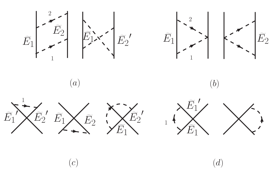
The classes of diagrams contributing to the N3LO box amplitude are illustrated in Fig. 5. The type (a) reducible, and type (c) and (d) irreducible diagrams, are evaluated by keeping next-to-leading (or Q 0Q^{\,0}) terms in the expansions of the energy denominators which include pion energies—see Eq. (8). The amplitude corresponding to the reducible type (b) diagrams is obtained by retaining terms of order QQ in these energy denominators, namely one order higher than for diagrams of type (a), (c), and (d).

We write the N3LO amplitude associated with the box diagrams as the sum of reducible and irreducible contributions, i.e.

T2​π(3)​(ν)=T2​π,red(3)​(ν)+T2​π,irr(3).T_{2\pi}^{(3)}(\nu)=T_{2\pi,\,\rm red}^{(3)}(\nu)+T_{2\pi,\,\rm irr}^{(3)}\ . (74)

The reducible amplitude consists of LS terms plus a term contributing to the definition of the N​NNN potential at N3LO. The latter is affected by the choice of the off-the-energy-shell prescription adopted for the N2LO OPE potential vπ(2)​(ν)v^{(2)}_{\pi}(\nu). As an example, we discuss the results obtained with ν=0\nu=0 and ν=1\nu=1. In particular, for ν=0\nu=0, we find that the box reducible amplitude is given by

T2​π,red(3)​(ν=0)\displaystyle T_{2\pi,\,\rm red}^{(3)}(\nu=0) =\displaystyle= 2​V1​V2ω2​1Ei−E~1−E~2\displaystyle 2\,\frac{V_{1}\,V_{2}}{\omega_{2}}\frac{1}{E_{i}-\widetilde{E}_{1}-\widetilde{E}_{2}} (75)
×\displaystyle\times V3​V4ω13​[(E1−E~1)2+(E2−E~2)2]\displaystyle\frac{V_{3}\,V_{4}}{\omega_{1}^{3}}\left[(E_{1}-\widetilde{E}_{1})^{2}+(E_{2}-\widetilde{E}_{2})^{2}\right]
+\displaystyle+ V1​V2ω23​[(E~1−E1′)2+(E~2−E2′)2]\displaystyle\frac{V_{1}\,V_{2}}{\omega_{2}^{3}}\Big[(\widetilde{E}_{1}-E^{\,\prime}_{1})^{2}+(\widetilde{E}_{2}-E^{\,\prime}_{2})^{2}\Big]
×\displaystyle\times 1Ei−E~1−E~2​ 2​V2​V3ω1\displaystyle\frac{1}{E_{i}-\widetilde{E}_{1}-\widetilde{E}_{2}}\,2\,\frac{V_{2}\,V_{3}}{\omega_{1}}
+\displaystyle+ V1​V2​V3​V4​Ei−E~1−E~2ω12​ω22,\displaystyle\,V_{1}\,V_{2}\,V_{3}\,V_{4}\,\frac{E_{i}-\widetilde{E}_{1}-\widetilde{E}_{2}}{\omega_{1}^{2}\,\omega_{2}^{2}}\ ,

where Ei=E1+E2=E1′+E2′E_{i}=E_{1}+E_{2}=E_{1}^{\prime}+E_{2}^{\prime} is the initial energy of the system, E~j\widetilde{E}_{j} and 𝐪i{\bf q}_{i} (ωi\omega_{i}) denote, respectively, the energies of the intermediate nucleons and momenta (energies) of the exchanged pions as indicated in panels (a) and (b) of Fig. 5, and an integral over an unconstrained pion momentum is understood. In the equation above, and through the remainder of this appendix, we denote with ViV_{i} the vertices entering the diagrams. These vertices are implied by the interaction Hamiltonians listed in Sec. II. For example, the V1V_{1} vertex shown in panel (a) of Fig. 5 is associated with the Hπ​NH_{\pi N} Hamiltonian, and reads

V1=−i​gAFπ​𝝈1⋅𝐪22​ω2​τ1,b,V_{1}=-i\,\frac{g_{A}}{F_{\pi}}\frac{{\bm{\sigma}}_{1}\cdot{\bf q}_{2}}{\sqrt{2\,\omega_{2}}}\tau_{1,b}\ , (76)

where bb specifies the isospin component of the pion.

Refer to caption
Figure 5: Diagrams illustrating the recoil-corrected reducible, panels (a) and (b), and irreducible, panels (c) and (d), amplitudes contributing to the N​NNN potential at N3LO. Pion lines with crossed (full) circle indicate that only the next-to-leading Q 0Q^{\,0} (next-to-next-to-leading Q 1Q^{\,1}) term in the expansion of energy denominators, Eq. (8), are retained in the corresponding amplitudes. See text for explanation. In panels (b), (c), and (d), the crossed or full circles can be either on pion one (as shown in the figure) or on pion two. Only one among the possible time orderings is shown. Notation is as in Fig. 2.

The last term in Eq. (75) is the N3LO recoil-corrected reducible contribution to the N​NNN potential mentioned earlier, corresponding to the prescription ν=0\nu=0. After resolving the spin-isospin structure implied by the vertices, one can easily recognize that the first two terms in T2​π,red(3)T^{(3)}_{2\pi,{\rm red}} represent iterations of the LS equation with the static, vπ(0)v_{\pi}^{(0)}, and N2LO, vπ(2)​(ν=0)v_{\pi}^{(2)}(\nu=0), OPE potentials defined in Eq. (17) and (16), respectively, namely

T2​π,red(3)​(ν=0)\displaystyle T_{2\pi,\,\rm red}^{(3)}(\nu=0)\!\! =\displaystyle= vπ(0)​G0​vπ(2)​(ν=0)+vπ(2)​(ν=0)​G0​vπ(0)\displaystyle\!\!v_{\pi}^{(0)}\,G_{0}\,v_{\pi}^{(2)}(\nu=0)+v_{\pi}^{(2)}(\nu=0)\,G_{0}\,v_{\pi}^{(0)} (77)
+V1​V2​V3​V4​Ei−E~1−E~2ω12​ω22,\displaystyle\!\!+\,V_{1}\,V_{2}\,V_{3}\,V_{4}\,\frac{E_{i}-\widetilde{E}_{1}-\widetilde{E}_{2}}{\omega_{1}^{2}\,\omega_{2}^{2}}\ ,

where, for brevity, the dependence upon nucleon energies and pion momenta is not explicitly indicated. It can be inferred from Fig. 5. If the prescription ν=1\nu=1 is considered for vπ(2)​(ν)v^{(2)}_{\pi}(\nu), the box reducible amplitude at N3LO reads instead

T2​π,red(3)​(ν=1)\displaystyle T_{2\pi,\,\rm red}^{(3)}(\nu=1)\!\! =\displaystyle= vπ(0)​G0​vπ(2)​(ν=1)+vπ(2)​(ν=1)​G0​vπ(0)\displaystyle\!\!v_{\pi}^{(0)}\,G_{0}\,v_{\pi}^{(2)}(\nu=1)+v_{\pi}^{(2)}(\nu=1)\,G_{0}\,v_{\pi}^{(0)} (78)
+V1​V2​V3​V4​[2​ω12+ω22ω13​ω23+1ω12​ω22]\displaystyle\!\!+\,V_{1}\,V_{2}\,V_{3}\,V_{4}\,\left[2\,\frac{\omega_{1}^{2}+\omega_{2}^{2}}{\omega_{1}^{3}\,\omega_{2}^{3}}+\frac{1}{\omega_{1}^{2}\,\omega_{2}^{2}}\right]
×(Ei−E~1−E~2),\displaystyle\!\!\times\left(E_{i}-\widetilde{E}_{1}-\widetilde{E}_{2}\right)\ ,

with vπ(2)​(ν=1)v_{\pi}^{(2)}(\nu=1) as given in Eq. (18), provided the relevant nucleon energies are considered.

Refer to caption
Figure 6: Diagrams illustrating recoil-corrected OPE amplitudes contributing to the charge operator at N3LO. Only one among the possible time orderings is shown. Notation is as in Figs. 2 and 5.

To complete the evaluation of the box amplitude, we need the expression of the irreducible contribution, which is given by

T2​π,irr(3)\displaystyle T_{2\pi,\,\rm irr}^{(3)} =\displaystyle= −V1​V2​V3​V4​Ei−E~1−E~2ω12​ω22\displaystyle-\,V_{1}\,V_{2}\,V_{3}\,V_{4}\,\frac{E_{i}-\widetilde{E}_{1}-\widetilde{E}_{2}}{\omega_{1}^{2}\,\omega_{2}^{2}} (79)
−2V1V4V3V2[E1−E~1+E2′−E~2′ω13​ω2\displaystyle-2\,V_{1}\,V_{4}\,V_{3}\,V_{2}\bigg[\frac{E_{1}-\widetilde{E}_{1}+E_{2}^{\,\prime}-\widetilde{E}^{\,\prime}_{2}}{\omega_{1}^{3}\,\omega_{2}}
+E1′−E~1+E2−E~2′ω1​ω23],\displaystyle+\frac{E_{1}^{\,\prime}-\widetilde{E}_{1}+E_{2}-\widetilde{E}^{\,\prime}_{2}}{\omega_{1}\,\omega_{2}^{3}}\bigg]\ ,

where, referring to Fig. 5, the first term is from the (irreducible) direct diagrams of the type shown in panel (c), while the last two are generated by the diagrams of the type shown in panel (d). The sum of the reducible and irreducible pieces can then be written as

T2​π(3)​(ν)=vπ(0)​G0​vπ(2)​(ν)+vπ(2)​(ν)​G0​vπ(0)+v2​π(3)​(ν),T_{2\pi}^{(3)}(\nu)=v_{\pi}^{(0)}\,G_{0}\,v_{\pi}^{(2)}(\nu)+v_{\pi}^{(2)}(\nu)\,G_{0}\,v_{\pi}^{(0)}+v_{2\pi}^{{(3)}}(\nu)\ , (80)

where v2​π(3)​(ν)v_{2\pi}^{(3)}(\nu) for ν=0,1\nu=0,1 are as given in Eqs. (19) and (20).

An analysis similar to that outlined above leads to the following expressions for the “triangle” TPE, panel (b) of Fig. 4, and OPE contact, panels (c) and (d), amplitudes and corresponding potentials:

T2​π,△(3)=v2​π,△(3)=−gA2Fπ4𝝉1⋅𝝉2∫1ω12​ω22(𝐪1⋅𝐪2\displaystyle\!\!\!\!\!\!\!\!\!\!\!\!\!T^{(3)}_{2\pi,\vartriangle}=v_{2\pi,\vartriangle}^{(3)}=-\frac{g_{A}^{2}}{F_{\pi}^{4}}\,{\bm{\tau}}_{1}\cdot{\bm{\tau}}_{2}\int\frac{1}{\omega_{1}^{2}\,\omega_{2}^{2}}({\bf q}_{1}\cdot{\bf q}_{2}
+i𝝈1⋅𝐪2×𝐪1)(E1+E1′−2E~1)+1⇌2,\displaystyle\qquad\,\!\!\!\!\!\!\!\!\!+\,i\,{\bm{\sigma}}_{1}\cdot{\bf q}_{2}\times{\bf q}_{1})(E_{1}+E_{1}^{\,\prime}-2\,\widetilde{E}_{1})+1\rightleftharpoons 2, (81)
TCT,c(3)​(ν)=vCT(0)​G0​vπ(2)​(ν)+vπ(2)​(ν)​G0​vCT(0)\displaystyle\!\!\!\!\!\!\!\!\!\!\!\!\!\!\!\!\!\!\!\!T_{\rm CT,\,c}^{(3)}(\nu)=v_{\rm CT}^{(0)}\,G_{0}\,v_{\pi}^{(2)}(\nu)+v_{\pi}^{(2)}(\nu)\,G_{0}\,v_{\rm CT}^{(0)}
+vCT,c(3)​(ν),\displaystyle\qquad\,\!\!\!\!\!\!\!\!+\,v_{\rm CT,\,c}^{(3)}(\nu)\ , (82)
TCT,d(3)=vCT,d(3)=3​gA22​Fπ2​∫𝝈1⋅𝐪1​vCT(0)​𝝈1⋅𝐪1ω14\displaystyle\!\!\!\!\!\!\!\!\!\!\!\!\!T_{\rm CT,\,d}^{(3)}=v_{\rm CT,\,d}^{(3)}=\frac{3\,g_{A}^{2}}{2\,F_{\pi}^{2}}\,\,\int\frac{{\bm{\sigma}}_{1}\cdot{\bf q}_{1}\,v_{\rm CT}^{(0)}\,{\bm{\sigma}}_{1}\cdot{\bf q}_{1}}{\omega_{1}^{4}}
×(E1−E~1+E1′−E~1′)+1⇌2,\displaystyle\qquad\,\!\!\!\!\!\!\!\!\times(E_{1}-\widetilde{E}_{1}+E_{1}^{\prime}-\widetilde{E}_{1}^{\prime})+1\rightleftharpoons 2\ , (83)

where

vCT(0)=CS+CT​𝝈1⋅𝝈2,v_{\rm CT}^{(0)}=C_{S}+C_{T}\,{\bm{\sigma}}_{1}\cdot{\bm{\sigma}}_{2}\ , (84)

is the contact potential at LO, while the N3LO potential arising from the diagrams of panel (c) with the choices ν=0,1\nu=0,1 for the OPE potential vπ(2)​(ν)v_{\pi}^{(2)}(\nu), is given by

vCT,c(3)​(ν=0)\displaystyle v_{\rm CT,\,c}^{(3)}(\nu=0)\!\! =\displaystyle= gA22​Fπ2𝝉1⋅𝝉2∫𝝈1⋅𝐪1​vCT(0)​𝝈2⋅𝐪1ω14\displaystyle\!\!\frac{g_{A}^{2}}{2\,F_{\pi}^{2}}\,{\bm{\tau}}_{1}\cdot{\bm{\tau}}_{2}\,\int\frac{{\bm{\sigma}}_{1}\cdot{\bf q}_{1}\,v_{\rm CT}^{(0)}\,{\bm{\sigma}}_{2}\cdot{\bf q}_{1}}{\omega_{1}^{4}} (85)
×\displaystyle\times (E2−E~2+E1′−E~1′)+1⇌2,\displaystyle\!\!(E_{2}-\widetilde{E}_{2}+E_{1}^{\prime}-\widetilde{E}_{1}^{\prime})+1\rightleftharpoons 2\ ,
vCT,c(3)​(ν=1)\displaystyle v_{\rm CT,\,c}^{(3)}(\nu=1)\!\! =\displaystyle= vCT,c(3)​(ν=0)+∫vCT(0)​vπ(0)2​ω12​(Ei−E~1−E~2)\displaystyle\!\!v_{\rm CT,\,c}^{(3)}(\nu=0)+\!\!\int\frac{v_{\rm CT}^{(0)}\,{v_{\pi}^{(0)}}}{2\,\omega_{1}^{2}}(E_{i}-\widetilde{E}_{1}-\widetilde{E}_{2}) (86)
+\displaystyle+ ∫vπ(0)​vCT(0)2​ω12​(Ei−E~1′−E~2′),\displaystyle\int\frac{{v_{\pi}^{(0)}}\,v_{\rm CT}^{(0)}}{2\,\omega_{1}^{2}}(E_{i}-\widetilde{E}_{1}^{\prime}-\widetilde{E}_{2}^{\prime})\ ,

and the nucleon energies and pion momenta are defined in Fig. 4.

B.2 OPE Charge Operators at N3LO

Before turning our attention to the N4LO corrections, we outline the derivation of the N3LO OPE charge operators whose expressions have been given in Eqs. (42)–(44). As discussed in Sec. IV, these operators vanish in the static limit (that is, at N2LO), while at N3LO they are given by amplitudes associated with the diagrams of the type illustrated in Fig. 6. In particular, the charge operator in Eq. (42), which we denote as ργ​π(0)\rho^{(0)}_{\gamma\pi} for later convenience, is obtained as

ργ​π(0)=− 4​V1​V2​Vγ​πω1​ω2​(E1−E1′−E2+E2′).\rho_{\gamma\pi}^{(0)}=-\,4\frac{V_{1}\,V_{2}\,V_{\gamma\pi}}{\omega_{1}\,\omega_{2}}\,(E_{1}-E^{\,\prime}_{1}-E_{2}+E^{\,\prime}_{2})\ . (87)

The vertex Vγ​πV_{\gamma\pi} is proportional to that associated with the interaction Hamiltonian Hγ​πH_{\gamma\pi} in Sec. II,

−i​e​ϵa​b​z​ω1−ω24​ω1​ω2,-i\,e\,\,\epsilon_{abz}\,\,\frac{\omega_{1}-\omega_{2}}{\sqrt{4\,\omega_{1}\,\omega_{2}}}\ , (88)

where the pion energies are as indicated in panel (a) of Fig. 6. It is convenient to factor out the energy numerator (ω1−ω2)(\omega_{1}-\omega_{2}), and define Vγ​πV_{\gamma\pi} as

Vγ​π=−i​e​ϵa​b​z​14​ω1​ω2.V_{\gamma\pi}=-i\,e\,\epsilon_{abz}\,\frac{1}{\sqrt{4\,\omega_{1}\,\omega_{2}}}\ . (89)

Next, we consider the amplitude associated with the diagrams shown in panels (c)–(f) of Fig. 6:

Tγ​d(0)​(ν)\displaystyle T^{(0)}_{\gamma{\rm d}}(\nu) =\displaystyle= [vπ(2)​(ν)​G0​ρ(−3)+ρ(−3)​G0​vπ(2)​(ν)]\displaystyle\left[v_{\pi}^{(2)}(\nu)\,G_{0}\,\rho^{(-3)}+\rho^{(-3)}\,G_{0}\,v_{\pi}^{(2)}(\nu)\right] (90)
+ρd(0)​(ν),\displaystyle+\rho_{\rm d}^{(0)}(\nu)\ ,

where ρ(−3)\rho^{(-3)} is the LO charge operator given in Eq. (36), while ρd(0)​(ν)\rho_{\rm d}^{(0)}(\nu) is the N3LO OPE contribution defined in Eqs. (43)–(44) for ν=0,1\nu=0,1. The latter is written as

ρd(0)​(ν)=ργ​N(0)​(ν)+ρN​γ(0)​(ν)+1⇌2,\rho_{\rm d}^{(0)}(\nu)=\rho_{\gamma N}^{(0)}(\nu)+\rho_{N\gamma}^{(0)}(\nu)+1\rightleftharpoons 2\ , (91)

where ργ​N(0)\rho_{\gamma N}^{(0)} comes from the diagrams shown in panels (c) and (d) of Fig. 6, while ρN​γ(0)\rho_{N\gamma}^{(0)} is associated with those of panels (e) and (f). For ν=0\nu=0, we find

ργ​N(0)​(ν=0)=V1​V2​Vγ​Nω13​(E1′−E¯1+E2−E2′),\displaystyle\!\!\!\!\!\!\!\!\!\!\!\!\!\!\!\!\!\rho_{\gamma N}^{(0)}(\nu=0)=\frac{V_{1}\,V_{2}\,V_{\gamma N}}{\omega_{1}^{3}}\,(E_{1}^{\,\prime}-\overline{E}_{1}+E_{2}-E^{\,\prime}_{2})\ , (92)
ρN​γ(0)​(ν=0)=−VN​γ​V1​V2ω13​(E¯1′−E1+E2−E2′),\displaystyle\!\!\!\!\!\!\!\!\!\!\!\!\!\!\!\!\!\rho_{N\gamma}^{(0)}(\nu=0)=-\frac{V_{N\gamma}\,V_{1}\,V_{2}}{\omega_{1}^{3}}(\overline{E}_{1}^{\,\prime}-E_{1}+E_{2}-E^{\,\prime}_{2})\ , (93)

while for ν=1\nu=1 we obtain

ργ​N(0)​(ν=1)\displaystyle\rho_{\gamma N}^{(0)}(\nu=1) =\displaystyle= 2​V1​V2​Vγ​Nω13​(E2−E2′),\displaystyle 2\,\frac{V_{1}\,V_{2}\,V_{\gamma N}}{\omega_{1}^{3}}\,(E_{2}-E^{\,\prime}_{2})\ , (94)
ρN​γ(0)​(ν=1)\displaystyle\rho_{N\gamma}^{(0)}(\nu=1) =\displaystyle= −2​Vγ​N​V1​V2ω13​(E2−E2′).\displaystyle-2\,\frac{V_{\gamma N}\,V_{1}\,V_{2}}{\omega_{1}^{3}}\,(E_{2}-E^{\,\prime}_{2})\ . (95)

The energies E¯1\overline{E}_{1} and E¯1′\overline{E}_{1}^{\,\prime} are as indicated in panels (c) and (e) of Fig. 6, respectively, and Vγ​N=e​eN,1V_{\gamma N}=e\,e_{N,1} is the vertex implied by the interaction Hamiltonian Hγ​NH_{\gamma N} at LO.

B.3 N4LO Charge Operators

Refer to caption

Figure 7: Diagrams illustrating the static, panels (d), (e), (i), and (j), and recoil-corrected, remaining panels, diagrams associated with the N4LO contribution shown in panel (c) of Fig. 3. Only one among the possible time orderings is shown. Notation is as in Figs. 2 and 5.

We can now proceed to sketch the derivation of the charge operators illustrated in panels (c)–(j) of Fig. 3. The one-loop corrections of panels (c)–(e) involve a γ​π​π{\gamma\pi\pi} electromagnetic vertex, while a γ​N​N\gamma NN interaction enters those of panels (f)–(j). We give details on the derivation of the operators ρc(1)\rho^{(1)}_{\rm c} and ρh(1)\rho^{(1)}_{\rm h} as representatives of these classes of diagrams.

First, we consider the pion-in-flight term. The diagrams contributing at N4LO are shown in Fig. 7. As diagrammatically shown in the figure, the irreducible contributions, panels (d), (e), (i), and (j), are evaluated in the static limit, while next-to-leading order terms in the expansion of energy denominators are retained in the evaluation of the reducible contributions. We write the total amplitude as a sum of these, that is

Tγ​c(1)\displaystyle T_{\gamma{\rm c}}^{(1)} =\displaystyle= Tγ​c,red(1)+Tγ​c,irr(1).\displaystyle T_{\gamma{\rm c,\,red}}^{(1)}+T_{\gamma{\rm c,\,irr}}^{(1)}\ . (96)

The reducible and irreducible contributions are given by

Tγ​c,red(1)\displaystyle\!\!\!\!\!\!\!\!\!\!T_{\gamma{\rm c,\,red}}^{(1)}\!\! =\displaystyle= vπ(0)​G0​ργ​π(0)+ργ​π(0)​G0​vπ(0)\displaystyle\!\!v_{\pi}^{(0)}\,G_{0}\,\rho_{\gamma\pi}^{(0)}+\rho_{\gamma\pi}^{(0)}\,G_{0}\,v_{\pi}^{(0)} (97)
+\displaystyle+ 2​(ω1−ω3)ω1​ω2​ω3​(ω1+ω3)​[V1​V2,V3​V4]​Vγ​π,\displaystyle\!\!\frac{2\,(\omega_{1}-\omega_{3})}{\omega_{1}\,\omega_{2}\,\omega_{3}\,(\omega_{1}+\omega_{3})}\,\left[V_{1}\,V_{2}\,,\,V_{3}\,V_{4}\right]V_{\gamma\pi}\ ,
Tγ​c,irr(1)\displaystyle\!\!\!\!\!\!\!\!\!\!T_{\gamma{\rm c,\,irr}}^{(1)}\!\! =\displaystyle= −2​(ω1−ω3)ω1​ω2​ω3​(ω1+ω3)​[V1​V2,V3​V4]​Vγ​π\displaystyle\!\!-\frac{2\,(\omega_{1}-\omega_{3})}{\omega_{1}\,\omega_{2}\,\omega_{3}\,(\omega_{1}+\omega_{3})}\left[V_{1}\,V_{2}\,,\,V_{3}\,V_{4}\right]V_{\gamma\pi} (98)
−\displaystyle- 8ω1​ω2​ω3​[V1​V4,V3​V2]​Vγ​π,\displaystyle\!\!\frac{8}{\omega_{1}\,\omega_{2}\,\omega_{3}}\,\left[V_{1}\,V_{4}\,,\,V_{3}\,V_{2}\right]V_{\gamma\pi}\ ,

where […,…][\dots,\dots] denotes a commutator and ργ​π(0)\rho_{\gamma\pi}^{(0)} is the N3LO OPE charge operator defined in Eq. (87). In Eq. (97), the terms multiplied by the spin-isospin combinations V1​V2​V3​V4​Vγ​πV_{1}\,V_{2}\,V_{3}\,V_{4}\,V_{\gamma\pi} and V3​V4​V1​V2​Vγ​πV_{3}\,V_{4}\,V_{1}\,V_{2}\,V_{\gamma\pi} come from the diagrams shown in panels (a)–(c) and (f)–(h), respectively, whereas in Eq. (98) the first term results from the evaluation of the diagrams shown in panels (d) and (i) of Fig. 7 and the second one is from those illustrated in panels (e) and (j). The total amplitude is then given by

Tγ​c(1)\displaystyle T_{\gamma{\rm c}}^{(1)} =\displaystyle= vπ(0)​G0​ργ​π(0)+ργ​π(0)​G0​vπ(0)+ρc(1),\displaystyle v_{\pi}^{(0)}\,G_{0}\,\rho_{\gamma\pi}^{(0)}+\rho_{\gamma\pi}^{(0)}\,G_{0}\,v_{\pi}^{(0)}+\rho_{\rm c}^{(1)}\ , (99)

where

ρc(1)=−8ω1​ω2​ω3​[V1​V4,V3​V2]​Vγ​π,\rho^{(1)}_{\rm c}=-\frac{8}{\omega_{1}\,\omega_{2}\,\omega_{3}}\,\left[V_{1}\,V_{4}\,,\,V_{3}\,V_{2}\right]\,V_{\gamma\pi}\ , (100)

which, after resolving the spin-isospin structure implied by the vertices, reduces to the N4LO charge operator in Eq. (47).

We now turn our attention to the one-loop correction shown in panel (h) of Fig. 3. For this contribution, we distinguish among three classes of diagrams depending on whether the photon is absorbed before pion one, class A, after pion one, class B, or after pion two, class C. These classes are represented in Fig. 8—the vertices and kinetic energies of intermediate nucleons are as indicated in the figure.

We start off by discussing the result obtained for the class A amplitude. In Fig. 9 we show the diagrams contributing at N4LO. The irreducible diagrams, panels (f) and (g) of this figure, are evaluated in the static limit. The N4LO recoil-corrected contributions associated with the single (double) reducible diagrams, panels (c)–(e) of Fig. 9 [panels (a) and (b)], are obtained by retaining Q 0Q^{\,0} (Q 1Q^{\,1}) terms in the expansions of energy denominators involving pions. The N4LO amplitude is then written as

Tγ​A(1)​(ν)\displaystyle T_{\gamma{\rm A}}^{(1)}(\nu) =\displaystyle= Tγ​A,red(1)​(ν)+Tγ​A,irr,\displaystyle T_{\gamma{\rm A,\,red}}^{(1)}(\nu)+T_{\gamma{\rm A,\,irr}}\ , (101)

where

Tγ​A,red(1)​(ν=0)\displaystyle T_{\gamma{\rm A,\,red}}^{(1)}(\nu=0)\!\! =\displaystyle= [vπ(0)G0vπ(2)(ν=0)G0ρ(−3)\displaystyle\!\!\bigg[v_{\pi}^{(0)}\,G_{0}\,v_{\pi}^{(2)}(\nu=0)\,G_{0}\,\rho^{(-3)} (102)
+vπ(2)​(ν=0)​G0​vπ(0)​G0​ρ(−3)\displaystyle\!\!\!\!\!\!\!\!\!\!\!\!\!\!\!\!\!\!\!\!\!\!\!\!\!\!+\,v_{\pi}^{(2)}(\nu=0)\,G_{0}\,v_{\pi}^{(0)}\,G_{0}\,\rho^{(-3)}
+v2​π(3)(ν=0)G0ρ(−3)+vπ(0)G0ργ​N(0)(ν=0)]\displaystyle\!\!\!\!\!\!\!\!\!\!\!\!\!\!\!\!\!\!\!\!\!\!\!\!\!\!+\,v_{2\pi}^{{(3)}}(\nu=0)\,G_{0}\,\rho^{(-3)}+v_{\pi}^{(0)}\,G_{0}\,\rho_{\gamma N}^{(0)}(\nu=0)\bigg]
+[2ω13​ω2−1ω1​ω2​(ω1+ω2)2−1ω12​ω2​(ω1+ω2)]\displaystyle\!\!\!\!\!\!\!\!\!\!\!\!\!\!\!\!\!\!\!\!\!\!\!\!\!\!+\,\bigg[\frac{2}{\omega_{1}^{3}\,\omega_{2}}-\frac{1}{\omega_{1}\,\omega_{2}(\omega_{1}+\omega_{2})^{2}}-\frac{1}{\omega_{1}^{2}\,\omega_{2}(\omega_{1}+\omega_{2})}\bigg]
×V1​V2​V3​V4​Vγ​N\displaystyle\!\!\!\!\!\!\!\!\!\!\!\!\!\!\!\!\!\!\!\!\!\!\!\!\!\!\times\,V_{1}\,V_{2}\,V_{3}\,V_{4}\,V_{\gamma N}
+[1ω1​ω2​(ω1+ω2)2−2ω13​ω2−2ω1​ω23]\displaystyle\!\!\!\!\!\!\!\!\!\!\!\!\!\!\!\!\!\!\!\!\!\!\!\!\!\!+\bigg[\frac{1}{\omega_{1}\,\omega_{2}\,(\omega_{1}+\omega_{2})^{2}}-\frac{2}{\omega_{1}^{3}\,\omega_{2}}-\frac{2}{\omega_{1}\,\omega_{2}^{3}}\bigg]
×V1​V4​V3​V2​Vγ​N+1⇌2.\displaystyle\!\!\!\!\!\!\!\!\!\!\!\!\!\!\!\!\!\!\!\!\!\!\!\!\!\!\times\,V_{1}\,V_{4}\,V_{3}\,V_{2}\,V_{\gamma N}+1\rightleftharpoons 2\ .

The N4LO LS terms arising from the reducible diagrams are listed in the first two lines of the equation above, where vπ(0)v_{\pi}^{(0)}, vπ(2)​(ν=0)v_{\pi}^{(2)}(\nu=0) and v2​π(3)​(ν=0)v_{2\pi}^{(3)}(\nu=0) are the LO, N2LO and N3LO components of the N​NNN potential given in Eqs. (17), (16), and (19), respectively, while the ρ(−3)\rho^{(-3)} and ργ​N(0)\rho_{\gamma N}^{(0)} charge operators have been defined in Eqs. (36) and (92). The last two terms in Eq. (102) constitute the N4LO recoil-corrected contribution associated with the reducible diagrams. In particular, the second term is generated by the direct reducible diagrams of panels (a)–(c) and (e), while the last one is obtained from the contributions of type (d).

Refer to caption

Figure 8: Classes of diagrams associated with the one-loop contribution illustrated in panel (h) of Fig. 3. Notation is as in Fig. 2.

The irreducible amplitude from diagrams in panels (f) and (g) of Fig. 9 reads

Tγ​A,irr(1)\displaystyle T_{\gamma{\rm A,\,irr}}^{(1)} =\displaystyle= [1ω1​ω2​(ω1+ω2)2+1ω12​ω2​(ω1+ω2)]\displaystyle\left[\frac{1}{\omega_{1}\,\omega_{2}(\omega_{1}+\omega_{2})^{2}}+\frac{1}{\omega_{1}^{2}\,\omega_{2}\,(\omega_{1}+\omega_{2})}\right] (103)
×\displaystyle\times V1​V2​V3​V4​Vγ​N\displaystyle V_{1}\,V_{2}\,V_{3}\,V_{4}\,V_{\gamma N}
+\displaystyle+ [2ω1​ω23−1ω1​ω2​(ω1+ω2)2]\displaystyle\left[\frac{2}{\omega_{1}\,\omega_{2}^{3}}-\frac{1}{\omega_{1}\,\omega_{2}(\omega_{1}+\omega_{2})^{2}}\right]
×\displaystyle\times V1​V4​V3​V2​Vγ​N+1⇌2,\displaystyle V_{1}\,V_{4}\,V_{3}\,V_{2}\,V_{\gamma N}+1\rightleftharpoons 2\ ,

and combining Eqs. (102) and (103) leads to a total amplitude, which can be written as

Tγ​A(1)​(ν)\displaystyle T_{\gamma{\rm A}}^{(1)}(\nu) =\displaystyle= vπ(0)​G0​vπ(2)​(ν)​G0​ρ(−3)\displaystyle v_{\pi}^{(0)}\,G_{0}\,v_{\pi}^{(2)}(\nu)\,G_{0}\,\rho^{(-3)} (104)
+\displaystyle+ vπ(2)​(ν)​G0​vπ(0)​G0​ρ(−3)+v2​π(3)​(ν)​G0​ρ(−3)\displaystyle v_{\pi}^{(2)}(\nu)\,G_{0}\,v_{\pi}^{(0)}\,G_{0}\,\rho^{(-3)}+v_{2\pi}^{{(3)}}(\nu)\,G_{0}\,\rho^{(-3)}
+\displaystyle+ vπ(0)​G0​ργ​N(0)​(ν)+ρA(1)​(ν)+1⇌2,\displaystyle v_{\pi}^{(0)}\,G_{0}\,\rho_{\gamma N}^{(0)}(\nu)+\rho_{\rm A}^{(1)}(\nu)+1\rightleftharpoons 2\ ,

where

ρA(1)​(ν=0)=2ω13​ω2​V1​V3​[V2,V4]​Vγ​N.\rho_{\rm A}^{(1)}(\nu=0)=\frac{2}{\omega_{1}^{3}\,\omega_{2}}\,V_{1}\,V_{3}\,\left[V_{2}\,,\,V_{4}\right]\,V_{\gamma N}\ . (105)

Refer to caption

Figure 9: Diagrams illustrating the static, panels (f) and (g), and recoil-corrected, remaining panels, class A diagrams contributing at N4LO. In panels (b)–(e), the crossed and full circles can be either on pion one (as shown in the figure) or on pion two. Only one among the possible time orderings is shown. Notation is as in Figs. 2 and 5.

The derivation of the class C amplitude (see Fig. 8) is analogous to that described above. We find:

Tγ​C(1)​(ν)\displaystyle\!\!\!\!\!\!\!\!T_{\gamma{\rm C}}^{(1)}(\nu) =\displaystyle= ρ(−3)​G0​vπ(0)​G0​vπ(2)​(ν)\displaystyle\rho^{(-3)}\,G_{0}\,v_{\pi}^{(0)}\,G_{0}\,v_{\pi}^{(2)}(\nu) (106)
+\displaystyle+ ρ(−3)​G0​vπ(2)​(ν)​G0​vπ(0)+ρ(−3)​G0​v2​π(3)​(ν)\displaystyle\rho^{(-3)}\,G_{0}\,v_{\pi}^{(2)}(\nu)\,G_{0}\,v_{\pi}^{(0)}+\rho^{(-3)}\,G_{0}\,v_{2\pi}^{{(3)}}(\nu)
+\displaystyle+ ρN​γ(0)​(ν)​G0​vπ(0)+ρC(1)​(ν)+1⇌2,\displaystyle\rho_{N\gamma}^{(0)}(\nu)\,G_{0}\,v_{\pi}^{(0)}+\rho_{\rm C}^{(1)}(\nu)+1\rightleftharpoons 2\ ,

where ρN​γ(0)\rho_{N\gamma}^{(0)} is the OPE charge operator defined in Eq. (93), and

ρC(1)​(ν=0)\displaystyle\rho_{\rm C}^{(1)}(\nu=0) =\displaystyle= 2ω1​ω23​Vγ​N​V1​V3​[V2,V4].\displaystyle\frac{2}{\omega_{1}\,\omega_{2}^{3}}\,\,V_{\gamma N}V_{1}\,V_{3}\,\left[V_{2}\,,\,V_{4}\right]\ . (107)

Class B of box diagrams at N4LO are shown in Fig. 10. The reducible amplitude, associated with the diagrams in panels (a)–(d), is found to be

Tγ​B,red(1)​(ν=0)\displaystyle T_{\,\gamma{\rm B,\,red}}^{(1)}(\nu=0)\!\!\! =\displaystyle= vπ(0)​G0​ρ(−3)​G0​vπ(2)​(ν=0)\displaystyle\!\!v_{\pi}^{(0)}\,G_{0}\,\rho^{(-3)}\,G_{0}\,v_{\pi}^{(2)}(\nu=0) (108)
+vπ(2)​(ν=0)​G0​ρ(−3)​G0​vπ(0)\displaystyle\!\!\!\!\!\!\!\!\!\!\!\!\!\!\!\!\!\!\!\!\!\!\!\!\!\!\!\!\!\!\!\!\!\!\!\!\!\!\!\!\!+\,v_{\pi}^{(2)}(\nu=0)\,G_{0}\,\rho^{(-3)}\,G_{0}\,v_{\pi}^{(0)}
+ργ​N(0)​(ν=0)​G0​vπ(0)+vπ(0)​G0​ρN​γ(0)​(ν=0)\displaystyle\!\!\!\!\!\!\!\!\!\!\!\!\!\!\!\!\!\!\!\!\!\!\!\!\!\!\!\!\!\!\!\!\!\!\!\!\!\!\!\!\!+\rho_{\gamma N}^{(0)}(\nu=0)\,G_{0}\,v_{\pi}^{(0)}+v_{\pi}^{(0)}\,G_{0}\,\rho_{N\gamma}^{(0)}(\nu=0)
−(2​ω12+ω22ω13​ω23+1ω12​ω22)​V1​V2​Vγ​N​V3​V4+1⇌2,\displaystyle\!\!\!\!\!\!\!\!\!\!\!\!\!\!\!\!\!\!\!\!\!\!\!\!\!\!\!\!\!\!\!\!\!\!\!\!\!\!\!\!\!-\bigg(2\,\frac{\omega_{1}^{2}+\omega_{2}^{2}}{\omega_{1}^{3}\,\omega_{2}^{3}}+\frac{1}{\omega_{1}^{2}\,\omega_{2}^{2}}\bigg)V_{1}V_{2}V_{\gamma N}V_{3}V_{4}\!+\!1\rightleftharpoons 2\ ,

while the irreducible amplitude, corresponding to the diagrams in panels (e) and (f), amounts to

Tγ​B,irr(1)\displaystyle T_{\gamma{\rm B,\,irr}}^{(1)}\!\! =\displaystyle= 1ω12​ω22​V1​V2​Vγ​N​V3​V4\displaystyle\!\!\frac{1}{\omega_{1}^{2}\,\omega_{2}^{2}}\,V_{1}\,V_{2}\,V_{\gamma N}\,V_{3}\,V_{4} (109)
+\displaystyle+ 2​ω12+ω22ω13​ω23​V1​V4​Vγ​N​V3​V2+1⇌2,\displaystyle\!\!2\,\frac{\omega_{1}^{2}+\omega_{2}^{2}}{\omega_{1}^{3}\,\omega_{2}^{3}}\,V_{1}\,V_{4}\,V_{\gamma N}\,V_{3}\,V_{2}+1\rightleftharpoons 2\ ,

and the class B amplitude is then given by

Tγ​B(1)​(ν)\displaystyle T_{\gamma{\rm B}}^{(1)}(\nu) =\displaystyle= vπ(0)​G0​ρ(−3)​G0​vπ(2)​(ν)\displaystyle v_{\pi}^{(0)}\,G_{0}\,\rho^{(-3)}\,G_{0}\,v_{\pi}^{(2)}(\nu) (110)
+\displaystyle+ vπ(2)​(ν)​G0​ρ(−3)​G0​vπ(0)\displaystyle v_{\pi}^{(2)}(\nu)\,G_{0}\,\rho^{(-3)}\,G_{0}\,v_{\pi}^{(0)}
+\displaystyle+ ργ​N(0)​(ν)​G0​vπ(0)+vπ(0)​G0​ρN​γ(0)​(ν)\displaystyle\rho_{\gamma N}^{(0)}(\nu)\,G_{0}\,v_{\pi}^{(0)}+v_{\pi}^{(0)}\,G_{0}\,\rho_{N\gamma}^{(0)}(\nu)
+\displaystyle+ ρB(1)​(ν)+1⇌2,\displaystyle\rho_{\rm B}^{(1)}(\nu)+1\rightleftharpoons 2\ ,

where

ρB(1)​(ν=0)=− 2​ω12+ω22ω13​ω23​V1​Vγ​N​V3​[V4,V2].\rho_{\rm B}^{(1)}(\nu=0)=\,-\,2\,\frac{\omega_{1}^{2}+\omega_{2}^{2}}{\omega_{1}^{3}\,\omega_{2}^{3}}\,\,V_{1}\,V_{\gamma N}\,V_{3}\,\left[V_{4}\,,\,V_{2}\right]\ . (111)

Finally, the total amplitude associated with the diagram shown in panel (h) of Fig. 3 is given by the sum of the A, B, and C amplitudes, that is

Th(1)​(ν)\displaystyle T_{\rm h}^{(1)}(\nu) =\displaystyle= Tγ​A(1)​(ν)+Tγ​B(1)​(ν)+Tγ​C(1)​(ν)\displaystyle T_{\gamma{\rm A}}^{(1)}(\nu)+T_{\gamma{\rm B}}^{(1)}(\nu)+T_{\gamma{\rm C}}^{(1)}(\nu) (112)
=\displaystyle= [[ρ(−3)G0vπ(0)G0vπ(2)(ν)+permutations]\displaystyle\bigg[\left[\rho^{(-3)}\,G_{0}\,v_{\pi}^{(0)}\,G_{0}\,v_{\pi}^{(2)}(\nu)+{\rm permutations}\right]
+\displaystyle+ [ρ(−3)G0v2​π(3)(ν)+v2​π(3)(ν)G0ρ(−3)]+1⇌2]\displaystyle\left[\rho^{(-3)}\,G_{0}\,v_{2\pi}^{{(3)}}(\nu)+v_{2\pi}^{{(3)}}(\nu)\,G_{0}\,\rho^{(-3)}\right]+1\rightleftharpoons 2\bigg]
+\displaystyle+ [ρd(0)​(ν)​G0​vπ(0)+vπ(0)​G0​ρd(0)​(ν)]\displaystyle\left[\rho_{\rm d}^{(0)}(\nu)\,G_{0}\,v_{\pi}^{(0)}+v_{\pi}^{(0)}\,G_{0}\,\rho_{\rm d}^{(0)}(\nu)\right]
+\displaystyle+ ρh(1)​(ν),\displaystyle\rho_{\rm h}^{(1)}(\nu),

where ρd(0)\rho_{\rm d}^{(0)} is defined as in Eq. (91), while

ρh(1)​(ν)=ρA(1)​(ν)+ρB(1)​(ν)+ρC(1)​(ν)+1⇌2.\displaystyle\rho_{\rm h}^{(1)}(\nu)=\rho_{\rm A}^{(1)}(\nu)+\rho_{\rm B}^{(1)}(\nu)+\rho_{\rm C}^{(1)}(\nu)+1\rightleftharpoons 2\ . (113)

For ν=0\nu=0, ρA(1)\rho_{\rm A}^{(1)}, ρB(1)\rho_{\rm B}^{(1)}, and ρC(1)\rho_{\rm C}^{(1)} are as given in Eqs. (105),  (111), and (107), respectively, and carrying out the spin-isospin algebra leads to Eq. (50). Similarly, for ν=1\nu=1 we find:

ρA(1)​(ν=1)=ρA(1)​(ν=0)+2ω1​ω23​V1​V2​V3​V4​Vγ​N,\displaystyle\!\!\!\!\!\!\!\!\!\!\!\!\!\!\!\!\!\!\!\!\!\!\rho_{\rm A}^{(1)}(\nu=1)=\rho_{\rm A}^{(1)}(\nu=0)+\frac{2}{\omega_{1}\,\omega_{2}^{3}}\,V_{1}\,V_{2}\,V_{3}\,V_{4}\,V_{\gamma N}\ , (114)
ρB(1)​(ν=1)=ρB(1)​(ν=0),\displaystyle\!\!\!\!\!\!\!\!\!\!\!\!\!\!\!\!\!\!\!\!\!\!\rho_{\rm B}^{(1)}(\nu=1)=\rho_{\rm B}^{(1)}(\nu=0)\ , (115)
ρC(1)​(ν=1)=ρC(1)​(ν=0)−2ω1​ω23​Vγ​N​V1​V2​V3​V4,\displaystyle\!\!\!\!\!\!\!\!\!\!\!\!\!\!\!\!\!\!\!\!\!\!\rho_{\rm C}^{(1)}(\nu=1)=\rho_{\rm C}^{(1)}(\nu=0)-\frac{2}{\omega_{1}\,\omega_{2}^{3}}\,V_{\gamma N}\,V_{1}\,V_{2}\,V_{3}\,V_{4}\ , (116)

from which it follows that

ρh​(ν=1)\displaystyle\hskip-23.84923pt\rho_{\rm h}(\nu=1)\!\! =\displaystyle= ρh​(ν=0)\displaystyle\!\!\rho_{\rm h}(\nu=0) (117)
+\displaystyle+ [2ω1​ω23[V1V2V3V4,Vγ​N]+1⇌2],\displaystyle\!\!\left[\frac{2}{\omega_{1}\,\omega_{2}^{3}}\,[V_{1}\,V_{2}\,V_{3}\,V_{4}\,,\,V_{\gamma N}]+1\rightleftharpoons 2\right]\ ,

and simplifying the spin-isospin structures leads to the operator ρh(1)​(ν=1)\rho^{(1)}_{\rm h}(\nu=1) given in Eq. (51).

Below we list the expressions for the amplitudes associated with the remaining N4LO one-loop corrections illustrated in Fig. 3, in particular, referring to panels (d), (e), (g), (i), and (j) of this figure (type (f) operator vanishes as pointed out in Sec. V) we obtain:

Td(1)\displaystyle\!\!\!\!\!\!\!\!\!\!\!\!\!\!\!\!\!\!T_{\rm d}^{(1)}\!\!\! =\displaystyle= [vCT(0)​G0​ργ​π(0)+ργ​π(0)​G0​vCT(0)],\displaystyle\!\!\!\left[v_{\rm CT}^{(0)}\,G_{0}\,\rho_{\gamma\pi}^{(0)}+\rho_{\gamma\pi}^{(0)}\,G_{0}\,v_{\rm CT}^{(0)}\right]\ , (118)
Te(1)\displaystyle T_{\rm e}^{(1)}\!\!\! =\displaystyle= ρe(1),\displaystyle\!\!\!\rho_{\rm e}^{(1)}\ , (119)
Tg(1)\displaystyle T_{\rm g}^{(1)}\!\!\! =\displaystyle= [v2​π,△(3)G0ρ(−3)+ρ(−3)G0v2​π,△(3)+1⇌2]\displaystyle\!\!\!\left[v_{2\pi,\vartriangle}^{(3)}\,G_{0}\,\rho^{(-3)}+\rho^{(-3)}\,G_{0}\,v_{2\pi,\vartriangle}^{(3)}+1\rightleftharpoons 2\right] (120)
+\displaystyle+ ρg(1),\displaystyle\!\!\!\rho_{\rm g}^{(1)}\ ,
Ti(1)​(ν)\displaystyle T_{\rm i}^{(1)}(\nu)\!\!\! =\displaystyle= [[ρ(−3)G0vCT(0)G0vπ(2)(ν)+permutations]\displaystyle\!\!\!\bigg[\!\left[\rho^{(-3)}\,G_{0}\,v_{\rm CT}^{(0)}\,G_{0}\,v_{\pi}^{(2)}(\nu)+{\rm permutations}\right] (121)
+\displaystyle+ [ρ(−3)G0vCT,c(3)(ν)+vCT,c(3)(ν)G0ρ(−3)]+1⇌2]\displaystyle\!\!\!\big[\rho^{(-3)}\,G_{0}\,v_{\rm CT,\,c}^{{(3)}}(\nu)+v_{\rm CT,\,c}^{{(3)}}(\nu)\,G_{0}\,\rho^{(-3)}\big]+1\rightleftharpoons 2\bigg]
+\displaystyle+ [ρd(0)​(ν)​G0​vCT(0)+vCT(0)​G0​ρd(0)​(ν)]\displaystyle\!\!\!\left[\rho_{\rm d}^{(0)}(\nu)\,G_{0}\,v_{\rm CT}^{(0)}+v_{\rm CT}^{(0)}\,G_{0}\,\rho_{\rm d}^{(0)}(\nu)\right]
+\displaystyle+ ρi(1)​(ν),\displaystyle\!\!\!\rho_{\rm i}^{(1)}(\nu)\ ,
Tj(1)\displaystyle T_{\rm j}^{(1)}\!\!\! =\displaystyle= [vCT,d(3)G0ρ(−3)+ρ(−3)G0vCT,d(3)+1⇌2]\displaystyle\!\!\!\left[v_{\rm CT,\,d}^{(3)}\,G_{0}\,\rho^{(-3)}+\rho^{(-3)}\,G_{0}\,v_{\rm CT,\,d}^{(3)}+1\rightleftharpoons 2\right] (122)
+\displaystyle+ ρj(1),\displaystyle\!\!\!\rho_{\rm j}^{(1)}\ ,

where ρe(1)\rho_{\rm e}^{(1)}, ρg(1)\rho_{\rm g}^{(1)}, and ρj(1)\rho_{\rm j}^{(1)} are given in Eqs. (48),  (49), and (53), respectively, while ρi(1)\rho_{\rm i}^{(1)} with ν=0,1\nu=0,1 vanishes. In the equations above the LS terms involve the LO contact, Eq. (84), and N2LO OPE components of the N​NNN potential, Eqs. (16) and  (18), as well as the N3LO potential v(3)v^{(3)}, derived in Sec. B.1. In addition, the ρ(−3)\rho^{(-3)} is defined in Eq. (36), while the N3LO OPE charge operators, ρ(0)\rho^{(0)}, are listed in Sec. B.2.

Refer to caption

Figure 10: Diagrams illustrating the static, panels (e) and (f), and recoil-corrected, remaining panels, class B diagrams contributing at N4LO. In panels (b)–(d), the crossed and full circles can be either on pion one (as shown in the figure) or on pion two. Only one among the possible time orderings is shown. Notation is as in Figs. 2 and 5.

Appendix C The N4LO charge operators in rr-space

The configuration-space representations of the charge operators at order n=−3,…,0n=-3,\dots,0 are well known [18]. Here we obtain those corresponding to ρ(1)\rho^{(1)} for ν=0\nu=0 only. Note that ρa(1)\rho^{(1)}_{\rm a}, ρd(1)\rho^{(1)}_{\rm d}, and ρi(1)​(ν=0)\rho^{(1)}_{\rm i}(\nu=0) vanish. Next, consider

ρb(1)​(𝐪)\displaystyle\rho^{(1)}_{\rm b}({\bf q})\!\! =\displaystyle=\!\! e​2​gA2Fπ4​τ2,z​∫𝐤1,𝐤2ei​𝐤1⋅𝐫1​ei​𝐤2⋅𝐫2​δ¯​(𝐤1+𝐤2−𝐪)\displaystyle\!\!e\,\frac{2\,g_{A}^{2}}{F_{\pi}^{4}}\,\tau_{2,z}\!\!\int_{{\bf k}_{1},{\bf k}_{2}}\!\!{\rm e}^{i{\bf k}_{1}\cdot{\bf r}_{1}}\,{\rm e}^{i{\bf k}_{2}\cdot{\bf r}_{2}}\,\overline{\delta}({\bf k}_{1}\!+\!{\bf k}_{2}\!-{\bf q}) (123)
×\displaystyle\times ∫𝐪1,𝐪2𝐪1⋅𝐪2ω12​ω22​δ¯​(𝐪1+𝐪2−𝐤1)+1⇌2\displaystyle\int_{{\bf q}_{1},{\bf q}_{2}}\!\!\frac{{\bf q}_{1}\cdot{\bf q}_{2}}{\omega_{1}^{2}\,\omega_{2}^{2}}\,\overline{\delta}({\bf q}_{1}\!+\!{\bf q}_{2}\!-\!{\bf k}_{1})\,+1\rightleftharpoons 2
=\displaystyle= −e2​gA2Fπ4τ2,zei​𝐪⋅𝐫2[∇fπ(r)]⋅[∇fπ(r)]\displaystyle\!\!-e\,\frac{2\,g_{A}^{2}}{F_{\pi}^{4}}\,\tau_{2,z}\,{\rm e}^{i{\bf q}\cdot{\bf r}_{2}}\left[{\bm{\nabla}}f_{\pi}(r)\right]\cdot\left[{\bm{\nabla}}f_{\pi}(r)\right]
+\displaystyle+ 1⇌2,\displaystyle 1\rightleftharpoons 2\ ,

where in the second line 𝐫{\bf r} denotes the relative position 𝐫=𝐫1−𝐫2{\bf r}={\bf r}_{1}-{\bf r}_{2} of the two nucleons, and

fπ​(r)=∫𝐩ei​𝐩⋅𝐫​1p2+mπ2=14​π​e−mπ​rr.f_{\pi}(r)=\int_{\bf p}{\rm e}^{i{\bf p}\cdot{\bf r}}\,\frac{1}{p^{2}+m_{\pi}^{2}}=\frac{1}{4\pi}\frac{{\rm e}^{-m_{\pi}r}}{r}\ . (124)

Of course, the expression above is ill-behaved in the limit of vanishing internucleon separations, and needs to be regularized. This can be accomplished by replacing

fπ​(r)→fΛ​(r)=∫𝐩ei​𝐩⋅𝐫​CΛ​(p)p2+mπ2,f_{\pi}(r)\rightarrow f_{\Lambda}(r)=\int_{\bf p}{\rm e}^{i{\bf p}\cdot{\bf r}}\,\frac{C_{\Lambda}(p)}{p^{2}+m_{\pi}^{2}}\ , (125)

and in applications so far [22] the cutoff function has been taken as CΛ(p)=exp(−p4/Λ4)C_{\Lambda}(p)={\rm exp}(-p^{4}/\Lambda^{4}). Similarly, we find:

ρc(1)\displaystyle\rho^{(1)}_{\rm c}\!\! =\displaystyle= −e2​gA4Fπ4[2(τ1,z+τ2,z)\displaystyle\!\!\!-e\,\frac{2\,g_{A}^{4}}{F_{\pi}^{4}}\Big[2\,(\tau_{1,z}+\tau_{2,z}) (126)
×\displaystyle\times [ϵα​β​γ​ϵλ​μ​ν​σ1,α​σ2,λ+δβ​γ​δμ​ν]\displaystyle\!\!\!\big[\epsilon_{\alpha\beta\gamma}\epsilon_{\lambda\mu\nu}\,\sigma_{1,\alpha}\,\sigma_{2,\lambda}+\delta_{\beta\gamma}\delta_{\mu\nu}\big]
−\displaystyle- (𝝉1×𝝉2)z[δβ​γϵλ​μ​νσ2,λ−ϵα​β​γδμ​νσ1,α]]\displaystyle\!\!\!({\bm{\tau}}_{1}\times{\bm{\tau}}_{2})_{z}\,\big[\delta_{\beta\gamma}\,\epsilon_{\lambda\mu\nu}\,\sigma_{2,\lambda}-\epsilon_{\alpha\beta\gamma}\,\delta_{\mu\nu}\,\sigma_{1,\alpha}\big]\Big]
×\displaystyle\times [∂1,β∂2,μei​𝐪⋅𝐑​hπ​(𝐫)]​[∂γ∂νfπ​(r)],\displaystyle\!\!\!\left[\partial_{1,\beta}\partial_{2,\mu}\,{\rm e}^{i{\bf q}\cdot{\bf R}}h_{\pi}({\bf r})\right]\,\left[\partial_{\gamma}\partial_{\nu}f_{\pi}(r)\right]\ ,
ρe(1)\displaystyle\rho^{(1)}_{\rm e}\!\! =\displaystyle= −e​2​gA2Fπ2​(τ1,z+τ2,z)​ei​𝐪⋅𝐑​δ​(𝐫)​I​(𝐪)\displaystyle\!\!\!-e\,\frac{2\,g_{A}^{2}}{F_{\pi}^{2}}\,(\tau_{1,z}+\tau_{2,z})\,{\rm e}^{i{\bf q}\cdot{\bf R}}\,\delta({\bf r})\,I({\bf q}) (127)
ρg(1)\displaystyle\rho^{(1)}_{\rm g}\!\! =\displaystyle= e​2​gA2Fπ4​τ2,z​ei​𝐪⋅𝐫1​[∇fπ​(r)]⋅[∇fπ​(r)]\displaystyle\!\!\!e\,\frac{2\,g_{A}^{2}}{F_{\pi}^{4}}\,\tau_{2,z}\,{\rm e}^{i{\bf q}\cdot{\bf r}_{1}}\left[{\bm{\nabla}}f_{\pi}(r)\right]\cdot\left[{\bm{\nabla}}f_{\pi}(r)\right] (128)
+\displaystyle+ 1⇌2,\displaystyle 1\rightleftharpoons 2\ ,
ρh(1)​(ν=0)\displaystyle\rho^{(1)}_{\rm h}(\nu=0)\!\! =\displaystyle= −e2​gA4Fπ4ei​𝐪⋅𝐑[2τ1,zϵα​β​γϵλ​μ​νσ1,ασ2,λ\displaystyle\!\!\!-e\,\frac{2\,g_{A}^{4}}{F_{\pi}^{4}}\,{\rm e}^{i{\bf q}\cdot{\bf R}}\Big[2\,\tau_{1,z}\,\epsilon_{\alpha\beta\gamma}\epsilon_{\lambda\mu\nu}\,\sigma_{1,\alpha}\,\sigma_{2,\lambda}\, (129)
+\displaystyle+ 2τ2,zδβ​γδμ​ν−(𝝉1×𝝉2)zϵα​β​γδμ​νσ1,α]\displaystyle\!\!\!2\,\tau_{2,z}\,\delta_{\beta\gamma}\delta_{\mu\nu}-({\bm{\tau}}_{1}\times{\bm{\tau}}_{2})_{z}\,\epsilon_{\alpha\beta\gamma}\,\delta_{\mu\nu}\,\sigma_{1,\alpha}\Big]
×\displaystyle\times [∂β∂μf~π​(r)]​[∂γ∂νfπ​(r)]+1⇌2,\displaystyle\left[\partial_{\beta}\partial_{\mu}\tilde{f}_{\pi}(r)\right]\,\left[\partial_{\gamma}\partial_{\nu}f_{\pi}(r)\right]+1\rightleftharpoons 2\ ,
ρj(1)\displaystyle\rho^{(1)}_{\rm j}\!\! =\displaystyle= e​2​gA2Fπ2​τ1,z​ei​𝐪⋅𝐑​δ​(𝐫)​I​(0)+1⇌2,\displaystyle\!\!\!e\,\frac{2\,g_{A}^{2}}{F_{\pi}^{2}}\,\tau_{1,z}\,{\rm e}^{i{\bf q}\cdot{\bf R}}\,\delta({\bf r})\,I(0)+1\rightleftharpoons 2\ , (130)

where 𝐑=(𝐫1+𝐫2)/2{\bf R}=({\bf r}_{1}+{\bf r}_{2})/2 denotes the two-nucleon center-of-mass position, the functions hπ​(𝐫)h_{\pi}({\bf r}) and f~π​(r)\tilde{f}_{\pi}(r) are defined as

hπ​(𝐫)\displaystyle h_{\pi}({\bf r}) =\displaystyle= 18​π∫−1/21/2dyei​y​𝐪⋅𝐫e−L​rL,\displaystyle\frac{1}{8\pi}\int_{-1/2}^{1/2}{\rm d}y\,{\rm e}^{i\,y\,{\bf q}\cdot{\bf r}}\,\frac{{\rm e}^{-L\,r}}{L}\ ,
f~π​(r)\displaystyle\tilde{f}_{\pi}(r) =\displaystyle= ∫𝐩ei​𝐩⋅𝐫​1(p2+mπ2)2=18​π​e−mπ​rmπ,\displaystyle\int_{\bf p}{\rm e}^{i{\bf p}\cdot{\bf r}}\,\frac{1}{(p^{2}+m_{\pi}^{2})^{2}}=\frac{1}{8\pi}\frac{{\rm e}^{-m_{\pi}r}}{m_{\pi}}\ , (131)

where

L=mπ2+q2​(1/4−y2),L=\sqrt{m_{\pi}^{2}+q^{2}\,\left(1/4-y^{2}\right)}\ , (132)

the gradients (or partial derivatives) ∇{\bm{\nabla}}, ∇1{\bm{\nabla}}_{1}, and ∇2{\bm{\nabla}}_{2} act on the variables 𝐫{\bf r}, 𝐫1{\bf r}_{1}, and 𝐫2{\bf r}_{2}, respectively, and

I⁡(𝐪)\displaystyle I({\bf q}) =\displaystyle= ∫d𝐱e−i𝐪⋅𝐱[CSδα​β−CT(2σ1,ασ2,β\displaystyle\int{\rm d}{\bf x}\,e^{-i{\bf q}\cdot{\bf x}}\,\Big[C_{S}\,\delta_{\alpha\beta}-C_{T}\big(2\,\sigma_{1,\alpha}\,\sigma_{2,\beta} (133)
−\displaystyle- 𝝈1⋅𝝈2δα​β)][∂αfπ(x)][∂βfπ(x)],\displaystyle{\bm{\sigma}}_{1}\cdot{\bm{\sigma}}_{2}\,\delta_{\alpha\beta}\big)\Big]\left[\partial_{\alpha}f_{\pi}(x)\right]\left[\partial_{\beta}f_{\pi}(x)\right]\ ,

Regularized expressions are obtained via the replacements

hπ​(𝐫)→hΛ​(𝐫)\displaystyle h_{\pi}({\bf r})\rightarrow h_{\Lambda}({\bf r}) =\displaystyle= ∫−1/21/2dyei​y​𝐪⋅𝐫∫𝐩ei​𝐩⋅𝐫\displaystyle\int_{-1/2}^{1/2}{\rm d}y\,{\rm e}^{i\,y\,{\bf q}\cdot{\bf r}}\int_{\bf p}{\rm e}^{i{\bf p}\cdot{\bf r}} (134)
×\displaystyle\times CΛ​(p)(p2+L2)2,\displaystyle\frac{C_{\Lambda}(p)}{(p^{2}+L^{2})^{2}}\ ,
f~π​(r)→f~Λ​(r)\displaystyle\tilde{f}_{\pi}(r)\rightarrow\tilde{f}_{\Lambda}(r) =\displaystyle= ∫𝐩ei​𝐩⋅𝐫​CΛ​(p)(p2+mπ2)2,\displaystyle\int_{\bf p}{\rm e}^{i{\bf p}\cdot{\bf r}}\,\frac{C_{\Lambda}(p)}{(p^{2}+m_{\pi}^{2})^{2}}\ , (135)
δ​(𝐫)→gΛ​(r)\displaystyle\delta({\bf r})\rightarrow g_{\Lambda}(r) =\displaystyle= ∫𝐩ei​𝐩⋅𝐫​CΛ​(p).\displaystyle\int_{\bf p}{\rm e}^{i{\bf p}\cdot{\bf r}}\,C_{\Lambda}(p)\ . (136)

Lastly, we observe that i) ρe(1)+ρj(1)\rho^{(1)}_{\rm e}+\rho^{(1)}_{\rm j} is proportional to I⁡(𝐪)−I⁡(0)I({\bf q})-I(0), and this quantity remains finite for any qq value; ii) the requirement ρ(1)=0\rho^{(1)}=0 at 𝐪=0{\bf q}=0 is satisfied also when the cutoff Λ\Lambda is included.

References

  • [1] P.F. Bedaque and U. van Kolck, Ann. Rev. Nucl. Part. Sci. 52, 339 (2002).
  • [2] E. Epelbaum, H.W. Hammer, and U.-G. Meissner, Rev. Mod. Phys. 81, 1773 (2009).
  • [3] T.-S. Park, D.-P. Min, and M. Rho, Nucl. Phys. A596, 515 (1996).
  • [4] S. Pastore, L. Girlanda, R. Schiavilla, M. Viviani, and R.B. Wiringa, Phys. Rev. C 80, 034004 (2009).
  • [5] S. Kölling, E. Epelbaum, H. Krebs, and U.-G. Meissner, Phys. Rev. C 80, 045502 (2009).
  • [6] M. Walzl and U.-G. Meissner, Phys. Lett. B513, 37 (2001).
  • [7] D.R. Phillips, Phys. Lett. B567, 12 (2003).
  • [8] D.R. Phillips, J. Phys. G 34, 365 (2007).
  • [9] S. Pastore, R. Schiavilla, and J.L. Goity, Phys. Rev. C 78, 064002 (2008).
  • [10] J.L. Friar, Ann. Phys. (N.Y.) 104, 380 (1977).
  • [11] J. Adam, H. Goller, and H. Arenhövel, Phys. Rev. C 48, 370 (1993).
  • [12] V. Bernard, N. Kaiser, and U.-G. Meissner, Int. J. Mod. Phys. E4, 193 (1995).
  • [13] N. Fettes, U.-G. Meissner, and S. Steininger, Nucl. Phys. A640, 199 (1998); N. Fettes, U.-G. Meissner, M. Mojzis, and S. Steininger, Ann. Phys. (N.Y.) 283, 273 (2000); erratum ibidem 288, 246 (2001).
  • [14] J.L. Friar, Phys. Rev. C 22, 796 (1980).
  • [15] S.A. Coon and J.L. Friar Phys. Rev. C 34, 1060 (1986).
  • [16] D.O. Riska, Phys. Rep. 181, 207 (1989).
  • [17] R. Schiavilla and D.O. Riska, Phys. Rev. C 43, 437 (1991).
  • [18] R. Schiavilla, V.R. Pandharipande, and D.O. Riska, Phys. Rev. C 41, 309 (1990); L.E. Marcucci, D.O. Riska, and R. Schiavilla, Phys. Rev. C 58, 3069 (1998); M. Viviani et al., Phys. Rev. Lett. 99, 112002 (2007).
  • [19] S. Okubo, Prog. Theor. Phys. 12, 603 (1954).
  • [20] E. Epelbaum, W. Glöckle, and U.-G. Meissner, Nucl. Phys. A747, 362 (2005).
  • [21] L. Girlanda, S. Pastore, R. Schiavilla, and M. Viviani, Phys. Rev. C 81, 034005 (2010).
  • [22] L. Girlanda, A. Kievsky, L.E. Marcucci, S. Pastore, R. Schiavilla, and M. Viviani, Phys. Rev. Lett. 105, 232502 (2010).