All-magnonic spin-transfer torque and domain wall propagation

Magnetic domain wall (DW) propagation along nanowires has attracted much attention in recent years [1, 2, 5, 6, 3, 4, 7, 8] because of its fundamental interest and potential applications [1, 2]. So far, a spin-polarized electric current and/or magnetic field including a microwave [3] are the two known control parameters for manipulating DW propagation along nanowires: A magnetic DW propagates along a wire under a static magnetic field because of energy dissipation [4] while a DW moves under an electric current because of spin-transfer torque (STT) [9, 10]. In terms of spintronic applications based on an electron spin current STT, the Joule heating due to the excessive high critical current density [5, 6] is a bottleneck. Thus, it should be very interesting and important both academically and technologically if one can find other effective control methods and principles for DW manipulation in magnetic nanowires.

Both electrons and magnons, quanta of spin waves, carry spins. A magnon is a spin-1 object with an angular momentum of $\hbar$ [11]. Similar to the STT from electrons to magnetization, a STT from magnons to magnetization should in principle exist. Indeed, polarized electric current generated by heat induced magnons in spin valves was predicted theoretically [12, 13] and was confirmed experimentally [14]. The interaction between spin waves and DW had also been investigated quantum mechanically [15] and classically [16, 17, 18]. The time-dependent Schrödinger equation was used [15] to show that a DW is stable when it interacts with a spin wave, and the spin wave is reflected by the DW which is different from our finding below. Of course, they did not study magnonic STT. However, the phase change of spin waves after passing through a DW was predicted. In terms of STT directly from magnons, the question is how one can facilitate a spin exchange between magnons and magnetization. In this Letter, we show that the spin wave inside a DW satisfies a Schrödinger equation with a reflectionless potential well. A magnon changes its spin by $2\hbar$ (the magnon spin flips from $-\hbar$ to $\hbar$) after passing through the DW, as shown in Fig. 1. This angular momentum is absorbed by the DW, resulting in propagation of the DW in the opposite direction to that of spin-wave propagation. The validity of these findings is verified by solving the Landau-Lifshitz-Gilbert (LLG) equation numerically in a one-dimensional nanowire with material parameters of ferrimagnet yttrium iron garnet (YIG). The frequency and the field dependences of the DW propagation speed are also studied.

Consider a head-to-head DW in a magnetic nanowire whose easy axis defined as the $z$ axis is along the wire as shown in Fig. 1, the magnetization dynamics is described by the LLG equation [4],

where $\mathbf{m}$ is the unit direction of local magnetization $\mathbf{M}=\mathbf{m}M_{s}$ with a saturation magnetization $M_{s}$, $\alpha$ is the phenomenological Gilbert damping constant, and $\mathbf{h}_{\text{eff}}$ is the effective magnetic field consisting of anisotropy and exchange fields in the unit of $M_{s}$. $t$ is normalized by $\left(\gamma M_{s}\right)^{-1}$ and $\gamma$ is the gyromagnetic ratio. For simplicity, we consider a uniaxial wire with $\mathbf{h}_{\text{eff}}=Km_{z}\hat{z}+A\frac{\partial^{2}\mathbf{m}}{\partial z^{2}}$ where $m_{z}$ is the $z$ component of $\mathbf{m},$ and $K$ and $A$ are the anisotropy and exchange coefficients, respectively. In the spherical coordinates of polar angle $\theta$ and azimuthal angle $\phi$, $\mathbf{m}=\left(\sin\theta\cos\phi,\sin\theta\sin\phi,\cos\theta\right)$. For a static DW, $\mathbf{m}=\mathbf{m}_{0}$ is given by the Walker profile $\tan\frac{\theta_{0}}{2}=\exp\left(\frac{z}{\Delta}\right)$ and lies in a fixed plane, say the $y$-$z$ plane ($\phi_{0}=\pi/2$), where $\Delta=\sqrt{A/K}$ is the DW width [19].

To derive the equation of motion for the spin wave, a small fluctuation of $\mathbf{m}$ around $\mathbf{m}_{0}$ is expressed in terms of unit directions $\hat{e}_{r},$ $\hat{e}_{\theta}$, and $\hat{e}_{\phi}$ defined by $\mathbf{m}_{0}$,

where $\omega$ is the spin-wave frequency. $m_{\theta}$ and $m_{\phi}$ are small, $\sqrt{m_{\theta}^{2}+m_{\phi}^{2}}\ll 1$. Substituting Eq. (2) into Eq. (1) and neglecting the higher-order terms, such as $m_{\theta}^{2},$ $m_{\theta}m_{\theta}^{\prime},$ $m_{\theta}m_{\phi},$ etc., (^′ denotes the derivative in $z$), we obtain, in the absence of the damping,

Defining $\varphi=m_{\theta}-im_{\phi}$, (3) and (4) can be recasted as

with $\xi=\frac{z}{\Delta}$, and $q^{2}=\frac{\omega}{K}-1$. This is a Schrödinger equation with propagating waves [20, 21],

where $\rho$ is the spin-wave amplitude. Equation (5) also supports a bound state of $\varphi\left(\xi\right)=\frac{1}{2}$sech$\xi$ for $q=-i$ ($\omega=0$) [20, 21]. Equation (6) describes propagating spin waves without reflection, and takes an asymptotic form of $\varphi\left(\xi\rightarrow-\infty\right)=\rho e^{iq\xi}$ and $\varphi\left(\xi\rightarrow+\infty\right)=-\rho\frac{1-iq}{1+iq}e^{iq\xi}.$ The spin wave maintains its amplitude and only captures an extra phase after passing through the DW. Interestingly, this phase shift is indeed observed in recent calculations [16, 17, 18]. The above result is very robust, and holds even with the extra Dzyaloshinskii-Moriya interaction [22, 23] $D\mathbf{m}\cdot\left(\hat{z}\times\frac{\partial\mathbf{m}}{\partial z}\right)$ in Eq. (1).

A very interesting consequence of the above results is schematically illustrated in the inset of Fig. 1: The magnons whose spins point to the left (opposite to the magnetization of the left domain) are injected into the DW from the left. The magnons transmit completely through the DW with their spins reversed (to the right). The change of magnon spins should be transferred to the DW, an all-magnonic STT. Thus the DW propagates to the left, opposite to the magnon propagation. One can also understand this result directly from Eq. (1). In the absence of damping, Eq. (1) can be cast as

where $\mathbf{J}=A\mathbf{m}\times\frac{\partial\mathbf{m}}{\partial z}$ is the magnetization current, also called spin-wave spin current [24]. The $z$ component of Eq. (7) is conserved so that $\partial_{t}m_{z}+\partial_{z}J_{z}=0$, where $J_{z}$ is the $z$ component of $\mathbf{J}.$ In terms of $\varphi$, $J_{z}=\frac{A}{2i\Delta}\left(\varphi\partial_{\xi}\varphi^{\ast}-\varphi^{\ast}\partial_{\xi}\varphi\right)\cos\theta_{0}$ in the two domains. For the propagating spin wave (6), $J_{z}=-A\rho^{2}k$ in the far left of the wire ($z\rightarrow-\infty$ and $\theta_{0}=0$), while $J_{z}=A\rho^{2}k$ in the far right ($z\rightarrow\infty$ and $\theta_{0}=\pi$), where $k=q/\Delta$ is the spin-wave vector in real space. The spin current changes its sign after passing through the DW, and results in an all-magnonic STT on the DW. Thus, in order to absorb this torque, the DW must propagate to the left with the velocity $\mathbf{V_{\text{DW}}}=-\frac{\rho^{2}}{2}V_{g}\hat{z}$, where $V_{g}=\partial\omega/\partial k=2Ak$ is the group velocity.

To test the validity of these findings in the realistic situation when both damping and transverse anisotropy are present, we solve Eq. (1) numerically in a one-dimensional magnetic nanowire. In the simulations, the time, length, and field amplitude are in the units of $\left(\gamma M_{s}\right)^{-1},$ $\sqrt{A/M_{s}},$ and $M_{s},$ respectively, so that velocity is in the unit of $\gamma\sqrt{AM_{s}}$. If one uses the YIG parameters: $M_{s}=0.194\times 10^{6}$ A/m, $K=0.388\times 10^{5}$ A/m, and $A=0.328\times 10^{-10}$ A m [25], these units are $1.46\times 10^{-10}$ s, $13$ nm, $2.44\times 10^{3}$ Oe, and $89$ m/s. The wire length is chosen to be $1000$ (from $z=-500$ to $z=500$) with open boundary conditions and a transverse DW is initially placed at the center of the wire. Spin waves are generated by applying an external sinusoidal magnetic field $\mathbf{h}\left(t\right)=h_{0}\sin\left(\Omega t\right)\hat{x}$ of frequency $\Omega$ and amplitude $h_{0}$ locally in the region of [$-60$,$-55$] in the left side of the wire. Thus, the spin wave (may not be monochromatic as explained later) propagates from the left to the right as illustrated in Fig. 1. We solve Eq. (1) numerically by using the standard method of lines. The space is divided into small meshes of size $0.05$ and an adaptive time-step control is used for the time evolution of the magnetization. In terms of YIG parameters, the geometry of our nanowire is 0.65 nm $\times$ 0.65 nm in cross section and 13 $\mu$m in length. The DW will move under the influence of the spin wave. The spatial-temporal dependence of $m_{z}$ is used to locate the DW center which, in turn, is used to extract the DW velocity.

Below, we present our simulations for a set of realistic material parameters of YIG: $\alpha=10^{-5}$ and $K_{\perp}=2\times 10^{-3}$. We present also the simulation results when both damping and transverse magnetic anisotropy are absent in order to show the quantitative effects of damping and transverse anisotropy although the qualitative results are the same. Figure 2(a) is the numerical results of the spatial-temporal dependence of $m_{z}$ at $h_{0}=1$ and $\Omega=0.75$ (optimal frequency explained later) for YIG. The simulations show the following interesting results. First, spin waves are generated by the external field. The spin waves propagate to both sides of the wire, resulting in the parallel strap pattern in the density plot of $m_{z}$. Second, when the spin waves reach the DW at $z=0$, the DW starts to move towards the left, opposite to the spin-wave propagating direction. The straight trajectory of the DW center before hitting the wave source indicates that the DW propagation speed is almost a constant. Third, the slopes of the spin-wave straps and DW trajectory tell us that the DW propagation speed is smaller than the spin-wave group velocity, a reasonable result that is consistent with our picture. It is also clear that there is no reflection when the spin waves pass through the DW in the presence of both damping and transverse magnetic anisotropy. This is highly nontrivial since it is not so clear from our earlier analysis. We will present further evidence for this finding. Figure 2(b) shows the frequency dependence of DW velocity at $h_{0}=1$ for both YIG parameters (circles) and the case without damping and transverse magnetic anisotropy (squares). The error bars are smaller than the symbol sizes. The complicated and irregular frequency dependence of the DW velocity at low frequency is probably related to the observation of the polychromatic spin-wave generation. At a large enough frequency ($\Omega>0.55$), the excited spin wave is almost monochromatic with the same frequency as the oscillating field. These curves show that the DW propagation velocity is very sensitive to the microwave frequency. In fact, there exists an optimal frequency at which the DW velocity is maximal for a given set of parameters. For the cases shown in the figure, the optimal frequencies are $\Omega=0.75$ in the presence of damping and transverse magnetic anisotropy and a higher optimal frequency $\Omega=0.85$ without them.

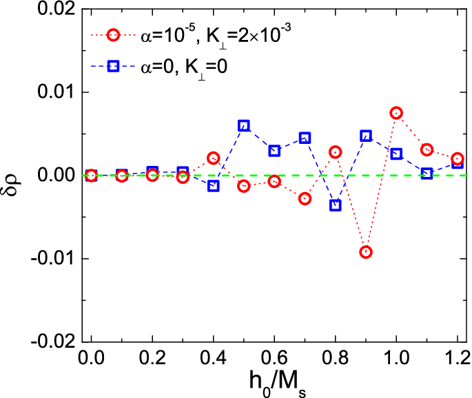
The reflectionless property (total transmission) of the spin wave through DW can also be verified through quantitative analysis of spin-wave amplitude on the two opposite sides of the DW. If the spin wave is monochromatic (a sinusoidal wave) and passes through the DW without reflection, the difference of the spin-wave amplitudes on the two sides of the DW is around zero. We evaluate the spin-wave amplitude difference at $z=-160$ and $z=45$ at the same time, denoted as $\delta\rho$. Figure 3 is the numerical results of $\delta\rho$ as a function of microwave field $h_{0}$. Indeed, $\delta\rho$ is almost zero (green dashed line) both with (circles) and without (squares) damping and transverse magnetic anisotropy. Of course, for nonmonochromatic (sum of many sinusoidal waves) spin waves, the amplitudes on the two sides of the DW may be different at any particular time due to the complicated interference of waves with different frequencies. This is indeed the case for large $h_{0}$, as shown by the oscillatory $\delta\rho$ around zero. The total transmission of spin waves through a DW is an important property because it results in a larger spin-wave spin current, and generates a larger magnonic STT.

Figure 4(a) shows the $h_{0}$ dependence of the spin-wave amplitude $\rho$. It is almost linear at low fields both with (circles) and without (squares) damping and transverse magnetic anisotropy. The behavior is complicated at high fields, and a large error bar of $\rho$ is observed, accompanying less regular and polychromatic spin-wave generation. This also results in a large fluctuation of $\rho$. The $h_{0}$ dependence of the DW velocity $V_{\text{DW}}$ is shown in Fig. 4(b). It is nonmonotonic for the realistic situation with YIG parameters (red circles) and almost quadratic for the case without damping and transverse magnetic anisotropy (blue squares). Although the field dependence of DW velocity is nonmonotonic, the relationship between the DW velocity and the spin-wave amplitude is much simpler. As shown in the inset of Fig. 4(b), the DW velocity $V_{\text{DW}}$ is almost quadratic in $\rho$ both with (circles) and without (squares) damping and transverse magnetic anisotropy. We also plot $\frac{\rho^{2}}{2}V_{g}$ (solid lines) without any fitting parameters, where $V_{g}=1.48$ at $\Omega=0.75$ for the YIG case and $V_{g}=1.61$ at $\Omega=0.85$ in the absence of damping and transverse anisotropy, and $\rho$ is calculated numerically. Although there is no reason why the early velocity formula derived under the approximation of zero damping for uniaxial wire and small spin-wave amplitude should be applicable to the realistic case when both damping and transverse magnetic anisotropy are presented, the theoretical formula is, in fact, not too far from the numerical data for both cases. Of course, it should not be surprising for the deviation at large $\rho$ since quadratic $\rho$ dependence of $V_{\text{DW}}$ is derived based on the conservation of the $z$ component of angular momentum that does not hold for the generic cases. Also the main purpose of the current study is to demonstrate the principles rather than the exact mathematical expression of DW velocity which can be the subject of future studies.

Most studies [12, 13, 14, 24, 26, 27] of magnonic effects in nanomagnetism so far are about the conversion of magnon spins with electron spins. Very often, it goes through the Seebeck effect that involves both thermal and electronic transport. Thus, like usual electronic STT, devices based on these effects must also contain metallic parts so that Joule heating shall be present. In contrast, the magnonic STT presented here does not require electron transport. Devices based on this all-magnonic STT could be made of magnetic insulators like YIG so that the Joule heating is, in principle, avoided. It is also known that the stray field is important in DW dynamics. Our results here are consistent with the OOMMF [28] simulations including this field. Remarkably, these results are consistent with a phenomenological theory on thermomagnonic STT proposed by Kovalev and Tserkovnyak [29].

In conclusion, we proposed an all-magnonic spin-transfer torque mechanism for magnetic domain wall manipulation in nanowires. This spin-transfer torque can effectively drive a DW to propagate along the wires. The propagation speed is sensitive to both microwave frequency and its amplitude. There is an optimal frequency, order of the usual ferromagnetic resonance frequency, at which DW propagating speed is the fastest. All-magnonic STT should have advantages over its electronic counterpart on energy consumption as well as on the spin-transfer efficiency. It also opens the door for using magnetic insulators in spintronic devices.

This work is supported by Hong Kong RGC Grants (No. 604109, No. RPC11SC05, and No. HKUST17/CRF/08).

References

- [1] D.A. Allwood, G. Xiong, C.C. Faulkner, D. Atkinson, D. Petit, and R.P. Cowburn, Science 309, 1688 (2005).
- [2] S.S.P. Parkin, M. Hayashi, and L. Thomas, Science 320, 190 (2008).
- [3] P. Yan and X.R. Wang, Phys. Rev. B 80, 214426 (2009).
- [4] X.R. Wang, P. Yan, J. Lu, and C. He, Ann. Phys. (N. Y.) 324, 1815 (2009); X.R. Wang, P. Yan, and J. Lu, Europhys. Lett. 86, 67001 (2009).
- [5] A. Yamaguchi, T. Ono, S. Nasu, K. Miyake, K. Mibu, and T. Shinjo, Phys. Rev. Lett. 92, 077205 (2004).
- [6] M. Hayashi, L. Thomas, Y.B. Bazaliy, C. Rettner, R. Moriya, X. Jiang, and S.S.P. Parkin, Phys. Rev. Lett. 96, 197207 (2006).
- [7] D.S. Han, S.K. Kim, J.Y. Lee, S.J. Hermsdoerfer, H. Schultheiss, B. Leven, and B. Hillebrands, Appl. Phys. Lett. 94, 112502 (2009).
- [8] M. Jamali, H. Yang, and K.J. Lee, Appl. Phys. Lett. 96, 242501 (2010).
- [9] J. Slonczewski, J. Magn. Magn. Mater. 159, L1 (1996).
- [10] L. Berger, Phys. Rev. B 54, 9353 (1996).
- [11] J. Stöhr and H.C. Siegmann, Magnetism: From Fundamentals to Nanoscale Dynamics (Springer-Verlag, Berlin, 2006).
- [12] M. Hatami, G.E.W. Bauer, Q. Zhang, and P.J. Kelly, Phys. Rev. Lett. 99, 066603 (2007).
- [13] J.C. Slonczewski, Phys. Rev. B 82, 054403 (2010).
- [14] H. Yu, S. Granville, D.P. Yu, and J.P. Ansermet, Phys. Rev. Lett. 104, 146601 (2010).
- [15] S. Yuan, H.D. Raedt, and S. Miyashita, J. Phys. Soc. Jpn. 75, 084703 (2006).
- [16] R. Hertel, W. Wulfhekel, and J. Kirschner, Phys. Rev. Lett. 93, 257202 (2004).
- [17] C. Bayer, H. Schultheiss, B. Hillebrands, and R.L. Stamps, IEEE Trans. Magn. 41, 3094 (2005).
- [18] S. Macke and D. Goll, J. Phys. Conf. Ser. 200, 042015 (2010).
- [19] N.L. Schryer and L.R. Walker, J. Appl. Phys. 45, 5406 (1974).
- [20] A.A. Thiele, Phys. Rev. B 7, 391 (1973).
- [21] R.K. Dodd, Solitons and Nonlinear Wave equations (Academic Press, London, 1982).
- [22] I. Dzyaloshinsky, J. Phys. Chem. Solids 4, 241 (1958); T. Moriya, Phys. Rev. 120, 91 (1960).
- [23] O.A. Tretiakov and A. Abanov, Phys. Rev. Lett. 105, 157201 (2010).
- [24] Y. Kajiwara, K. Harii, S. Takahashi, J. Ohe, K. Uchida, M. Mizuguchi, H. Umezawa, H. Kawai, K. Ando, K. Takanashi, S. Maekawa, and E. Saitoh, Nature (London) 464, 262 (2010).
- [25] M. Krawczyk and H. Puszkarski, Cryst. Res. Technol. 41, 547 (2006).
- [26] G.E.W. Bauer and Y. Tserkovnyak, Physics 4, 40 (2011).
- [27] K. Uchida, J. Xiao, H. Adachi, J. Ohe, S. Takahashi, J. Ieda, T. Ota, Y. Kajiwara, H. Umezawa, H. Kawai, G.E.W. Bauer, S. Maekawa, and E. Saitoh, Nature Mater. 9, 894 (2010).
- [28] M.J. Donahue and D.G. Porter, National Institute of Standards and Technology Interagency Report No. NISTIR 6376, 1999.
- [29] A.A. Kovalev and Y. Tserkovnyak, arXiv:1106.3135.