IFUP-TH/2011-13
Non-Abelian monopole-vortex complex
Mattia Cipriani ,
Daniele Dorigoni ,
Sven Bjarke Gudnason ,
Kenichi Konishi and
Alberto Michelini
(1) Dipartimento di Fisica “E. Fermi” – Università di Pisa,
Largo Pontecorvo, 3, Ed. C, 56127 Pisa, Italy
(2) Scuola Normale Superiore - Pisa,
Piazza dei Cavalieri 7, Pisa, Italy
(3) Istituto Nazionale di Fisica Nucleare – Sezione di Pisa,
Largo Pontecorvo, 3, Ed. C, 56127 Pisa, Italy
(4) Racah Institute of Physics, The Hebrew University,
Jerusalem 91904, Israel
Abstract
In the context of softly broken supersymmetric quantum chromodynamics (SQCD), with a hierarchical gauge symmetry breaking , , we construct monopole-vortex complex soliton-like solutions and examine their properties. They represent the minimum of the static energy under the constraint that the monopole and antimonopole positions sitting at the extremes of the vortex are kept fixed. They interpolate the ’t Hooft-Polyakov-like regular monopole solution near the monopole centers and a vortex solution far from them and in between. The main result, obtained in the theory with equal-mass flavors, is concerned with the existence of exact orientational zero modes, arising from the exact color-flavor diagonal global symmetry. The “unbroken” subgroup with which the naïve notion of non-Abelian monopoles and the related difficulties were associated, is explicitly broken at low energies. The monopole transforms nevertheless according to the fundamental representation of a new exact, unbroken symmetry group, as does the vortex attached to it. We argue that this explains the origin of the dual non-Abelian gauge symmetry.
cipriani(at)df.unipi.it
d.dorigoni(at)sns.it
gudnason(at)phys.huji.ac.il
konishi(at)df.unipi.it
a.michelini(at)sns.it
1 Introduction
The last several years have witnessed a remarkable progress in our understanding of vortex configurations in spontaneously broken gauge theories, which carry continuous, non-Abelian internal zero modes: the non-Abelian vortices [1, 2]. Their rich group-theoretical and dynamical properties have been subject of intense study [3]-[17].
The physics of non-Abelian vortices is deeply related to the understanding of the concept of the non-Abelian monopole and that of the quark confinement, see e.g. Ref.[3]. Indeed, a detailed, fully quantum-mechanical analysis of gauge theories with supersymmetry has given important hints about the low-energy, effective dual gauge symmetry. In particular, fully quantum-mechanical light non-Abelian monopoles appear as the infrared degrees of freedom in the so-called vacua of supersymmetric QCD with quark multiplets, playing the role of the order parameter for confinement (of non-Abelian variety) and for dynamical symmetry breaking [18].
The discovery of the non-Abelian vortex was partly motivated [2] by the desire to understand the physics of the quantum -vacua, , from a more familiar semi-classical viewpoint. In fact, semi-classically the connection between the vortex solutions and regular ’t Hooft-Polyakov monopoles arises from the consideration of a hierarchical gauge symmetry breaking, e.g.
| (1.1) |
The monopole is supported by ; the low-energy vortex solutions correspond to non-trivial elements of . The exact sequence of homotopy groups relates the two solitons of different co-dimension [4], and the global symmetry consideration tells us that the non-Abelian vortex implies non-Abelian monopoles sitting at its extremes. For , one is inevitably led to consider metastable monopole-vortex complex solitons.
The aim of this paper is to pursue further the study of such a monopole-vortex complex, including the numerical analysis of the field configurations involving both the magnetic monopole region and the asymptotic vortex-like region, with all fields approaching smoothly their vacuum expectation value (VEV) away from the complex. In this sense this paper is a continuation of the work by Auzzi et. al. [5]. We clarify also some aspects of the non-Abelian orientational moduli, extensively studied in the last several years in the context of the vortex solutions, and show how the properties of the non-Abelian orientational moduli can be extended to the whole monopole-vortex complex.
The organization of the paper will be the following. In Sec. 2 after a brief introduction of the model we will focus our attention to the main characters of our paper: the vortex and the monopole, a particular care will be given to the study of the symmetries present at different energy scales. In Sec. 3 these two objects will be glued together and we will study the monopole-vortex complex as a whole. We will present both numerical and analytical results concerning the profile functions for the various fields and for the magnetic field, furthermore through a careful identification of the symmetries possessed by the complex we will be able to analyze the low energy dynamics of the orientational zero-modes living on the complex. The conclusions and results obtained in this work are presented in Sec. 4 while we give a more detailed analysis of the full set of equations of motion and the consistency of our Ansatz in the two appendices.
2 The model
To be concrete, we shall work with the softly broken supersymmetric models, due to the many advantages they offer. The fields are those of the gauge multiplet (the gauge field, the gauge fermion, the adjoint scalar and fermion) together with hypermultiplets. To be precise, we take an () gauge theory with flavors of hypermultiplets (quarks), and the mass parameters are tuned such that at two hierarchically different scales the gauge symmetry is broken as in Eq. (1.1). The Lagrangian of the underlying theory has the structure
| (2.2) | ||||
| (2.3) |
where are the bare masses of the quark fields and the complex coupling constant reads
| (2.4) |
The mass of the adjoint chiral multiplet breaks supersymmetry to .
After elimination of the auxiliary fields the bosonic Lagrangian takes the form
| (2.5) | ||||
| (2.6) |
where and the sum over as well as is implicit. In the construction of the monopole-vortex complex soliton solutions it turns out to be sufficient to consider the VEVs and fluctuations around them which satisfy
| (2.7) |
therefore can be set identically to zero in what follows.
The vacuum expectation values (VEVs) of the scalar fields are determined from the minima of the potential following from Eq. (2.6), e.g. see Ref. [18]. They are found to be
| (2.8) | ||||
| (2.9) | ||||
| (2.10) | ||||
| (2.11) |
where the integer
| (2.12) |
labels the possible (classical) vacua. The vacua of a given are further classified according to which set of (out of ) masses are used to construct the solution, leading to the total of
| (2.13) |
As explained in Ref. [18], by choosing a generic set of bare masses and by deforming with the mass term the continuous vacuum degeneracy is lifted altogether, leaving this discrete set of vacua. At small and () the interactions become strong in the infrared, in all these vacua. These are indeed the vacua we are interested in.11 1 This is one of the motivations for considering the system with generic masses and with first, and then eventually taking the equal-mass or massless limit. On the contrary, if we considered directly the massless theory, or equal mass cases, we would find flat directions (continuum vacuum degeneracy); at a generic point along such Higgs branches, the coupling constant remain small at all scales.
By tuning the bare squark masses to an equal, common value , we see that an exact color-flavor diagonal symmetry survives in a vacuum with a given . For definiteness, below we shall work with the classical vacuum where
| (2.14) |
and
| (2.15) |
are obtained by taking such a limit. Note that in this vacuum the gauge group is completely broken; at the same time, however, the color-flavor diagonal global symmetry
| (2.16) |
() remains unbroken by both VEVs. It is an exact global symmetry of the whole system. The system is in the so-called color-flavor locked phase. A hierarchical symmetry breaking pattern (1.1) is realized if
| (2.17) |
Remarks
- (i)
-
The terms containing the adjoint scalar mass play two crucial roles in our model. On the one hand, they induce the small squark condensates, (2.14), bringing the system into a completely Higgsed phase. The existence of the vortex solutions in the low-energy approximation and their properties, all rely on this parameter. Note that due to supersymmetry, the high-energy approximate monopole solution () and low-energy approximate vortex solutions () are both BPS-saturated.
On the other hand, non-vanishing introduces terms in which make both the low-energy vortex and high-energy monopole “solutions” unstable (non-BPS). It is these terms which allow the two solitons of different codimensions to get smoothly combined into a monopole-vortex complex.
- (ii)
-
Of course such a complex “soliton” is not a true solution of the field’s equations of motion; it is only so under the condition that the monopole center positions are kept fixed. Under the assumption of a hierarchical gauge symmetry breaking (2.17), this is not a problem: it is a perfectly sensible (Born-Oppenheimer) procedure, as the motion of the massive monopole can be neglected in the first instance, in the study of low-energy fluctuations of orientational zero modes of the whole complex.
- (iii)
-
Actually the case for working with non-BPS objects as these complex solitons can be made stronger. Just as in the case of the real-world quark-antiquark-chromoelectric string composites (the mesons), our monopole-vortex-antimonopole complex will get stabilized after the quantization of the radial or rotational motions are appropriately taken into account. Of course, only the ground state for each flavor quantum number will be truly stable, as the pair production of the monopole-antimonopole from the vacuum, though suppressed, cannot be rigorously set to zero. But the same holds for the real-world meson states! The fact that these are not topologically stable as static configurations, is therefore not a shortcoming at all; rather it is the necessary price to pay to understand the real-world confinement mechanism.
- (iv)
-
Our semi-classical consideration is valid for the parameter region
As the bare quark masses and the adjoint scalar mass are decreased to small values of the order of , the system becomes strongly coupled and the classical vacua we started with turn into the weakly coupled, dual quantum vacua [18]. This means that the vortex (and monopole) orientational zero modes fluctuate strongly and Abelianize. A possible route to reach the quantum vacua (), where light non-Abelian monopoles appear as the infrared degrees of freedom, through a careful tuning of bare masses and through the consequent vortex solutions with orientational moduli living on , was discussed by some of us in Ref. [6].
2.1 Vortex solution far from the monopole center
In the vacuum (2.14) the -th color component of the squark fields has a mass of the order of and can be integrated away, in the study the low-energy dynamics. At mass scales much lower than the theory is an gauge theory with massless flavors, in the color-flavor locked phase. The vortex solutions in these systems have been a subject of an intense study for the last several years [3]-[17]. A lowest-winding vortex solution oriented in the direction in color-flavor space22 2 These vortices are precisely those studied by [7] for the special case of . The -th color component of the (massive) squark fields is vanishing and not shown in Eq. (2.18). has the form
| (2.18) |
with the profile functions satisfying the appropriate boundary conditions
| (2.19) |
We have introduced above the cylindrical coordinates
which are convenient in the description of the vortex configuration; the gauge field above in fact contains only the component, where is the expression in the square bracket appearing in Eq. (2.18).
The dependent terms in Eq. (2.6), coming from the adjoint scalar mass term , imply that the field behaves non-trivially (Eq. (2.18)): the vortex solution is necessarily non-BPS [7]. Its properties have been carefully studied by Auzzi et. al. [7] in the case of the low-energy , , theory. It has been shown that, independent of the sign of or of , the vortex tension is less than the BPS vortex (for ). The behavior of the profile functions is quite similar, for small , to the case of the BPS vortex analyzed earlier, except for the presence of the small non-vanishing profile functions for in and around the vortex core.
For our purpose below, it is necessary to consider these vortex solutions in a gauge where the scalar quark fields do not wind at infinity. The gauge transformation needed is
| (2.20) |
the vortex solution is indeed transformed into the form
| (2.21) | ||||
| (2.22) |
while the field remains invariant as in Eq. (2.24). In this (singular) gauge all the topological features are hidden into the gauge-field singularity along the vortex core (),
| (2.23) |
The magnetic flux is nevertheless regular everywhere and given by
| (2.24) |
with the components vanishing, so that the total flux is given by
| (2.25) |
Note that such a vortex leaves an subgroup of the color-flavor diagonal global symmetry intact, and as a result develops orientational zero modes living in
| (2.26) |
they are sort of Nambu-Goldstone modes, propagating along the vortex string. More concretely, there is a continuous infinity of degenerate vortex solutions related by
| (2.27) |
Note that the color-flavor matrix belongs to the coset Eq. (2.26) as an individual vortex solution (2.22) preserves the subgroup generated by
| (2.28) |
where the ’s are the standard generators.
The existence of the exact orientational zero modes of Eq. (2.27) possessed by the low-energy vortex solutions characterizes these solitons as non-Abelian vortices [1, 2]. They possess a genuine moduli space of solutions, all having the same tension. Their low-energy fluctuations (i.e. fluctuations carrying energies much lower than the characteristic vortex scale, ) can be shown to be effectively described as a two-dimensional sigma model on . Dynamical features of these fluctuations, detailed moduli-space structures, and their group-theoretic properties have been the focus of considerable attention in the last several years [3]-[17].
Remarks
- (i)
-
Note that even though the light squark fields have only the first color components, the gauge field has a non-vanishing element (see Eq. (2.24) or Eq. (2.22)) due to the fact that the gauge group descends from the underlying gauge group. This turns out to be crucial in the consideration of the vortex-monopole complex below. In this respect, the present model (i.e. the model of [2, 5, 7]), where the theory arises as a low-energy approximation of a spontaneously broken theory, differs essentially from the genuine model studied by other groups [1],[8]-[11], where all scalar and gauge field components live in color space. Even though they share many interesting features of the non-Abelian vortex solutions with our model, it is not possible in these latter models to relate the non-Abelian orientational moduli of the low-energy vortex to the notion of the non-Abelian monopole, which “lives” in the larger gauge group space.
- (ii)
-
When the and coupling constants are set to be equal – this would be the case for the theory just below the higher gauge-symmetry breaking mass scale – the vortex solution above reduces exactly to the Abelian ANO vortex [7], embedded in the corner of the color-flavor space. We shall use below such a simplification e.g. for solving the monopole-vortex complex numerically (Subsection 3.2), but the more general discussion on the orientational moduli (Subsection 3.4) of the complex is independent of it.
2.2 The monopole
As the underlying gauge group is simply connected, the vortex solutions reviewed above cannot be stable in the full theory, which contains the massive monopole excitations. A vortex must end at the two endpoints where monopoles related to the symmetry breaking are situated. The properties of such a monopole solution can be studied to first approximation by neglecting the small VEV, , or equivalently, by studying the system sufficiently close to the monopole center, i.e. at the distances
| (2.29) |
from the center. For and for real neither nor contribute, so the field configuration inside a sphere of such radius should be approximately equal to the standard ’t Hooft-Polyakov BPS monopole solution [19], embedded in an appropriate corner of gauge group. By choosing an group generated by
| (2.30) |
(which is broken to by the VEV of ) a monopole solution can be constructed explicitly as [20]:
| (2.31) |
where33 3 The index refers to the group utilized to construct the solution; the gauge field and the adjoint scalar are both matrices in the color group.
| (2.32) |
is the standard ’t Hooft-Polyakov-BPS solution with
| (2.33) |
the latter behaving asymptotically as
| (2.34) |
(for the antimonopole, ). The constant in the field is added so that it reduces asymptotically to the vacuum expectation value of Eq. (2.14), in a fixed (here chosen as ) direction. The “magnetic flux” emanated from the magnetic monopole is given by
| (2.35) |
which of course is a well-known radial Dirac monopole field, embedded in the color directions.
The ‘‘monopole’’ mass (the energy of the configuration around its center) can be approximately calculated as44 4 We take the adjoint scalar field to be real here and hence normalize it canonically as a real scalar field.
| (2.36) |
Rewriting the Hamiltonian as
| (2.37) |
our monopole configuration is seen to satisfy approximately the non-Abelian Bogomol’nyi equations
| (2.38) |
so that the monopole mass is given approximately by
| (2.39) |
where is in the range (2.29). The monopole mass is, naturally, gauge independent. On the contrary, the “magnetic flux” (2.35) is a gauge dependent quantity. To match the “vortex part” of the solution discussed in the previous subsection, it is necessary to choose a particular gauge in which the adjoint scalar field does not wind at infinity (the so-called singular gauge) in order to describe the complex. By introducing the spherical coordinates
the required gauge transformation is given by
| (2.40) |
where the ’s are the generators of Eq. (2.30). The adjoint scalar field is simply transformed to the fixed direction in the color space (chosen here in the direction):
| (2.41) |
whereas the gauge field has a slightly more complicated form. In view of our task below, of connecting the monopole solution to the low-energy vortex, it is convenient to express the gauge field in the new gauge in the components in the cylindrical coordinate system:
| (2.42) | |||||
where the conversion between spherical and cylindrical coordinates involve the relation
| (2.43) |
while the azimuthal angle is common in the two coordinate systems. The gauge field displays the well-known Dirac string singularity along the negative direction in this gauge:
| (2.44) |
The asymptotic () behavior of the magnetic field can be found by dropping terms multiplied by the factor appearing in Eq. (2.42): only survives and
| (2.45) |
which of course is a well-known radial Dirac monopole field, embedded in the color direction. This radial magnetic field can be seen more easily by directly transforming the asymptotic magnetic field in Eq. (2.35) by , which yields
| (2.46) |
The total magnetic flux through the surface of a sphere of radius around the center, is then given by
| (2.47) |
independently of .
3 Monopole-vortex complex
The equality in the magnitude between the vortex flux (2.25) through a plane perpendicular to the vortex axis, and the magnetic monopole flux (2.47) through the surface of a tiny sphere around the monopole, is an example of the “flux matching” [5, 12], showing that the vortex and monopole together form a smooth soliton complex. Below we elaborate this monopole-vortex complex in more detail.
3.1 Generalities
The first crucial observation is that such a smooth complex requires a compatible orientation between that of the vortex (in the color-flavor mixed space) and that of the monopoles (in the color space). For concreteness and for example the corner of is selected for the winding for the vortex solution Eq. (2.18), and the associated monopole solution is accordingly embedded in the subgroup of the color group, in the plane. Naturally, both the monopole and vortex can be rotated into any other directions by color-flavor transformations; in order to maintain the energy they must be rotated simultaneously (see below).
The relative sign of the flux in Eqs. (2.25) and (2.47) indicates that the monopole studied in the preceding subsection is actually positioned at the rightmost endpoint of the vortex (as in Fig. 4). The outgoing magnetic flux (in the direction of ) of the monopole is carried away in the vortex bundle on its left.
Another crucial observation is about the behavior of the gauge field. The monopole field in the “singular” gauge, Eq. (2.42), exhibits the well-known Dirac string singularity along the negative direction, Eq. (2.44). This behavior matches precisely that of the gauge field along the vortex core, Eq. (2.23), confirming further the relative positioning of the vortex with respect to the monopole. The Dirac string singularity Eqs. (2.23),(2.44) is entirely harmless as it appears multiplied by the squark field in the squark kinetic term ; the latter drops to zero along the vortex core. The color magnetic field is smooth everywhere, as noted already.
Note that the choice of the particular gauge (the so-called singular gauge) needed for matching the Dirac singularity of the gauge field, is precisely the one which guarantees the smooth field configuration everywhere. In particular, in this gauge no fields “wind” around either the vortex axis or the monopoles. The scalar fields approach their vacuum expectation value everywhere outside the complex, as in Eqs. (2.21) and (2.41). See Fig. 3.
In order to describe the field configurations interpolating the vortex and monopole, , we make an Ansatz of the form
| (3.48) |
The profile functions , with appropriate boundary conditions, can be determined numerically as we will do in the following section.
3.2 Numerical solution
In order to study these configurations numerically, we note that if the and coupling constants are set to be equal our monopole-vortex complex is exactly the monopole-vortex complex generated by the symmetry breaking
| (3.49) |
embedded in a larger color-flavor space. It is therefore sufficient for our purpose here to consider the minimal case, Eq. (3.49). The generators of the group are , where are the Pauli matrices and the scalar field has the form:
where is the fluctuation around the VEV. The Lagrangian is then:
| (3.50) |
where we have set
and our convention for the covariant derivatives and field strength is
| (3.51) | ||||
| (3.52) | ||||
| (3.53) |
After the symmetry breaking at , the second color component of the squark field becomes massive, so we can set
The equations of motion for the system are:
| (3.54) | ||||
| (3.55) | ||||
| (3.56) |
where we have defined . In order to solve these equations numerically, we introduce an Ansatz adequate for the theory, which is somewhat simpler than Eq. (3.48):
| (3.57) |
Substituting this Ansatz into the equations of motion, written extensively in Eqs. (B.93)-(B.95), one obtains the coupled differential equations Eqs. (B.97a)-(B.97g). A priori this system of equations seems to be an overdetermined system with respect to the function . However as we have shown in the previous sections, the chosen Ansatz is well suited for both the monopole and the vortex, and hence we have assumed the existence of a solution to all the equations, solving only the system (B.97d,B.97e,B.97f,B.97g). After the solution was obtained, we plugged it into the constraint equations (B.98a-B.98b) as well as the remaining second order equation (B.97b) and indeed verified that the solution satisfies all equations.
In solving the system of these differential equations the relaxation method is very useful. We introduce a fictitious time dependence into each of the profile functions and then write all the equations as:
| (3.58) |
where denotes the equation of motion for the profile function , which is obeyed when . It is important that the equation is of second order in spatial derivatives and that the sign of the Laplace operator is positive: with summing over spatial dimensions. In this way the equation with the fictitious time-dependence resembles (a modified form of) the well-known heat equation, and when a stationary solution has been found, i.e. the equation of motion for has been obtained.
First we need to impose some reasonable initial conditions (i.e. a guess of the right solution) for the profile functions at and let the system evolve till a static solution is found. This was done by patching together three different solutions to the equations of motion. The first solution is the non-BPS solution of the vortex (of infinite length), which is easily obtained numerically, see Fig. 2 and also [7]. The second solution needed is for the monopole and here it turned out to be most efficient to simply use the analytical solution of the BPS ’t Hooft-Polyakov monopole. The third solution is simply the Higgs vacuum. Now patching the solutions together by using a piecewise function in the coordinates, we obtained an initial “solution”, see Fig. 1.

The final ingredient in the solving the vortex-monopole complex is probably the most crucial, namely the boundary conditions. Physical arguments tell us that the complex is not really semi-classically stable as it stands. Hence, one could worry that the relaxation method would shrink the system to merely the Higgs vacuum. In order to circumvent that, we implemented the boundary conditions for the system very similarly to what we did for Abelian soliton junctions in Ref. [21], viz. fixing the monopole positions and hence the string length. In this way, the complex is a minimum of the energy – given the condition we impose. In Fig. 1 we have also shown the boundary conditions (BCs). The three sides far from the complex all have Dirichlet BCs, i.e. the Higgs vacuum. At the vortex string in the middle of the -axis also Dirichlet BCs are imposed, namely the non-BPS vortex solution described above is used as the boundary condition – this is what fixes the string length. For the remaining pieces on the -axis, we have imposed Neumann BCs due to cylindrical symmetry of the problem.
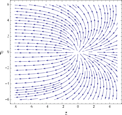
The numerical calculation55 5 The numerical analysis has been done with the Mathematica package. gave the results shown in Fig. 3 for the profile functions , , , and . Note that both scalar fields (the adjoint and fundamental) approach their VEVs smoothly far from the monopole-vortex complex in all directions. The monopole-vortex complex is immersed in the Higgs vacuum. Far from the monopole centers, the fields reduce to those of the (non-BPS) vortex, Fig. 2, whereas they reduce to the ’t Hooft-Polyakov monopole solution in the small spherical region near the monopole center.
These profile functions give rise to the magnetic field shown in Figs. 4 and 5; as expected the magnetic flux coming out of the monopole (isotropically near the monopole center and in the direction of ) is carried away in a vortex bundle located on its left, and gets reabsorbed by the antimonopole sitting at the far left extreme of the vortex.




3.3 Macroscopic picture and duality
Recently the monopole-vortex complex in the simplest gauge symmetry breaking (3.49)
| (3.59) |
has been discussed [22, 23] in the London limit, in this limit the monopole is a point and the vortex a line, without width. In this approximation it is possible to perform the electromagnetic duality transformation explicitly, and the resulting dual theory can be solved for the electric and magnetic fields explicitly, in the presence of the monopole-vortex complex. In the presence of a static heavy monopole of unit charge sitting at , and with a semi-infinite vortex extending on its left, the magnetic (and electric if ) fields are given by [23]
| (3.60) |
where
| (3.61) |
and is the Green function, having the Yukawa form
| (3.62) |
Such a construction, in the case of a more general symmetry breaking
and in the presence of a color-flavor diagonal symmetry, is not known; but as noted above, in the approximation the results, Eqs. (3.60)-(3.62), represent the color-magnetic or electric flux in the direction (Eq. (2.30)).
3.4 Orientational zero modes
Let us now return to the symmetry breaking of our interest here
| (3.63) |
and consider the monopole-vortex complex (3.48). The color-flavor diagonal symmetry (2.16) is an exact symmetry of our system in the Higgs phase: it is not an approximate symmetry of the low-energy gauge system. On the other hand, the monopole-vortex complex (3.48) is not invariant under the full symmetry: it transforms as
| (3.64) |
where . Of course, not all elements transform the configuration non-trivially. The complex (3.48) is obviously invariant under the subgroup generated by
| (3.65) |
The subgroup of , generated by
| (3.66) |
acts in a subtler way on the monopole-vortex complex. The pure vortex configuration (2.24) of the low-energy theory is clearly invariant under such a transformation, but the monopole-vortex complex is not obviously invariant.
The problem is that the complex (3.48) lives in a larger, gauge space, i.e. it has necessarily non-vanishing color components in the -th row and/or -th column. However, decomposing Eq. (3.66) as
in terms of two, matrices, one sees that is invariant under transformations whereas they transform under simply as
| (3.70) |
This can be easily seen to be equivalent to the shift of the azimuthal angle
| (3.71) |
in other words, it is equivalent to (i.e. can be undone by) a spatial rotation of angle around the monopole-vortex axis, .
3.5 Demise and resurrection of the symmetry
In the small region around the monopole, (2.29), the tiny VEV may be effectively set to zero; as the squark fields are then trivial () the transformations (3.64) look locally as global color transformations of the monopole solution.
This shows that the isomorphism between the vortex moduli [2] and the monopole moduli66 6 Here we neglect the zero modes related to the electric charge of the monopole; in the Higgs phase they survive only in the vicinity of the monopole center. See also Ref. [23]. – both found to be – is certainly not a coincidence. Nevertheless, attempts to understand the moduli space of the monopoles (representing ) as something arising from its various possible embeddings in the larger color space , face inevitably the known difficulties:
- (i)
Topological obstruction [24];
- (ii)
Non-normalizable gauge zero modes [25];
- (iii)
Non-local nature of Goddard-Nuyts-Olive (GNO) duality [26] .
The first two issues have been discussed many times in the literature, and need not be reviewed here (see however below for observations concerning these points). It is perhaps worthwhile however to recall the third point, which is apparently the simplest of the three and at the same time, the deepest. The GNO quantization condition [26]
| (3.74) |
where are non-vanishing root vectors of , and where the asymptotic gauge field is written as (in an appropriate gauge)
| (3.75) |
in terms of the Cartan subalgebra generators of , tells us that the set of degenerate monopoles are labeled by the dual weight vector . The duality implied by such a formula is clearly a natural generalization of the electromagnetic duality. The transformations of the monopole under the dual, magnetic group correspond to some non-local field transformations in the original description77 7 The fact that in most papers in which these issues are discussed the gauge group is taken to be appears to have helped to obscure this point, as the dual of is again . It is however sufficient to generalize the discussion, for instance, to the case of a gauge symmetry breaking (3.76) in this case the monopole transforms according to the dual of : under . The monopoles are predicted to transform according to one of the dimensional spinor representations [13].. Simply, it is not the right question to ask how the monopole solutions associated with the gauge symmetry breaking transform under the “unbroken” global color subgroup .
Let us return to the symmetry breaking (3.63)
| (3.77) |
The “magnetic monopole” solution arising from the breaking at the scale cannot be rotated without spending energy under the : the latter is broken by the smaller squark VEV, , Eq. (2.14). It costs energy to vary the embedding of the subgroup within the (Eq. (2.30)), as the squark fields have a preferred color-flavor locked direction (Eq. (2.22)). Forcing so (rotating the embedding) would distort the complex and yield a higher-energy configuration (an excited state). In other words, the subtle issues of the non-normalizable zero modes and the topological obstruction for defining the global color (i) and (ii), have been converted into an explicit breaking of the symmetry.
However, the system has an exact color-flavor diagonal symmetry. Individual monopole-vortex complex configurations break it. They live in the continuous moduli of the solution space
The simultaneous color-flavor transformations acting on the original fields keep the energy unchanged; they induce movements on . The complex transforms as in the fundamental multiplet of an .
This then represents a new, exact non-Abelian symmetry for the monopole: the latter transforms according to the fundamental representation of an group.
The fluctuations of the associated zero modes propagate only along the vortex; this makes sense because, according to the standard lore, the dual gauge group is in a confinement phase, the original local gauge group being in the Higgs phase. The monopoles are confined by the color-magnetic vortex, which in the dual picture represents the color-electric confining string.
4 Conclusion
In this paper we elaborated further on some earlier analyses [5, 4] of the monopole-vortex complex “soliton”, arising in systems with hierarchically broken gauge symmetries. In a vacuum with an exact unbroken color-flavor symmetry (color-flavor locked phase), such a complex acquires orientational zero modes, analogous to those extensively studied recently in the context of non-Abelian vortices [3]-[17]. The field configurations are studied both qualitatively and numerically, verifying that they constitute a smooth “constrained” minimum of the energy, with the monopole and antimonopole positions kept fixed. The whole complex possesses the orientational degeneracy (arising from the exact color-flavor symmetry): it implies a new, exact continuous symmetry for the monopole, confined by the vortex. This, we argue, is the semi-classical origin of the dual gauge symmetry. Their fluctuations propagate in the monopole-vortex-antimonopole worldsheet strip, the monopole and antimonopole acting as the source or sink for the massless (Nambu-Goldstone like) excitations, propagating along the vortex in between. Extending the direct derivation of the vortex worldsheet sigma models on [2, 9, 10] (or in Hermitian symmetric spaces, , , etc., depending on the model considered [13]) to the case of monopole-vortex complex is a somewhat non-trivial task, presently under investigation. Our microscopic study here should serve as the basic starting point for such an analysis.
Acknowledgments
SBG gratefully acknowledges a Golda Meir post-doctoral fellowship. DD thanks Collège de France and Fondation Hugot for the hospitality and support during the revision of this paper. The authors thank J. Evslin and T. Fujimori for discussions.
Appendix A BPS monopole and vortex solutions
Here we will briefly check that the BPS equations for the monopole and the vortex are compatible with our second-order equations of motion.
A.1 Monopole
Let us start with the monopole; the BPS equation reads:
| (A.78) |
while the covariant derivative of the latter can be written as
| (A.79) |
where we have used the BPS equation in the last equality. This equation agrees with Eq. (3.54) in the BPS limit, with real (taking into account a factor of for the canonical normalization of the kinetic term) and setting .
A.2 Vortex
The vortex BPS equations are for
| (A.81) | ||||
| (A.82) | ||||
| (A.83) |
where the upper (lower) sign gives a BPS vortex (anti-vortex) and is the adjoint index (in the case only the first of the gauge equations appears). We consider here a symmetry breaking pattern like and the BPS equations come about at low-energy in this system in the limit of while is kept constant. We will check this explicitly below.
General case:
The Lagrangian of the system is
| (A.84) |
which leads to the equations of motion
| (A.85) | ||||
| (A.86) | ||||
| (A.87) |
where is the adjoint index and . Let us now truncate the theory to the low-energy sector, i.e. we will integrate out the massive components of the squarks and also the adjoint and gauge fields corresponding to broken generators, as they will have a mass of the order of . The vortex solution requires , (which is the adjoint field written in terms of the group with corresponding index ) to be fixed at the VEV . As already mentioned the BPS limit corresponds to taking , with the product kept finite. We have: . Hence, in this limit the second equation is trivially satisfied.
For the first equation we have:
| (A.88) |
We can combine the Eqs. (A.81) and (A.82) by setting the two coupling constants to be equal; (and choosing the upper sign) which yields
| (A.89) |
Acting with the covariant derivative yields (note that it acts in the adjoint way on both terms)
| (A.90) |
where we have used the BPS equation (A.83) in the last step. Multiplying by and taking the trace gives us Eq. (A.88).
Appendix B Numerical analysis in theory
Writing out the equations of motion Eqs. (3.54)-(3.56) explicitly in terms of the fundamental fields gives:
Gauge fields
| (B.93) | ||||
Scalar fields
| (B.94) |
Squark fields
Constraint equations
| (B.98a) | |||
| (B.98b) | |||
References
- [1] A. Hanany and D. Tong, JHEP 0307 (2003) 037 [arXiv:hep-th/0306150].
- [2] R. Auzzi, S. Bolognesi, J. Evslin, K. Konishi and A. Yung, Nucl. Phys. B 673 (2003) 187-216 [arXiv:hep-th/0307287].
- [3] K. Konishi, in Lecture Notes in Physics, 737 (2008) 471, Springer [arXiv:hep-th/0702102].
- [4] M. Eto, L. Ferretti, K. Konishi, G. Marmorini, M. Nitta, K. Ohashi, W. Vinci and N. Yokoi, Nucl. Phys. B 780 (2007) 161 [arXiv:hep-th/0611313].
- [5] R. Auzzi, S. Bolognesi, J. Evslin and K. Konishi, Nucl. Phys. B 686 (2004) 119 [arXiv:hep-th/0312233].
- [6] D. Dorigoni, K. Konishi and K. Ohashi, Phys.Rev. D 79 (2009) 045011 [arXiv:hep-th/0801.3284].
- [7] R. Auzzi, M. Eto and W. Vinci, JHEP 0711 (2007) 090 [arXiv:hep-th/0709.1910].
- [8] A. Hanany and D. Tong, JHEP 0404 (2004) 066 [arXiv:hep-th/0403158].
- [9] M. Shifman and A. Yung, Phys. Rev. D 70 (2004) 045004 [arXiv:hep-th/0403149].
- [10] A. Gorsky, M. Shifman and A. Yung, Phys. Rev. D 71 (2005) 045010 [arXiv:hep-th/0412082].
- [11] M. Eto, Y. Isozumi, M. Nitta, K. Ohashi and N. Sakai, Phys. Rev. Lett. 96 (2006) 161601 [arXiv:hep-th/0511088].
- [12] M.A.C. Kneipp, Phys. Rev. D 69 (2004) 045007 [arXiv:hep-th/0308086].
- [13] S.B. Gudnason, Y. Jiang and K. Konishi, JHEP 1008 (2010) 012 [arXiv:hep-th/1007.2116].
- [14] Y. Isozumi, M. Nitta and K. Ohashi et al., Phys. Rev. Lett. 93 (2004) 161601 [arXiv:hep-th/0404198].
- [15] D. Tong, Phys. Rev. D 69 (2004) 065003 [arXiv:hep-th/0307302].
- [16] M. Eto, T. Fujimori, S.B. Gudnason, K. Konishi, M. Nitta, K. Ohashi and W. Vinci, Phys. Lett. B 669 (2008) 98 [arXiv:hep-th/0802.1020]; M. Eto, T. Fujimori, S.B. Gudnason, K. Konishi, T. Nagashima, M. Nitta, K. Ohashi and W. Vinci, JHEP 0906 (2009) 004 [arXiv:hep-th/0903.4471].
- [17] M. Eto, S. B. Gudnason, J. Phys. A A44, 095401 (2011). [arXiv:1009.5429 [hep-th]].
- [18] G. Carlino, K. Konishi and H. Murayama, JHEP 0002 (2000) 004 [arXiv:hep-th/0001036]; Nucl. Phys. B 590 (2000) 37 [arXiv:hep-th/0005076].
- [19] G. ’t Hooft, Nucl. Phys. B 79 (1974) 276; A.M. Polyakov, JETP Lett. 20 (1974) 194.
- [20] E. J. Weinberg, Nucl. Phys. B 167 (1980) 500; Nucl. Phys. B 203 (1982) 445.
- [21] S. Bolognesi, S. B. Gudnason, Nucl. Phys. B754, 293-308 (2006). [hep-th/0606065].
- [22] C. Chatterjee and A. Lahiri, JHEP 1002 (2010) 033 [arXiv:hep-th/0912.2168].
- [23] K. Konishi, A. Michelini and K. Ohashi, Phys.Rev. D 82 (2010) 125028 [arXiv:hep-th/1009.2042].
- [24] A. Abouelsaood, Nucl. Phys. B 226 (1983) 309; P. Nelson and A. Manohar, Phys. Rev. Lett. 50 (1983) 943; A. Balachandran, G. Marmo, M. Mukunda, J. Nilsson, E. Sudarshan and F. Zaccaria, Phys. Rev. Lett. 50 (1983) 1553; P. Nelson and S. Coleman, Nucl. Phys. B 237 (1984) 1.
- [25] N. Dorey, C. Fraser, T.J. Hollowood and M.A.C. Kneipp, Phys.Lett. B 383 (1996) 422 [arXiv:hep-th/9512116].
- [26] P. Goddard, J. Nuyts and D. Olive, Nucl. Phys. B 125 (1977) 1.