Tunnelling Methods and Hawking’s radiation: achievements and prospects
Abstract
The aim of this work is to review the tunnelling method as an alternative description of the quantum radiation from black holes and cosmological horizons. The method is first formulated and discussed for the case of stationary black holes, then a foundation is provided in terms of analytic continuation throughout complex space-time. The two principal implementations of the tunnelling approach, which are the null geodesic method and the Hamilton–Jacobi method, are shown to be equivalent in the stationary case. The Hamilton–Jacobi method is then extended to cover spherically symmetric dynamical black holes, cosmological horizons and naked singularities. Prospects and achievements are discussed in the conclusions.
1 Introduction
Since the discovery of quantum black hole thermal radiance by Hawking [1] (extremely good reviews and surveys are in [2], [3], [4], [5] and [6]), it became pretty clear that something remarkable concerning the interface of gravity, quantum theory and thermodynamics was at work. In the usual picture, a radiating black hole loses energy and therefore shrinks, evaporating away to a fate which is still debated. Many new ideas came out from the recognition that quantum field theory implied a thermal spectrum: the most impressive probably being ’t Hooft’s idea of a dimensional reduction in quantum gravity and the associated holographic description (indicating a drastic reduction in the counting of degrees of freedom in finite regions, which scale with area rather than volume) [7, 8]; and the principle of black hole complementarity aimed to reconcile the apparent loss of unitarity implied by the Hawking process with the rest of physics as seen by external observers [9]. But there were also other, more practical, issues regarding these matters, some of which bewildered scientists since the very beginning and that have been only partly resolved. A key issue is that the original derivation of Hawking radiation applied only to stationary black holes, while the picture above uses quasi-stationary arguments. Actually, an evaporating black hole is non-stationary. Nevertheless, a surprising aspect of the semi-classical result is that the radiation caused by the changing metric of the collapsing star approaches a steady outgoing flux at large times, implying a drastic violation of energy conservation. This certainly means that one cannot neglect the back-reaction problem which, however, has not been solved yet in a satisfactory way. A sample of other key issues have to deal with the final state of the evaporation process, the thermal nature and the related information loss paradox, the Bekenstein–Hawking entropy and the associated micro-states counting, the trans-planckian problem, and so on. It was to address some of these questions that some alternative derivations and descriptions of the Hawking’s emission process began to appear over the years [10, 11, 12, 15, 16, 13, 17, 14, 18], one of these being the so called tunnelling method, the leitmotiv of this review.
Before introducing it in full mathematical detail, we shall spend the next few paragraphs
to spell out some general features of this method and how it compares with the general
properties of quantum fields and states in the presence of a black hole11
1
For those
interested, an up to date resource for papers, books and other stuff about black hole
physics and astrophysics is the “Resource Letter BH-2: Black holes” by Marolf and
Gallo [19]..
The tunnelling method has to do with the particle interpretation of the emission process, which would be the most natural way to explain the loss of energy suffered by the radiating black hole, but also poses a problem. It is that while the original derivation of Hawking radiation used the theory of quantum free fields propagating in a fixed gravitational background, for the case at hand a particle interpretation in the near horizon region of a black hole space-time was found to be far from unique and therefore inherently ambiguous. This fact is deeply rooted into the physical nature of the problem, which is that the general covariance of the physical laws allows many inequivalent choices of time, as was explained several times (see, e.g. [20, 21]). It was partly to overcome such difficulties that DeWitt launched in the Seventies the “stress-energy-tensor program” aimed to compute the expectation values of the stress tensor and other observables to better describe quantum effects in a curved space-time [22]. Thus, it was found that it is not in general possible to divide into a real particle contribution and a vacuum polarisation part in an unambiguous way. However, it will always be possible to choose any coordinate system, as long as it is regular across the horizon, and use it to define an observer dependent vacuum relative to which a particle definition is feasible. As we will see, with the tunnelling method we are only concerned with the probability that such an observer dependent notion of particle be emitted from the horizon of the black hole. If this probability is a coordinate scalar it will not depend strongly on what particle concept one employs. In fact, we can call it a click event in a particle detector if we like, without committing ourselves with the particle concept; concept which remains of great heuristic value however, and will find its realisation in the choice of the particle action used to compute the tunnelling probability. Such an observer dependent notion of particles has been advocated also by Gibbons and Hawking in their treatment of de Sitter radiation [23], on the ground that an observer independent definition of particles is not relevant to what a given observer would measure with a particle detector.
The second aspect we would like to mention is the fact that, as it will be seen, the tunnelling
method uses only the classical action of a single massless, spin-less particle and therefore
appears to be state independent. It does what it does by relating the particle emission to
an imaginary contribution to the classical action localised at the horizon, which only
comes from the local geometry. This can be traced back to the work of Damour and
Ruffini [24] with contributions of Padmanabhan et al.
[25, 26, 27, 28], Massar and Parentani
[29] and Kraus and Wilczek, Parikh and Wilczek [30, 31, 32] (see also Kraus’s Ph.D. thesis [33]). To what extent this is so was recently studied in [34] where, for a large
class of quantum states with Hadamard short distance singularity, it was shown that the two-point correlation function, which is directly related to the tunnelling probability, has a universal thermal appearance whose temperature is, needless to say, the Hawking temperature.
Now all these important findings have the drawback that they have been proved, and one can easily understand why, only for stationary black holes. In that case the tunnelling picture has not much more to say than was already known, at least for the simplest solutions, besides helping to understand black hole radiation from a different viewpoint. Where exact calculations can be done, it typically gives a less detailed picture of the radiation process since it is mainly related to a semi-classical emission rate. The cases where the method is more powerful have to do either with more intricate stationary solutions or else with truly dynamical black holes. We can list here some of its achievements and properties:
- 1.
The estimation of the leading correction to the semi-classical emission rate arising from back-reaction to the background geometry, whose introduction by Kraus and Wilczek, Parikh and Wilczek [30, 31, 32] motivated the tunnelling method in a form that will be discussed soon; its extension to Anti–de Sitter (AdS) [35], de Sitter (dS) [40, 36, 37, 38, 39] and higher dimensional black holes; the existence of correlations among successive emission events [41, 42, 43];
- 2.
The original tunnelling method can be generalised to a Hamilton–Jacobi variant, originated with the work of Padmanabhan and collaborators [25, 26, 27, 28] and systematically applied either to stationary or dynamical black holes (see e.g. [44, 46, 48, 47, 12, 45, 49] for a sample of papers). For dynamical black holes this was particularly important, since even approximate quantum calculations are notoriously hard. Moreover, in this variant it manifestly preserves general covariance;
- 3.
Supplemented with a more precise and more general mathematical definition of a local horizon, the Hamilton–Jacobi variant can be applied to any sort of horizon within this class, and in particular to cosmological and weakly isolated horizons [50] (for definitions see below). It can also be applied to past horizons and white holes, in which case a clear notion of temperature emerges in complete analogy to black holes;
- 4.
The tunnelling method strengthens the connection of the semi-classical rate with the surface gravity of the horizon even for dynamical black holes, provided that opportune definitions of such quantities are employed. In this respect its application to extremal black holes should have something to say;
- 5.
The tunnelling picture can promptly give indications on what occurs in other situations. One example is the WKB approach to Unruh’s radiation, reviewed in [51]. It can also be applied to see whether naked singularities are going to emit radiation, or to study the decay of unstable particles that in the absence of gravity would be stable by the action of some conservation law. This is valuable given the great efforts that are normally necessary to analyse quantum effects in the presence of gravity.
It remains to explain how the tunnelling picture works and to what extent it gives a consistent picture, at least from a logical point of view. This will cover the rest of this review whose structure, we anticipate, will essentially follow the material just indicated in listed form above.
In Section 2, the methodological core of the topic is outlined and applied to various stationary solutions. In Subsection 2.1 we present the original method introduced by Parikh and Wilczek to study the black hole radiance — namely the null geodesic method — which is subsequently applied to verify the thermal properties of a static, spherically symmetric Schwarzschild black hole in the scalar sector. In Subsection 2.2 we comment results pertaining to statistical correlations of successive emission events, as displayed by the tunnelling method. In Subsection 2.3 and Subsection 2.4, after pointing out some flaws of this approach, we extend it to the more recently conceived Hamilton–Jacobi tunnelling method: this approach is examined in great detail in order to stress those points that — given the vastness and heterogeneity of opinions in the literature — might lead to confusion. In Subsection 2.5 we present the extension of the Hamilton–Jacobi tunnelling method to the fermionic sector. The description of the tunnelling phenomenon in non-static, but still stationary space-times is undertaken in rest of the section: starting from the Kerr and Kerr–Newman solutions in Subsection 2.6, we then conclude the section showing in Subsection 2.7 more peculiar scenarios — such as non axis-symmetric or lower and higher-dimensional solutions.
In Section 3, we study the mathematical foundation of the two tunnelling methods. The Hamilton–Jacobi method, preferable in view of its manifest covariance, is examined in Subsection 3.1. It is found to be equivalent to the null geodesic method, at least in its generalised form, in Subsection 3.2. The aforementioned variety of opinions also comprehends a number of alternative proposals to the two methods, some of which are summarised in Subsection 3.3.
In Section 4, we approach the dynamical case but restricting ourselves to spherically symmetric non vacuum black holes. Though it may appear strange that stationary black holes, being a particular case of dynamical ones, are discussed first, there is a reason: in the stationary case there is much more control on the mathematics of the tunnelling picture. In particular, it is possible to use both the null geodesic method as well as its Hamilton–Jacobi variant to deduce the exact semi-classical thermal spectrum of the Hawking radiation, a fact which greatly enhances the understanding of the tunnelling picture in a way which is not available to dynamical situations. At the same time it provides the foundation for the dynamical treatment and inspires extensions to more general cases. The Section is further divided into several sub-sections. In Subsection 4.1 we describe various definitions that have been proposed over the years to characterise a black hole horizon and corresponding definitions of the surface gravity. Again few dynamically inequivalent definitions will be reviewed, putting particular emphasis on the one which the tunnelling method privileges. In Subsection 4.2 we review material pertaining to spherically symmetric space-times and the form that surface gravities and horizons take in this highly symmetric case. In Subsection 4.3 we finally come to grasp the tunnelling mechanism. After a careful scrutiny of the escaping paths we derive the basic results; the computation of the imaginary part of the action, its relation with the surface gravity and the ensuing quasi-thermal interpretation.
In Section 5, we discuss how the tunnelling picture generalises to cosmological horizons, naked singularities and particle decays. We shall see that the first two cases are governed by a simple pole singularity while decays correspond to branch cut singularities of the classical action. In Subsection 5.1 we review few facts regarding Friedmann–Robertson–Walker space-times (abbr. FRW) with emphasis on the existence of horizons, their structure and surface gravity. In Subsection 5.2 we apply the tunnelling method to cosmological horizons and find their emission rate. In Subsections 5.3 and 5.4 we analyse its application to particle decays and particle creation by black hole singularities. The former was extensively studied in de Sitter space-time, where exact results can be obtained, but the tunnelling method is not restricted to particular space-time choices. In Subsection 5.5 we review the possibility that naked singularities themselves radiate away their (suitably defined) mass. Indications of this phenomenon are supported by the tunnelling method.
We end with Section 6 where achievements, prospects and conclusions are summarised.
As a final note, since we found the literature on quantum tunnelling to be quite extensive22 2 An INSPIRE search gave us more than 500 records about tunnelling from black holes, to date., the references will not exhaust all the existing literature. We struggled to cover a lot of papers, and especially those that appeared more meaningful to our eyes, being aware that this will inevitably come to reflect some personal taste. A sample of the vast literature is here collected for the reader’s benefit, beyond those already cited. For studies on tunnelling from a general point of view see [196]; tunnelling of fermions and bosons from stationary black holes in asymptotically flat, de Sitter or anti-de Sitter spaces and other exotic objects in several coordinate systems were considered in [197]; tunnelling of bosons and fermions in higher and lower dimensions are covered in [198]; for contributions to dynamical black holes see [199], for cosmology [200]. Our sincere apologies are directed to the many unwittingly omitted.
We shall use the following conventions throughout: the metric signature is ; the constants , , and set equal to unity unless explicitly stated; we use an index notation for tensor components. Greek indices are used to denote space-time components of a tensor; mid-Latin indices as are typically used to denote the component; late-Latin indices as for purely spatial tensors part. If not otherwise stated, an overdot will represent a time derivative, and a prime a spatial derivative in the (case by case) relevant spatial coordinate.
2 Quantum Tunnelling: Stationary Black Holes
According to quantum field theory, the physical vacuum – the state with no real particles – is in general a complex entity populated by virtual particles which constantly are created, interact among themselves and are then annihilated in this vacuum. In the absence of external fields, the vacuum is usually stable in the sense that virtual particles are not able to survive long enough to become real. However, it is now well proved that external fields are able to convert short-living particles into real ones just supplying enough energy to the process.
Considering particle creation by a static gravitational field endowed with a Killing vector , the energy of a particle is , where is the particle’s four-momentum. For massive (massless) particles, the momentum is a future-directed time-like (null) vector. Thus, the energy of a particle is always positive in the region where the Killing vector is also future-directed and time-like. It follows that particle creation in a space-time region with future-directed and time-like is forbidden by energy conservation. Such considerations provide a heuristic argument [52] to conclude that a static gravitational field can create particles only if the space-time contains a black hole. In fact, when a virtual particle pair is created just inside the horizon, the positive energy virtual particle can tunnel outside — no classical escape route existing — where it materialises as a real particle; in alternative, for a pair created just outside the horizon, the negative energy virtual particle, forbidden outside the horizon, can tunnel inwards [53]. In either cases, the negative energy particle is absorbed by the black hole, resulting in a black hole mass decrease, while the positive energy particle escapes to infinity, visible to distant observers (Hawking radiation).
In 1974 Hawking [1] proved that indeed black holes are classically stable objects that, due to quantum fluctuations, become unstable with respect to particle emission. Nowadays, several methods are known for deriving Hawking radiation and calculating its temperature, but none of them has been able to catch the intuitive picture above as the tunnelling method proposed a decade ago by Parikh and Wilczek [32]: it were not for the inclusion of back reaction, their method could be considered a semi-classical version of Hartle–Hawking’s path integral derivation of black hole radiance [54].
2.1 The null geodesic method
The so called null geodesic method — as named by Kerner and Mann [46] — derives black hole radiance from few reasonable assumptions, namely: energy conservation, detailed balance and the use of non-singular coordinates across the horizon.
Energy conservation requires fixing the total energy of the space-time before and after
particle emission. Since black hole mass and volume are linked together, a mass
reduction due to the emission of a particle translates into a size contraction; so one might
worry how to deal with quantum fluctuations of the metric originating from such
contraction. However, this is not a problem as far as we consider transitions between
zero-spin geometries. In this case in fact, no graviton quantisation is involved or, said in
other words, passing from different spherically symmetric configurations does not
produce gravitational waves. As a consequence, the only degree of freedom remained in
the problem is the position of the emitted particle (actually, a thin shell). Thus, to keep
things as simple as possible, we can restrict to consider uncharged, static, spherically
symmetric black holes emitting neutral matter, referring to next sections treatment of the
most general case.
Because of Birkhoff’s theorem [55], we are dealing with Schwarzschild geometry which, written in the Schwarzschild frame, reads
| (2.1) |
where the gravitational radius is . Computing the free fall acceleration of a body initially at rest in the Schwarzschild frame, we get
| (2.2) |
The geometry (2.1) becomes singular at the gravitational radius and the
acceleration (2.2) becomes infinite in the same limit. Nonetheless, near
the space-time is regular (i.e. neither curvature singularities or geodesic
incompleteness): an indication of the fact that the Schwarzschild frame ceases to be
defined at (For systems must be non-rigid in
the sense that the metric components must be functions of time, cf.
[52]).
It is well-known that the gravitational radius represents the Killing event
horizon of Schwarzschild black hole [55]; thus, in order to deal with
tunnelling of a particle across it, we need to cover the region with
regular coordinates. A possible choice, not the only one, is represented by Painlevé–Gullstrand coordinates [56]. In order to construct this new regular-across-the-horizon frame, we consider the geodesic equations of a family of observers, freely falling
() in the geometry (2.1), along a radial trajectory
( constant):
| (2.3) |
representing observer’s proper time and is the observer’s conserved energy per unit mass. The energy parameter is related to observer’s physical three-velocity : in fact, given the Killing vector — generating the time-symmetry transformations of (2.1), the energy reads
| (2.4) |
We specialise to the case of observers starting at infinity with null initial velocity so that . For this family of observers, there exists a function such that
| (2.5) |
Taking (2.3) into consideration, we get the Painlevé time in terms of Schwarzschild coordinates
| (2.6) |
In terms of , the Schwarzschild geometry is written as
| (2.7) |
At fixed time, the spatial geometry described by (2.7) is Euclidean; while at any fixed radius, the boundary geometry is the same as that in (2.1). Most importantly, the metric is no more singular at the gravitational radius ; the space-time is stationary, but no more static. The coordinate — being the time perceived by infalling observers who reach the curvature singularity in finite time — remains a valid coordinate as far as it remains finite.
The geodesic for a null s-wave is given by
| (2.8) |
with upper (lower) sign corresponding to outgoing (ingoing) geodesic. The basic idea behind the approach by Parikh and Wilczek [32] is to study the emission of such a null-radial thin shell from the black hole through quantum tunnelling. Imposing energy conservation means that the total space-time energy is fixed and one allows the black hole mass to fluctuate. As showed in [30], the motion of a shell of energy emitted from a black hole of initial mass is described by eq.(2.8) in the space-time geometry of eq.(2.7 with replaced by .
Differently by tunnelling in quantum mechanics, where two configurations (classical turning points) separated by a potential barrier are connected by a trajectory in imaginary time, here we have the perception that nothing similar happens. In fact, the problem with black hole radiation is that, as soon as a particle is displaced outside the horizon, it can escape along a classical trajectory. It is worth to mention how the crucial ingredient of the story here is played by energy conservation. As the black hole of mass and area emits a particle of energy , its mass reduces to and its horizon recedes to . This amount of contraction, evidently, depends upon the mass of the emitted particle, so that quoting Parikh “it is the tunnelling particle itself that secretly defines the tunnelling barrier” [53].
Before evaluating the black hole emission rate, we can ask to what extent is justified the point-particle approximation. Given that a distant observer detects a wave with frequency , this has been emitted with frequency . In the limit of , where the emission process occurs, the wavelength vanishes, making the point-particle (WKB) approximation fully reliable.
In the WKB approximation, the tunnelling probability rate turns out to be equal to
| (2.9) |
where is the action for the tunnelling process evaluated to the appropriate order. We shall derive later, in Subsection 3.1, the exact correspondence between and the –function. Eventually, one would expect to be able to read off the black hole radiation temperature from comparison of the the probability rate eq.(2.9) with the Boltzmann factor . The imaginary part of the action for a null s-wave outgoing positive energy particle which crosses the horizon outwards from to can be expressed as
| (2.10) |
Changing the integration from momentum to energy thanks to Hamilton’s equation and noting that with constant and , we have
| (2.11) |
Using eq.(2.8) and switching the order of integration,
| (2.12) |
With the understanding that the particle starts at and materialises at , , the integral over is divergent and needs to be appropriately regularised. A tunnelling process corresponds to an energy which is not in the spectrum of the Hamiltonian. We need to continue the energy to complex values, that is , in order to ensure that positive energy solutions decay in time:
| (2.13) | |||||
Of course, Hawking radiation can also be regarded as pair creation outside the horizon, with the negative energy particle tunnelling into the black hole. The calculation proceeds as above with slight change of signs due to the fact that anti-particles travel back in time (cf. [32] for details). That both particle and anti-particle channels contribute to black hole emission is something which only affects the amplitude of the process, that is something which enters the proportionality factor of eq.(2.9). In conclusion, the emission rate obtained is
| (2.14) |
The expected Boltzmann factor is recovered only to order
: in this order of approximation, the black hole temperature perfectly
coincides with standard Hawking’s result, . The correction arising from the physics of energy conservation, makes higher
the effective temperature of the hole as it radiates in agreement with the well-known
negative thermal capacity of Schwarzschild black hole.
Neglecting the term in (2.14) and invoking detailed balance33
3
Consider an ensemble of many identical copies of the same
quantum system. Let the energy and the number of accessible states of the system be
fixed. The probability that a system randomly chosen out of the ensemble will be in state
is denoted by , with . The transition probability
denotes the conditional probability per unit time of a system
going from state to state , i.e. is the probability
of a system originally being in state and going to state within the time interval [57]. From this definition,
represents the probability of transition from state to any other possible state of the
system in time ; and represents the
probability of transition into state from any other possible state of the system in time
. It follows that, is the net rate of change of . The detailed
balance condition requires that,
In the case at hand, the system is made of “black hole radiation”. The initial state represents, for example, the black hole with particles (e.g. photons). Through the physical mechanism described before, the black hole emits one more particle, so that the state becomes “black hole particles”. Neglecting back-reaction, the internal degrees of freedom of the black hole do not change and by (), we have that .
This result combined with the classical constraint, , reproduces Planck (minus sign) and Fermi–Dirac (plus sign) distributions. Here, represents the transmission coefficient of the black hole barrier which in general can depend on the energy and the angular momentum of the particle., the Planck distribution is recovered.
A note – It appears that by neglecting the back-reaction no member of a pair of particles created just inside the event horizon can escape it, by reason of causality. In the terminology to be used in Subsection 4 this correspond to a type-II tunnelling path, the particles created just outside forming instead a type-I path. The inclusion of the back-reaction is truly fundamental for the existence of both possibilities. Since in the dynamical case we will mainly ignore the back-reaction effect, only type-I path will be accessible to the tunnelling probability.
2.2 Entropy and correlations
The exact expression for the emission rate eq.(2.14) can be intriguingly re-written as the change in the hole’s Bekenstein–Hawking entropy [58],
| (2.15) |
This is an interesting form since it agrees with Einstein’s formula for the probability of fluctuations about statistical equilibrium [59]. In this case, it refers to the probability rate with which a static Schwarzschild black hole gets out of equilibrium by emission of a scalar quantum. This formula is derived to order from the fact that [60]
| (2.16) |
where the standard relation involving the inverse temperature at equilibrium, , has been used. It is remarkable that Equation (2.14) puts forward this result to order . Since the exp-function in Equations (2.15) and (2.16) can be re-written as , we can re-interpret it as a factor counting the internal degrees of freedom of the black hole. It is a long debated question how the thermal nature of Hawking radiation can be reconciled with unitarity (information loss puzzle). From one side, unitarity is a milestone of classical and quantum physics; from the other, Hawking radiation is the most reliable result of quantum gravity derived with semi-classical techniques. This is not the place to enter the details of such a wide subject: it is enough to say that the discovery of non-thermal corrections to the black hole radiation spectrum due to the inclusion of back-reaction effects showed by Parikh and Wilczek, and the possibility of writing the emission rate in the form (2.15) gave hope for a possible solution of the problem. For example, let us take into consideration the emission of a quantum of energy and, separately, the emission of a quantum of energy followed by the emission of a quantum of energy . The function
| (2.17) |
can be considered as a measure of the statistical correlation between the two events which is expected to be zero whenever the events are independent. This is indeed the case for thermal spectrum, but also for the emission rate (2.14) it was argued in [61] to be the case. Even the inclusion in Equations (2.15), (2.16) and (2.17) of logarithmic corrections to the black hole entropy, as suggested by direct count of black hole microstates both in string theory and loop quantum gravity, seemed not to be able to show the appearance of correlations in the spectrum of black hole radiation [62].
However, a more careful statistical treatment due to Zhang et al. in two significant papers [41, 42] showed that, on the contrary, the statistical correlation eq.(2.17) is actually non zero and equal to , a result later confirmed by Israel and Yun [43]. To make clear the point, we display the black hole mass into and, following Israel and Yun, we write the probability that a black hole of mass emits a quantum of energy as
| (2.18) |
which is the tunnelling result. Then this yields the non trivial correlation
| (2.19) |
which is the result of Zhang et al.. In general, one may define a measure of the correlation between events and as
| (2.20) |
where
| (2.21) |
is the conditional probability of given and is the probability of both and . Clearly, if we substitute in place of into , we get zero correlation for any events and , because in this way one absorbs the correlation itself into the test for its existence. Thus, by the same token, if we put into in place of , as it might be thought in order to take into account the mass loss accompanying the first emission, we find no correlation at all, as can be directly verified.
We see that the tunnelling method leads to a very important conclusion, that the radiation does indeed contain correlations that possibly can carry off the information content of the hole.
2.3 The Hamilton–Jacobi method
Despite the merits of the seminal work by Parikh and Wilczek, we cannot omit to point out a couple of unpleasant features of their null geodesic method, as the fact that: (i) it strongly relies on a very specific choice of (regular-across-the-horizon) coordinates; and (ii) it turns upside down the relationship between Hawking radiation and back-reaction. As regard the former point, it should be clear how irrelevant is, in the spirit of general relativity, the choice of coordinates: being physical observables invariant with respect to the group of diffeomorphisms (the hole temperature is such an observable), there is no reason why Painlevé–Gullstrand coordinates should be favourable with respect to other (equally well-behaved) coordinates. With respect to the latter, we notice that, in the null geodesic description, apparently there cannot be Hawking radiation without back-reaction: watching carefully, however, it is the discovery of Hawking radiation that justifies back-reaction and makes commendable the treatment
of Hawking radiation’s self-gravity. The so-called Hamilton–Jacobi method can cope with both issues. The intent is to give a particle description of Hawking radiation, ignoring its self-gravitation, under the assumption that the emitted (scalar) particle’s action does satisfy the Lorentzian Hamilton–Jacobi equation. Later we will show that the null geodesic method can do the same job using instead the reduced action.
As it will become clear later, this method applies to any well-behaved coordinate system across the horizon; it generalises beyond the assumption of spherical symmetry; it makes possible to include the study of tunnelling by fermionic particles. Some sceptics about Hawking radiation contest the fact that as soon as the black hole starts radiating, the same assumptions on space-time stationarity drops down, invalidating the whole derivation. Given that the departure from perfect stationarity is ridiculously small, nonetheless, as we shall show in Subsection 4, the Hamilton–Jacobi method can prove black hole evaporation even for slowly varying, time dependent, space-times.
Finally, we wish to notice that since the methods of tunnelling are intimately related to the physics of (some type of) horizons, we may apply them even to space-times with multiple horizons. In standard computations of Hawking radiation, this is typically a hard task, if not impossible. In fact, it is well known that, as an example, Reissner–Nordström–de Sitter space does not possess regular Euclidean section for general values of mass, electric charge and cosmological constant [63]. This means that for arbitrary values of the parameters, it is not possible to compute the Hawking temperature of event or cosmological horizons by Euclidean continuation, simply because it could be that no Euclidean section of the given Lorentzian space-time exists.

In its minimal formulation, the Hamilton–Jacobi method works according to the following strategy [64]: (a) assume that the tunnelling particle’s action satisfies the relativistic Hamilton–Jacobi equation,
| (2.22) |
where represents the invariant mass; (b) reconstruct the whole action , starting from the symmetries of the problem and the partial derivatives , by means of
| (2.23) |
where the integration is carried along an oriented, null, curve (like for example in fig.1), to which we refer as the tunnelling path, with at least one point on the horizon; (c) split the integration
along the null path in two pieces, one along the segment crossing the horizon ( in fig.1), the remaining contribution living in the outer domain of the space-time ( in fig.1); (d) perform a near-horizon approximation in the first integral and regularise its divergence according to Feynman’s –prescription.
Once the procedure is done, the imaginary part of the classical action, relevant for the tunnelling rate (2.9), reads
| (2.24) |
where and are the surface gravity and particle’s energy, respectively.
As we have already stressed, Hawking radiation is a semi-classical result of quantum field theory in curved space-time. In the spirit of tunnelling, we allow particles to travel along classically forbidden trajectories by starting just behind the horizon onward to infinity. Thus, particles must travel back in time, since the horizon is locally to the future of the static external region. For this reason, we must implement coordinates well defined through regions and , a requirement which automatically discards Schwarzschild-like or isotropic-like coordinates (it is easy to show that, in Schwarzschild space-time, isotropic coordinates, , defined through , cover regions and of fig.1). The classical one-particle action becomes complex as an indication of the classical impossibility of the motion and gives, in this way, an imaginary part to the emission rate of the hole. In this sense, we can say that, of the actual path travelled by the tunnelling particle (e.g. ), only the infinitesimal region across the horizon plays a crucial role in the whole calculation. Even if null classically forbidden curves like do not have anything special with respect to other forbidden paths, their choice is preferable to computational purposes. Also, it will become clearer later the reason why we specifically regularise divergent integrals by Feynman’s prescription rather than others. In consideration of our choices, the mass term in Equation (2.22) is irrelevant to the physics of the horizon (Hawking radiation) but, as we shall show in Section 5, under quite general conditions particles masses play an important role in relation to bulk particle creation phenomena.
To show in practice how the Hamilton–Jacobi method works, we are going to derive the emission rate (2.9) and prove the identity (2.24) in the case of a scalar, uncharged, particle tunnelling from a Schwarzschild black hole, in complete analogy with what we did in the previous Section. This will give us the opportunity to unveil other debated points of the method. Later on we shall free the derivation from any dependence by special coordinate systems.
2.3.1 Painlevé–Gullstrand coordinates
In this case the space-time geometry is described by eq.(2.7). Because of eq.(2.6, expressing the relation between Painlevé and Schwarzschild times, the particle energy associated to a Killing observer is expressed by (according to (2.4), the particle energy is where is the four-momentum). Since we are dealing with a spherically symmetric space-time, we may neglect without fault the angular coordinates. We consider a null direction , for which
| (2.25) |
In a neighbourhood of the event horizon (e.g. in fig.1), the relation between and is uniquely fixed to be since, in this limit, the alternative solution diverges in contrast to the physical meaning of the coordinate . It simply means that the segment is part of null direction across the horizon. The reduced Hamilton–Jacobi equation
| (2.26) |
can be written as
| (2.27) |
The imaginary part of the action is
| (2.28) | |||||
| (2.29) | |||||
| (2.30) |
Passing from (2.28) to (2.29), we took into consideration that: (i) only the
classically forbidden part of the whole null path
contributes to complexifying the action of the tunnelling
particle; (ii) as far as we are concerned with the infinitesimal region of intersection
between the horizon and the path , and are
related to each other in the way specified above; (iii) the particle’s energy goes as
. Being a real positive constant, the second term in
the integrand of (2.29) does not enter the imaginary part of the action so it drops
down in passing to (2.30). From now on, integration along the classically forbidden
path (e.g. or, by extension, ) will be denoted simply by .
It is remarkable that also the integration over the “time” coordinate
enters, in general, the reconstruction process of the particle’s action. In this specific case,
we see that this “temporal” contribution — being manifestly real — does
not affect the result. The next subsection will show a coordinate system where instead
the “temporal” contribution vanishes exactly. It should be clear that
names such as “temporal” or “spatial” contributions are
coordinate dependent terms in no way fundamentally related to the physics of the
process, which must be covariant. The general covariance of the tunnelling method will
be continuously emphasised as one of the main themes of this review.
Inserting the non-manifestly real solution of eq.(2.27 into (2.30), we get
| (2.31) |
and regularising the divergent integral according to Feynman’s –prescription, the imaginary part of the action becomes
| (2.32) |
Strictly speaking should be computed on the horizon, because this is how the method of residues works; however this is the same thing as the energy measured at infinity since on the outgoing trajectory is conserved. That said, after the known identification , the identity (2.24) is fully recovered. Weather we had used the opposite prescription, , a corresponding change of sign of the imaginary part would have resulted. Its meaning will be explained in Section 3.
2.3.2 Eddington–Finkelstein coordinates
Let us introduce another reference frame without singularities on originally constructed by Eddington (1924) and Finkelstein (1958), [65]. This frame is fixed to radially moving photons. Since no observer can move together with photons, this new frame is not, strictly speaking, a reference frame. Nevertheless, this system of test photons proves to be very convenient, [52]. According to (2.1), the equation of motion of a radial incoming photon is . From the viewpoint of a distant observer, the photon, starting from at time , arrives in () at time
| (2.33) |
This expression can be opportunely re-written as , where
| (2.34) |
is the so-called tortoise coordinate with a constant characterising the initial data of the photon at . Because of the logarithm in (2.33), is defined for any . Chosen a set of photons at fixed , we may label each photon of the set through a number , which will identify uniquely that photon during its whole motion: rises to the role of a new null coordinate, usually called advanced time. After differentiation of (2.34) and substitution in (2.1), the line element takes the so called Eddington–Finkelstein form,
| (2.35) |
Because of (2.34), the Killing vector field transforms to and particle’s energy as measured by such (natural) observer is simply . Favoured by the spherical symmetry of the problem, we may consider only radial motions. Expanding the trajectory along a null direction in a neighbourhood of the horizon (e.g. in fig.1), gives
| (2.36) |
However, along the null path , the coordinate is constant, so that
| (2.37) |
is the right solution. The Hamilton–Jacobi equation,
| (2.38) |
can be re-written as
| (2.39) |
According to the reconstruction assumption,
| (2.40) |
and thanks to (2.37) and (2.39),
| (2.41) |
Neglecting the real contribution coming form the classically allowed path and following the same procedure as in (2.31), we end with the same result as in Equations (2.24) and (2.32).
Among the coordinate systems of a certain importance covering the space-time region across the gravitational radius there is the so-called Lemaître frame. In this frame the Schwarzschild space-time appears as truly dynamical. We shall see how the Hamilton–Jacobi method deals with it in Section 4.2.1.
We end this section pointing out the role played by the local observer. As discussed in [123], the particle’s energy given in the two previous examples is obviously the conserved energy as measured by an observer living at infinity. It follows that the Hawking temperature of a Schwarzschild black hole, , is actually the one measured by a Killing observer at infinity. The particle’s energy as detected by a Killing observer at position is given instead by . Comparing the tunnelling probability derived from (2.24) with the thermal distribution as measured by the observer , we obtain
| (2.42) |
which expresses the expected result given by Tolman years ago[66].
2.4 More general static solutions
Up to now we have only considered the Schwarzschild solution in order to keep the discussion as simple as possible and to illustrate the principles involved without unnecessary complications. However more general static solutions are of interest for a variety of reasons. In order to include a broader class, the metric can be written in a diagonal gauge as
| (2.43) |
which describes what Visser [67] termed dirty black holes. Black hole solutions are defined by functions and having simple and positive zeroes. This is only a necessary condition to have a black hole; we must also require that the domain of outer communication be “outside of the black hole” i.e., it should correspond to values of the radial coordinate larger than the horizon and extending up to spatial infinity. Interesting black holes described by such metrics can be obtained in the Einstein–Maxwell–dilaton coupled system. An example illustrating the feature is the following two-parameter family of solutions
| (2.44) |
The dilaton is ; the hole has magnetic charge , horizon radius (which defines ) and can be extended to a non singular, geodesically complete solution with horizons and asymptotically flat infinities.
As long as in eq.(2.43, it is possible to set by an opportune radius redefinition. But for , this is not always the case as can be seen from the following example
| (2.45) |
Here with and a real constant. The metric is asymptotically flat with an event horizon at and an electric field due to a charge . This solution can be obtained from dimensional reduction of a boosted Schwarzschild solution in Kaluza–Klein theory.
The metric eq.(2.43) admits also a Painlevé–Gullstrand representation associated with a redefinition of the time coordinate,
| (2.46) |
A simple computation leads to
| (2.47) |
Turning our attention back to eq.(2.43) with , by computing the Einstein’s tensor one sees that the stress-energy tensor must have the following form
| (2.48) |
Thus, in general, the metric eq.(2.43) has continuously distributed sources and is not asymptotically flat. If the space-time we have in mind is such that
| (2.49) |
where , then
| (2.50) |
which means that outside the outermost event horizon , and are both positive functions. In this case from Einstein’s equations it is possible to prove that [69]
| (2.51) |
which is satisfied only in vacuum space-times with cosmological constant. This condition is completely equivalent to the fact that [68] in a static space-time,
| (2.52) |
for all radial null vectors . Another important fact regarding such dirty black holes is that as a consequence of the dominant energy condition and the Einstein’s equations, if has a simple zero at some then also has a simple zero at the same point (for a proof of this and other properties see [69]).
The metric eq.(2.43) is of interest also because it admits two inequivalent definitions of conserved energy: one is the Killing energy, ; the other is the Kodama energy which uses the vector field . This vector field comes about because, in spherical symmetry (as spelled out extensively in Section 4), it has the amazing property that both as well as are conserved: , . As a consequence it is possible to define two different notions of temperature, depending on which energy one is using.
As we shall prove in detail in Section 3, even if the metric eq.(2.43) is singular on the horizon, the tunnelling method works. Using for example the Hamilton–Jacobi version, the massless Hamilton–Jacobi equation for radial motion reads
| (2.53) |
The classical action is given by (plus/minus sign corresponding to outgoing/ingoing particles, respectively)
| (2.54) |
where represents the Killing energy. Assuming the near horizon expansion (as noted above, the occurrence of the same zero in and is a theorem, given Einstein’s equations and some energy condition)
| (2.55) |
and Feynman’s prescription, we readily obtain
| (2.56) |
where
| (2.57) |
is the Killing surface gravity. One may use the Kodama energy, , which on the horizon takes the form via de l’Hôpital rule; in this case one obtains the so called Hayward’s surface gravity
| (2.58) |
and the corresponding temperature . As we shall see in Section 4, this is the one that can be generalised naturally to dynamical situations, where there are no more Killing vectors in general. Notice however that , so that the tunnelling probability is invariant.
2.5 Tunnelling of fermions
At this point of the discussion, one might ask what particles are to be found in the Hawking radiation spectrum of a black hole. Since a black hole has a well defined temperature, in principle it should radiate all the standard model particles like a black body at that temperature (ignoring grey body factors). The emission spectrum, therefore, is expected to contain particles of all spins, in particular fermions as well. The basic reference here is the seminal paper by Kerner and Mann [70], to which others followed for both stationary and dynamical black holes[74, 75, 71, 76, 72, 73]. The fact that massless fermions are emitted with the same temperature as massless bosons is not a trivial result, given the fact that fermionic and bosonic vacua are in general distinct. It is important to mention that these expectations have been recently extended to include spin- bosons; and that the Hawking temperature does not receive higher order corrections in beyond the semi-classical one [71, 77, 78] as originally proposed in [79] (see also [83, 80, 81, 82] for further extensions).
Now, what do we take as the action of fermionic particles? Undoubtedly the most convenient choice would be to take the phase of the spinor wave function which, as is well known, satisfies the Hamilton–Jacobi equation as for spin-less particles. However, one may also consider the action from another point of view. Virtually, all known variational formulations of the motion of spinning particles have an action of the form [84, 86, 85]
where is the kinetic term equal to the classical action of scalar particles as considered in previous sections, and the correction terms contain the coupling of the spin degrees of freedom with the spin connection of the manifold. These can either be derived from covariance considerations or more directly by the semi-classical treatment of the Dirac equation itself. Some of these terms give additive corrections to the particle four-momentum but in no case the remaining terms contain horizon singularities, as they are only responsible for spin precession effects. In the following course, therefore, we shall ignore them. Next, we neglect any change of angular momentum of the black hole due to the spin of the emitted particle. For zero-angular momentum black holes with mass much larger than the Planck mass () this is a good approximation. Statistically, as many particles with spin in one direction will be emitted as particles with spin in the opposite direction, producing no net change in the black hole angular momentum (although second-order statistical fluctuations will be present in general).
As an example, we consider the tunnelling of fermionic particles across the event horizon of a spherically symmetric, uncharged, static black hole described by the metric (2.43) with ; and compute the emission rate in a singular Schwarzschild-like coordinate frame. We refer to the original paper [70] for analogous discussions in generalised Painlevé–Gullstrand and Kruskal–Szekeres coordinates.
Temporarily re-introducing , the Dirac equation in curved space-time reads,
| (2.59) |
where
| (2.60) | |||||
| (2.61) |
The matrices satisfy the Clifford algebra,
| (2.62) |
where is the -identity matrix. For this case, we pick the matrices
where ’s are the Pauli matrices satisfying usual relations,
| (2.65) |
The matrix for is instead
For the spin-up (positive -direction) Dirac field, we employ the ansatz
| (2.66) |
We will only solve the spin-up case explicitly since the spin-down (negative -direction) case is fully analogous. Employing the ansatz (2.66) into the Dirac equation (2.59) results in
| (2.67) | |||||
| (2.68) | |||||
| (2.69) | |||||
| (2.70) |
to leading order in . As we assume that the action takes the form
| (2.71) |
these yield the set of equations
| (2.72) | |||||
| (2.73) | |||||
| (2.74) | |||||
| (2.75) |
Regardless of and , Equations (2.73) and (2.75) result in , implying that must be a complex function. The same solution for is obtained for both the outgoing and incoming cases. Consequently the contribution from cancels out upon dividing the outgoing probability by the incoming probability as in Equation (3.6); and we can ignore from this point. Equations (2.72) and (2.74) (for ) have two possible solutions:
where corresponds to outward, inward solutions. The overall tunnelling probability is , with
| (2.76) |
Let us remind readers that under the dominant energy condition and Einstein equations, the functions , have the same zeroes. Therefore near we have, to first order,
and we see that there is a simple pole with a determined coefficient. Using the Feynman’s prescription we obtain
| (2.77) |
where the surface gravity eq.(2.57) (see also eq.(3.36) is recovered, namely
| (2.78) |
eq.(2.77 is a special case of a general identity we shall prove in Section 3. Alternatively, regularising as fully explained in Equation (3.34) we end with the same outgoing action of (3.35) and the same surface gravity. Solving equations (2.72) and (2.74) for and in the case that leads to the result:
and approaching the horizon, we see that . Following a procedure similar to what was done above, we obtain the same result for the Hawking temperature as in the massless case. The spin-down calculation is very similar to the spin-up case discussed above. Other than some changes of signs, the equations are of the same form as the spin-up case. For both the massive and massless spin-down cases the Hawking temperature , with provided by (2.78), is obtained, implying that both spin-up and spin-down particles are emitted at the same rate. This is consistent with the initial assumption that there are as many spin-up as spin-down fermions emitted.
With this calculation, we basically end the whole story about tunnelling in static, spherically symmetric black hole space-times. We have seen how the tunnelling picture arose and developed in a variety of different proposals; in Section 3 we shall confront with more technical aspects as the equivalence between so called null geodesic and Hamilton–Jacobi methods and their mathematical foundations. For now, however, it seems us to be more important to move on and see how the tunnelling method works in conditions where, for example, time starts to play an active role.
2.6 Axis-symmetric stationary black holes
The generalisation to a less symmetric scenario than the spherical one has not only obvious motivations, being the static spherically symmetric situation not so realistic, but also of fundamental relevance. Accretion processes occurring naturally in astronomical stages are able to spin up a black hole [87, 88] as well as to determine the growth in time of the black hole itself. In this subsection we are not concerned with the latter effect (being substantially a non-stationary process, it will be treated in Section 4), but rather we would like to point out some efforts that have been made to extend the tunnelling approach to stationary black hole space-times.
The most immediate generalisation of the Schwarzschild spherical symmetry is the axis-symmetric one, i.e. the Kerr solution for a rotating body with mass and specific angular momentum . The subsequent inclusion of electric charge brings us to the Kerr–Newman solution, which still observes the axial symmetry and can be seen as a rotating Reissner–Nordström black hole. We will apply the tunnelling method in order to retrieve the emission probability for scalar and fermionic particles in these cases, highlighting some features that Kerr and Kerr–Newman solutions show.
2.6.1 Kerr black hole
The Boyer–Lindquist form for the metric of a stationary rotating black hole — corresponding to the choice of a time-independent reference frame which is asymptotically a Lorentz frame at infinity — is given by
| (2.79) | |||||
where we have defined,
| (2.80) |
The roots of the equation , , identify the event (outer, plus sign) horizon and the Cauchy (inner, minus sign) horizon.
In order to study the tunnelling process of massless particles from the rotating black hole, however, we consider a metric where the world lines are those of photons with energy moving at infinity with constant and whose projection of the angular momentum on the rotation axis of the black hole is . In these Kerr ingoing coordinates [89], obtained from the transformation
| (2.81) |
the line element (2.79) reads
| (2.82) | |||||
We recall that in a rotating black hole the static limit surface , that is the external boundary of the ergosphere given by the equation , does not coincide with the event horizon. Some remarks regarding the validity of the semi-classical approach have been raised [90] because the geometrical optical approximation is reliable in proximity of , not the event horizon, where the tunnelling is supposed to occur. In some works [91, 90] the problem is circumvented thanks to a co-rotating change of coordinates , where is the angular velocity of the horizon. In the following we will show that this is not necessary and the right result is recovered automatically.
As fully explained in the previous sections, in the semi-classical approximation, the relevant quantity that plays a role in the calculation of the transition probability through the horizon is the classical action satisfying the relativistic Hamilton–Jacobi equation. Being the metric eq.(2.82) independent of and , a suitable ansatz for the form of the action is given by . We are going to see that the imaginary contribution is due to the -dependent part of the action, which will produce a pole in correspondence of the horizon. Expanding the Hamilton–Jacobi equation with the ansatz for above, we obtain
| (2.83) |
where subscripts are for . Solving for , we immediately note that the function to be integrated is also -dependent:
| (2.84) |
where . A way to deal with this dependence is to simply fix a constant value and show that eventually the result has no effective dependence on the choice of [46]. Actually there is no need to fix because in order to apply the method we consider the regime in which the tunnelling occurs near the horizon, : in this situation the term that brings the -dependence drops out and the function depends only on . The root of this result is the complete separability of the Hamilton–Jacobi equation in Kerr space-time. Recasting all the expressions in terms of and , so that and , we get
| (2.85) |
where contains the whole -dependence. Regularising the integral by Feynman’s prescription,
| (2.86) |
Reintroducing and the angular velocity of the horizon , we can rearrange the terms and obtain the tunnelling probability rate:
| (2.87) |
where the inverse temperature is . In the limit we recover the result for the Schwarzschild black hole.
2.6.2 Kerr–Newman black hole
The tunnelling of scalar and fermionic, electrically charged, particles in the family of Kerr–Newman space-times does not present new features with respect to previous discussions, the black hole charge and specific angular momentum parameters being treated on the same footing. In the following, we are going to consider first the tunnelling process for a scalar particle of charge and energy , then for a fermion. In both the examples, we implement singular Boyer–Lindquist coordinates
| (2.88) | |||||
where both incoming and outgoing trajectories are expected to contribute to the emission rate, according to our master Equation (3.4). The symbols in (2.88) are only slightly changed with respect to above: . The static limit surface is now located at , while the event horizon, still the greater root of , is .
Tunnelling of scalar particles
As in the previous case, the action can be separated as and further separation of the last terms occurs near the horizon. We explicit the metric functions inside Hamilton–Jacobi equation
| (2.89) |
where the vector potential one-form is given by , to obtain
| (2.90) | |||||
Making use of the ansatz for and after some manipulations, we solve for ,
| (2.91) |
where the plus (minus) sign corresponds to outgoing (incoming) trajectories. Again, the under the square root contains all the -dependence and near the horizon it will be negligible. Equation eq.(2.91) has to be integrated along the path crossing the horizon, so let us write in order to show explicitly the pole in the integrand and choose the plus sign to select a path that comes out of the black hole. The imaginary part due to the pole, rearranging a little bit the terms, is given by
| (2.92) |
where we easily identify the angular velocity , the angular momentum parameter and the term arising from the presence of a charge parameter: this last term is expressible in terms of the electric potential of the black hole. In order to retrieve the final expression, we take into account also the contribution coming from the ingoing trajectory, which is given by the very same procedure as before applied to the function Equation eq.(2.91) with the minus sign. The imaginary contribution is found to be equal and opposite in sign so the tunnelling probability will be given by
| (2.93) |
A more rigorous derivation of this formula will be given in the next section. The final expression for the tunnelling probability can be written as
| (2.94) |
from which the temperature can be read . It is easy to see that two subsequent limits and lead us first to the Kerr and then to the Schwarzschild solutions.
Tunnelling of fermions
As a further extension, it is interesting to consider the tunnelling of gravitinos (spin- fermions predicted in supergravity theories [92]) in Kerr–Newman black hole space-times [74, 75]. The result is analogous to the scalar case, suggesting again evidence for the universality of black hole radiation, and follows the same line of Section 2.5, where now only little more shrewdness in the choice of the representation for the Dirac matrices is needed.
The equation of motion of spin- particles, namely the Rarita–Schwinger equation, can be written as
where is a vector valued spinor of charge and mass ; matrices satisfy the Clifford algebra; and the covariant derivative is defined as in (2.60) and (2.61). The Rarita–Schwinger equation presents as a Dirac equation applied to every vector index of the field and a set of constraints preventing ghosts propagation. In the present context, the anstatz for the wave function is , where is for transposition. It turns out that the Dirac equation can be solved for the action independently from the components ; conversely, yields a set of constraints for the components , independently by the action . Thus we may conclude that to calculate the Hawking temperature of gravitinos emitted from the Kerr–Newman black hole, we only need to solve for the Dirac equation in precise the same way as in Section 2.5; and that, being the action unaffected by the constraints, fermions with every spin will be emitted at the same temperature. We refer the interested reader to the original paper [74] for the precise form of the Dirac matrices suitable to the geometry at hand.
2.7 Further extensions
In the literature, the tunnelling method has been extensively applied to generalizations of the stationary black holes. Among the plethora of models that have been considered, we choose to focus our attention on few interesting cases, comprehensive of non axis-symmetric solutions as well as higher and lower dimensional cases. Our main interest in considering such extensions is to point out features that would be difficult to get by quantum field theory techniques.
Rotating and accelerating black holes
The metric [76, 93, 94] can be written in the form
| (2.95) |
where
and further,
This metric is described by the parameters and – respectively the mass, the angular momentum, the acceleration, the electric and magnetic charges of the black hole. The vector potential for these solutions is given by . Inspecting , we see that, apart from the inner and outer horizons located at , this black hole has two acceleration horizons and . The calculation of the tunnelling probability from the outer horizon gives a temperature
| (2.96) |
while for the acceleration horizon, given by the same expression with the substitution , one gets a vanishing temperature, a confirmation that “the acceleration horizon is not a black hole horizon essentially”[76].
Kerr–Gödel space-time
A second example comes from the Kerr solution embedded in five-dimensional Gödel universe, that is the Kerr–Gödel solution [95, 48]. Among several useful ways to write down the metric for this solution, we can start from the lapse-shift form
| (2.97) |
and the vector potential where
the are the right-invariant one-forms on
and the parameters and are respectively the Gödel parameter (determining the rotation of the space-time) and the black hole rotation parameter44 4 The five-dimensional Kerr solution has usually two rotation parameters [96]: in the case considered here we have .: when the metric reduces to the Schwarzschild black hole embedded in Gödel universe; when it reduces to the five-dimensional Gödel universe; for we recover the five-dimensional Kerr black hole. Peculiarity of this solution is the existence of closed time-like curves inherited from the Gödel universe. In fact, in the suitable range of values for which , we have and becomes time-like: in this case the curve with constant and , being a periodic coordinate, becomes a closed time-like curve. The main global properties of this space-time are the (possible) existence of: (i) a closed time-like curve horizon defined by the condition (being divergent there, it means that nothing can cross the closed time-like curve horizon starting from the region without closed time-like curves); (ii) black hole horizons located at the positive roots of ; (iii) the ergosphere given by , that is .
We consider the parametrisation with : in this case the closed time-like horizon will be the outermost surface beyond which closed time-like curves occur. In this region of parameter space, the event horizon of the Kerr black hole can be thought simply as embedded in a Gödel space-time 55 5 It is not clear what the parameter region represents physically. This case, when the closed time-like horizon is the innermost surface, is analysed in [48].
We want to show the result for the tunnelling in this solution using the null-geodesics method, so it is more convenient to cast the metric in a Painlevé form [48]: first of all we move to co-rotating coordinates, choosing geodesics with zero angular momentum and, for convenience, also ; then we pass in Painlevé-like form with the transformation
| (2.98) |
The final form of the reduced line element is
| (2.99) |
The radial null geodesic equation to be used in order to calculate the imaginary part of the action is given by
| (2.100) |
where the plus (minus) corresponds to outgoing (incoming) trajectories. The expression develops a divergence at the horizon, leading to a pole in the integral for the reconstruction of the action , with residue on the horizon. The tunnelling probability turns out to be
| (2.101) |
from which the temperature can be read off
| (2.102) |
For it reduces to the Schwarzschild–Gödel case [97]. The application of the method to the closed time-like horizon gives a vanishing temperature: in fact, from Equation eq.(2.100) we see that when , so the integral has no poles there. This means that there is no tunnelling through the closed time-like curve horizon, a very interesting result that would be difficult to obtain by quantum field theoretic methods.
Taub–NUT–AdS black hole
As a third example, we recover the temperature associated to the horizon of a Taub-NUT-AdS black hole [46], whose general form for the metric can be written as [98]
| (2.103) |
where
is the cosmological constant, is the so-called NUT charge and the parameter determines the explicit form of the function ,
The Taub–NUT solution represents a generalisation of the Schwarzschild space-time (for details see [98, 55]) and, as in the previous example, also these solutions possess closed time-like curves for some ranges of the parameters involved. Here, we shall explicitly refer to the case and , that is a hyperbolic subclass that does not contain closed time-like curves. In this case, in order to apply the Hamilton–Jacobi tunnelling method we expand the metric functions near the horizon, . The metric eq.(2.103) can now be written in the near horizon approximation as
| (2.104) |
The Hamilton–Jacobi method can be applied straightforwardly, leading to a -independent expression for the tunnelling probability and hence a temperature . This result can be compared to the one calculated by Wick rotation [98, 99] (to compare the two results, it is sufficient to Wick-rotate the NUT charge ).
BTZ black hole
As a further application of the tunnelling method in stationary black hole space-times, we consider the Bañados–Teitelboim–Zanelli (BTZ) solution [100, 101, 102], which represents a -dimensional rotating black hole with negative cosmological constant. The line element is written as
| (2.105) |
where
with the cosmological constant . The line element shows two horizons in correspondence of the zeros of , which can be written as
| (2.106) |
so that . We maintain the condition , which ensures non-extremality. The two Killing vectors of the space-time, and , allow the separation of the action as . The Hamilton–Jacobi equation in this case reduces to
| (2.107) |
from which the function is easily recovered
| (2.108) |
The calculation of the imaginary part of the action goes on taking into account that, being the metric singular on the horizon , we have to consider both outgoing and ingoing trajectories. From the considerations already made, we know that it is sufficient to calculate the contribution coming from the outgoing path and then consider . Using Equation eq.(2.106) to show explicitly the pole of the integrand, the result is found to be
| (2.109) |
We recognise the angular velocity of the horizon and infer that the BTZ temperature is .
Topological black holes
In the simplest form these are asymptotically Anti-de Sitter metrics of the form eq.(2.43) with and
| (2.110) |
except that the transverse manifold is either a torus (for or a compact Riemann surface with higher genus (for [103, 104, 105, 106]; the case is the Schwarzschild–AdS solution with spherical symmetry and spherical horizon. In all cases the horizon inherits the topology of the transverse manifold but, independently of this, the horizon pole responsible for the imaginary part of the action is given by the outermost zero of the function , or equivalently as a root of the cubic algebraic equation . The derivation of the tunnelling probability given for spherical symmetry does not actually depend so much on the symmetry of the transverse manifold, what really matters being the warped form . In this way one recovers the Hawking temperature, , from the tunnelling picture for AdS black holes of any topology. It is worth to mention at this point that the local character of the tunnelling method makes the temperature and the rate independent of the effects of “large isometries”, when they are used to construct new solutions by the quotient method (identification of points). Thus, for example, the temperature of the geon is the same as the Schwarzschild black hole. The universality of the Hawking effect is all the more evident in the tunnelling picture.
Extremal black holes
It may happen that for certain values of the macroscopic black hole parameters the corresponding surface gravity vanishes; such solutions are called extremal black holes since, as a rule, these parameters are on the line separating black holes from naked singularities. Such is the case of the Reissner–Nordsrtöm solution, which describes a black hole if and only if , or of the Kerr solution for values , or of the more general Kerr–Newmann family. These are the extremal black holes of general relativity without cosmological term . There are many other examples either in the presence of , or in theories involving coupled gravitational, electromagnetic and scalar fields [107, 108], but we will not cover all such solutions since for certain values of the dilaton coupling (the term in the Lagrangian), the thermodynamic description breaks down [109, 110]. As a warning, the extremal black holes considered here must be distinguished from the extremal solutions which are obtained by means of limits taken on the parameters of the metric (such as the limit in the Reissner–Nordström solution) further accompanied by coordinate changes becoming singular in the limit (see, e.g. [111] and references therein). Such is the case of the charged Nariai solution [112, 113, 114] describing de Sitter black holes with the maximum mass for a given charge, which are finite temperature objects.
As a rule the horizon of extremal black holes is at infinite spatial distance, corresponding to a double pole in the metric component , but there are exceptions. One example is the family of extremal black hole solutions in dilaton gravity with electromagnetic coupling , , which reads [108]
This metric has zero surface gravity, an event horizon at finite spatial distance, but also a curvature singularity at .
The tunnelling method has been originally applied to extremal black holes in [91, 46], where several problems were pointed out. For example, consider an extremal Reissner–Nordström solution
| (2.111) |
which can be either magnetically or electrically charged, with charge in both cases. Kerner and Mann [46] showed that there is a breakdown of the WKB method in the null geodesic approximation, invalidating the method. The fact is that the quantity , so crucial for the null geodesic method, actually does not exist since upon emitting a neutral particle the extremal hole becomes a naked singularity. They also showed that both methods yield a divergent real part to the action, which is suggestive of a full suppression of particle emission since then there is no trace of an imaginary part. Further, taking into account self-gravitating effects, they were able to show that the temperature approaches zero the closer the original black hole (that is prior to the emission of a particle) is to extremality. Angheben et al. [91] found the same result using the proper spatial distance to treat covariantly the horizon pole. On the other hand, using the radial coordinate one can easily find a prescription giving a finite result. From the metric one is led to study the integral
Note the double pole, still present when using regular advanced time coordinates. Making use of the formula
one gets a non vanishing imaginary part. Using instead the principal value, the integral will be real. How should one interpreted these results? It is known that an extremal Reissner--Nordström black hole will not radiate away its mass by emission of neutral particles66 6 It has been argued in [31] that the emission vanishes even for charged particles if self-gravitation is taken into account., as can be seen either by taking the extremal limit of the emission rate of non extremal black holes, or by computing the spectrum starting directly with the extremal solution. Therefore the temperature vanishes and one has to use the principal value prescription in order to be consistent with the (free) quantum field theory result, or alternatively a regularisation of the double pole giving a null result. The formal reason is easy to understand: for a simple pole the horizon is reached logarithmically fast as , so to pass the horizon inward necessarily generates an imaginary part , while for a double pole the behaviour of the integral is which can assume negative real values. The physical reason is that revealed by Kerner & Mann: there is no horizon’s interior in a naked singularity. Of course one has to use the same prescription even for the emission of charged particles, so these too will not be emitted. It is of interest that the hole still emits charged particle in the super-radiance channel, with total luminosity [115, 116]
| (2.112) |
where and are the particle’s charge and mass, respectively; is the electrostatic potential at the horizon; and the absorbitivity of the hole. Note that (i) is the sign of the hole charge since in the extremal case; and (ii) the range of integration is within the super-radiance region, . Therefore the hole will preferentially emit charges of the same sign of the hole charge, thereby driving it away from extremality. We can interpret this result as cosmic censorship at work.
Under further conditions , (in Planck’s units) the absorbitivity can be computed in the WKB approximation, which gives
| (2.113) |
Similar results and identical conclusions can be obtained for extremal rotating black holes. Here the sum in eq.(2.112 is extended to cover the azimuthal quantum number and the upper limit of integration is to be replaced with , so that the hole will not emit radiation in the s-wave channel.
We conclude that the tunnelling methods, at least in the present form, cannot describe the super-radiance regime of black hole evaporation but are otherwise consistent with their stability as predicted on other grounds. Perhaps this means that with super-radiance we are dealing with a bulk phenomenon that should be treated by analogy with the Schwinger’s pair creation effect by an electric field.
Higher order corrections
As our last point we report on a case which has been put forward in [79, 80] and further extended in [83, 81, 82], regarding corrections of higher order in to the Hawking temperature. The argument starts from the semi-classical expansion
| (2.114) |
and the assumption that the field obeying the Klein–Gordon equation in the black hole background is as usual . It follows from this that all obey the same partial differential equation, giving rationale to the further assumption that for every . Therefore, writing , the action takes the form
| (2.115) |
where , to fix ideas, obeys the Hamilton–Jacobi eq.(2.53 and remain unpredictable quantities. It is clear that the tunnelling probabilty will predict a modified temperature
| (2.116) |
where
| (2.117) |
is the uncorrected black hole temperature associated to the Killing surface gravity. Obviously this is not changed by simply passing to Kodama–Hayward surface gravity and energy. The procedure looked very suspicious to several authors [71, 77, 117], who did not find any higher order correction neither from scalar emission nor for bosons or fermions. The contradiction was settled by Yale [78], who noted that the result eq.(2.116) assumes an incorrect definition of energy, namely , while Hamilton–Jacobi theory would require instead. Then, from eq.(2.115)
| (2.118) |
so that
| (2.119) |
and all supposed corrections disappear. Of course, one should also allow complex solutions of the array of semi-classical equations, so even the assumption for all is really unjustified.
3 Analytic Continuation Arguments
In the previous sections, we have described the Hamilton–Jacobi strategy in a list of four steps, from (a) to (d). It is clear, however, that, at least at first sight, not all of them stay on equal footing: besides some irremissible (e.g. postulation of Hamilton–Jacobi equation) or very natural requirements (e.g. trajectory splitting as into ), we find other less tolerable points. Why, in fact, should it be that particles traveling along classically forbidden trajectories from inside the black hole to outside must follow null paths? And which fundamental principle suggests us to regularise divergent integrals according to one prescription rather than others? By the end of the day, we shall show that — in contrast to the common sense — even the Hamilton–Jacobi equation is an accessory requirement. A certain experience in the field tells us how these points can result in some sense cryptic to the same experts. With the purpose of clarifying some of the points mentioned above, we are going to outline the foundations of the Hamilton–Jacobi method in order to point out what is fundamental and what is only an additional assumption; and comparing, if possible, alternative solutions attempted in literature with present proposals.
3.1 Foundation of Hamilton–Jacobi method
Let us consider the motion of a scalar particle from region to region in the eternal version of Schwarzschild black hole ( in fig.2). This motion is classically forbidden since the particle should travel back in time to follow it. Notice that, in general, nothing we can say about the causal nature of the forbidden path. However, if the coordinates of the starting point are displaced to complex values, then such an allowed path exists.

Thus, the reader must think to fig.2 as a section of the complexified Schwarzschild plane with coordinates constant and suppressed. By analytically continuing the point in the complexified Schwarzschild space, the amplitude to propagate to from a real point in region can be related to the amplitude to propagate to from a reflected point in region [54]. This latter process is just the time-reversed of absorption of a particle by the black hole. In this way, the emission probability for a black hole is related to the probability for it to absorb. All that we need in order to prove the case, is to take as a fundamental assumption the analyticity of the particle action in the complex plane as a function of the space-time coordinates of point [118].
In region (), the Kruskal–Szekeres coordinates are both positive (negative) definite. So, let us rotate and from positive to negative values by posing
| (3.1) |
a choice which clearly preserves the invariant product . The integral of over the tunnelling path will now be replaced by the integral over the path (say ) consisting of the semi-circle with ranging from to (over which , are constants) plus the integral over the path which crosses the past horizon (over which is constant). In formulas
| (3.2) | |||||
where, this time, the upward arrow denotes integration along the classically allowed trajectory . Since in region , and , where are retarded and advanced time coordinates and is the horizon surface gravity, , we have that . Hence we obtain
| (3.3) |
with the conserved Killing energy of the emitted particle. Taking into consideration only the imaginary part of the action, which is the relevant part for tunnelling purposes, we get
| (3.4) |
Since the geometry is static, it is left invariant by time inversion :
| (3.5) |
where is the time inverse of the path (fig.2). With a justified abuse of terminology, will denote also the integration along the time-reversed path. From a physical point of view, this is the path followed by an incoming particle absorbed by the black hole, so that exponentiating (3.4), we can write
| (3.6) |
in agreement with the result of Hartle and Hawking [54] derived by path–integral methods.
The rotation of the coordinates in the complex plane, Equation (3.1), has been chosen in the form given because it corresponds to a Wick-like rotation of Schwarzschild time in the lower half complex plane, namely , which is the analyticity region of positive energy solutions of field equations. In fact:
| (3.7) |
One might legitimately ask for the meaning of an anti-Wick rotation, . In this case, one rotates () clockwise (counter-clockwise) with consequent change of signs in Equation (3.1). In turn, Equation (3.4) changes in favour of
| (3.8) |
The plus sign at the right hand side of this equation, tells us that the object we are talking about is not a black hole, but rather its time reverse (white hole), for which absorption is exponentially suppressed with respect to emission, .
The Reissner–Nordström solution
It is easy to generalise the present discussion to include charged, spherically symmetric black holes. In this case, Einstein–Maxwell equations can be solved in terms of the Reissner–Nordström metric,
| (3.9) |
and the Maxwell one-form,
| (3.10) |
where and represent the black hole mass and electric charge, respectively. Without entering the details of the solution, for which we refer the reader to standard texts (e.g. [55, 119]), it is enough to say that Reissner–Nordström black hole possesses an outer (inner) event horizon () in correspondence of which we can still define a tortoise coordinate ; null retarded and advanced coordinates ; Kruskal like coordinates ; and an outer (inner) surface gravity (). This time, the action to be integrated on the tunnelling path is , where is the free action and is the electric charge of the tunnelling particle. The form is ill-defined at the horizon, for this reason one usually makes a gauge transformation to a form which is regular there. In our case the analytic continuation takes away from the horizon so this will actually be unnecessary. Using as above complex coordinates, we easily obtain
| (3.11) |
where is the mechanical energy and . The quantity is gauge invariant and conserved along the outgoing path from the past horizon to infinity. This is because for any Killing vector field such that the Lie derivative , the action is invariant, to first order in , under transformation . The Nöther charge associated to this symmetry transformation is represented by , given that is the (mechanical) momentum of the particle. All these considerations are valid, in particular, for the special choice . Finally
| (3.12) |
which reproduces the standard result
| (3.13) |
Note that this derivation applies equally well to particles with non vanishing angular momentum, since adding a term to the differential would not change the imaginary part. Hence equations such as eq.(3.6) and eq.(3.13) are actually true for any angular momentum, though of course the implicit grey body factors do depend on it.
The Kerr solution
The observation that is real will not be true for rotating black holes. We can extend the calculation to the Kerr solution by noticing that throughout the complex manifold the azimuthal angle must also be rotated in order to keep the metric regular. More precisely, one has to shift , where indicates the angular velocity of the horizon. Then, adding the term to the differential would produce an imaginary term after a -rotation, equal to . The outgoing trajectory from the past horizon is a classical solution so , the conserved angular momentum. We thus obtain the result
| (3.14) |
or
| (3.15) |
Of course in quantum theory the angular momentum is quantised. As is well known the emission and absorption probabilities for particles with energy and angular momentum are related to the Bogoliubov -coefficients, whose computation is a classical problem involving only the relevant field equations. Unitarity in the space of classical solutions relates them to the transmission coefficient through the potential barrier around the horizon
| (3.16) |
where the plus (minus) sign is for fermions (bosons). Together with eq.(3.15) it gives the Fermi–Dirac (Bose–Einstein) spectrum.
Equation (3.6), or its cousins for the charged and Kerr black holes, turns out to be
perfectly consistent with equations (2.13) and (2.32) previously obtained,
but it has been derived under the unique assumption of the analyticity of the particle
action in the complexified Schwarzschild/Reissner–Nordström/Kerr geometry, and nothing more. The simplicity of
this result seems to us particularly important and probably deserves further discussion. In
first place, it can be considered as the analogue of the well known “path
integral derivation of black hole radiance” due to Hartle and Hawking [54],
derived uniquely from the classical action . In second place, it helps us to understand
better how the Hamilton–Jacobi method works. At this regard we immediately see that
reference to the Hamilton–Jacobi equation and insistence on considering only null
trajectories (on which performing near-horizon expansions) are additional ingredients of
the method which have nothing to do with the physical phenomenon of tunnelling. Even
if they are not absolutely necessary from a conceptual point of view, their role turns out
to be fundamental for computational purposes. As already said, most of the times the
analytic continuation does not even exist, since only for special manifolds there is a
complexified extension; while considering arbitrary forbidden trajectories as in fig.2 would rule out any exact computation.
As mentioned above, the regularisation scheme typically implemented in the tunnelling
method is the Feynman’s prescription, e.g. (2.13) and (2.32). At the
beginning, we introduced it with no justification, either physical or mathematical, but
now it is clear that Feynman’s prescription
where is any interval such that , has to be the preferred since it is the only one consistent with analytic continuation results, when available. From now on, Feynman’s prescription will be adopted systematically and its justification given for granted even in those cases where there is no analytic proof of its validity.
As a last remark, in the previous sections we repeatedly insisted on the importance of using well-behaved coordinates across the horizon. However, even this restriction seems to be less compelling in the light of analytic continuation. Equation (3.4), which is the best achievement of this section, expresses the remarkable fact that it is the difference of Im and Im which provides the correct ratio between the emission and absorption amplitudes. As far as we are concerned with regular coordinates, only the integration over trajectories carries a non-vanishing imaginary part, being the absorption amplitude completely real. Insisting on singular gauges as Schwarzschild coordinates, however, nothing prevents the entering trajectory from picking up an imaginary contribution. It is exemplary, in this sense, the (Sg for) Schwarzschild gauge where both the escaping
| (3.17) |
and the classically allowed ingoing trajectory
| (3.18) |
pick up an imaginary contribution providing in this way the correct result. This statement, if true for the Schwarzschild gauge, cannot be taken as a general rule valid for any singular gauge, as the reader may easily convince himself by taking into consideration isotropic coordinates.
3.2 Equivalence of null geodesic and Hamilton–Jacobi methods
At this point of the discussion, it seems natural to ask what relation exists between the aforementioned null geodesic and Hamilton–Jacobi methods. In literature, (see for instance [46]) we find many specific examples suggesting the essential equivalence between the two methods, but nothing resembling a mathematical proof. To this aim, notice that in the null geodesic approach one starts with
| (3.19) |
which looks non covariant. However we can use the full Liouville one-form and write the more general expression,
| (3.20) |
which, without the “ Im”, is nothing but the reduced action. We can perform the analytic continuation of this integral just as we did for the complete action, first by writing , then rotating from zero to and finally integrating along the rotated curve. In this way, the imaginary part will be : but this is , where is the Killing energy as measured at infinity. In all we get
| (3.21) |
As another example we consider the line element of the Kerr–Newman solution,
| (3.22) | |||||
where are Kruskal-like null coordinates, defined as,
| (3.23) |
and the surface gravity can refer to or according to the space-time region of interest. The co-rotating angular coordinate is defined as
| (3.24) |
with the horizon angular velocity and . For all
other symbols, the reader is referred to Section 2.6 where a complete treatment of
axis-symmetric space-times has been given. This metric is particularly important since in the
appropriate limits it comprises the maximal analytic extension of Kerr–Newman, Kerr,
Reissner–Nordström and Schwarzschild black holes [52].
The analytic continuation of the coordinates in the Euclidean section requires
| (3.25) |
where from now on, we consider . We have and therefore
| (3.26) |
But is the energy and the conserved angular momentum. We end with our main formula, Equation (3.4),
| (3.27) |
which proves the equivalence of a generalised null geodesic method with Hamilton–Jacobi ansatz for all stationary, axis-symmetric, charged black holes. In retrospect, this could not be otherwise because the Hawking effect is an energy conserving process, so that the reduced action is all one needs in a stationary geometry.
3.3 Alternative proposals
The tunnelling method has been explored by many authors and counts a considerable literature which is all but monolithic in presenting the subject. The large number of viewpoints is probably the best indication of the non-trivial nature of the topic. Conversely, it has been also the origin for a certain confusion [120] which made difficult to export its ideas outside the community of experts in the field.
In this sense, it is paradigmatic to consider the so called “factor-two
problem” [121], actually a fake problem consisting in the fact that a naive application of the tunnelling method may end with a black hole temperature which is twice the expected result. Roughly speaking, the troubles typically arise when one tries to adopt singular coordinates (like
Schwarzschild) and uncritically assumes that the absorption amplitude is real. Then, as it
is clear from Equation (3.17), one ends with a temperature equal to .
As we have seen in Equation (3.18), this is simply due to the fact that we are
missing an equal and opposite contribution coming from the absorbed particle which,
entered the master Equation (3.4), provides indeed the correct temperature.
Mitra, for example, circumvents this bug in the following way [122]. The Hamilton–Jacobi equation is a differential equation for the action of both the ingoing and outgoing particle. Because of the staticity and spherical symmetry, we can solve the action in
terms of the standard ansatz for the separation of variables to get, It is worth to stress that in general,
from reconstruction of the action can arise some constant of integration .
On the other hand, it was argued, the classical theory of black holes tells us that an incoming particle is
absorbed with probability equal to one. In order to match these apparently contradictory
facts, we use the freedom of choosing the integration constant to impose
the classical constraint on the absorption probability, that is
, so that
and , as expected.
However, if we try to repeat the same argument for the Schwarzschild geometry in
isotropic coordinates,
| (3.28) |
where this time the horizon is located at the minimal two-sphere , the in-out particle action derived from the Hamilton–Jacobi equation reads
| (3.29) |
and the classical constraint Im fixes Im implying a Hawking temperature of which, this time, is a half of the correct, well-known, result.
A relevant achievement in the discussion of the “factor-two problem” has been pursued by Angheben et al. [91] and Stotyn et al. [123], who showed that correctly using the theory of distributions in curved static space-time it is possible to recover the correct result for the Hawking temperature even working in singular gauges. In fact, the non locally integrable function does not lead to a covariant distribution ; where instead, Feynman’s regularisation of an invariantly defined distance makes unnecessary to work with the complex action of ingoing particles. The natural choice in substitution of is represented by the proper spatial distance, as defined by the spatial metric, (), a quantity that is invariant under re-definitions of the spatial coordinate system and, more generally, with respect to the subgroup of the gauge group consisting of time re-calibrations and spatial diffeomorphisms, defined by
| (3.30) |
We consider the previously discussed spherically symmetric metric in diagonal gauge,
| (3.31) |
where we suppose and to have both a simple pole in correspondence of the horizon ,
| (3.32) |
The proper distance reads,
| (3.33) |
so the classical action of the outgoing massless particle is
| (3.34) |
The integral is still divergent as soon as , namely the horizon is reached, but now the prescription corresponding to the Feynman’s propagator selects the correct imaginary part for the classical action,
| (3.35) |
From comparison of (3.35) with (2.24), we soon read off the horizon surface gravity for the dirty black hole (3.31),
| (3.36) |
which is amazingly in agreement with the result obtained through the conical singularity method [124]. From a qualitative point of view, this coincidence can be ascribed to the fact that both the conical singularity and the proper distance methods refer the energy to the same Killing observer. However, we notice that, without any further assumption, a dirty black hole space-time is not asymptotically flat, so it is not completely clear how to normalise in general the Killing vector .
Can we say that the factor-two problem has been solved? We have seen that, at least confining to the evaluation of the Hawking temperature of a Schwarzschild black hole in Schwarzschild coordinates, there are two satisfactory ways to circumvent the factor-two problem arisen because of the use of singular charts: the former, essentially based on the classical requirement that the absorption probability be unity; the latter, related to an appropriate way of dealing with distributions in curved space-times. However, the combination of these techniques as made in [123] has the deleterious drawback of making the temperature again a half of the correct result. According to these authors, the point is that to apply the Feynman prescription, the proper distance should be extended to negative values, which seems geometrically impossible. The authors then note that to recover the standard result , one ought to use an alternative contour of integration when dealing with proper distance formulation, , namely the quarter-contour of fig.3 (left) rather than the standard semi-circular contour of fig.3 (right).


Another point of view is the one advocated in [125] where the authors are among the first to point out the possible role of a “temporal contribution” to solve the factor-two problem, at least in the context of singular gauges. In fact, temporal and spatial contributions are on equal footing in the Hamilton–Jacobi method as formulated in Section 2.2, since it is covariant. For example, the master equation (3.4) does not distinguish at all between “time” or “space” coordinates, something which makes perfectly sense according to the principles of general relativity. On the other hand, the null geodesic method as originally formulated does not involve a time integration, but appears non covariant and also non canonically invariant. Along the line of thought initially formulated by [126], Singleton et al. [125] make use of closed integration paths, necessary to ensure invariance of the emission rate under canonical transformations. To all the extents, the integration over the closed circuit corresponds to taking into consideration the imaginary contribution related to the action of both the incoming and outgoing particle, exactly as in (3.18): . The null geodesic method as formulated in Section 3.2, evidently, is covariant as well as invariant under canonical transformations in phase space. Hence, even acknowledging a certain loss of importance of canonical transformations in the passage from classical to quantum theories, this is certainly an interesting point. On the other hand, since not all the canonical transformations correspond to unitary transformations in the quantum theory, perhaps a more urgent issue is not the canonical invariance of the decay rate, but the covariance of the result – as demanded by general relativity – and the unitarity of the process – as demanded by quantum mechanics – something that nobody knows how to solve.
As stressed above, the Hamilton–Jacobi method was born also, surely not only, by the desire of disentangling Hawking radiation from back-reaction, in the sense that it is the existence of Hawking radiation that founds the problem of back-reaction, not vice versa. Given that the Hamilton–Jacobi method can prove black hole radiance without taking into account the back-reaction, it is natural to ask how the back-reaction can be incorporated in this method. As shown by Medved and Vagenas [127, 128], a tunnelled particle of instantaneous energy effectively “sees” a space-time metric of the form (3.31) in which the horizon radius , being the original Misner–Sharp black hole mass. Because of quantum uncertainty principle, it seems too crude the approximation of a discontinuous jump from to for the black hole mass. Rather, the particle action corrected by energy conservation, turns out to be given by
| (3.37) |
where the subscript H is a reminder that we are evaluating this quantity at the black hole horizon. The quantum corrected tunnelling probability deduced from (3.37) turns out to be that expected from statistical mechanics and in perfect agreement with the null geodesic method of Section 2.1, namely . A somewhat different treatment of this problem with equivalent results, within the Hamilton-Jacobi method, can also be found in [129].
In this section we have taken into consideration alternative proposals to the null geodesic and Hamilton–Jacobi methods outlined in Section 2.1 and 2.2. Without claim for completeness, we have tried to point out their salient features, referring to original papers for details. We cannot deny that all of them contain small pieces of the complete picture, but at the same time the persistent lack of manifest general covariance is to be considered a defect, demanding a suitable reformulation. Exactly this was our desire in writing this section.
4 Quantum Tunnelling: Dynamical Black Holes
In the previous sections we saw that further insight into the Hawking’s effect can be obtained by the use of the tunnelling methods. We showed that in some circumstances it is even possible to recover exact results by analytically continuing the integral of the classical action from a tunnelling path to a classical path, and how this possibility provided a foundation to the tunnelling method. But of course everything is strictly true only for stationary black holes.
In this section we shall extend this work to what we shall aptly name spherically symmetric dynamical black holes, epitomised by the Vaidya solution [130] and its generalisations by Bardeen [131] and York [132]. As a matter of fact, it has long been felt that the usual semi-classical treatment of stationary black holes had to be extended to cover at least slowly changing black holes. By this expression, we mean black holes that can be still described in terms of few multipole moments such as mass, angular momentum and the charges associated to local gauge symmetries, except that the parameters and the causal structure are allowed to change with time. Although a technical definition of a “slowly varying black hole” can be given in some cases, an example being the Booth–Fairhurst slowly evolving horizon [133], in general this depends on the actual physical processes involved. For example, in the case of Hawking’s evaporation, conditions for slowness in the presence of a near-horizon viscous fluid have been given by Brevik [134] in an interesting attempt to generalise ’t Hooft’s model of the self-screening Hawking atmosphere (quantum corrections to this model can be found in [135]). In general, it is understood that the black hole temperature has to be much smaller than the Planck mass, while in order to study the effects of the expansion, the Hubble rate should be comparable with the black hole emission/absorption rates.
Now, even for the case of a slow evolution, it was pointed out by Fredenhagen and Haag
long ago [136] that by letting the mass of the black hole to change
with time, the radiation would originate from the surface of the black hole at all
times after its formation. This poses the question: what and where is the surface
of a dynamical black hole? The issue baffled scientists since the beginning of black hole physics and produced several reactions during the Nineties, which eventually culminated with the notion of outer trapping horizons by
Hayward[138, 137, 139] and the isolated and dynamical
horizons of Ashtekar and co-workers [140, 141, 142, 143]
(an extensive review is in [144]).
One is concerned to study at first the dynamical version of the event
horizon and to provide a mathematical definition which is able to capture a useful local
notion of it, encompassing the time-lasting textbook definition given in Hawking–Ellis renowned book [55]. Armed with a precise notion of horizon, we shall proceed to study the instabilities occurring near the horizon of the changing black hole.
This question looks non trivial since a changing horizon is typically embedded in a
dynamical space-time and it is not even expected to be a null hyper-surface, though it is
still one of infinite red-shift. Thus we shall start by reviewing what has been done on this question for spherically symmetric metrics. We can anticipate that the arrival point will be the very important local notion of future trapping horizons and their associated surface gravity, as defined by Hayward.
4.1 Horizons and surface gravity
Not long after the classical definition of the event (EH) and the apparent horizons (AH) (boundaries of trapped -dimensional space-like regions within partial Cauchy surfaces), several quasi-local notions of dynamical horizons were proposed in the literature (another nice review is in [145]), perhaps starting with the notion of perfect horizon due to Hájiček [146]. But this only applied to equilibrium black holes while the apparent horizon, being tied to a partial Cauchy surface, only represents a localisation in time. Moreover, it has proven not possible to formulate thermodynamic laws for AH similar to those holding good for the event horizons.
The first successful attempt to go beyond the limitations imposed either by the instantaneous character of apparent horizons or by the global, teleological nature of event horizons is due to Hayward. His concept of a future outer trapping horizon (to be abbreviated as FOTH) then evolved either into less constrained definitions, like the Ashtekar–Krishnan dynamical horizons (DH), or more specialised ones, like the Booth-Fairhurst slowly evolving FOTH. Although the horizon as defined by Hayward will be central in this review, for sake of completeness we shall give an updated list of locally or quasi-locally defined horizons which appeared over the years, each playing some role in the problem of understanding dynamical black hole (more precise definitions will be given soon). At least four types of horizon have been defined over the years:
- 1.
non expanding and perfect horizons (Hájiček[146]);
- 2.
- 3.
- 4.
- 5.
slowly evolving horizons (Booth and Fairhurst [133]).
Most of these newly defined horizons have very desirable properties: they do not require a space-like hypersurface, no notion of interior and exterior and no conditions referring to infinity, like asymptotic flatness for example (all are non local conditions). Moreover, they are not endowed with teleological features (they do not anticipate the future, so to speak) and, given a solution of Einstein equations, one can find whether they exist or do not exist by purely local computations. Finally, unlike EH they are related to regions endowed by strong gravitational fields and are typically absent in weak field regions.
We recall that the expansion of a bundle of null rays is the rate of change of area transverse to the bundle
where is a parameter along the rays. All quasi-local horizons rely on the local concept of trapped or marginally trapped surface: this is a space-like closed two-manifold such that ; if are the future-directed null normals to , normalised to , then , are the respective expansions or optical scalars, that is the expansions of the two bundles of null rays orthogonal to . It is further assumed that is associated to an outgoing null geodesic beam, so that in a region of not too strong gravity and the beam is expanding, as for example within the exterior of a black hole at a safe distance. It follows then that is associated to an ingoing null geodesic beam, with and the beam contracting along the way. It is always possible to choose double null coordinates such that
| (4.1) |
where is the areal radius, defined so that a metric sphere has area . To cover black holes rather than white holes it is further assumed that both expansions are negative (or non positive) on a trapped (marginally trapped) surface. If the surface is untrapped and marginal if . In spherical symmetry with radial coordinate this means the co-vector is temporal, spatial or null respectively. A further subdivision may be made: a trapped surface is future if and past if . A marginal with is future if , past if , bifurcating if , outer if , inner if and degenerate if [137, 147, 139, 148]. Equivalently, the vector field is future causal (it means non-space-like) or past causal, respectively. For a better understanding of these terms we may perhaps note that
So, for example, on a future trapped surface with the radial increasing vector is past directed, confirming the intuition that one cannot escape the trapped surface without moving in the past.
So much far for black holes, using the mental picture that we, the observers, are outside it at some radius larger than the radius of the trapped region. For white holes one encounters also marginally trapped surfaces with and . In cosmology one may encounter again both possibilities, marginally trapped surfaces with either or , but we defer their description to Section 5.
The abstract definitions will become much more simple and intuitive when referred to spherically symmetric space-times in Section 4.2, where only few of them will be actually used. Here we take the opportunity for few more definitions. The optical scalars can also be defined as follows: the induced metric on each is
| (4.2) |
for in fact . Let , not the inverse of . Then is the projection tensor to , the tangent space to . Associated to the null vector fields are the projected tensor fields and their decomposition into symmetric, anti-symmetric and trace part. They are tensors on because . The twists (anti-symmetric parts) vanish since the geodesic beams are normal to (we have to assume that is part of a continuous family of surfaces ). The expansions are then given by the traces
| (4.3) |
Finally, the shear is the trace-free symmetric part (note that )
| (4.4) |
As before, we indicate the Lie-derivative along a vector field by the calligraphic symbol and . Thus, for example, , while on scalars it acts as an ordinary partial derivative. Let us describe the listed horizons in turn, adding comments where appropriate. A black triangle down will close the definitions.
Perfect and non-expanding horizons — A perfect horizon is a smooth three-dimensional null sub-manifold of space-time with null normal such that its expansion on and which intersect space-like hypersurfaces in compact sets.
If in the last clause is topologically and moreover the stress tensor is such that is future causal for any future directed null normal , then is called a non-expanding horizon .
All stationary horizons are perfect, but the converse is not true. These horizons are not very relevant in the present context since they apply only to equilibrium black holes.
Future outer trapping horizons — A future outer trapping horizon (FOTH) is a smooth three-dimensional sub-manifold of space-time which is foliated by closed space-like two-manifolds , , with future-directed null normals such that: (i) the expansion of the null normal vanishes; (ii) the expansion of is negative; (iii) . A future inner trapping horizon (FITH) is as above except that on it .
This proved to be the most important definition since forms the basis for almost all other definitions. Condition (i) requires strong fields since certainly in weak fields. The condition (ii) is related to the idea that is of the future type (e. g. a black hole rather than a white hole); (iii) says that is of the outer type77 7 For example the Cauchy horizon in the Reissner–Nordström solution is of inner type., since a motion of along makes it trapped. It also distinguishes black hole horizons from cosmological ones, which for an expanding universe are FITH. Note that no reference is made to any space-like hypersurface, nor to infinity. Trapping horizons are locally defined and have physical properties such as mass, angular momentum and surface gravity, satisfying conservation laws [142, 149]. They are a geometrically natural generalisation of Killing horizons, which are stationary trapping horizons. A non-stationary trapping horizon is not null, but still has infinite red-shift. Unlike event and apparent horizon they do not require asymptotic flatness.
One can always find a scalar field on so that the vector fields
| (4.5) |
are respectively tangent and normal to the trapping horizon. Note that . Hayward [137, 139] showed that if the null energy condition (abbr. NEC) holds then on a FOTH. Thus, the horizon must be either space-like or null, and it is null if and only if the shear and both vanish across . Intuitively, is space-like in the dynamical regime where gravitational radiation and matter are pouring into it and is null when it reaches equilibrium. Conversely, on a FITH is either null or time-like.
It is worth mentioning that the second law of the mechanics of trapping horizons follows quite easily from this apparatus. Taking the Lie-derivative of , which is the area density corresponding to the metric on the cross-sections of , we get
| (4.6) |
By definition is negative on and we have just seen that, barring
violations of the null energy condition, also is non-negative. Since is future
directed we obtain the local form of the second law: If the null energy condition holds,
then the area element on a FOTH is non-decreasing along future directions.
Integrating over the same law applies to the total area of the trapped
sections. As long as the null energy condition is maintained it will be non-decreasing,
reaching a constant value if and only if the horizon becomes a null hypersurface.
The main difference between an apparent horizon as defined in Hawking–Ellis and the trapping horizon of Hayward is that the AH represents the instantaneous surface of a black hole, i.e. it needs a (partial) Cauchy surface and it is very sensitive to the choice of . To compute the AH one needs only its metric and the second fundamental form of , namely the initial data for Einstein’s equations. Hayward’s horizon instead is a null hypersurface which is insensitive to a choice of and does not refer to spatial infinity. The trapping horizon is a foliation of .
The causal character as well as the area law required the validity of the NEC; an evaporating black hole violates NEC, therefore the area law will also be violated and the horizon will be time-like. How it could be that tunnelling along a classically forbidden path is still possible will be seen soon and represents the real possibility of the radiation process even in the temporary absence of a global event horizon.
Next come Ashtekhar and co-workers: they observe that key results, such as the area increase, do not depend on the sign of . Hence the following weaker notion was introduced:
Dynamical horizons — A smooth three-dimensional, space-like sub-manifold of space-time is a dynamical horizon (DH) if it can be foliated by closed space-like two-manifolds , with future-directed null normals such that: (i) on each leaf the expansion of one null normal vanishes; (ii) the expansion of the other null normal is negative. A submanifold such that and is also called a marginally trapped tube (abbr. MTT)
Like FOTHs, a DH is a space-time notion defined quasi-locally, it is not related to a space-like hypersurface, it does not refer to infinity, it is not teleological. A space-like FOTH is a DH on which ; a DH, which is also a FOTH, will be called a space-like future outer horizon (SFOTH). The precise properties of such horizons are fully discussed in [142, 143]. Suitable analogues of the laws of black hole mechanics hold for both FOTHs and DHs. We only note that DHs cannot describe equilibrium black holes since they are space-like by definition. Likewise, DHs cannot describe evaporating black holes since for them the trapping horizon is time-like, but are better suited to describe how a black hole grows in general relativity. In general, if a MTT is space-like it is a DH. If a MTT is time-like it is a time-like membrane. It is of interest that in the Oppenheimer–Volkoff dust collapse the unique MTT on which each marginally trapped surface (MTS) is spherical is time-like [150]! This shows that even in spherical symmetry the existence of DH with spherical sections is far from obvious. However, for perfect fluid collapse and spherical scalar field collapse the MTTs are space-like.
If , are tangent to a non-expanding horizon we can decompose the covariant derivative
where is the projection of the vector onto the spheres in . If is tangent to the spheres then is the covariant derivative of the induced metric , and if is tangent to one may regard the operator , acting on vector fields, as a connection on . If this connection is “time independent” then the geometry of is time independent too and we have Ashtekar et al. notion of a horizon in isolation.
Isolated horizons — A non-expanding horizon with null normal such that along .
These horizons were intended to model black holes that are themselves in equilibrium but possibly in a dynamical space-time. For a detailed description of their mathematical properties we refer the readers to Ashtekar–Krishnan’s review [144].
Slowly evolving horizons — No matter or radiation can cross an isolated horizon, so the meaning of the first law for them cannot be treated in full generality. Booth and Fairhurst [133] established this law for slowly evolving FOTHs as defined by Hayward by introducing dynamical notions of surface gravity and angular momentum. For this purpose, the concept of a slowly evolving FOTH was then defined.
All the horizons just introduced have their own dynamics governed by Einstein equations. There are for them existence and uniqueness theorems [151], formulation of the first and the second laws [144, 137, 152] and even a “membrane paradigm” analogy. In particular, they carry a momentum density which obey a Navier–Stokes-like equation generalising the classical Damour’s equations of EHs, except that the bulk viscosity [153, 154]. The newly introduced horizons are also mostly space-like or null, therefore the role they may play in the problem of black hole quantum evaporation is unclear. In this connection the following notion can be useful.
Time-like dynamical horizon — A smooth three-dimensional, time-like submanifold of space-time is a time-like dynamical horizon (TDH) if it can be foliated by closed space-like two-manifolds , with future-directed null normals such that: (i) on each leaf the expansion of one null normal vanishes, (ii) the expansion of the other null normal is strictly negative.
It must be recalled that a FOTH for which the NEC does not hold can be time-like as well. What about non spherical MTS? The Vaidya metric does not admit other, non spherical horizons which also asymptote to the non expanding one. This is general, so a DH is unique, that is a space-like -manifold cannot be foliated by two distinct families of MTS each endowed with a structure of a DH. This should also hold for a TH but we do not know whether there is a proof. According to Ashtekhar et al. a better control of uniqueness is the most important open issue of the classical theory of dynamical horizons, be trapped or in isolation.
Surface gravity
The surface gravity associated to an event horizon is a well known concept in black hole physics whose importance can be hardly overestimated. Surprisingly, a number of inequivalent definitions beyond the standard one appeared over the last 15 years or so in the field, with various underlying motivations. We have collected the following (we rely on the review of Nielsen and Yoon [155]):
- 1.
the standard Killing surface gravity (Bardeen et al. [156], textbooks);
- 2.
a first definition given by Hayward in [137];
- 3.
the effective surface gravity appearing in Ashtekar–Krishnan [144];
- 4.
the Fodor et al. definition for dynamical spherically symmetric space-times [157];
- 5.
- 6.
In addition there are some more technical definitions due to Mukohyama and Hayward [159] and to Booth and Fairhurst, the latter related to their notion of evolving horizons [133]. Except for the last item, which is what the tunnelling method leads to, the remaining definitions will be less relevant in this review, so we reserve to them only some brief considerations.
The Killing surface gravity is related to the fact that the integral curves of a Killing vector are not affinely parametrized geodesics on the Killing horizon , where the norm . Hence
defines the Killing surface gravity on , where means evaluation on the horizon. The Killing field is supposed to be normalised at infinity by . The definition can be extended to EHs that are not Killing horizons, by replacing with the null generator of the horizon. However there is no preferred normalisation in this case, and this is one reason of the debating question regarding the value of the surface gravity in dynamical situations.
Hayward’s first definition was motivated by the desire to get a proof of the first law for THs. It is defined for a future trapping horizon without appeal to un-affinity of null geodesics, as
| (4.7) |
This quantity is independent on the parametrisation of the integral curves of the vector field , since the evaluation is on a marginal outer surface where and .
Given a weakly isolated horizon , Ashtekar and Krishnan showed that for any vector field along with respect to which energy fluxes across are defined, there is an area balance law that takes the form
with an effective surface gravity given by
is the areal radius of the marginally trapped surfaces, i.e. , the function is related to a choice of a lapse function and finally is the energy associated with the evolution vector field . For a spherically symmetric DH a natural choice would be so , just the result for a Schwarzschild black hole. To illustrate the naturalness of this definition, consider a slowly changing spherically symmetric black hole with mass , where is a time coordinate. Defining the horizon radius at each time by and , we can differentiate
so as to obtain . One recognises the usual area law in differential form with surface gravity . Consider, however, the more general possibility where the horizon is the solution of the implicit equation , as it happens for example in the Bardeen–Vaidya metric. The same computation leads to , leading to
| (4.8) |
a prime denoting the radial derivative. The surface gravity here deduced does not conform to Ashtekar et al. definitions, suggesting that its value depends on the definition of the black hole mass one is adopting.
The definition of Fodor et al. looks like the Killing form of the surface gravity in that , where now is an outgoing null vector orthogonal to a trapped or marginally trapped surface. This is because, as a rule, such null vectors are not affinely parametrized, although they can always be parametrized so that . Fodor et al. choose to fix the parametrization so that
with affinely parametrized and normalised to at space-like infinity, where is the asymptotic Killing field. Note that this definition is non local but looks like a natural generalisation of the Killing surface gravity.
As far as we know, the Visser and Visser–Nielsen surface gravity is only defined in dynamical Painlevé–Gullstrand coordinates, so there is no guarantee that it is a geometrical invariant. Indeed, we shall see that for this class of metrics it is different from the invariant surface gravity computed within the general Hayward formalism.
The last item is a local geometrical definition of the surface gravity for the trapping horizon of a spherically symmetric black hole [139], so we postpone a full discussion to Section 4.2.4. Basically, one introduces local null coordinates in a tubular neighbourhood of a FOTH and for any sphere of radius one defines the quantity
| (4.9) |
Evaluated on a trapping horizon, , it will be positive precisely when the horizon is of outer type (, recall that with our conventions ) and if degenerate. The definition may look somewhat artificial, but in fact it can be put in a form that strongly resembles the Killing surface gravity of stationary black holes. To see this, we anticipate a result of the next section according to which, following Kodama [158], any spherically symmetric metric admits a unique (up to normalisation) vector field such that , where is the Einstein tensor; for instance, using the double-null form, one finds
| (4.10) |
The defining property of shows that it represents a natural generalisation of the time translation Killing field of a static black hole. Now consider the expression : it is not hard to see that on H it is proportional to . So one defines the dynamical surface gravity as . For a Killing vector field is anti-symmetric so the definition reduces to the usual one.
4.2 Spherically symmetric fields
In this section we discuss the general time-dependent spherically symmetric metric that will be the arena of our dynamical tunnelling computations. We have a twofold intent in doing this. If Hawking radiation proceeds by emission of discrete energy quanta, a continuous description of the changing metric would only be possible when their number is so large so as to simulate a continuous streaming of energy. In such a case, a dynamical excreting black hole may be modelled by a continuously differentiable solution of Einstein’s equations for most of its history. Given that, it would be quite ironic if there were not evidence of a continuously operating quantum emission process. In other words, if the tunnelling method only worked for the event horizons of stationary black holes then there would be a problem with the use of such dynamical metrics as models of black hole evaporation.
The second aspect has to do with the region where the radiation originates. The tunnelling calculation suggests the the outgoing radiation is emitted from the trapping horizon, not the global event horizon. And it further suggests that the semi-classical probability is related to the horizon surface gravity as defined in eq.(4.9 [139]. Thus we have first of all to learn how to compute these things in a spherically symmetric, time dependent metric.
4.2.1 Forms of the metric
The paradigm of a spherically symmetric metric is of course the Schwarzschild vacuum solution of Equation (2.1). To introduce dynamics one could think to make the replacement ; however the resulting metric has a curvature singularity at ; for instance, the scalar curvature is
so only for special values of the mass function is ; other invariants will diverge though. A more general “Schwarzschild gauge” can be written down
| (4.11) |
which was studied in depth by Visser in his classic “Dirty Black Holes” [67]. We shall not make use of his metric in the following.
It was discovered by Vaidya [160] that by taking the Schwarzschild metric in advanced Eddington–Finkelstein coordinates (or retarded, for other purposes)
| (4.12) |
and by making the replacement , one obtains a regular solution of Einstein’s equations except at the origin , the shining star solution of Vaidya. The metric is still not the most general one allowed by the symmetry: in fact a spherically symmetric metric can depend at most on two arbitrary functions of the coordinates . One form is due to Bardeen [131]
| (4.13) |
where and are functions of , . Another important form is obtained by passing from Schwarzschild time to the proper time of a radially infalling observer
| (4.14) |
The metric is the Painlevé–Gullstrand metric we encountered in Section 2
| (4.15) |
Taking now we get a dynamical black hole long studied by Lindesay and Brown [161, 162, 163] and others [164]. There is a more general form whereby can also depend on and a second function is introduced, say
| (4.16) |
where . This metric is locally diffeomorphic to the metric eq.(4.11) under a change of time , with the mass treated as a scalar field, i.e. . It was thoroughly studied by Visser and Nielsen in [49]. In this rather impressive work the dynamics and decay of evolving horizons were investigated mainly using a dynamical version of Painlevé–Gullstrand coordinates. The metric eq.(4.16) is also locally diffeomorphic to the metric eq.(4.13), under a change , where now .
All these spherically symmetric metrics (though not only these) are special cases of metrics that can locally be expressed in the warped form
| (4.17) |
where the two-dimensional metric
| (4.18) |
is referred to as the normal metric (in the space normal to the sphere of symmetry), are associated coordinates and is the areal radius, considered as a scalar field in the normal two-dimensional space. The two-dimensional metric has only one degree of freedom and the function is the second one; however the two functions on which the metric depends can be moved both to using the coordinates freedom. That is we can rename and put . The coordinate is known as the areal radius, and is a geometrical invariant being the quotient of the area of space-like spheres by . This will be referred to as the -gauge. Sometimes the normal metric can be further written, somewhat redundantly, in the expanded form
| (4.19) |
especially if one wants to discuss certain limits, but we will always try to get metrics regular across the trapping horizons. If we wish, we can also locally write the line element in a double-null form which is conformally flat
| (4.20) |
with . For instance, starting with eq.(4.13 we can introduce null coordinates via
where is an integrating factor. The normal section of eq.(4.13) then takes the form eq.(4.20). One may use one spatial and one temporal direction on putting , but there is no unique choice of such directions. The remaining coordinate freedom consists of conformal diffeomorphisms (in the language of two-dimensional metrics)
The double-null form will be also referred to as the conformal gauge.
Another form we would like to describe is the metric in the so called synchronous gauge. Let us consider the Schwarzschild space-time in coordinates such that the line element can be expressed as
| (4.21) |
where is the usual gravitational radius, and
| (4.22) |
We shall refer to these coordinates as the Lemaître–Rylov gauge. This is indeed an interesting (time-dependent) gauge since, contrary for example to isotropic coordinates, extend beyond the gravitational radius, . Now considering as an arbitrary function and replacing with a general function we obtain the metric in synchronous gauge
| (4.23) |
in which the metric is diagonal but the areal radius is a function of and .
The last form we would like to mention is the isotropic gauge in which the spatial part of the metric is conformally flat
| (4.24) |
An important example of this latter form is the McVittie solution describing in author’s mind a point mass in a FRW flat cosmology [165]. It reads as in eq.(4.24 with
| (4.25) | |||||
| (4.26) |
When it reduces to a spatially flat FRW metric with scale factor ; when it reduces to the Schwarzschild metric with mass in isotropic coordinates. This solution had a strong impact on the general problem of matching the Schwarzschild solution with cosmology, a problem faced also by Einstein and Dirac. Besides McVittie, it has been extensively studied by Nolan in a series of papers [166]. To put the metric in the general -gauge form, the coordinate transformation
transforms the metric in the so called Nolan gauge, in which it reads
| (4.27) |
where is the Hubble parameter and, for example, in the charged four-dimensional case, . Unlike the Schwarzschild case, , or in the neutral case or , is a curvature singularity rather than a global event horizon. In fact, it represents a Big Bang singularity very similar to in FRW models. When one recovers the Schwarzschild solution. For constant , it reduces to the Schwarzschild–de Sitter solution in Painlevé coordinates. As we shall see, the McVittie solution possesses in general black hole and cosmological trapping horizons, and the space-time is dynamical.
Other coordinate systems which can be used to include dynamics in the Schwarzschild metric are discussed in [167]. We may note that eq.(4.23 contains as a special case the FRW family of metrics. We stress that all forms discussed above are completely equivalent ways to describe the space-time structure of a spherically symmetric field, the use of any particular form being dictated only by computational convenience. We also note that in the warped form eq.(4.17) the sphere of symmetry can be replaced by anyone among the two-dimensional manifolds with constant curvature which appear in the static topological black hole solutions embedded in Anti–de Sitter space. Only, the rotational isometry group must be replaced by the appropriate isometry group of the surface, which in the static case are torii or compact Riemann surfaces with higher genus.
4.2.2 Trapping horizon
To compute the trapping horizons we shall start from the Bardeen–Vaidya form eq.(4.13). We can take the two null, future directed congruences normal to spheres of constant radius as
| (4.28) |
where as always . A simple computation gives the optical scalars
| (4.29) |
Trapped or marginally trapped spheres have , therefore there are no such surfaces in the region . We also see that along the surface defined by , which is therefore a trapping horizon of the future type. Its defining equation is , which defines a line in normal space and therefore a hyper-surface with topology in space-time.
Consider now , where the symbol denotes the directional derivative along . One obtains, using ,
On the trapping horizon will be negative if and only if . As anticipated in Section 4.2, this is the condition which ensures the positivity of the surface gravity. Thus in this case is a FOTH. The areal radius of the horizon will be denoted by from now on. The signs of are geometrical invariants, but their actual values are not because the null directions are defined up to an overall scale. An invariant combination is or, using eq.(4.17),
| (4.30) |
is then the condition for a trapping horizon in Hayward’s sense. For example in any coordinate system where one coordinate is the areal radius , the condition is . The trapping horizon of McVittie solution can also be computed using eq.(4.30): using Nolan form it is a solution of the equation which in turn implies . As is a constant this a cubic algebraic equation with a priori more than one real root and in any case at most two positive roots. The situation is similar to de Sitter space, except that the horizon radius is here a function of time, . For positive both horizons are of the future type, but as a rule one is outer (meaning that there is a black hole) while the larger root corresponds to an inner horizon, hence to a FITH, if and only if
| (4.31) |
For , i.e. for homogeneous cosmology, only the inner cosmological horizon survives. This is the case, for example, in de Sitter space-time. We will make use of these results in Section 5.
4.2.3 Misner–Sharp–Kodama energy
One special feature of spherically symmetric space-times is the absence of gravitational radiation. This feature makes it possible the existence of a special, privileged notion of energy, the Misner–Sharp mass, which for spheres with areal radius is the same as the Hawking mass [168] (a general reference for energy in GR is the review [169]). The energy may be defined by [148] (we recall that is the areal radius)
| (4.32) |
and interpreted as the energy inside a sphere of radius ; so, by definition, a metric sphere is trapped if and only if , marginal if and only if and untrapped if and only if . Note that eq.(4.32) is a special case of the Hawking mass
| (4.33) |
and is a geometrical invariant. Two very important properties of were proved by Hayward [148]: in an asymptotically flat space-time, coincides with the Bondi-Sachs scalar energy at null infinity, and with the Arnowitt–Deser–Misner (ADM) mass at spatial infinity. Using eq.(4.13) the energy takes the implicit form
| (4.34) |
which shows the relation with the Schwarzschild mass. Then and the FOTH is at . Many important properties of can be displayed using also the Einstein gravitational field equations. We report two of them which seem remarkable, leaving the interested reader to the literature. Using double-null coordinates the variation of as determined by Einstein’s equations is
| (4.35) |
where we remember that . These field equations can also be written in the Bardeen–Vaidya form, using eq.(4.13, where it is seen that and
| (4.36) |
Thus in vacuo is a constant. It can then be shown that the solution is locally isometric to a Schwarzschild solution with energy . This is an improvement of Birkhoff’s theorem.
The second result is essentially the area law: if the NEC holds on a FOTH then is non-decreasing along the horizon.
The question arises naturally whether is the charge associated to a conserved current. It was discovered by Kodama [158] that in spherical symmetry there is a vector field such that ; by Einstein equations it follows also the conservation equation
| (4.37) |
and a corresponding charge. If we define the two-dimensional Levi–Civita skew tensor
where , are tangent vectors to constant radius spheres, then the Kodama vector may be defined by
| (4.38) |
It can easily be seen that
| (4.39) |
Let us give few examples:
- (a)
for static, non-dirty, black holes it is the Killing field;
- (b)
- (c)
in Bardeen–Vaidya gauge ;
- (d)
- (e)
for the metric eq.(4.19) ;
- (f)
in conformal gauge ;
- (g)
in synchronous gauge ;
- (h)
for FRW flat cosmology .
In every case it follows that
so that is time-like, space-like or null if and only if , or , respectively. Let us also define the current
| (4.40) |
We have just seen that , , and therefore there exist two conserved charges
| (4.41) |
| (4.42) |
where is a space-like three-dimensional surface with fixed boundary at some constant and future pointing time-like normal . Here “conserved” means independent on the choice of . The charges as defined will be positive in regions where , are both time-like. Using eq.(4.35) one can easily see that
| (4.43) |
To compute the charges we pass to a synchronous gauge by choosing coordinates adapted to , with normal and tangent to . In these coordinates we can always write the metric in the form
| (4.44) |
From eq.(4.38) and eq.(4.40) we obtain
| (4.45) |
where , . Following Hayward, we shall say that the point is a regular centre if it is a boundary point of the normal space and as the centre is approached. Otherwise it is a central singularity. We now assume that extends from a regular centre to some : from eq.(4.45) and the metric we have the normal and
Therefore integrating over with the invariant measure , we finally obtain
| (4.46) |
We conclude that is indeed the charge associated to a conserved current. The charge is the definition of energy of Kodama. For static solutions the Kodama vector coincides with the Killing field, the generator of the time translation symmetry.
4.2.4 The surface gravity
The properties of the Kodama vector field discussed so far prompt for a natural definition of the surface gravity of a trapping horizon. We have seen that becomes null precisely on a trapping horizon and space-like within. The time-like integral curves of are in general not contained within the horizon. Consider the quantity : it can be seen that on a trapping horizon it is proportional to
| (4.47) |
The function is, by definition, the horizon surface gravity of Hayward. For static black holes is the Killing field so is anti-symmetric and the definition reduces to the usual one. A formula to compute efficiently was found by Hayward [139]. Working in double-null coordinates we have , (see point (f) of the examples list) therefore
| (4.48) |
where is the two-dimensional Klein–Gordon operator acting on scalars. Computing the left hand side of eq.(4.47) then gives the wanted formula
| (4.49) |
where the last form is obtained by using . That is, is the “Box” of ; when evaluated on the trapping horizon, where , it is the surface gravity and is positive if and only if , that is if the horizon is of outer type. Its invariant character is manifest. Let us give few examples with comparison to other definitions. For the Bardeen–Vaidya metric one obtains
| (4.50) |
which is also the Visser dynamical surface gravity as defined in [12] in a Painlevé–Gullstrand frame. The first Hayward’s definition (see the list in Section 4.1), invoked without appeal to un-affinity, would give instead
which is not even correct for the static Reissner--Nordström solution88 8 For which .. The definition of Fodor et al. gives
For the dynamic Painlevé–Gullstrand metric eq.(4.15) with , we obtain
| (4.51) |
while the Visser and Visser–Nielsen surface gravity for this kind of metrics would give the same formula without the time derivative term. Incidentally, this shows that the dynamical Bardeen–Vaidya metric is not diffeomorphic to a dynamical Painlevé–Gullstrand metric eq.(4.15) with the same mass function, as it would happen in the stationary case, and therefore represent physically different gravitational fields. For the dynamic Painlevé–Gullstrand metric eq.(4.16), with mass function , we obtain instead
| (4.52) |
again different from the Visser–Nielsen surface gravity for the same mass function, which has no time derivative terms. One may also mention the “effective surface gravity”, discussed, for example, in [144] and [170].
4.3 Tunnelling from trapping horizons
We now come to review what the tunnelling method has to say about dynamical, spherically symmetric black holes. We shall start by identifying the dynamical version of the tunnelling path which was displayed and discussed is Section 2, see fig.1. This will be accomplished by using a specific and convenient form of the metric, which we start to review a little more than already done. In absence of analytical techniques we shall make explicit use of the Hamilton–Jacobi equation, the null geodesic method being quite inconvenient to treat truly dynamical metrics (but see Clifton [164]). The covariance of the method will be stressed throughout.
4.3.1 Metrics to be used
We shall use for the time being the Bardeen–Vaidya (BV) metric eq.(4.13), which we recall here
| (4.53) |
The sphere of symmetry will not play any role here, though. To illustrate the covariance of the results we shall occasionally make use of the metric in Painlevé–Gullstrand (PG) form, either eq.(4.15) or eq.(4.16). Few things about metric (4.53) will help with the understanding. The field equations read
| (4.54) |
and the stress tensor can be written as
| (4.55) |
If only depends on , it describes a null fluid obeying the dominant energy condition for . For the excreting black hole so the null energy condition will also be violated. We already know that is a trapping horizon, that is a FOTH, if and only if , which we shall assume from now on. Putting into the metric gives
so we conclude that the horizon is certainly time-like if ; we know from general results that it will be space-like or null if , even if it is not evident from this expression. The Hayward surface gravity is
| (4.56) |
and is positive under our assumptions. As we extensively explained, the Misner–Sharp mass, or energy for short, is the value taken by on the trapping horizon, i.e.
| (4.57) |
Using eq.(4.54) one can show that an observer at rest at sees a quasi-static geometry with a luminosity . We shall not assume, initially, that has the Hawking form , with a constant proportional to the number of massless species radiated from the black hole.
For sake of completeness, we note that a cosmological constant can be introduced via
| (4.58) |
We shall admit that ; if is constant and one recognises the Schwarzschild–de Sitter metric in advanced coordinates. Let us call the expression in round brackets above; the null normals and their expansions are
| (4.59) | |||||
| (4.60) |
Hence the horizons are located in correspondence of the roots of the equation ; the tractable case is . Then this becomes a cubic equation which for , as is well known, admits precisely two real positive roots , , with by definition. We see that vanishes at both roots and , therefore the horizon spheres , , are marginally trapped surfaces of the future type which foliate a black hole and a cosmological trapping horizon, respectively. One can easily show that
Computing the radial derivatives at both horizons we see that this is negative at and positive at . The cosmological horizon is therefore an example of a trapping horizon of inner type, the black hole horizon at remaining of the outer type.
4.3.2 Rays tracing
The most important features of a dynamical black hole of the kind discussed here are: (i) the existence of the irremovable space-like singularity at the origin of the coordinate system; (ii) the possible existence of a global event horizon ( in fig.4); and (iii) the time-like future trapping horizon ( in fig.4).

We have seen that the BV form and the PG form are locally diffeomorphic to each other with the mass function transforming as a scalar field, so the causal structure of both solutions must be the same. A visual picture of the trapping horizon for an evaporating black hole is displayed in fig.4. The horizontal line represents the space-like singularity . Consider the radial outgoing null rays: in BV form they obey the differential equation
| (4.61) |
while ingoing rays simply are , for some constant . For comparison, in the PG form eq.(4.15) the same equation takes the form
| (4.62) |
where and the plus (minus) sign referring to outgoing (ingoing) rays. Returning to the BV form, the event horizon is an outgoing null surface,
| (4.63) |
so that . The acceleration close to the trapping horizon is
| (4.64) |
We see that in both cases at the TH, which we recall is the line for BV or for PG, photons are only momentarily at rest, subsequently escaping on a dynamical time scale , where is the surface gravity eq.(4.56). Therefore outgoing photons (massless particles) have before reaching the trapping horizon and must decrease on going to the horizon. This can be seen from the lines of constant in fig.4. Implicit in the Figure is also the idea that the Misner–Sharp mass has a non zero limit as . More complicated dynamics are possible in general depending on the mass function, including the possibility of horizon formation at finite times (some of these are discussed in Kodama’s original paper [158]).
The fact that at the trapping horizon and only there is one of the most important facts at the root of the quantum tunnelling phenomenon. Now we would like to consider the case where goes to a constant at very large negative advanced time and the trapping horizon extends to past infinity, since this is the region when the black hole does not radiate yet. In this case all radial null geodesics emerging from the trapping horizon seem to do so at , because the speed vanishes at (or ). For particles with non zero angular momentum the trapping horizon is not a surface of momentarily zero speed. For instance, in the equatorial plane the velocity is given by
| (4.65) |
where is the conserved angular momentum per unit mass. The essential point is that at , so that for a rotating particle it will even be harder to escape quantum mechanically than to a non rotating one. We will see in the next section that the presence of angular momentum will not affect the main conclusion that the radiation originates close to the trapping horizon, not the global event horizon. Actually, the global event horizon cannot even be computed without knowledge of the dynamics near the evaporation end point. A practical definition was given by Bardeen [131]: one looks for photons that can only reach large in a time comparable to the evaporation time . Thus, the event horizon is located by the unaccelerated photons with . From eq.(4.61) and eq.(4.64) it follows then that
| (4.66) |
should be a solution to eq.(4.63 to first order in the black hole luminosity (which is very small for large black holes) and ignoring contributions due to and which are known to be negligible to first order in [132]. This is the result of Bardeen–York.
4.3.3 Tunnelling paths
We propose now to compute the probability amplitude for a quantum particle to cross a trapping horizon. We do this by making use of the Hamilton–Jacobi method. Recall that, in the spherically symmetric dynamical case, it is possible to introduce the Kodama vector field such that , actually its defining property. Given the metric (4.17), the Kodama vector components are
| (4.67) |
where is the numerical skew tensor with . The Kodama vector gives a preferred flow of time and in this sense it generalises the flow of time given by the Killing vector in the static case (see [171] for a detailed study of the space-time foliation it determines). The conserved charges associated to , eq.(4.41 and eq.(4.42), are respectively the volume and the Misner–Sharp mass of space-time. We may also use the Kodama flow to define the invariant energy associated with a particle by means of the scalar quantity on the normal space
| (4.68) |
where denotes the classical action of the massless particle, which we assume to satisfy the reduced Hamilton–Jacobi equation
| (4.69) |
Thus, for example, will be the particle energy on an extremal in a BV gauge; we may note that this gauge is only fixed up to diffeomorphisms , under which the field transforms as a conformal field, . Therefore will not depend on the choice of advanced time which respect to the BV form of the metric. Similarly, in Painlevé–Gullstrand gauge the invariant energy is , and is gauge invariant under time re-parametrisation .
To illustrate the method we shall work in s-wave and omit the angular dependence of . We stress the importance to have at disposal an invariant definition of energy. eq.(4.68 certainly satisfies this requirement if the action is a scalar. In the following our aim will be to show that there is a precise invariant prescription to deal with the imaginary part of the action, in case there is one, which is valid for all solutions in all coordinate systems which are regular across the horizon. The task is to compute
| (4.70) |
along a tunnelling path, say . A priori there are two types of such tunnelling paths, which we shall call type-I and type-II, because a pair may form on either sides of the trapping horizon. A type-I path corresponds to a pair forming outside and therefore will be a backward null ray coming out from the future singularity at , crossing the trapping horizon and subsequently escaping to infinity, as illustrated in fig.4. The figure is the dynamical analogue of the corresponding figure in Schwarzschild space-time, except that it is smooth at , namely at the trapping horizon. A type-II path corresponds to a pair forming in the trapped region, so we may take a backward null ray crossing the event horizon from the singularity till some interior point, which subsequently escapes to infinity along a null ray crossing the trapping horizon at some other event. In some cases such a path (namely an outgoing light ray emerging from the trapping horizon) seems to emerge from the trapping horizon at in advanced time, therefore in this case, type-II paths are those with exactly one point, the starting point, lying on the horizon. Type-II paths are absent in static geometries, since there is no region in between the two horizons. The segment of type-II paths crossing the horizon outward seems nevertheless an allowed classical path so one may wonder whether they can contribute to an emission amplitude: does the pole disappear? We will see indeed that on such paths the radial momentum vanishes, basically for the reason that the speed is zero on the trapping horizon — and only there — so in fact they do not contribute semi-classically.
We shall illustrate these results in some of the gauges we discussed above for spherically symmetric space-times, having two main purposes: to illustrate the intrinsic covariance of the result and to display how contributions to the tunnelling amplitude may or may not come from all terms in the differential form . We also have the opportunity to test the formalism and to see how different can be the prosaic description of the same physical effect from the perspective of other coordinate systems, a fact well known in special and general relativity.
The BV gauge
Here the metric is
| (4.71) |
where is the Misner–Sharp mass discussed in Section 4.2.3. The Kodama vector and the invariant particle energy assume the simple expressions given by and , while the invariant surface gravity is just given by . As noted above transforms as an ordinary Liouville field, i.e. , under , making invariant under re-parametrisation of the advanced time coordinate.
Type-II tunnelling paths are easily dispensed for: they cross the horizon along a null direction which is outward with zero speed at the horizon, so at and in a neighbourhood of the horizon, or along the null direction; therefore on a small segment crossing the trapping horizon we have
On a real trajectory the energy is real and finite everywhere, which shows that the temporal -contribution does not play any role, too, in what concerns us at the moment (the evaluation of ). Thus on type-II paths.
For a type-I path the ray crosses the horizon along a null ingoing ray but in the backward direction; such a ray has (some constant) and exactly, therefore again the term will vanish at the horizon and . From the Hamilton–Jacobi equation we see that, for outgoing modes of the kind we consider,
| (4.72) |
Thus one has
| (4.73) | |||||
where is evaluated on the horizon, the quantity has been expanded around the horizon pole, that is
| (4.74) |
and Feynman’s -prescription has been implemented in order to deal with the simple pole. is the horizon surface gravity and coincides with our geometrical expectations. Unlike the stationary black holes, where is a constant of motion, here we get the local energy and temperature as measured near the horizon, which are connected to the quantities at infinity by the corresponding red-shift factors. We see that, in a BV coordinate system, the temporal integration does not give any contribution to the imaginary part of the action of particles tunnelling through the trapping horizon.
It will be very important to discuss the physical meaning of this result but we prefer to postpone this discussion to the end of the section, after we will have shown that the tunnelling amplitude is not an artefact due to a special coordinate system but holds as good as in any other.
The conformal two-dimensional gauge
A coordinate system where the temporal contribution to the action plays an essential role is the general diagonal form of a spherically symmetric metric, which reads
| (4.75) |
In this form, the normal metric is conformally related to the two-dimensional Minkowski space-time. The function simply reads
| (4.76) |
If is a monotonically increasing function of (the normal case) then this leads to the future trapped horizon condition
| (4.77) |
If instead is decreasing as a function of , then we have to take the opposite relative sign, because we expect that an evaporating horizon should have a negative time derivative, . A computation of the expansion scalars will confirm this fact. The Kodama vector and the associated invariant energy are
| (4.78) |
| (4.79) |
The dynamical surface gravity reads
| (4.80) |
Due to conformal invariance, the Hamilton–Jacobi equation is the same as in two-dimensional Minkowski space-time, namely using double null coordinates , and for the outgoing particle we may take
| (4.81) |
since the radial momentum and for a real outgoing particle. Given that for a type-II path the null expansion condition leads to , we get on account of the Hamilton–Jacobi equation, and there is no imaginary part. On reflection, this result seems to violate our basic tenet that there is no amplitude because the photon speed vanishes at the horizon. In fact, the coordinate speed everywhere in conformal gauge and it never vanishes. However, the speed of the wave front is
and this vanishes on for an outgoing photon with , on account of the horizon equation eq.(4.77). Thus, what really matters is that the speed of the areal radius should vanish at the horizon.
But there are also the type-I tunnelling paths, for which the null expansion gives . Therefore in this case
| (4.82) |
Furthermore, due to (4.79) and (4.81), one has
| (4.83) |
and we have a pole at the horizon. Making use of near horizon approximation along the null direction, from (4.77) and (4.80), one has , , thus with the understanding that we shall put , we get
| (4.84) | |||||
and the imaginary part follows. If is a decreasing function of then we shall have to take but again so the Hamilton–Jacobi equation implies now along the tunnelling path. Moreover since is decreasing as increases (i.e. toward infinity), on an outgoing (ingoing) null direction we have () and the horizon condition becomes
instead of eq.(4.77. It is now simple to see that a tunnelling type-II path gives no amplitude at all, but that a type-I does produce an imaginary part with the right magnitude and sign. In fact in this case we obtain first
then, recalling ,
The integral of has to be done on the segment of the path crossing the horizon along decreasing , say from to with , and this is of course minus the usual integral in increasing order; reversing the orientation gives back the usual result
The synchronous gauge
Another coordinate system where the coordinate speed does not vanish at the trapping horizon is described by the line element
| (4.85) |
in which the metric is diagonal, but is a function of and . In this case, one has
| (4.86) |
If is an increasing function of , the horizon should be defined by
| (4.87) |
in which we are assuming again a regular coordinate system on the horizon, namely that and the partial derivatives are non-vanishing. For decreasing with one should change the sign to the right of eq.(4.87. The Kodama vector reads
| (4.88) |
and the invariant energy
| (4.89) |
The dynamical surface gravity is evaluated to be
| (4.90) |
Making use of the horizon condition, we may rewrite it
| (4.91) |
In this case, the Hamilton–Jacobi equation reads simply
| (4.92) |
and for an outgoing particle we have to choose the root with . Therefore, in a type-II path crossing the trapping horizon we have , in a neighbourhood of TH, because . As a consequence the outgoing temporal contribution will cancel the radial one. Type-II paths will then give no tunnelling amplitude. On reflection, this happens because although the coordinate speed is non vanishing at the trapping horizon, the areal velocity indicating the speed of the wave front
does vanish on TH for an outgoing photon, which has , on account of eq.(4.87. On a type-I path instead , and the two contributions add so that
| (4.93) |
The Hamilton–Jacobi equation and the expression for the invariant energy lead to
| (4.94) |
Making the expansion along the null curve, for which , in the near-horizon approximation, one gets
| (4.95) |
leading to the desired amplitude. But notice that in this gauge, the temporal contribution is essential in order to obtain the correct result.
The -gauge
The fact that type-II paths never contributed to the tunnelling amplitude suggest that it is a general fact. Our last example will use a general metric in the -gauge to confirm this. The normal metric here is non-diagonal, but as in BV gauge . We have
| (4.96) |
where the reduced normal metric is now taken in the (redundant) form
| (4.97) |
The horizon is located at the zeroes of
| (4.98) |
i.e. at , provided . The Misner–Sharp mass inside a sphere of radius is
| (4.99) |
and its value on the horizon is the black hole mass by definition, . The other ingredient, the Kodama vector, reads
| (4.100) |
and the invariant particle energy follows
| (4.101) |
The dynamical surface gravity is computed to be
| (4.102) |
where an overdot and a prime denote differentiation with respect to and , respectively. Now the horizon will be future and of outer type provided and . We expect the mass within the sphere to be a decreasing function of ; also, for an excreting black hole the time derivative should be negative as well. From eq.(4.99) this will be true if and , although these are only sufficient conditions. It follows that for , always but the horizon is foliated by past marginally trapped surfaces ( of course), while for it is future and outer if the inequality
| (4.103) |
is true, which we shall assume from now on. The outgoing null rays at the horizon satisfy either or, if , . Only the first type will concern us, since photons from the past horizon should always be allowed classically. In fact, from the Kodama energy expression (4.101) and equation (4.98) as well, the Hamilton–Jacobi equation reads
| (4.104) |
Solving this, one sees that has no pole at (which is past for ) and therefore no imaginary part is found. Returning to our case with , on a type-II path at the horizon therefore, as before, the radial momentum vanishes and no imaginary term can come from .
It remains to consider type-I paths. From the metric the null radial expansion across the segment crossing the horizon outward gives , now with , so we can expand the function along this ingoing null direction to first order in . We obtain easily
| (4.105) |
where means evaluation on the horizon and eq.(4.102 has been used. Also, from definition eq.(4.101) and the horizon condition . Hence we end up with given by the sum of a real term and a possibly imaginary part coming from the horizon:
| (4.106) |
What is remarkable is that in this gauge the temporal part is present but, being regular, it does not contribute to the imaginary part of the action. From the Hamilton–Jacobi equation eq.(4.104) we get, choosing the solution with positive radial momentum,
| (4.107) |
and we see that this has a pole at . Making use of this equation, Feynman’s prescription and eq.(4.105), one has once more
| (4.108) |
We have shown in general that type-II paths will not contribute a tunnelling amplitude to future trapping horizons (), because to first order in and we are assuming the energy to be real and finite. As to type-I paths the situation also is clear, they give a amplitude fully controlled by the value of the geometrical surface gravity . This example also shows the possibility of a quantum tunnelling through past trapping horizons of outer type, as for there is an amplitude for a photon to cross with negative radial momentum, i.e. for a photon to be absorbed (we are using the mental picture of a past horizon as one from which it is impossible to enter but very easy to escape). The fact that there is no imaginary part on type-II paths either because the coordinate speed of a photon vanishes or because the temporal contribution cancels the radial one was the source of much confusion in the past literature. For instance, Belinski ventured to say that there is no Hawking radiation from black holes just from this fact [172], since he apparently forgot about the existence of type-I paths.
We end this section by noticing once more the special role of the trapping horizon. The imaginary part being produced on crossing it, it should be natural to think that this is the place where most of radiation forms. This has been confirmed in [164], where it is shown that asymptotic observers register a radiation flux that starts increasing at a time they see the collapsing shell crosses the surface of the model used (a special case of Painlevé-Gullstrand model with a time dependent mass, see eq.(4.15). The stress-tensor for Vaidya space-time has been considered in [173, 174] and should be consistent with this result.
A note — In the previous computations various choices of signs have been applied in such a way that it may seem they were chosen somewhat ad hoc in order to get the wanted result. This is not so. Once the future sheet of the trapping horizon has been chosen, and the sign of the Kodama vector determined so that it is future directed, no other sign uncertainties will occur for either outgoing or ingoing particles if one uses consistently the Hamilton–Jacobi equation for outgoing particles on every segment of the tunnelling path; furthermore, questions such as the right form of the equations determining the horizon, the orientation of the space-time coordinates and the sign of the metric coefficients are carefully established once for all.
On the other hand, if there exists a past sheet in the trapping horizon then using the tunnelling picture we may as well compute the action along an inward directed curve at the horizon (the ambiguity inherent in this and analogous terms is easily resolved if the manifold is asymptotically flat). Then there will be again a non-vanishing imaginary part, but we can interpret it as a small absorption probability, as we did for the static case in relation to white holes.
5 Cosmological Horizons, Decays and Naked Singularities
In this section we review the formalism of horizon tunnelling as applied to cosmological horizons, decay of unstable particles that in the absence of gravity would be otherwise stable and radiation from naked singularities. Especially the subject of horizon tunnelling in cosmology attracted much interest recently, leading to a related stream of papers. A sample of these articles which seemed relevant to us can be found in [175, 176, 177], although we rely mainly on the papers [69, 178] and the references cited therein. We shall follow mainly the Hamilton–Jacobi version of the tunnelling picture, although the null geodesic method can be still applied. Results in this direction appeared recently in [179], where the Parikh–Wilczek and Hamilton–Jacobi methods are compared and showed to agree. An early study of the evolution of evaporating black holes in inflationary cosmology is in [180].
5.1 The FRW space-time
Consider a generic FRW space-time, namely one with constant curvature spatial sections. Its line element can be written as
| (5.1) |
where is measured in units of the curvature radius and, as usual, labels flat, open and closed three-geometries, respectively. In this gauge, the normal reduced metric is diagonal and the horizon is implicitly given by the equation , where
| (5.2) |
namely
| (5.3) |
provided the space-time energy density is positive. As always it corresponds to the vanishing of the wave front velocity whose radius is . The surface coincides also with the Hubble radius as defined by astronomers for vanishing curvature, but we shall call it Hubble radius in any case. The important case deserves special attention. The horizon is the surface ; substituting into the metric reveals the causal character of the horizon: it will be null if and only if either (radiation) or (vacuum energy), and being the energy density and pressure, respectively. It will be time-like or space-like according to whether is less or greater than one. In the former case , which covers almost the totality of cosmological models, while the space-like character can only be achieved if (dubbed phantom energy) or , which includes stiff matter. These results actually hold for non zero curvature too. In Section 4.1 we defined future outer trapping horizons. The situation in flat cosmology is easily spelled out: the horizon is a surface with , that for satisfies also . In the terminology of Section 4.1 it can be classified as a past inner trapping horizon (abbr. PITH), because all metric spheres at larger radii are trapped with . It means that given a comoving observer, a spherical light beam approaching him from cosmic distance will have increasing area due to cosmological expansion. One has to be careful here that the areal radius is , not , so the area of the wave front is and the horizon can be written as the condition . Examples of a FITH are provided by the de Sitter horizon and the collapsing Vaidya solution in de Sitter space, eq.(4.58.
The dynamical surface gravity reads
| (5.4) |
and the minus sign refers to the fact the Hubble horizon is of the inner type. Similarly, the Kodama vector is
| (5.5) |
so that the invariant Kodama energy of a particle is equal to
| (5.6) |
Notice that is space-like for , i.e. beyond the horizon, so that particles will eventually tunnel from outside to the inner region, .
The next ingredient will be the reduced Hamilton–Jacobi equation for a relativistic particle with mass parameter , which reads
| (5.7) |
Solving eq.(5.6 and eq.(5.7) for and we obtain
| (5.8) |
| (5.9) |
with the sign chosen according to which direction we think the
particle is propagating. The effective mass here defines two important and complementary energy scales: if one is interested in the horizon tunnelling then only the pole matters (since the denominator vanishes), and we may neglect
to all the extents the mass parameter setting (since its
coefficient vanishes on the horizon). On the opposite, in investigating other effects in the bulk away from the horizon, such as the decay rate of composite particles, the role of the effective mass becomes relevant as the energy of the particle can be smaller than the energy scale settled by , and the square
root can possibly acquire a branch cut singularity. eq.(5.9 will be the starting point of our considerations since it embraces all semi-classical quantum effects we are interested in.
5.2 Horizon tunnelling
Using eq.(5.9 we may derive, following [69], the cosmic horizon tunnelling rate. To this aim, as we have anticipated, the energy scale is such that near the horizon, we may neglect the particle’s mass, and note that radially moving massless particles follow a null direction. The horizon region being a region with strong gravity we expect indeed some “particle creation”. To a pair created near the horizon in the inner region corresponds a type-I path, one segment crossing the horizon backward in cosmological time. To a pair created outside the horizon corresponds a type-II path, the segment crossing the horizon inward being classically allowed. As in Section 4.3.3 only type-I paths will contribute to horizon tunnelling.
Take then a null radial direction crossing the horizon to the inner region: we have
| (5.10) |
The action for particles coming out of the horizon towards the inner region is to be integrated on a type-I path: then we must choose the solution with negative radial momentum, and we obtain
| (5.11) |
upon solving the Hamilton–Jacobi equation eq.(5.7) with zero mass and using (5.10). Note that the time derivative of the action contributes to the total imaginary part which, as we have seen, is a general feature of the tunnelling method. For we use now Equation eq.(5.9), which exhibits a pole at the vanishing of the function , defining the horizon position. Expanding again along the null direction eq.(5.10) we obtain
| (5.12) |
where given in eq.(5.4 represents the dynamical surface gravity associated with the horizon. In order to deal with the simple pole in the integrand, we implement Feynman’s – prescription. In the final result, beside a real (irrelevant) contribution, we obtain the following imaginary part
| (5.13) |
This imaginary part is usually interpreted as arising because of a non-vanishing tunnelling probability rate of massless particles across the cosmological horizon,
| (5.14) |
Notice that, since and for physical
particles, (5.13) is positive definite. Due to the invariant character of the quantities involved, we may interpret the scalar as the dynamical temperature parameter associated to FRW space-times. In particular, this gives naturally a positive temperature for de Sitter space-time, a long debated question years ago, usually resolved by changing the sign of the horizon’s energy.
It should be noted that in literature, the dynamical temperature is usually given in the form (exceptions are the papers [181]).
Of course this is the expected result for de Sitter space in inflationary coordinates, but it ceases to be correct in any other coordinate system. In this regard, the and terms are crucial in order to get an invariant temperature. The horizon’s temperature and the ensuing heating of matter was foreseen several years ago in the interesting paper [182].
5.3 Decay rate of unstable particles
We consider the decay rate of a composite particle in a regime where the energy of the decaying particle is lower than the proper mass of the decayed products. A crucial point is to identify the energy of the particle before the decay with the Kodama energy. We also denote the effective mass parameter of one of the decay products (recall it may contain a curvature terms). The relevant contribution to the action comes from the radial momentum given by equation (5.9). If we introduce the instantaneous radius by
| (5.15) |
where is the horizon radius given by Equation eq.(5.3), then the classically forbidden region is . From eq.(5.9), we see that for the unstable particle sitting at rest at the origin of the comoving coordinates, one has an imaginary part of the action as soon as the decay product is tunnelling into this region to escape beyond ,
| (5.16) |
The integral can be computed exactly at fixed , and the result is
| (5.17) |
leading to a rate which, assuming a two-particle decay, takes the form
| (5.18) |
where is an unknown pre-factor depending on the coupling constant of the interaction responsible of the decay (for instance, for a interaction one should have ). Of course, each newly produced particle will itself decay, leading possibly to the instability mechanism first discussed by Myhrvold [184] in de Sitter space. Since the tunnelling process locally conserves energy one should put , so that the tunnelled particle will emerge in the classical region at with vanishing momentum. Furthermore, the result is again invariant against coordinate changes, since both and are invariantly defined quantities.
A particularly interesting case is represented by de Sitter space. Taking for example the line element in the static patch
| (5.19) |
for the imaginary part (5.18) we obtain
| (5.20) |
a result actually independent of the coordinate system in use. Putting , the above result has been obtained by Volovik [183] using the so-called “fluid” static form of de Sitter space
| (5.21) |
in agreement with the asymptotic approximation of the exact result due to [185].
5.4 Particle creation by black holes singularities
One may also use the tunnelling formalism to investigate whether particle creation in the bulk of space-time is possible due to the presence of space-time singularities, for example due to static black holes. With regard to this, we consider the exterior region of a spherically symmetric static black hole space-time and repeat the same argument. Quite generally, we can write the line element as
| (5.22) |
From the Hamilton–Jacobi equation, the radial momentum turns out to be
| (5.23) |
If we are interested in particle creation we should set : in fact, according to the interpretation of the Kodama energy we gave before, this approximation simulates the vacuum condition. Then
| (5.24) |
where the integration is performed in every interval in which . eq.(5.24 shows that, under very general conditions, in static black hole space-times there could be a production rate whenever a region where exists.
As a first example, let us analyse the Schwarzschild black hole. For the exterior (static) solution, one has and , thus the imaginary part diverges since the integral has an infinite range. We conclude that the space-like singularity does not create particles in the semi-classical regime. In the interior the Kodama vector is space-like, thus no energy can be introduced. A similar conclusion has been obtained also for the Big Bang cosmic singularity, the only scale factor leading to particle emission being . This is like a big rip in the past.
The situation is different when a naked singularity is present. Consider a neutral particle in the Reissner–Nordström solution with mass and charge (for definiteness) given by the spherically symmetric line element
| (5.25) |
Here are the horizon radii, connected to the black hole mass and charge by the relations
| (5.26) |
The Kodama energy coincides with the usual Killing energy and
| (5.27) |
The metric function is negative in between the two horizons, where the Kodama vector is space-like, so there the action is real. On the other hand, it is positive within the outer communication domain, , and also within the region contained in the inner Cauchy horizon, that is . Thus, because of eq.(5.24) and assuming the particles come created in pairs, we obtain
| (5.28) |
Modulo the pre-factor over which we have nothing to say, with the usual interpretation there is a probability
| (5.29) |
Pleasantly, eq.(5.29) vanishes in the extremal limit . Being computed for particles with zero energy, we can interpret this as an effect of particle creation by the strong gravitational field near the singularity. Since the electric field is of order near , there should be also a strong Schwinger’s effect. In that case one should write the Hamilton–Jacobi equation for charged particles.
The processes just discussed should bear a bit on the question of the stability of the Cauchy horizons. Due to infinite blue-shift of perturbations coming in from the asymptotically flat exterior regions both sheets of the Cauchy horizon ( and in fig.5) are believed to be classically unstable. Of course, if the naked singularity is formed from collapse of charged matter, one asymptotically flat region (say, the left one) disappears. Taking into account particle creation, it can be easily seen that escaping particles will reach the future portion of the inner horizon with infinite blue-shift, or infinite Kodama energy, as measured by an observer on a Kodama trajectory. Hence, the future sheet will probably become unstable, this time by quantum effects. On the other hand, the particle reaching the singularity will do so with infinite red-shift, that is with zero energy, giving a negligible back-reaction and substantially not changing the nature of the singularity (its time-like character, for example).
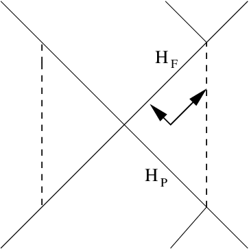
Thus, the only process potentially capable of modifying the singularity would be its conjectured screening by absorption of charged particles. Of course the mass inflation phenomenon is an issue here but, in the context of perfect spherical symmetry, exact solutions of the Einstein–Maxwell system exist having both event and Cauchy horizons and describing collapse of spherical shells. For these what we said should apply. The present formalism also predicts the absence of particle creation in the region in between the two horizons, despite the metric there is dynamical. The possibility that the naked singularity itself radiates away its mass will be taken up in the next section.
5.5 Naked singularities
A general reference on the physics of naked singularities is [186]. Particle emission from naked singularities in higher dimensions has been studied also in [187]. Sticking to two-dimensional models for simplicity, consider the following metric [188]
| (5.30) |
where is related to the cosmological constant by .
This metric arises as a solution of two-dimensional dilaton gravity coupled to a bosonic field with stress tensor , describing a shock wave. A look at fig.6 reveals that is a naked singularity partly to the future of a flat space region, usually named the linear dilaton vacuum. The heavy arrow represents the history of the shock wave responsible for the existence of the time-like singularity. The Hamilton–Jacobi equation implies either or , being the action. To find the ingoing flux we integrate along till we encounter the naked singularity, using , so that
| (5.31) |
where and is the familiar Kodama’s energy. The imaginary part immediately follows on using , giving the absorption probability as a function of retarded time
| (5.32) |
being some pre-factor of order one.
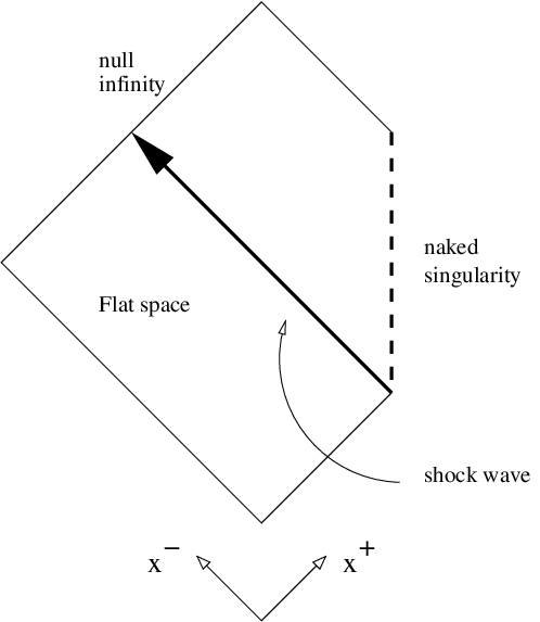
The flux is computed by integrating the probability over the coordinate frequency (that is, the variable conjugated to the coordinate time) , with the density of states measure , which gives
| (5.33) |
Similarly, in order to find the outgoing flux we integrate along starting from the naked singularity, this time using . A similar calculation gives
| (5.34) |
then, integrating the probability over the coordinate frequency, we obtain
| (5.35) |
The outgoing flux is . The conservation equations
| (5.36) |
determine the components only up to arbitrary functions and , something which corresponds to the freedom in the choice of a vacuum. For instance, requiring the fluxes to vanish in the linear dilaton vacuum fixes them uniquely. As it is well known, is given by the conformal anomaly: (for one bosonic degree of freedom). Matching to the anomaly gives the pre-factor , of order one indeed. These results agree with the one-loop calculation to be found in [188]. Note that the stress tensor diverges while approaching the singularity, indicating that its resolution will not be possible within classical gravity but requires quantum gravity instead [189, 190].
We return now to the Reissner–Nordström solution. Could it be that the naked singularity emits particles? In the four-dimensional case one easily sees that the action has no imaginary part along null trajectories either ending or beginning at the singularity. Formally this is because the Kodama energy coincides with the Killing energy in such a static manifold and there is no infinite red-shift from the singularity to infinity. Even considering the metric as a genuinely two-dimensional solution, this would lead to an integral for
| (5.37) |
where , with
| (5.38) |
But close to the singularity
| (5.39) |
not a simple pole, rather, an integrable singularity. It is fair to say that the Reissner–Nordström naked singularity will not emit particles in this approximation. This seems to be coherent with quantum field theoretical results. With the customary and , there is a map which gives the family of ingoing null geodesics, characterised by constant values of , which after reflection in the origin emerge as the the family of outgoing null geodesics with constant . According to [191], the radiated s-wave power of a minimally coupled scalar field is given in terms of the map by the Schwarzian derivative
| (5.40) |
The section of the Reissner–Nordström metric is conformally flat, hence the above map is trivial (i.e. linear) and .
6 Conclusions
We have completed our journey into the realm of quantum gravitational effects that can be understood as a result of tunnelling processes. In this journey, we visited black hole radiation, de Sitter and cosmological radiation, decays and naked singularities, but we have not included tunnelling between different gravitational field configurations, nor topology changing processes, nor sonic black holes or other analogue objects. Thus we may generically qualify the subject as covering semi-classical effects in a given background field. From this point of view it seemed remarkable that it could be extended to cover back-reaction effects to first order in the ratio , where is the energy scale of the tunnelling process and the black hole mass or some generalisation thereof. We would like to conclude by summarising the achievements, the drawbacks and the prospects.
Achievements. We list the results which seem to us more robust and have a chance to last longer. And also what is to be expected, reasonably, by pursuing this approach still further. Results that were obtained in Section 2 and Section 3 comprise:
- 1.
The ability of the method to include first order back-reaction effects in order to comply with energy conservation and the predicted correlations among successive emission events is one of the key results.
- 2.
In the stationary case, it is possible to provide a foundation of tunnelling methods using analytic continuation of the classical action alone, avoiding in this way the seemingly impossible task of crossing the horizon. The analytic continuation could be extended to cover white holes and to associate with them a well defined geometric temperature, a point not always appreciated in literature.
- 3.
In the same vein, one can prove the complete equivalence of the null geodesic method with the Hamilton–Jacobi method for stationary fields. We also gave a “covariantised” version of the null geodesic method, which allows to avoid questions such as covariance or canonical invariance.
- 4.
Many special cases have been considered, including rotating black holes, Gödel space-times, higher dimensional solutions, de Sitter and anti–de Sitter spaces, Taub and Taub–NUT solutions; also, we considered some supergravity solutions and fermion tunnelling, including gravitinos. The temperature of these solutions were computed and showed to agree with those obtained by geometric methods, confirming the universal character and kinematics of the Hawking effect. It should also be noticed that the Hawking temperature computed from the tunnelling method does not receive higher order corrections in , contrary to past suggestions.
In Section 4, using a local notion of horizon and dynamical surface gravity for time varying spherically symmetric black holes, the main results comprise:
- 1.
The application of the tunnelling method to non stationary, spherically symmetric black holes and the fact that it naturally selects a trapping horizon of the future non degenerate type, either inner or outer. It can also be applied to past horizons under the same condition and by interchanging emission with absorption. In the limiting situation where the surface gravity vanishes it is consistent with the idea that extremal black holes have zero temperature.
- 2.
One of the principal consequences of the tunnelling method is the observation that the radiation seems to originate near the local trapping horizon, not the global event horizon.
- 3.
Using the Kodama–Hayward theory of spherically symmetric space-times, and noting that one can possibly associate an observable temperature to a black hole only if it is a coordinate scalar, we showed that the tunnelling probability depends on the ratio, , of the Kodama invariant charge taken as energy and the geometrical surface gravity as defined by Hayward.
- 4.
One can include non interacting fermions in the formalism, as demonstrated in several papers. Also noticeable is the fact that any mass term gets strongly suppressed by the horizon pole, which dominates the rate well over mass contributions.
- 5.
The time-like nature of the trapping horizon of an excreting black hole is consistent with the physical interpretation of the formalism. It is true that it can be crossed either ways, but it remains the fact that there is a class of paths for which an imaginary part exists, and these paths precisely correspond in Feynman diagram language to particle creation.
In Section 5 we addressed other themes – cosmology, decays and naked singularities. Since FRW spaces are spherically symmetric, the general theory outlined in Section 4.2 applies. We showed that, with obvious modifications, the tunnelling picture works equally well. In particular the type-II paths never contribute, while type-I paths do. We may consider these findings for cosmological horizons as a generalisation of the well known facts discovered for de Sitter space-time, in complete analogy with the parallel extension of the theory from stationary to dynamical black holes. We also considered the decay of particles which in the absence of gravity would not occur, and find that the Hamilton–Jacobi equation can manage them through the presence of a branch point singularity in the radial momentum, that would not be present in absence of an external field. From this point of view the tunnelling method has universally valid features. Again, its value is to be found where it provides approximate results when exact calculations are in general impossible, at the same time being consistent with the exact calculations when available. Such is the case of de Sitter space. We showed also that the presence of strong fields in a certain space-time region, even in the absence of horizons, can result in particle production by means of a tunnelling process “from nothing”. It can be considered as the gravitational analogue of the Schwinger effect in a strong external electric field. Finally, it is of interest that the tunnelling method can also be applied to naked singularities, although in this case there is nothing to tunnel through, the singularity being the boundary of space-time. We showed nevertheless that the emerging picture is quite in agreement with quantum field theory in two-dimensional models, making one confident of its general validity.
As regard the drawbacks, in the stationary case one can perhaps complain that the method gives only approximate results. But for black holes with really intricate metrics exact calculations are illusory even in stationarity, so we feel that this is not a serious drawback. Even if there is little doubt that the method is correct, still it remains of a hypothetical nature. However, we think that also in case of a failure due to some internal inconsistency, that should be nonetheless an important message. In fact, tunnelling processes are predictions of quantum theory, so a failure of them in gravity theory would certainly signal something interesting. Despite all the desirable properties discussed above, the tunnelling method is and remains an essentially semi-classical procedure carrying along with it all the limitations inherent to its nature. In particular, it applies only to free particles while in principle quantum field theory methods certainly have a wider scope.
Prospects. The tunnelling method is not a closed subject. For instance, in striking contrast with the stationary case, an important missing point of the dynamical case is the absence of an extension of Kodama–Hayward’s theory to dynamical axis-symmetric black holes, to be used as a tool for studying tunnelling. We mention here the papers [192, 193] where a tentative theory is developed. We feel that this is perhaps the most important missing point. The first back-reaction corrections are also of great interest, as they are not so well developed in dynamical situations. Processes where small black holes are emitted by large ones should also be within the range of problems where the tunnelling picture could work, and that also is an important “to do”.
In cosmology, the physical interpretation of Hayward’s dynamical surface gravity as a temperature is not as clear as in de Sitter or black hole case, but it is strongly favoured by the tunnelling picture. In particular, an Unruh–DeWitt detector moving in de Sitter or black hole space-time always thermalises at the corresponding Gibbons–Hawking temperature even if it is not on a geodesic path, while for cosmology there is not an analogous result. One may conjecture that the cosmological temperature given by eq.(5.4 is the one that a point-like detector registers when moving on a Kodama trajectory, whose four-velocity is the Kodama vector field. In general, such a trajectory is accelerated relative to geodesic observers so one expects a mixed contribution from the horizon and the acceleration together. These expectations were actually confirmed years ago in de Sitter and anti–de Sitter space and resulted in beautiful formulas [194, 195]. It would be very interesting to apply tunnelling methods also to Unruh’s like detectors (but see [51]). Finally, two more intriguing prospects are the application to field theories where fields, rather than particles, tunnel across forbidden regions; and to sonic black holes [201], or dielectric black hole analogues [202], since both can be studied in laboratory experiments. But these arguments would easily cover another review.
References
- [1] Hawking S W 1974 Nature 248 30; Hawking S W 1975 Commun. Math. Phys. 43 199–220
- [2] Parentani R and Brout R 1992 Int. J. Mod. Phys. D 1 169–91
- [3] Brout R, Massar S, Parentani R and Spindel Ph 1995 Phys. Rept. 260 329–446
- [4] Traschen J H 2000 An introduction to black hole evaporation (Singapore: World Scientific)
- [5] Jacobson T 2003 Introduction to quantum fields in curved space-time and the Hawking effect Preprint gr-qc/0308048
- [6] Page D N 2005 New J. Phys. 7 203
- [7] ’t Hooft G 1993 Dimensional reduction in quantum gravity Preprint gr-qc/9310026; ’t Hooft G 1995 Nucl. Phys. Proc. Suppl. 43 1–11
- [8] Susskind L 1995 J. Math. Phys. 36 6377–96
- [9] Susskind L, Thorlacius L and Uglum J 1993 Phys. Rev. D 48 3743–61
- [10] Jacobson T 1993 Phys. Rev. D 48 728–41
- [11] Visser M 1998 Phys. Rev. Lett. 80 3436–9
- [12] Visser M 2003 Int. J. Mod. Phys. D 12 649
- [13] Barcelo C, Liberati S, Sonego S and Visser M 2006 Phys. Rev. Lett. 97 171301
- [14] Schutzhold R and Unruh W G 2008 Phys. Rev.D 78 041504
- [15] Kiefer C 2001 Class. Quantum Grav. 18 L151
- [16] Vaz C, Kiefer C, Singh T P and Witten L 2003 Phys. Rev.D 67 024014
- [17] Unruh W G and Schutzhold R 2005 Phys. Rev.D 71 024028
- [18] Kiefer C, Muller–Hill J, Singh T P and Vaz C 2007 Phys. Rev.D 75 124010
- [19] Gallo E and Marolf D 2009 Am. J. Phys. 77 294–307
- [20] Birrell N D and Davies P C W 1982 Quantum fields in curved space (Cambridge: Cambridge University Press)
- [21] Schutzhold R 2001 Phys. Rev.D 63 024014
- [22] DeWitt B S 1975 Phys. Rept. 19 295–357
- [23] Gibbons G W and Hawking S W 1977 Phys. Rev.D 15 2738–51
- [24] Damour T and Ruffini R 1976 Phys. Rev.D 14 332–4
- [25] Srinivasan K and Padmanabhan T 1999 Phys. Rev.D 60 24007
- [26] Shankaranarayanan S, Srinivasan K and Padmanabhan T 2001 Mod.Phys.Lett. A 16 571–8
- [27] Shankaranarayanan S, Padmanabhan T and Srinivasan K 2002 Class. Quantum Grav. 19 2671–88
- [28] Padmanabhan T 2004 Mod. Phys. Letts. A 19 2637–43
- [29] Massar S and Parentani R 2000 Nucl. Phys. B 575 333–56
- [30] Kraus P and Wilczek F 1995 Nucl. Phys. B 433 403–20
- [31] Kraus P and Wilczek F 1995 Nucl. Phys. B 437 231–42
- [32] Parikh M K and Wilczek F 2000 Phys. Rev. Lett. 85 5042–5
- [33] Kraus P 2007 Non-thermal aspects of black hole radiance Preprint gr-qc/9508007
- [34] Moretti V and Pinamonti N 2010 State independence for tunnelling processes through black hole horizons and Hawking radiation Preprint gr-qc/1011.2994
- [35] Hemming S and Keski–Vakkuri E 2001 Phys. Rev.D 64 044006
- [36] Volovik G E 2009 Int. J. Mod. Phys. D 18 1227–41
- [37] Parikh M K 2002 Phys. Lett. B 546 189
- [38] Medved A J M 2002 Phys. Rev.D 66 124009
- [39] Shankaranarayanan S 2003 Phys. Rev.D 67 084026; Wu S Q and Jiang Q Q 2006 Hawking Radiation of Charged Particles as Tunneling from Higher Dimensional Reissner–Nordström–de Sitter Black Holes Preprint hep-th/0603082; Sekiwa Y 2008 Decay of the cosmological constant by Hawking radiation as quantum tunneling Preprint hep-th/0802.3266; Chen D Y, Jiang Q Q and Zu X T 2008 Hawking radiation of Dirac particles via tunnelling from rotating black holes in de Sitter spaces Preprint hep-th/0804.0131
- [40] Stotyn S, Schleich K and Witt D 2009 Class. Quantum Grav. 26 065010
- [41] Zhang B, Cai Q, You L and Zhan M 2009 Phys. Lett. B 675 98–101
- [42] Zhang B, Cai Q, Zhan M and You L 2011 Annals Phys. 326 350–63
- [43] Israel W and Yun Z 2010 Phys. Rev.D 82 124036
- [44] Angheben M, Nadalini M, Vanzo L and Zerbini S 2005 JHEP 0505 014; Nadalini M, Vanzo L and Zerbini S 2006 J. Phys A 39 6601
- [45] Di Criscienzo R, Nadalini M, Vanzo L, Zerbini S and Zoccatelli G 2007 Phys. Lett. B 657 107–11
- [46] Kerner R and Mann R B 2006 Phys. Rev. D 73 104010
- [47] Chatterjee B, Ghosh A and Mitra P 2008 Phys. Lett. B 661 307–11
- [48] Kerner R and Mann R B 2007 Phys. Rev. D 75 084022
- [49] Nielsen A B and Visser M 2006 Class. Quantum Grav. 23 4637
- [50] Wu X-n and Gao S 2007 Phys. Rev.D 75 044027
- [51] de Gill A, Singleton D, Akhmedova V and Pilling T 2010 Am. J. Phys. 78 685–91
- [52] Frolov V P and Novikov I D 1998 Black Hole Physics. Basic Concepts and New Developments (Dordrecht: Kluwer Academic Publishers)
- [53] Parikh M K 2004 A Secret Tunnel Through The Horizon Preprint hep-th/0405160
- [54] Hartle J B and Hawking S W 1976 Phys. Rev. D 13 2188
- [55] Hawking S W and Ellis G F R 1973 The large scale structure of space-time (Cambridge: Cambridge University Press)
- [56] Painlevé P 1921 Compt. Rend. Acad. Sci. 173 677; Gullstrand A 1922 Arkiv. Mat. Astron. Fys. 16 1
- [57] Thomsen J S 1953 Phys. Rev.91 1263–6
- [58] Hawking S W 1971 Phys. Rev. Lett. 26 1344; Bekenstein J D 1972 Lett. Nuov. Cimento 4 737; Bekenstein J D 1973 Phys. Rev. D 7 2333–46
- [59] Landau L D and Lifshitz E M 1980 Course of Theoretical Physics. Vol. 5. Statistical Physics (Oxford: Pergamon Press)
- [60] Gibbons G W and Hawking S W 1977 Phys. Rev. D 15 2752–6
- [61] Parikh M K 2004 Energy conservation and Hawking radiation Preprint hep-th/0402166
- [62] Arzano M, Medved A J M and Vagenas E C 2005 JHEP 0509 037; Medved A J M and Vagenas E C 2005 Mod. Phys. Lett. A 20 1723–8
- [63] Mann R B and Ross S 1995 Phys. Rev. D 52 2254; Bousso R and Hawking S W 1996 Phys. Rev. D 54 6312
- [64] Di Criscienzo R, Hayward S, Nadalini M, Vanzo L and Zerbini S 2010 Class. Quantum Grav. 27 015006
- [65] Eddington A S 1924 Nature 113 192; Finkelstein D 1958 Phys. Rev. 110 965
- [66] Tolman R C 1934 Relativity, Thermodynamics and Cosmology (Oxford: Clarendon Press)
- [67] Visser M 1992 Phys. Rev. D 46 2445–51
- [68] Jacobson T 2007 Class. Quantum Grav. 24 5717–9
- [69] Di Criscienzo R, Hayward S A, Nadalini M, Vanzo L and Zerbini S 2010 Class. Quantum Grav.27 015006
- [70] Kerner R and Mann R B 2008 Class. Quantum Grav. 25 09501
- [71] Yale A 2011 Phys. Lett. B 697 398–403
- [72] Di Criscienzo R and Vanzo L 2008 Europhys. Lett. 82 60001
- [73] Li H L, Yang S Z, Zhou T J and Lin R 2008 Europhys. Lett. 84 20003
- [74] Kerner R and Mann R B 2008 Phys. Lett. B 665 4
- [75] Yale A and Mann RB 2009 Phys. Lett. B 673 168–72
- [76] Rehman M and Saifullah K 2011 JCAP 03 001
- [77] Chatterjee B and Mitra P 2009 Phys. Lett. B 675 240–2
- [78] Yale A 2011 Eur. Phys. J. C 71 1622
- [79] Banerjee R and Majhi B R 2008 JHEP 0806
- [80] Majhi B R 2009 Phys. Rev.D 79 044005
- [81] Majhi P R and Samanta S 2010 Annals Phys. 325 2410–24
- [82] Banerjee R, Kiefer C and Majhi B R 2010 Phys. Rev. D 82 044013
- [83] Banerjee R and Majhi B R 2009 Phys. Lett. B 675 243–5
- [84] Barducci A, Casalbuoni R and Lusanna L 1976 Nuovo Cimento A 35 377
- [85] Cognola G, Vanzo L, Zerbini S and Soldati R 1981 Phys. Lett. B 104 67–9
- [86] Berezin F A and Marinov M S 1977 Annals Phys. 104 336
- [87] Bardeen J M 1970 Nature 226 64
- [88] Tamburini F, Thide B, Molina–Terriza G and Anzolin G 2011 Nature Phys. Lett. 7 195–7
- [89] Kerr R P 1963 Phys. Rev. Lett. 11 237–8
- [90] Jiang Q Q, Wu S Q and Cai X 2006 Phys. Rev. D 73 064003
- [91] Angheben M, Nadalini M, Vanzo L and Zerbini S 2005 JHEP 0505 014
- [92] Brandt F 2002 Fortschr. Phys. 50 1126
- [93] Griffiths J B and Podolsky J 2005 Class. Quantum Grav. 22 3467
- [94] Podolsky J and Kadlecovà H 2009 Class. Quantum Grav. 26 105007
- [95] Gimon E G and Hashimoto A 2003 Phys. Rev. Lett. 91 021601
- [96] Myers R C and Perry M J 1986 Annals Phys. 172 304
- [97] Vanzo L and Klemm D 2005 Fortsch. Phys. 53 919–25
- [98] Astefanesei D, Mann R B and Radu E 2005 JHEP 01 049
- [99] Mann R B and Stelea C 2005 Phys. Rev. D 72 084032
- [100] Bañados M, Teitelboim C and Zanelli J 1992 Phys. Rev. Lett. 69 1849–51
- [101] Medved A J M 2002 Class. Quantum Grav. 19 589–98
- [102] Li R and Ren J R 2008 Phys. Lett. B 661 370–2
- [103] Åminneborg S, Bengtsson I, Holst S and Peldan P 1996 Class. Quantum Grav. 13 2707
- [104] Mann R B 1997 Class. Quantum Grav. 14 L109
- [105] Vanzo L 1997 Phys. Rev.D 56 6475–83
- [106] Brill D R, Louko J and Peldan P 1997 Phys. Rev.D 56 3600–10
- [107] Gibbons G W and Maeda K 1988 Nucl. Phys. B 298 741
- [108] Garfinkle D, Horowitz G T and Strominger A 1991 Phys. Rev. D 43 3140
- [109] Holzhey C F E and Wilczek F 1992 Nucl. Phys. B 380 447
- [110] Preskill J, Schwarz P, Shapere A D, Trivedi S and Wilczek F 1991 Mod. Phys. Lett. A 6 2353
- [111] Caldarelli M, Vanzo L and Zerbini S 2000 The Extremal limit of D-dimensional black holes Preprint hep-th/0008136
- [112] Nariai H 1951 Science Report of the Tohoku Univ. 35 62
- [113] Ginsparg P H and Perry M J 1983 Nucl. Phys. B 222 245
- [114] Bousso R 1997 Phys. Rev.D 55 3614–21
- [115] Gibbons G W 1975 Comm. Math. Phys. 44 245–64
- [116] Vanzo L 1997 Phys. Rev. D 55 2192–201
- [117] Wang W, Ding C, Chen S and Jing J 2010 Gen. Rel. Grav. 42 347–57
- [118] Vanzo L 2011 On tunneling across horizons Preprint gr-qc/1104.1569, in press on Europhysics Lett.
- [119] Wald R M 1984 General Relativity (Chicago: University of Chicago Press)
- [120] Pizzi M 2009 Second comment to “Invariance of the tunneling method” Preprint gr-qc/0909.3800; Hayward S A, Di Criscienzo R, Nadalini M, Vanzo L and Zerbini S 2009 Comment on “On the tunneling through the black hole horizon” Preprint gr-qc/0911.4417; Hayward S A, Di Criscienzo R, Nadalini M, Vanzo L and Zerbini S 2009 Reply to Comments on “Invariance of the tunneling method for dynamical black holes” Preprint gr-qc/0909.2956
- [121] Akhmedov E T, Akhmedova V and Singleton D 2006 Phys. Lett. B 642 124; Nakamura T K 2007 Factor Two Discrepancy of Hawking Radiation Temperature Preprint 0706.2916; Mitra P 2007 Phys. Lett. B 648 240
- [122] Mitra P 2007 Phys. Lett. B 648 240–2
- [123] Stotyn S, Schleich K and Witt D M 2009 Class. Quantum Grav. 26 065010
- [124] Bellini E, Di Criscienzo R, Sebastiani L and Zerbini S 2010 Entropy 12 2186–98
- [125] Akhmedov E T, Pilling T and Singleton D 2008 Int. J. Mod. Phys. D 17 2453–8
- [126] Chowdhury B D 2008 Pramana 70 3–26
- [127] Medved A J M and Vagenas E C 2005 Mod. Phys. Lett. A 20 2449–54
- [128] Vagenas E C 2003 Phys. Lett. B 559 65–73; Arzano M, Medved A J M and Vagenas E C 2005 JHEP 0509 037; Jiang Q Q, Li H L, Yang S Z and Chen D Y 2007 Mod. Phys. Lett. A 22 891
- [129] Yang S and Chen D 2007 Int. J. Theor. Phys. 46 1747–52
- [130] Vaidya P C 1951 Proc.Indian Acad. Sci. A 33 264; Vaidya P C 1953 Nature 171 260; Narlikar V V and Vaidya P C 1947 Nature 159 642
- [131] Bardeen J M 1981 Phys. Rev. Lett. 46 382
- [132] York J W 1983 Phys. Rev.D 28 2929
- [133] Booth I and Fairhurst S 2004 Phys. Rev. Lett. 92 011102
- [134] Brevik I 2000 Phys. Rev.D 61 124017
- [135] Nojiri S and Odintsov S D 2000 Int. J. Mod. Phys. A 15 989
- [136] Fredenhagen K and Haag R 1990 Commun. Math. Phys. 127 273
- [137] Hayward S A 1994 Phys. Rev.D 49 6467
- [138] Hayward S A 1994 Class. Quantum Grav. 11 3025
- [139] Hayward S A 1998 Class. Quantum Grav. 15 3147–62
- [140] Ashtekar A, Beetle C and Fairhurst S 1999 Class. Quantum Grav. 16 L1
- [141] Ashtekar A, Corichi A and Krasnov K 2000 Adv. Theor. Math. Phys. 3 419; Ashtekar A, Fairhurst S and Krishnan B 2000 Phys. Rev. D 62 104025; Ashtekar A, Beetle C, Dreyer O, Fairhurst S, Krishnan B, Lewandowski J and Wisniewski J 2000 Phys. Rev. Lett. 85 3564
- [142] Ashtekar A and Krishnan B 2002 Phys. Rev. Lett. 89 261101
- [143] Ashtekar A and Krishnan B 2003 Phys. Rev. D 68 104030
- [144] Ashtekar A and Krishnan B 2004 Living Rev. Rel. 7 10
- [145] Gourgoulhon E and Jaramillo J L 2008 New Astron. Rev. 51 791
- [146] Hájiček P 1973 Comm. Math. Phys. 34 37; Hájiček P 1977 Lett. Nuovo Cim. 18 251–4
- [147] Hayward S A 1994 Class. Quantum Grav. 11 3037–48
- [148] Hayward S A 1996 Phys. Rev.D 53 1938–49
- [149] Hayward S A 2004 Phys. Rev. Lett.93 251101; Hayward S A 2004 Phys. Rev.D 70 104027; Hayward S A 2006 Phys. Rev.D 74 104013
- [150] Ben–Dov I 2004 Phys. Rev.D 70 124031
- [151] Andersson L, Mars M and Simon W 2005 Phys. Rev. Lett. 95 111102
- [152] Hayward S A 2004 Phys. Rev.D 70 104027
- [153] Gourgoulhon E 2005 Phys. Rev. D 72 104007
- [154] Gourgoulhon E and Jaramillo J L 2006 Phys. Rev.D 74 087502
- [155] Nielsen A B and Yoon J H 2008 Class. Quantum Grav. 25 085010
- [156] Bardeen J M, Carter B and Hawking S W 1973 Commun. Math. Phys. 31 161
- [157] Fodor G, Nakamura K, Oshiro Y and Tomimatsu A 1996 Phys. Rev. D 54 3882
- [158] Kodama H 1980 Prog. Theor. Phys. 63 1217
- [159] Mukohyama S and Hayward S A 2000 Class. Quantum Grav. 17 2153
- [160] Vaidya P 1951 Proc. Indian Acad. Sci. A 33 264
- [161] Brown B A and Lindesay J 2010 AIP Conf. Proc. 1280 3–16
- [162] Lindesay J 2009 Class. Quantum Grav.26 125014
- [163] Lindesay J and Sheldon P 2010 Class. Quantum Grav.27 215015
- [164] Clifton T 2008 Class. Quantum Grav. 25 175022
- [165] McVittie G C 1933 Mon. Not. R. Astronomic Soc. 93 325
- [166] Nolan B C 1998 Phys. Rev.D 58 064006; Nolan B C 1999 Class. Quantum Grav.16 1227; Nolan B C 1999 Class. Quantum Grav.16 3183
- [167] Francis M R and Kosowsky A 2004 Am. J. Phys. 72 1204–9
- [168] Misner C W and Sharp D H 1964 Phys. Rev. 136 B571; Hawking S W 1968 J. Math. Phys. 9 598
- [169] Szabados L B 2004 Living Rev. Relativity 7 4
- [170] Faraoni V 2007 Phys. Rev.D 76 104042
- [171] Abreu G and Visser M 2010 Phys. Rev.D 82 044027
- [172] Belinski V A 2009 On the Tunnelling Through the Black Hole Horizon Preprint gr-qc/0910.3934
- [173] Hiscock W A 1981 Phys. Rev.D 23 2813
- [174] Balbinot R 1986 Phys. Rev.D 33 1611
- [175] Arzano M, Medved A J M and Vagenas E C 2005 JHEP 0509 037; Arzano M 2006 Mod. Phys. Lett. A 21 41–8; Cai R G, Cao L M and Hu Y P 2009 Class. Quantum Grav. 26 155018; Cai R G, Cao L M and Hu Y P 2008 JHEP 0808 090; Cai R G and Cao L M 2007 Nucl. Phys. B 785 135–48; Cai R G and Cao L M 2007 Phys. Rev. D 75 064008
- [176] Jiang K X, Ke S M, Peng D T and Feng J 2009 Chin. Phys. Lett. 26 070401; Yang J 2009 Int. J. Theor. Phys. 48 2592–8; Zhu T, Ren J R and Singleton D 2010 Int. J. Mod. Phys. D 19 159–69; Li R, Ren J R and Shi D F 2009 Phys. Lett. B 670 446–8
- [177] Volovik G E 2008 On de Sitter radiation via quantum tunneling Preprint gr-qc/0803.3367
- [178] Di Criscienzo R, Vanzo L and Zerbini S 2010 JHEP 1005 092
- [179] Wu X and Gao S 2007 Phys. Rev.D 75 044027–1
- [180] Mallet R L 1986 Phys. Rev.D 33 2201
- [181] Wu S F, Wang B, Yang G H and Zhang P M 2008 Class. Quantum Grav. 25 235018
- [182] Brout R, Horwitz G and Weil D 1987 Phys. Lett. B 192 318
- [183] Volovik G E 2009 JETP Lett. 90 1
- [184] Myhrvold N P 1983 Phys. Rev.D 28 2439
- [185] Bros J, Epstein H and Moschella U 2008 JCAP 0802 003; Bros J, Epstein H and Moschella U 2010 Annales Henri Poincaré 11 611–58; Bros J, Epstein H, Gaudin M, Moschella U and Pasquier V 2010 Commum. Math. Phys. 295 261–88
- [186] Harada T, Iguchi H and Nakao K I 2002 Prog. Theor. Phys. 107 449–524
- [187] Miyamoto U, Nemoto H and Shimano M 2010 Particle Creation by Naked Singularities in Higher Dimensions Preprint gr-qc/1012.2374
- [188] Vaz C and Witten L 1994 Phys. Lett. B 325 27
- [189] Harada T, Iguchi H, Nakao K I, Singh T P, Tanaka T and Vaz C 2001 Phys. Rev. D 64 041501
- [190] Iguchi H and Harada T 2001 Class. Quantum Grav. 18 3681
- [191] Ford L H and Parker L 1978 Phys. Rev. D 17 1485
- [192] Jing J and Wang Y 1996 Int. J. Theor. Phys. 35 1481–91
- [193] Yang X J, He H and Zhao Z 2003 Gen. Rel. Grav. 35 579–94; Chen D and Yang S 2007 Gen. Rel. Grav. 39 1503–15
- [194] Narnhofer H, Peter I and Thirring W E 1996 Int. J. Mod. Phys. B 10 1507–20
- [195] Deser S and Levin O 1997 Class. Quantum Grav. 14 L163–8; Deser S and Levin O 1998 Class. Quantum Grav. 15 L85–7; Deser S and Levin O 1999 Phys. Rev.D 59 064004
- [196] de Vries A and Schmidt–Kaler T 2002 Phys. Rev.D 65 104022; Rabinowitz M 1999 Phys. Essays 12 346–57; Rabinowitz M 2003 Consequences of gravitational tunneling radiation Preprint astro-ph/0302469; Flambaum V V 2004 Tunneling into black hole, escape from black hole, reflection from horizon and pair creation Preprint gr-qc/0408013; Xue S S 2005 Gen. Rel. Grav. 37 857–72; Sarkar S and Kothawala D 2008 Phys. Lett. B 659 683–7; Kim S P 2007 JHEP 0711 048; Kim S P 2010 JHEP 1009 054; Singleton D, Vagenas E C, Zhu T and Ren J R 2010 JHEP 1008 089; Mehdipour S H 2009 Int. J. Mod. Phys. A 24 5669–80; Banerjee R and Majhi B R 2008 Phys. Lett. B 662 62–5; Banerjee R, Majhi B R and Vagenas E C 2010 Phys. Lett. B 686 279–82; Jiang Q Q and Cai X 2010 JHEP 1011 066; Banerjee R and Majhi B R 2009 Phys. Lett. B 675 243–5; Carlip S 2009 Lect. Notes Phys. 769 89–123; Pilling T 2008 Phys. Lett. B 660 402–6; Chowdhury B D 2008 Pramana 70 593–612; Medved A J M and Vagenas E C 2005 Mod. Phys. Lett. A 20 1723–8; Yale A 2010 Thermodynamics of Constant Curvature Black Holes Through Semi-Classical Tunnelling Preprint 1012.2114; Jiang Q Q, Han Y and Cai X 2010 JHEP 1008 049; Zhang J and Zhao Z 2010 Discussion on Event Horizon and Quantum Ergosphere of Evaporating Black Holes in a Tunnelling Framework Preprint 1010.4085; Zhang B, Cai Q-y and Zhan M-s 2008 Phys. Lett. B 665 260–63; Zhang J Y and Zhao Z 2005 Phys. Lett. B 618 14–22; Ren J, Zhao Z and Gao C 2006 Gen. Relativ. Gravit. 38 387–92; Banerjee R, Majhi R B and Vagenas E C 2010 Europhys. Lett. 92 20001; Gao J, Luo Z Q, Liu W W and Li G 2010 Int. J. Theor. Phys. 49 1781–7; Dehghani M and Farmany A 2010 Int. J. Theor. Phys. 49 1633–40; Becar R, Gonzalez P, Pulgar G and Saavedra J 2010 Int. J. Mod. Phys. A 25 1463–75; Ding C, Wang M and Jing J 2009 Phys. Lett. B 676 99–104; Zhang B, Cai Q-y and Zhan M-s 2009 Phys. Lett. B 671 310–3; Zhang B, Cai Q-y and Zhan M-s 2010 Eur. Phys. J. C 68 561–6
- [197] Korkin R V and Khriplovich I B 2002 J. Exp. Theor. Phys. 94 453–8; Zhang J Y and Zhao Z 2005 JHEP 0510 055; Zhang J Y and Zhao Z 2005 Mod. Phys. Lett. A 20 1673–8; Zhang J Y and Zhao Z 2005 Nucl. Phys. B 725 173–80; Jiang Q Q and Wu S Q 2006 Phys. Lett. B 635 151–5; Li H L, Yang S Z, Jiang Q Q and Qi D J 2005 Nuovo Cimento B 120 1299–306; Zhao L 2005 Commun. Theor. Phys. 47 835–42; Ren J, Zheng Z and Gao C J 2006 Gen. Rel. Grav. 38 387–92; Xiang L and Shen Y G 2006 Int. J. Theor. Phys. 45 631–9; Liu C Z, Zhang J Y and Zhao Z 2006 Phys. Lett. B 639 670–4; Yang S Z, Jiang Q Q and Li H L 2006 Commun. Theor. Phys. 46 643–6; Li H L, Qi D J, Jiang Q Q and Yang S Z 2006 Int. J. Theor. Phys. 45 2471–9; Fang H-z 2007 Nucl. Phys. B 767 130–8; Li G Q 2007 Mod. Phys. Lett. A 22 209–12; Jiang Q Q 2008 Phys. Rev. D 78 044009; Chen D Y, Jiang Q Q and Zu X T 2008 Phys. Lett. B 665 106–10; Zeng X-x, Hao X-z and Yang S-z 2008 Int. J. Mod. Phys. D 17 2079–87; Li Q and Han Y W 2008 Int. J. Theor. Phys. 47 3248–56; Wang Q and Yang S Z 2008 Phys. Scripta 78 045003; Jiang Q Q 2008 Phys. Lett. B 666 517–21; Zeng X X and Yang S Z 2008 Gen. Rel. Grav. 40 2107–14; Lai X J, Zeng X X and Yang S Z 2008 Int. J. Theor. Phys. 47 2576–82; Chen D, Yang H and Zu X 2008 Eur. Phys. J. C 56 119–24; Chen D Y, Zu X T 2009 Mod. Phys. Lett. A 24 1159–65; Zeng X X, Li Q, Hao J B 2009 Int. J. Theor. Phys. 48 1090–7; Lin K and Yang S Z 2009 Chin. Phys. Lett. 26 010401; Ghosh T and SenGupta S 2011 Phys. Lett. B 696 167–72; Gillani U A, Rehman M and Saifullah K 2011 Hawking radiation of scalar particles from accelerating and rotating black holes Preprint 1102.0029; Dehghani M 2011 Int. J. Theor. Phys. 50 446–53; Li H L, Lin R and Wang C Y 2010 Commun. Theor. Phys. 54 849–53; Gillani U A and Saifullah K 2010 Tunneling of Dirac particles from accelerating and rotating black holes Preprint 1010.6106; Ren J R, Mao P J, Li R, Zhu T and Jia L Y 2010 Mod. Phys. Lett. A 25 2167–81; Umetsu K 2010 Phys. Lett. B 692 61–3; Wang G, Liu B and Liu W 2010 Gen. Rel. Grav. 42 633–40; Wang F J, Gui Y X and Ma C R 2007 Phys. Lett. B 650 317–20; Song S X, Huang J and Ren J R 2011 Astrophys. Space Sci. 331 145–9; Li R and Ren J R 2008 Class. Quantum Grav. 25 125016; Akhmedov E T, Akhmedova V, Pilling T and Singleton D 2007 Int. J. Mod. Phys. A 22 1705–15; Angheben M, Nadalini M, Vanzo L and Zerbini S 2005 JHEP 0505 014; He T M and Zhang J Y 2009 Commun. Theor. Phys. 52 619–21; Li H L 2010 Europhys. Lett. 92 20003
- [198] Medved A J M 2002 Class. Quantum Grav. 19 589–98; Vagenas E C 2002 Phys. Lett. B 533 302–6; Grumiller D and McNees R 2007 JHEP 0704 074; Ma Z Z 2008 Phys. Lett. B 666 376–81; Liu W 2008 Int. J. Theor. Phys. 47 1979–86; Chen D Y, Jiang Q Q and Zu X T 2008 Phys. Lett. B 665 106–10; Li R and Ren J R 2008 Phys. Lett. B 661 370–2; Nozari K and Mehdipour S H 2008 Class. Quantum Grav. 25 175015; Nozari K and Mehdipour S H 2009 JHEP 0903 061; Li H-l, Qi W-y and Lin R 2009 Phys. Lett. B 677 332–7; Zeng X-x 2009 Mod. Phys. Lett. A 24 625–32; Lin K and Yang S 2009 Phys. Lett. B 674 127–30; Wang Q, Lin K and Yang S-z 2009 Gen. Rel. Grav. 41 1887–93; Dehghani M 2010 Int. J. Theor. Phys. 49 2698–703; Chen D Y, Yang H and Zu X T 2009 Phys. Lett. B 681 463–8; Lin K and Yang S Z 2009 Phys. Rev.D 79 064035; Dehghani M and Farmany A 2009 Phys. Lett. B 675 460–2; Lin K and Yang S 2009 Phys. Lett. B 680 506–9; Li H L, Qi W Y and Lin R 2009 Phys. Lett. B 677 332–7; Jian Tand Bing-Bing C 2009 Acta Phys. Polon. B 40 241–50; Akbar M and Saifullah K 2010 Eur. Phys. J. C 67 205–11; Fang L 2010 Astrophys. Space Sci. 325 1–5; Matsuno K and Umetsu K 2011 Hawking radiation as tunnelling from squashed Kaluza–Klein black hole Preprint 1101.2091; Song S X, Huang J and Ren J R 2011 Astrophys. Space Sci. 331 145–9; Ghosh T and SenGupta S 2011 Phys. Lett. B 696 167–72; Li H L, Lin R and Wang C Y 2010 Commun. Theor. Phys. 54 849–53; Ma Z Z 2009 Class. Quantum Grav. 26 135003; Jiang J J, Meng Q M and Wang S 2009 Int. J. Theor. Phys. 48 2826–33
- [199] Xia J K, San–Min K and Dan–Tao P 2009 Int. J. Mod. Phys. D 18 1707–17; Acquaviva G, Di Criscienzo R, Vanzo L and Zerbini S 2011 Unruh–DeWitt detector and the interpretation of the horizon temperature in spherically symmetric dynamical space–times Preprint 1101.5254; Li H L and Yang S Z 2009 Chin. Phys. B 18 4721–5; Qi D J and Ru H Q 2011 Int. J. Theor. Phys. 50 269–74; Yang S Z, Lin K and Yang J 2009 Mod. Phys. Lett. A 24 2187–93; Lin K and Yang S 2009 Mod. Phys. Lett. A 24 1775–83; Di Criscienzo R, Hayward S A, Nadalini M, Vanzo L and Zerbini S 2010 Class. Quantum Grav. 27 015006; Siahaan H M and Triyanta 2010 Int. J. Mod. Phys. A 25 145–53; Vanzo L 2008 Some results on dynamical black holes Preprint 0811.3532; Zhou S and Liu W 2009 Mod. Phys. Lett. A 24 2099–106; Banerjee R and Modak S K 2009 JHEP 0911 073; Yang J and Yang S 2009 Phys. Scripta 80 015007; Lin K and Yang S Z 2009 Chin. Phys. B 18 2154–8; Li H L, Yang S Z, Zhou T J and Lin R 2008 Europhys. Lett. 84 20003
- [200] Zhu T and Ren J R 2009 Eur. Phys. J. C 62 413–8; Jiang K-x, Ke S-m, Peng D-t and Feng J 2009 Chin. Phys. Lett. 26 070401; Lin K and Yang S 2009 Int. J. Theor. Phys. 48 2061–7; Zhu T, Ren J R and Singleton D 2010 Int. J. Mod. Phys. D 19 159–69; Cai R G, Cao L M and Hu Y P 2009 Class. Quantum Grav. 26 155018; Zhu T, Ren J R and Li M F 2009 JCAP 0908 010; Li R, Ren J R and Shi D F 2009 Phys. Lett. B 670 446–8; Jiang K X, Feng T and Peng D T 2009 Int. J. Theor. Phys. 48 2112–21; Wei Y H 2010 Phys. Lett. B 689 129–32; Chen Y X and Shao K N 2010 Invariance of the Hamilton-Jacobi tunneling method for black holes and FRW model Preprint 1007.4367
- [201] Unruh W G 1981 Phys. Rev. Lett. 46 1351–3
- [202] Schutzhold R, Plunien G and Soff G 2002 Phys. Rev. Lett. 88 061101