跳到论文正文
W Papers独立论文阅读器 arXiv:1106.4020 论文正文 计算阅读时间 · 0%
引用这篇论文根据当前论文元数据生成,正式投稿前建议核对。


License: arXiv.org perpetual non-exclusive license
arXiv:1106.4020v1 [hep-ph] 20 Jun 2011

August 24, 2026

Minimal Lepton Flavor Violation and Renormalization Group Evolution of Lepton Masses and Mixing

Yuval Grossman Email: yg73@cornell.edu Affiliation: Institute for High Energy Phenomenology
Newman Laboratory of Elementary Particle Physics
Cornell University, Ithaca, NY 14853, USA
   Shamayita Ray Email: sr643@cornell.edu Affiliation: Institute for High Energy Phenomenology
Newman Laboratory of Elementary Particle Physics
Cornell University, Ithaca, NY 14853, USA
Abstract

We study the renormalization group equations (RGEs) of the neutrino parameters in models of Minimal Lepton Flavor Violation. In such models, the RGEs can be described in terms of flavor spurions, such that only the coefficients depend on the specific model. We explicitly demonstrate this method for the SM and MSSM for both Type-I and Type-III seesaw models. For that purpose, the RGEs of neutrino parameters in the MSSM Type-III seesaw have been computed. We have extended this method to get the evolution equations at second order. The implications for leptogenesis are also discussed.

I Introduction

The data from past and ongoing neutrino oscillation experiments, as well as from cosmology and astrophysics, have now confirmed that neutrinos have distinct masses and that the three neutrino flavors νe\nu_{e}, νμ\nu_{\mu} and ντ\nu_{\tau} mix among themselves to form the three mass eigenstates. The fact that the neutrinos are massive and mix implies non-conservation of lepton flavor. Hence, lepton flavor violating processes are expected in the lepton sector just as quark flavor violating processes arise in the quark sector.

In the quark sector of the Standard Model (SM), flavor violation is induced by the Yukawa matrices such that baryon number remains an exact symmetry. The fact that flavor changing neutral currents (FCNCs) are heavily suppressed puts stringent constraints on the possible structure of new degrees of freedom carrying flavor quantum numbers. These constraints can be satisfied either if new particles are very heavy or if flavor symmetries suppress the flavor changing couplings. One of the most predictive and restrictive symmetry principles that can be used is Minimal Flavor Violation (MFV) [1]. The MFV framework is the assumption that in the quark sector the only sources of flavor symmetry breaking are the Yukawa couplings.

While the idea of MFV has a straightforward and unique realization in the quark sector, the situation is different in the lepton sector. The reason is that the neutrinos can be Majorana particles, in which case total lepton number is no longer a symmetry of the theory. Due to this complication, the Minimal Lepton Flavor Violation (MLFV) hypothesis is not uniquely defined; there are two ways to define it [2]. In the first case, known as MLFV with minimal field content, we do not add any new field to the theory, and treat the neutrino mass terms as non-renormalizable terms. The only irreducible sources of lepton flavor violation are the charged-lepton Yukawa matrix and the effective left-handed Majorana mass matrix. The breaking of total Lepton Number (LN) is independent of the flavor violation and happens at some very high scale.

The other possibility, called MLFV with extended field contents (MLFV-ex), is to introduce new fields to the SM. In particular, three heavy right-handed neutrinos are added to the SM. Their Majorana mass term, which is assumed to be flavor universal, explicitly breaks LN. In this scenario, the two Yukawa matrices act as the only irreducible sources of flavor violation. In the MLFV-ex scenario, the low energy observables depend on the high energy parameters of the theory. For example, the FCNC constraints in the leptonic sector affects leptogenesis. This has been studied in [3] with the mass-splitting of the right-handed neutrinos, required for successful leptogenesis, being introduced from flavor symmetry considerations only. To have a complete understanding of the relation between the high energy parameters and the low energy observables, one needs to study the complete renormalization group (RG) evolution effects in this context. RG evolution has already been shown to have strong effects on leptogenesis [4]. Ref. [5] shows the stability of the MLFV under RG evolution in the context of soft masses in the Minimal Supersymmetric Standard Model (MSSM). While [6] takes into account the RG evolution effects in the context of μ→3​e\mu\to 3e and τ→3​ℓ\tau\to 3\ell decays, a general analysis of RG evolution of lepton masses and mixing parameters in the MLFV framework is still lacking.

In this paper, we consider the RG evolution of lepton masses and mixing parameters in the MLFV-ex scenario, with the SM as the low energy effective theory. The basic idea is that the RGEs can be written in terms of spurions that depend only on the Yukawa matrices. The coefficient of each term can be model dependent. Moreover, we assume that the universality of the Majorana masses is broken slightly, and hence treat the Majorana mass matrix as a spurion of our theory, and we get the RGE for this spurion as well. This is, in fact, a natural assumption as the universality is automatically broken in course of RG evolution. We show explicitly how one can write the RGEs for the SM and MSSM in both Type-I and Type-III seesaw models. The advantage of the spurion formalism is that it shows how each combination enters and can be used as a check for any MLFV model.

II The Model: ν\nuMSM and MLFV with extended field content

We consider the SM extended by three right-handed neutrinos, which are singlets under the SM gauge group. This model is referred to as the ν\nuMSM [7]. We also consider the case where they are triplet under the SU(2)L group later in this section.

We begin by considering the model excluding all mass terms of the leptons and gradually introduce mass terms to study their effect on the flavor symmetries of the theory, at different energy scales μ\mu. In the massless lepton limit, at high scale μ>MR\mu>M_{R}, the ν\nuMSM enjoys a flavor symmetry GLF0{\rm G}_{\rm{LF}}^{0}, similar to that of the quark sector, given by

GLF0=SU​(3)lL⊗SU​(3)eR⊗SU​(3)νR.{\rm G}_{\rm{LF}}^{0}={\rm{SU}}(3)_{l_{L}}\otimes{\rm{SU}}(3)_{e_{R}}\otimes{\rm{SU}}(3)_{\nu_{R}}\;. (1)

Here we consider only the non-Abelian part of the flavor symmetry group. This sector is also invariant under U(1) of hypercharge (YY), total lepton number (LN), as well as U(1)E (or U(1)ν), which corresponds to a rotation of the eRe_{R} (or νR\nu_{R}) fields.

The presence of Majorana mass term for the right-handed neutrinos reduces the symmetry. Let us denote the right-handed neutrinos by νRi\nu_{R}^{i}, i∈{1,2,3}i\in\{1,2,3\}. The only source of LN violation in this model is the Majorana mass term of these right-handed neutrinos given by

ℒMaj=−12​ν¯RC​Mν​νR+h.c.,\displaystyle{\cal L}_{\rm Maj}=-\frac{1}{2}\bar{\nu}_{R}^{C}M_{\nu}\nu_{R}+{\rm{h.c.}}\;, (2)

where CC denotes charge conjugation. The right-handed Majorana mass matrix MνM_{\nu} is symmetric, Mν=MνTM_{\nu}=M_{\nu}^{T}. Furthermore, without any loss of generality, we can choose MνM_{\nu} to be real by re-definition of the phases of νRi\nu_{R}^{i}. (The ν\nuMSM was originally defined [7] in the basis where the charged lepton mass matrix and the Majorana mass matrix are real and diagonal.) In general MνM_{\nu} breaks SU​(3)νR{\rm{SU}}(3)_{\nu_{R}} completely. For a universal mass matrix, however, the breaking is into an O(3) group. In this case, the Majorana mass matrix is given by

(Mν)i​j=MR​δi​j,\left(M_{\nu}\right)_{ij}=M_{R}\delta_{ij}\;, (3)

and the flavor symmetry group becomes

GLF0→GLF=SU​(3)lL⊗SU​(3)eR⊗O​(3)νR.{\rm G}_{\rm{LF}}^{0}\to{\rm G}_{\rm{LF}}={\rm{SU}}(3)_{l_{L}}\otimes{\rm{SU}}(3)_{e_{R}}\otimes{\rm O}(3)_{\nu_{R}}\;. (4)

The two Yukawas YeY_{e} and YνY_{\nu} are given by

ℒYukawa=−e¯R​Ye​ϕ†​lL−ν¯R​Yν​ϕ~†​lL+h.c.,\displaystyle{\cal L}_{\rm Yukawa}=-\bar{e}_{R}Y_{e}\phi^{\dagger}l_{L}-\bar{\nu}_{R}Y_{\nu}{\widetilde{\phi}}^{\dagger}l_{L}+{\text{h.c.}}\;, (5)

where ϕ\phi is the SM Higgs doublet and ϕ~=i​σ2​ϕ∗\widetilde{\phi}=i\sigma^{2}\phi^{\ast}, σ2\sigma^{2} being the second Pauli matrix.

It is customary to treat GLF{\rm G}_{\rm{LF}} as an unbroken symmetry of the underlying theory which can be achieved by treating the Yukawa matrices as spurion fields with non-trivial quantum numbers under GLF{\rm G}_{\rm{LF}}

Ye∼(3¯,3,1),Yν∼(3¯,1,3).Y_{e}\sim(\bar{3},3,1)\;,\quad\quad Y_{\nu}\sim(\bar{3},1,3)\;. (6)

The ν\nuMSM in the massless lepton limit and with universal right-handed Majorana masses enjoys the flavor symmetry GLF{\rm G}_{\rm{LF}} and this is the MLFV hypothesis with extended field content (MLFV-ex) [2]. Going beyond the MLFV-ex hypothesis, in this paper we choose the universality of MνM_{\nu} to be slightly broken, which happens also as a result of RG evolution. We thus treat MνM_{\nu} as a spurion transforming, under GLF{\rm G}_{\rm{LF}}, as

Mν∼(1,1,6).M_{\nu}\sim(1,1,6)\;. (7)

The spurions have the following transformation properties:

Ye→UR​Ye​UL†,Yν→Oν​Yν​UL†,Mν→Oν​Mν​OνT,\displaystyle Y_{e}\to U_{R}Y_{e}U_{L}^{\dagger}\;,\qquad Y_{\nu}\to O_{\nu}Y_{\nu}U_{L}^{\dagger}\;,\qquad M_{\nu}\to O_{\nu}M_{\nu}O_{\nu}^{T}\;, (8)

where UL∈SU​(3)lLU_{L}\in{\rm{SU}}(3)_{l_{L}}, UR∈SU​(3)eRU_{R}\in{\rm{SU}}(3)_{e_{R}} and Oν∈O​(3)νRO_{\nu}\in{\rm O}(3)_{\nu_{R}}. This technique is known as spurion analysis.

Finally, the heavy fields generate small neutrino masses via the seesaw relation [8]

mν=v22​YνT​Mν−1​Yν,m_{\nu}=\frac{v^{2}}{2}Y_{\nu}^{T}M_{\nu}^{-1}Y_{\nu}\;, (9)

where the vacuum expectation value of the SM Higgs is defined as ⟨ϕ⟩=(0,v/2)T\langle\phi\rangle=(0,v/\sqrt{2})^{T}. In the MLFV-ex model, the left-handed neutrino mass matrix is given by

mν|MLFV−ex=v22​MR​YνT​Yν.\left.m_{\nu}\right\arrowvert_{\rm MLFV-ex}=\frac{v^{2}}{2M_{R}}Y_{\nu}^{T}Y_{\nu}\;. (10)

Note that in general YνT​YνY_{\nu}^{T}Y_{\nu} and Yν†​YνY_{\nu}^{\dagger}Y_{\nu} are two different sources of GLF{\rm G}_{\rm{LF}} breaking. Only in the limit where YνY_{\nu} is real are they the same [2]. We do, however, expect to have CP violation in the theory and thus we do not concentrate on the case of real YνY_{\nu}. We consider the MLFV-ex model for μ>MR\mu>M_{R} energy regime for the rest of the paper, with the exception that the universality of MνM_{\nu} is assumed to be slightly broken. We consider the case where MRM_{R} is large compared to the electroweak symmetry breaking scale. This ensures that U(1)LN is broken at some high scale, and that, in general, the breaking of LN by the Majorana mass term is independent of GLF{\rm G}_{\rm{LF}}-violation.

Next, we discuss the effective theory below MRM_{R}, or equivalently below the scale of the lightest of the heavy right-handed neutrinos, when universality is broken. In this regime, all the three heavy right-handed neutrinos get integrated out, and as a result the flavor symmetry group reduces to

GLF→GLF′=SU​(3)lL⊗SU​(3)eR.{\rm G}_{\rm{LF}}\to{\rm G}_{\rm{LF}}^{\prime}={\rm{SU}}(3)_{l_{L}}\otimes{\rm{SU}}(3)_{e_{R}}\;. (11)

In this energy region, the dimension-5 non-renormalizable term in the Lagrangian responsible for the LN-violating left-handed Majorana neutrino masses is of the form

ℒ∼l¯LC​mν​lL​ϕ​ϕ.{\cal L}\sim\bar{l}_{L}^{C}m_{\nu}l_{L}\phi\phi\;. (12)

There are two sources of GLF′{\rm G}_{\rm{LF}}^{\prime} breaking in this case. The charged lepton Yukawa YeY_{e} and the left-handed neutrino mass mνm_{\nu} that transform as

Ye∼(3¯,3),mν∼(6,1).Y_{e}\sim(\bar{3},3)\;,\quad m_{\nu}\sim(6,1)\;. (13)

Thus, the model becomes equivalent to the MLFV hypothesis with minimal field content [2]. In this case, mνm_{\nu} remains the only relevant quantity that contains the high energy information of the neutrino parameters, which in turn can be extracted by the measurement of the neutrino masses and mixing parameters. Hence, the effect of RG evolution becomes an important factor to be taken into account, which we will be studying in the following sections.

In the framework of spurion analysis, GLF{\rm G}_{\rm{LF}} is broken by the background values of the spurions. We consider the background values of Ye,νY_{e,\nu} to be small, the largest one being experimentally measured to be Yτ∼0.01Y_{\tau}\sim 0.01 at the scale MZM_{Z}. Thus, we can use perturbation theory and consider only the leading order corrections. To first order, the operators responsible for the breaking of GLF{\rm G}_{\rm{LF}} are combinations of two Yukawa matrices, that is, working at one loop is equivalent of considering spurions with two couplings. There are several combinations of couplings that can appear in the result. These couplings and their transformation properties are given in Table 1. As can be seen, MνM_{\nu} appears only when we consider the evolution of MνM_{\nu} itself.

Combination of spurions Transformation
Ye†​YeY_{e}^{\dagger}Y_{e} (8⊕1,1,1)(8\oplus 1,1,1)
Ye​Ye†Y_{e}Y_{e}^{\dagger} (1,8⊕1,1)(1,8\oplus 1,1)
Yν†​YνY_{\nu}^{\dagger}Y_{\nu} (8⊕1,1,1)(8\oplus 1,1,1)
Yν​Yν†Y_{\nu}Y_{\nu}^{\dagger} (1,1,8⊕1)(1,1,8\oplus 1)
Tr⁡[Ye†​Ye]=Tr⁡[Ye​Ye†]{\rm{Tr}}[Y_{e}^{\dagger}Y_{e}]={\rm{Tr}}[Y_{e}Y_{e}^{\dagger}] (1,1,1)(1,1,1)
Tr⁡[Yν†​Yν]=Tr⁡[Yν​Yν†]{\rm{Tr}}[Y_{\nu}^{\dagger}Y_{\nu}]={\rm{Tr}}[Y_{\nu}Y_{\nu}^{\dagger}] (1,1,1)(1,1,1)
Te≡Ye†​Ye−13​Tr​[Ye†​Ye]​𝐈3T_{e}\equiv Y_{e}^{\dagger}Y_{e}-\frac{1}{3}{\rm{Tr}}[Y_{e}^{\dagger}Y_{e}]{\mathbf{I}}_{3} (8,1,1)(8,1,1)
Te′≡Ye​Ye†−13​Tr​[Ye​Ye†]​𝐈3T_{e}^{\prime}\equiv Y_{e}Y_{e}^{\dagger}-\frac{1}{3}{\rm{Tr}}[Y_{e}Y_{e}^{\dagger}]{\mathbf{I}}_{3} (1,8,1)(1,8,1)
Tν≡Yν†​Yν−13​Tr​[Yν†​Yν]​𝐈3T_{\nu}\equiv Y_{\nu}^{\dagger}Y_{\nu}-\frac{1}{3}{\rm{Tr}}[Y_{\nu}^{\dagger}Y_{\nu}]{\mathbf{I}}_{3} (8,1,1)(8,1,1)
Tν′≡Yν​Yν†−13​Tr​[Yν​Yν†]​𝐈3T_{\nu}^{\prime}\equiv Y_{\nu}Y_{\nu}^{\dagger}-\frac{1}{3}{\rm{Tr}}[Y_{\nu}Y_{\nu}^{\dagger}]{\mathbf{I}}_{3} (1,1,8)(1,1,8)
Table 1: Transformations of combinations of two spurion fields under GLF{\rm G}_{\rm{LF}}. We have used the SU⁡(3){\rm{SU}}(3) algebra 3⊗3¯=8⊕13\otimes\bar{3}=8\oplus 1.

The flavor symmetry structure is more complicated when the heavy neutrinos are not exactly degenerate. A breaking of the universality of MνM_{\nu}, however small, is also necessary for leptogenesis as has been shown in [3]. In that paper, the degeneracy is broken by appropriate combinations of spurions in the MLFV-ex scenario. Our assumption is that the amount of non-degeneracy is small and GLF{\rm G}_{\rm{LF}} is still the flavor symmetry of the underlying theory. The effect of the breaking is due to the fact that running at the scale in between the three masses is not described by any of the two regions we discussed above. Yet, if the breaking is small this running is not significant and integrating out all the neutrinos together is a good approximation. Moreover, if the degeneracy is lifted due to RG evolution, then taking it into account is formally a higher order effect.

III RG evolution of neutrino parameters

We now study the effect of RG running. At energy scales above MRM_{R}, the quantities of interest are the Yukawa matrices Ye,νY_{e,\nu}, and the right-handed neutrino mass matrix MνM_{\nu}. Below, we see how they run.

In all our discussions, we consider only one loop running. In term of spurions, each loop add two Yukawa terms, and thus working at one loop is done by using only terms that have two Yukawa couplings more than the tree level one. The evolution equations at second order are discussed in Appendix B.

III.1 RG evolution of YeY_{e}

We define

Y˙e≡d​Yed​t,t≡ln⁡(μ/μ0)16​π2.\dot{Y}_{e}\equiv\frac{dY_{e}}{dt}\;,\qquad t\equiv\frac{\ln{(\mu/\mu_{0})}}{16\pi^{2}}\;. (14)

Here μ0(>MR)\mu_{0}(>M_{R}) is some high energy scale at which we start running and the factor (16​π2)(16\pi^{2}) appears because of the fact that we consider radiative corrections at 1-loop.

Under the flavor symmetry group GLF{\rm G}_{\rm{LF}}, YeY_{e} transforms as (3¯,3,1)(\bar{3},3,1) and so does Y˙e\dot{Y}_{e}. Hence Y˙e\dot{Y}_{e} can be expressed as appropriate combinations of the spurion fields transforming as (3¯,3,1)(\bar{3},3,1). Table 1 shows the combinations of two spurion fields with their transformation properties. Using the SU⁡(3){\rm{SU}}(3) algebra

8⊗3¯=15¯⊕6⊕3¯,8⊗3=15⊕6¯⊕3,8\otimes\bar{3}=\overline{15}\oplus 6\oplus\bar{3}\;,\qquad 8\otimes 3=15\oplus\bar{6}\oplus 3\;, (15)

and we can write

Ye​Te\displaystyle Y_{e}T_{e} =\displaystyle= (3¯,3,1)⊗(8,1,1)∋(3¯,3,1),\displaystyle(\bar{3},3,1)\otimes(8,1,1)\ni(\bar{3},3,1)\;, (16)
Ye​Tν\displaystyle Y_{e}T_{\nu} =\displaystyle= (3¯,3,1)⊗(8,1,1)∋(3¯,3,1),\displaystyle(\bar{3},3,1)\otimes(8,1,1)\ni(\bar{3},3,1)\;, (17)
Ye​Tr​[Ye†​Ye]\displaystyle Y_{e}{\rm{Tr}}[Y_{e}^{\dagger}Y_{e}] =\displaystyle= (3¯,3,1)⊗(1,1,1)=(3¯,3,1),\displaystyle(\bar{3},3,1)\otimes(1,1,1)=(\bar{3},3,1)\;, (18)
Ye​Tr​[Yν†​Yν]\displaystyle Y_{e}{\rm{Tr}}[Y_{\nu}^{\dagger}Y_{\nu}] =\displaystyle= (3¯,3,1)⊗(1,1,1)=(3¯,3,1).\displaystyle(\bar{3},3,1)\otimes(1,1,1)=(\bar{3},3,1)\;. (19)

The above combinations are the only terms, containing three spurion fields, allowed to appear on the right-hand side (RHS) of the RGE for Y˙e\dot{Y}_{e}. Te′​YeT_{e}^{\prime}Y_{e} gives the same term as that given by Ye​TeY_{e}T_{e} and so has not been listed separately. Thus, at 1-loop, when terms up to combinations of three spurion fields are allowed, the most general form of Y˙e\dot{Y}_{e} is given by

Y˙e\displaystyle\dot{Y}_{e} =\displaystyle= a1~​Ye​Te+a2~​Ye​Tν+a3~​Ye​Tr​[Ye†​Ye]+a4~​Ye​Tr​[Yν†​Yν]+a5​Ye\displaystyle\widetilde{a_{1}}Y_{e}T_{e}+\widetilde{a_{2}}Y_{e}T_{\nu}+\widetilde{a_{3}}Y_{e}{\rm{Tr}}[Y_{e}^{\dagger}Y_{e}]+\widetilde{a_{4}}Y_{e}{\rm{Tr}}[Y_{\nu}^{\dagger}Y_{\nu}]+a_{5}Y_{e} (20)
=\displaystyle= Ye​(a1​Ye†​Ye+a2​Yν†​Yν+a3​Tr​[Ye†​Ye]+a4​Tr​[Yν†​Yν]+a5​𝟙3),\displaystyle Y_{e}\left(a_{1}Y_{e}^{\dagger}Y_{e}+a_{2}Y_{\nu}^{\dagger}Y_{\nu}+a_{3}{\rm{Tr}}[Y_{e}^{\dagger}Y_{e}]+a_{4}{\rm{Tr}}[Y_{\nu}^{\dagger}Y_{\nu}]+a_{5}{\mathbbm{1}}_{3}\right)\;,

where a1a_{1}, a2a_{2}, a3a_{3}, a4a_{4} and a5a_{5} are expected to be numbers of 𝒪⁡(1){\cal O}(1) that can be determined by the calculation of the 1-loop diagrams in the theory.

The case of a5a_{5} is a bit more involved since it is a function independent of spurion fields. Thus a5a_{5} must contain combinations of other couplings in the theory that transform trivially under GLF{\rm G}_{\rm{LF}}. The couplings that we have in the theory are the gauge couplings, gig_{i}, the Higgs self-coupling, λ\lambda, and the quark Yukawa couplings YU,DY_{U,D}. Since leptons are singlets under SU​(3)C{\rm{SU}}(3)_{C}, g3g_{3} cannot contribute. Moreover, at 1-loop the Higgs self-coupling cannot contribute either. Terms proportional to g1g_{1} and g2g_{2} contributing to a5a_{5} must be of form

ag1​g12+ag2​g22.a_{g_{1}}g_{1}^{2}+a_{g_{2}}g_{2}^{2}\;. (21)

The singlet combination made of the quark Yukawas YU,DY_{U,D} is of the form Tr⁡[Yi†​Yi]{\rm{Tr}}[Y_{i}^{\dagger}Y_{i}], and the most general form of the quark Yukawa contributions to a5a_{5} is

aU​Tr​[YU†​YU]+aD​Tr​[YD†​YD].a_{U}{\rm{Tr}}[Y_{U}^{\dagger}Y_{U}]+a_{D}{\rm{Tr}}[Y_{D}^{\dagger}Y_{D}]. (22)

Thus the general form of a5a_{5} is given by

a5=ag1​g12+ag2​g22+aU​Tr​[YU†​YU]+aD​Tr​[YD†​YD],a_{5}=a_{g_{1}}g_{1}^{2}+a_{g_{2}}g_{2}^{2}+a_{U}{\rm{Tr}}[Y_{U}^{\dagger}Y_{U}]+a_{D}{\rm{Tr}}[Y_{D}^{\dagger}Y_{D}]\;, (23)

and the general form of Y˙e\dot{Y}_{e} becomes

Y˙e\displaystyle\dot{Y}_{e} =\displaystyle= Ye​(a1​Ye†​Ye+a2​Yν†​Yν)+Ye​(ag1​g12+ag2​g22)\displaystyle Y_{e}\left(a_{1}Y_{e}^{\dagger}Y_{e}+a_{2}Y_{\nu}^{\dagger}Y_{\nu}\right)+Y_{e}\left(a_{g_{1}}g_{1}^{2}+a_{g_{2}}g_{2}^{2}\right) (24)
+\displaystyle+ Ye​(a3​Tr​[Ye†​Ye]+a4​Tr​[Yν†​Yν]+aU​Tr​[YU†​YU]+aD​Tr​[YD†​YD]).\displaystyle Y_{e}\left(a_{3}{\rm{Tr}}[Y_{e}^{\dagger}Y_{e}]+a_{4}{\rm{Tr}}[Y_{\nu}^{\dagger}Y_{\nu}]+a_{U}{\rm{Tr}}[Y_{U}^{\dagger}Y_{U}]+a_{D}{\rm{Tr}}[Y_{D}^{\dagger}Y_{D}]\right)\;.

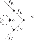
Terms proportional to Tr⁡[Yx†​Yx]{\rm{Tr}}[Y_{x}^{\dagger}Y_{x}] (x∈{e,ν,U,D}x\in\{e,\nu,U,D\}) arise from a complete fermion loop in the self-energy correction of the scalar Higgs boson, as shown in Fig. 1. Since quarks come in three colors, one gets

a3:a4:aU:aD=1:r:3:3,a_{3}:a_{4}:a_{U}:a_{D}=1:r:3:3, (25)

where each of the three quark colors contributes equally. r≡a4/a3r\equiv a_{4}/a_{3} is determined by the transformation properties of the right-handed neutrinos under the gauge group. As we discuss below, at Eq. (57), for singlets r=1r=1, while for triplets r=3r=3. We can now define a quantity

T≡Tr⁡[Ye†​Ye]+r​Tr​[Yν†​Yν]+3​T​r​[YU†​YU]+3​T​r​[YD†​YD],\displaystyle T\equiv{\rm{Tr}}[Y_{e}^{\dagger}Y_{e}]+r{\rm{Tr}}[Y_{\nu}^{\dagger}Y_{\nu}]+3{\rm{Tr}}[Y_{U}^{\dagger}Y_{U}]+3{\rm{Tr}}[Y_{D}^{\dagger}Y_{D}]\;, (26)

and write Y˙e\dot{Y}_{e} in a simpler form as

Y˙e\displaystyle\dot{Y}_{e} =\displaystyle= Ye​(a1​Ye†​Ye+a2​Yν†​Yν)+Ye​(aT​T+ag1​g12+ag2​g22),\displaystyle Y_{e}\left(a_{1}Y_{e}^{\dagger}Y_{e}+a_{2}Y_{\nu}^{\dagger}Y_{\nu}\right)+Y_{e}\left(a_{T}T+a_{g_{1}}g_{1}^{2}+a_{g_{2}}g_{2}^{2}\right)\;, (27)

where aTa_{T}, ag1a_{g_{1}}, ag2a_{g_{2}}, are expected to be of 𝒪⁡(1){\cal O}(1).

Refer to caption
Figure 1: The self-energy diagram of the Higgs ϕ\phi with complete fermion loop, where the fermion pair {fL,fR}\{f_{L},f_{R}\} can be {lL,eR}\{l_{L},e_{R}\}, {lL,νR}\{l_{L},\nu_{R}\}, {qL,uR}\{q_{L},u_{R}\} or {qL,dR}\{q_{L},d_{R}\} producing contributions proportional to Tr⁡[Ye†​Ye]{\rm{Tr}}[Y_{e}^{\dagger}Y_{e}], Tr⁡[Yν†​Yν]{\rm{Tr}}[Y_{\nu}^{\dagger}Y_{\nu}], Tr⁡[YU†​YU]{\rm{Tr}}[Y_{U}^{\dagger}Y_{U}] and Tr⁡[YD†​YD]{\rm{Tr}}[Y_{D}^{\dagger}Y_{D}] respectively.

III.2 RG evolution of YνY_{\nu}

Next, we discuss the running of YνY_{\nu}. Since YνY_{\nu} transforms as (3¯,1,3)(\bar{3},1,3) under GLF{\rm G}_{\rm{LF}}, so must be Y˙ν\dot{Y}_{\nu}. From Table 1 and using Eq. (15) we obtain that the only allowed combinations of spurion fields at one loop order are

Yν​Te\displaystyle Y_{\nu}T_{e} =\displaystyle= (3¯,1,3)⊗(8,1,1)∋(3¯,1,3),\displaystyle(\bar{3},1,3)\otimes(8,1,1)\ni(\bar{3},1,3)\;, (28)
Yν​Tν\displaystyle Y_{\nu}T_{\nu} =\displaystyle= (3¯,1,3)⊗(8,1,1)∋(3¯,1,3),\displaystyle(\bar{3},1,3)\otimes(8,1,1)\ni(\bar{3},1,3)\;, (29)
Yν​Tr​[Ye†​Ye]\displaystyle Y_{\nu}{\rm{Tr}}[Y_{e}^{\dagger}Y_{e}] =\displaystyle= (3¯,1,3)⊗(1,1,1)=(3¯,1,3),\displaystyle(\bar{3},1,3)\otimes(1,1,1)=(\bar{3},1,3)\;, (30)
Yν​Tr​[Yν†​Yν]\displaystyle Y_{\nu}{\rm{Tr}}[Y_{\nu}^{\dagger}Y_{\nu}] =\displaystyle= (3¯,1,3)⊗(1,1,1)=(3¯,1,3).\displaystyle(\bar{3},1,3)\otimes(1,1,1)=(\bar{3},1,3). (31)

Tν′​YνT_{\nu}^{\prime}Y_{\nu} gives the same term as that given by Yν​TνY_{\nu}T_{\nu} and so has not been written here. Finally, as with Y˙e\dot{Y}_{e}, we can write

Y˙ν\displaystyle\dot{Y}_{\nu} =\displaystyle= b1~​Yν​Te+b2~​Yν​Tν+b3~​Yν​Tr​[Ye†​Ye]+b4~​Yν​Tr​[Yν†​Yν]+b5~​Yν,\displaystyle\widetilde{b_{1}}Y_{\nu}T_{e}+\widetilde{b_{2}}Y_{\nu}T_{\nu}+\widetilde{b_{3}}Y_{\nu}{\rm{Tr}}[Y_{e}^{\dagger}Y_{e}]+\widetilde{b_{4}}Y_{\nu}{\rm{Tr}}[Y_{\nu}^{\dagger}Y_{\nu}]+\widetilde{b_{5}}Y_{\nu}\;, (32)

which can be simplified, using a similar approach to that of the previous section, to get

Y˙ν\displaystyle\dot{Y}_{\nu} =\displaystyle= Yν​(b1​Ye†​Ye+b2​Yν†​Yν)+Yν​(bT​T+bg1​g12+bg2​g22),\displaystyle Y_{\nu}\left(b_{1}Y_{e}^{\dagger}Y_{e}+b_{2}Y_{\nu}^{\dagger}Y_{\nu}\right)+Y_{\nu}\left(b_{T}T+b_{g_{1}}g_{1}^{2}+b_{g_{2}}g_{2}^{2}\right)\;, (33)

where TT is defined in Eq. (26), and b1b_{1}, b2b_{2}, bTb_{T}, bg1b_{g_{1}}, bg2b_{g_{2}}, are expected to be of 𝒪⁡(1){\cal O}(1).

III.3 RG evolution of the heavy right-handed Majorana mass MνM_{\nu}

Once we know the evolution of the Yukawa matrices, we can discuss the running of the physical masses. We consider the right handed neutrino mass term

ℒMaj=−12​[ν¯RC​Mν​νR+ν¯R​Mν†​νRC].{\cal L}_{\rm Maj}=-\frac{1}{2}\left[\bar{\nu}_{R}^{C}M_{\nu}\nu_{R}+\bar{\nu}_{R}M_{\nu}^{\dagger}\nu_{R}^{C}\right]\;. (34)

We first discuss the evolution of MνM_{\nu} below and later consider Mν†M_{\nu}^{\dagger}.

As already stated, MνM_{\nu} transforms as (1,1,6) under GLF{\rm G}_{\rm{LF}} and thus is symmetric under O(3)νR{}_{\nu_{R}}. Hence while considering the RG evolution of MνM_{\nu}, the RHS must contain terms which has the same transformation properties under GLF{\rm G}_{\rm{LF}}. Using the transformation rules in Table 1 and the SU⁡(3){\rm{SU}}(3) algebra

6⊗8=24⊕15¯⊕6⊕3¯,\displaystyle 6\otimes 8=24\oplus\overline{15}\oplus 6\oplus\bar{3}\;, (35)

the allowed terms are obtained to be

Mν​Tν′\displaystyle M_{\nu}T_{\nu}^{\prime} =\displaystyle= (1,1,6)⊗(1,1,8)∋(1,1,6),\displaystyle(1,1,6)\otimes(1,1,8)\ni(1,1,6)\;, (36)
Mν​Tr​[Ye†​Ye]\displaystyle M_{\nu}{\rm{Tr}}[Y_{e}^{\dagger}Y_{e}] =\displaystyle= (1,1,6)⊗(1,1,1)=(1,1,6),\displaystyle(1,1,6)\otimes(1,1,1)=(1,1,6)\;, (37)
Mν​Tr​[Yν†​Yν]\displaystyle M_{\nu}{\rm{Tr}}[Y_{\nu}^{\dagger}Y_{\nu}] =\displaystyle= (1,1,6)⊗(1,1,1)=(1,1,6).\displaystyle(1,1,6)\otimes(1,1,1)=(1,1,6)\;. (38)

The quark Yukawas, YU,DY_{U,D}, are expected to have contributions of form Tr⁡[Yi†​Yi]{\rm{Tr}}[Y_{i}^{\dagger}Y_{i}] (i∈{U,D}i\in\{U,D\}). In general, there will also be terms containing gi2g_{i}^{2} and λ\lambda.

To get the final form of the YνY_{\nu} dependence of M˙ν\dot{M}_{\nu} we have to take into account the fact that MνM_{\nu} is symmetric. Symmetrizing we obtain

12​[(Mν​Yν​Yν†)α​β+(Mν​Yν​Yν†)β​α]+12​[(Mν)α​β​Tr​[Yν†​Yν]+(Mν)β​α​Tr​[Yν†​Yν]]\displaystyle\frac{1}{2}\left[{\left(M_{\nu}Y_{\nu}Y_{\nu}^{\dagger}\right)}^{\alpha\beta}+{\left(M_{\nu}Y_{\nu}Y_{\nu}^{\dagger}\right)}^{\beta\alpha}\right]+\frac{1}{2}\left[{\left(M_{\nu}\right)}^{\alpha\beta}{\rm{Tr}}[Y_{\nu}^{\dagger}Y_{\nu}]+{\left(M_{\nu}\right)}^{\beta\alpha}{\rm{Tr}}[Y_{\nu}^{\dagger}Y_{\nu}]\right]
=\displaystyle= 12​[(Mν​Yν​Yν†)α​β+((Yν​Yν†)T​Mν)α​β]+(Mν)α​β​Tr​[Yν†​Yν],\displaystyle\frac{1}{2}\left[{\bigl(M_{\nu}Y_{\nu}Y_{\nu}^{\dagger}\bigr)}^{\alpha\beta}+{\bigl({\left(Y_{\nu}Y_{\nu}^{\dagger}\right)}^{T}M_{\nu}\bigr)}^{\alpha\beta}\right]+{\left(M_{\nu}\right)}^{\alpha\beta}{\rm{Tr}}[Y_{\nu}^{\dagger}Y_{\nu}]\;,

where α,β\alpha,\beta are O(3)νR{}_{\nu_{R}} indices. We can then write the most general form of the RG equation for MνM_{\nu} as

M˙ν\displaystyle\dot{M}_{\nu} =\displaystyle= q12​[Mν​(Yν​Yν†)+(Yν​Yν†)T​Mν]+Mν​(qT​T+qg1​g12+qg2​g22+qg3​g32+qλ​λ),\displaystyle\frac{q_{1}}{2}\left[M_{\nu}(Y_{\nu}Y_{\nu}^{\dagger})+\left(Y_{\nu}Y_{\nu}^{\dagger}\right)^{T}M_{\nu}\right]+M_{\nu}\left(q_{T}T+q_{g_{1}}g_{1}^{2}+q_{g_{2}}g_{2}^{2}+q_{g_{3}}g_{3}^{2}+q_{\lambda}\lambda\right)\;,\qquad (39)

where TT is given by Eq. (26). All of qiq_{i}s are expected to be of 𝒪⁡(1){\cal O}(1). As already discussed, the trace term TT can appear only through Higgs interactions, and so it cannot be present here since MνM_{\nu} does not couple to Higgs rendering qT=0q_{T}=0. Moreover, since the added lepton fields νRi\nu_{R}^{i} are singlets under U(1)Y and SU​(3)C{\rm{SU}}(3)_{C}, qg1=qg3=0q_{g_{1}}=q_{g_{3}}=0. At this order, λ\lambda dependence cannot appear either making qλ=0q_{\lambda}=0. So we are left with

M˙ν\displaystyle\dot{M}_{\nu} =\displaystyle= q12​[Mν​(Yν​Yν†)+(Yν​Yν†)T​Mν]+qg2​g22​Mν.\displaystyle\frac{q_{1}}{2}\left[M_{\nu}\left(Y_{\nu}Y_{\nu}^{\dagger}\right)+\left(Y_{\nu}Y_{\nu}^{\dagger}\right)^{T}M_{\nu}\right]+q_{g_{2}}g_{2}^{2}M_{\nu}\;. (40)

Here, we keep the g22g_{2}^{2} dependence to get the general form of M˙ν\dot{M}_{\nu} for right-handed neutrino extended models with GLF{\rm G}_{\rm{LF}} flavor symmetry. For MLFV-ex, where the right-handed neutrinos are singlets under SU​(2)L{\rm{SU}}(2)_{L}, we have qg2=0q_{g_{2}}=0. It should also be noted that if we use the universality of MνM_{\nu} as an initial condition in Eq. (40), when GLF{\rm G}_{\rm{LF}} is broken by the small background values of the spurion field YνY_{\nu}, the universality of the Majorana mass matrix is also broken as YνY_{\nu} has non-zero off-diagonal entries in general. However, the breaking is small and we can still consider GLF{\rm G}_{\rm{LF}} as the flavor symmetry of the theory in the massless lepton limit and perform the spurion analysis.

Let us now consider the term containing Mν†M_{\nu}^{\dagger}, that involves the left-handed fields. Writing the indices explicitly, for a general MνM_{\nu} matrix, we get that the mass term associated with the left-handed fields is (Mν∗)α​β{(M_{\nu}^{\ast})}_{\alpha\beta}, instead of (Mν)α​β{(M_{\nu})}^{\alpha\beta} for the right-handed fields, and thus the allowed terms are

Tν′​Mν\displaystyle T_{\nu}^{\prime}M_{\nu} =\displaystyle= (1,1,8)⊗(1,1,6)∋(1,1,6),\displaystyle(1,1,8)\otimes(1,1,6)\ni(1,1,6)\;, (41)
Tr⁡[Ye†​Ye]​Mν\displaystyle{\rm{Tr}}[Y_{e}^{\dagger}Y_{e}]M_{\nu} =\displaystyle= (1,1,1)⊗(1,1,6)=(1,1,6),\displaystyle(1,1,1)\otimes(1,1,6)=(1,1,6)\;, (42)
Tr⁡[Yν†​Yν]​Mν\displaystyle{\rm{Tr}}[Y_{\nu}^{\dagger}Y_{\nu}]M_{\nu} =\displaystyle= (1,1,1)⊗(1,1,6)=(1,1,6).\displaystyle(1,1,1)\otimes(1,1,6)=(1,1,6)\;. (43)

Hence after symmetrization the evolution equation of the right-handed neutrino mass has a Dirac structure and is given by

M˙ν\displaystyle\dot{M}_{\nu} =\displaystyle= q12​[(Mν​(Yν​Yν†)+(Yν​Yν†)T​Mν)​PR+((Yν​Yν†)​Mν+Mν​(Yν​Yν†)T)​PL]+qg2​g22​Mν.\displaystyle\frac{q_{1}}{2}\left[\left(M_{\nu}\left(Y_{\nu}Y_{\nu}^{\dagger}\right)+\left(Y_{\nu}Y_{\nu}^{\dagger}\right)^{T}M_{\nu}\right)P_{R}+\left(\left(Y_{\nu}Y_{\nu}^{\dagger}\right)M_{\nu}+M_{\nu}\left(Y_{\nu}Y_{\nu}^{\dagger}\right)^{T}\right)P_{L}\right]+q_{g_{2}}g_{2}^{2}M_{\nu}\;.

Eq. () is the most general form of MνM_{\nu} evolution, as obtained by loop diagram calculations in [9, 10].

III.4 RG evolution of the left-handed Majorana mass mνm_{\nu}

At energy scales above MRM_{R}, the light left-handed neutrino mass mνm_{\nu} is generated through the seesaw relation and hence the RG evolution of mνm_{\nu} will be obtained through that of YνY_{\nu} and MνM_{\nu}, as given in Eqs. (33) and (40). Using the seesaw relation given in Eq. (9) and considering the fact that (Mν−1)α​γ​(Mν)γ​β=δαβ{(M_{\nu}^{-1})}^{\alpha\gamma}{(M_{\nu})}_{\gamma\beta}={\delta^{\alpha}}_{\beta}, we see that to get the RG evolution equation for (mν)i​j{(m_{\nu})}^{ij}, i,ji,j being the SU​(2)lL{\rm{SU}}(2)_{l_{L}} indices, one needs the evolution of (Mν)α​β{(M_{\nu}})_{\alpha\beta}, i.e. the left-chiral projection of the RG evolution of MνM_{\nu}, which can be read off from Eq. (). Finally, the evolution equation for mνm_{\nu} is given by

m˙ν\displaystyle\dot{m}_{\nu} =\displaystyle= mν​P+PT​mν+p​mν,\displaystyle m_{\nu}P+P^{T}m_{\nu}+pm_{\nu}\;, (45)

where

P\displaystyle P =\displaystyle= b1​Ye†​Ye+(b2−q12)​Yν†​Yν,\displaystyle b_{1}Y_{e}^{\dagger}Y_{e}+\left(b_{2}-\frac{q_{1}}{2}\right)Y_{\nu}^{\dagger}Y_{\nu}\;, (46)
p\displaystyle p =\displaystyle= 2​(bT​T+bg1​g12+bg2​g22)−qg2​g22.\displaystyle 2\left(b_{T}T+b_{g_{1}}g_{1}^{2}+b_{g_{2}}g_{2}^{2}\right)-q_{g_{2}}g_{2}^{2}\;. (47)

Note that the RHS of the equation is symmetric under SU​(3)lL{\rm{SU}}(3)_{l_{L}}, as required. All of b1,2b_{1,2}, bTb_{T}, bg1,2b_{g_{1,2}} and q1q_{1} are given below for the cases of Type-I and Type-III seesaw in SM and MSSM.

III.5 RG evolution at energies below MRM_{R}

To complete the discussion of RG evolution of the different quantities that are needed in order to have a complete description of all leptonic parameters at all energy scales, we now construct the RG evolution equations for μ<MR\mu<M_{R}. In this regime the flavor symmetry is

GLF′≡SU​(3)lL⊗SU​(3)eR,{\rm G}_{\rm{LF}}^{\prime}\equiv{\rm{SU}}(3)_{l_{L}}\otimes{\rm{SU}}(3)_{e_{R}}\;, (48)

and the Yukawa coupling, Ye​(3¯,3)Y_{e}(\bar{3},3), and the left-handed Majorana mass, mν​(6,1)m_{\nu}(6,1), are the only spurion fields. The RG evolution equation for YeY_{e} can be obtained following the procedure given in the last subsection to be

Y˙e\displaystyle\dot{Y}_{e} =\displaystyle= Ye​(a1​Ye†​Ye+aT​T′+ag1​g12+ag2​g22),\displaystyle Y_{e}\left(a_{1}Y_{e}^{\dagger}Y_{e}+a_{T}T^{\prime}+a_{g_{1}}g_{1}^{2}+a_{g_{2}}g_{2}^{2}\right)\;, (49)

where

T′≡Tr⁡[Ye†​Ye]+3​Tr​[YU†​YU]+3​Tr​[YD†​YD],T^{\prime}\equiv{\rm{Tr}}[Y_{e}^{\dagger}Y_{e}]+3{\rm{Tr}}[Y_{U}^{\dagger}Y_{U}]+3{\rm{Tr}}[Y_{D}^{\dagger}Y_{D}]\;, (50)

and aia_{i}s are expected to be of 𝒪⁡(1){\cal O}(1) as before.

In the low energy regime mνm_{\nu} is an effective neutrino mass operator and its RG evolution is not given by Eq. (45). To determine the structure of the RG evolution equation for the left-handed Majorana mass mνm_{\nu}, we proceed in the same way as in case of MνM_{\nu}, keeping in mind the change in the chirality. Table 1 and the transformation rule in Eq. (35) can be used to determine the allowed combinations of mνm_{\nu} and YeY_{e} that can appear on the RHS of m˙ν\dot{m}_{\nu} and those are mν​Tem_{\nu}T_{e} and mν​Tr​[Ye†​Ye]m_{\nu}{\rm{Tr}}[Y_{e}^{\dagger}Y_{e}]. Symmetrized over the SU​(3)lL{\rm{SU}}(3)_{l_{L}} indices, the most general form of m˙ν\dot{m}_{\nu}, keeping 1-loop spurion contributions, is

m˙ν\displaystyle\dot{m}_{\nu} =\displaystyle= p2​(mν​Te+(mν​Te)T)+pe​Tr​[Ye†​Ye]\displaystyle\frac{p}{2}\left(m_{\nu}T_{e}+(m_{\nu}T_{e})^{T}\right)+p_{e}{\rm{Tr}}[Y_{e}^{\dagger}Y_{e}] (51)
+\displaystyle+ mν​(pU​Tr​[YU†​YU]+pD​Tr​[YD†​YD]+pg1​g12+pg2​g22+pλ​λ),\displaystyle m_{\nu}\left(p_{U}{\rm{Tr}}[Y_{U}^{\dagger}Y_{U}]+p_{D}{\rm{Tr}}[Y_{D}^{\dagger}Y_{D}]+p_{g_{1}}g_{1}^{2}+p_{g_{2}}g_{2}^{2}+p_{\lambda}\lambda\right)\;,

which can be simplified to

m˙ν\displaystyle\dot{m}_{\nu} =\displaystyle= p12​(mν​Ye†​Ye+(Ye†​Ye)T​mν)+mν​(pT​T′+pg1​g12+pg2​g22+pλ​λ),\displaystyle\frac{p_{1}}{2}\left(m_{\nu}Y_{e}^{\dagger}Y_{e}+(Y_{e}^{\dagger}Y_{e})^{T}m_{\nu}\right)+m_{\nu}(p_{T}T^{\prime}+p_{g_{1}}g_{1}^{2}+p_{g_{2}}g_{2}^{2}+p_{\lambda}\lambda)\;,\quad (52)

where T′T^{\prime} has been defined in Eq. (50). As before, we have considered the SU​(3)C{\rm{SU}}(3)_{C} charges of the quarks in fixing pU,Dp_{U,D} and writing T′T^{\prime}. Here pip_{i}s are the 𝒪⁡(1){\cal O}(1) numbers and we have used the fact that mνm_{\nu} is symmetric under SU​(3)lL{\rm{SU}}(3)_{l_{L}}.

IV Results

To illustrate the RGEs obtained in Section III using spurion analysis, we compare the coefficients with the evolution equations obtained by exact calculations in four different models. These models are the extended SM and MSSM, where the right-handed neutrinos can be singlets (Type-I seesaw [9, 11, 12]) or triplets (Type-III seesaw [10]).

IV.1 Right-handed neutrino extended SM

Let us first consider the case of the SM extended with three right-handed neutrinos. There can be only two possibilities: the first option is when the right-handed neutrinos are singlets under the gauge group which is known as Type-I seesaw. The other option, known as Type-III seesaw, is when the neutrinos are triplets under SU​(2)L{\rm{SU}}(2)_{L} and singlet under the remaining SU​(3)C×U​(1)Y{\rm{SU}}(3)_{C}\times U(1)_{Y}. Note that for Type-II seesaw [13] as well as Inverse seesaw [14], the flavor group and the spurions present in the theory are not identical to the above cases and cannot be treated as a realization of the case discussed here.

In the general case of Type-I and Type-III seesaw, each of the right-handed neutrinos can be expressed as

νR≡∑a=1NνRa​Ga,\nu_{R}\equiv\sum_{a=1}^{N}\nu_{R}^{a}G^{a}\;, (53)

with

Ga≡𝕀,N=1for Type-I seesaw,Ga≡σa,N=3for Type-III seesaw,\displaystyle\begin{array}[]{llll}G^{a}\equiv{\mathbbm{I}}\;,&N=1&&{\text{for Type-I seesaw}}\;,\\ G^{a}\equiv\sigma^{a}\;,&N=3&&{\text{for Type-III seesaw}}\;,\end{array}

where σa\sigma^{a} represent the Pauli matrices. Note that we work in three different spaces. The flavor index, f=e,μ,τf=e,\mu,\tau, is suppressed. There is also the internal SU(2) index of the Pauli matrices that we suppress here and in the rest of the paper. In the following we often get quantities that are universal in that index. Last, the explicit index aa that runs from 1 to NN.

With the above definition, we can write r≡a4/a3r\equiv a_{4}/a_{3} in Eq. (26) as

r=∑a=1NϵT​Ga​Ga​ϵ=(1,3),r=\sum_{a=1}^{N}\epsilon^{T}G^{a}G^{a}\epsilon=(1,3)\;, (57)

where ϵ≡i​σ2\epsilon\equiv i\sigma^{2}. The two numbers in the parenthesis are the values in Type-I and Type-III seesaws, and are universal in the SU(2) spaces.

The quantities that appear in the coefficients of Y˙e\dot{Y}_{e}, Y˙ν\dot{Y}_{\nu} and M˙ν\dot{M}_{\nu}, and depend on the representation of the right-handed neutrinos are

α1\displaystyle\alpha_{1} =\displaystyle= ∑a=1NGa​Ga=(1,3),\displaystyle\sum_{a=1}^{N}G^{a}G^{a}=(1,3)\;, (58)
α2\displaystyle\alpha_{2} =\displaystyle= Tr⁡[Ga​Ga]=(2,2),\displaystyle{\rm{Tr}}[G^{a}G^{a}]=(2,2)\;, (59)
α3\displaystyle\alpha_{3} =\displaystyle= ∑a=1NGa​T​ϵ​Ga​ϵ=(−1,3),\displaystyle\sum_{a=1}^{N}G^{aT}\epsilon G^{a}\epsilon=(-1,3)\;, (60)
α4\displaystyle\alpha_{4} =\displaystyle= (ϵT​Ga)T​(ϵT​Ga)−1=(−1,1),\displaystyle{\left(\epsilon^{T}G^{a}\right)}^{T}{\left(\epsilon^{T}G^{a}\right)}^{-1}=(-1,1)\;, (61)
α5\displaystyle\alpha_{5} =\displaystyle= ∑a,b=1N(i​εb​a​c​Ga​T​ϵT​Gb)​(ϵT​Gc)−1=(0,−2),\displaystyle\sum_{a,b=1}^{N}\left(i\varepsilon^{bac}G^{aT}\epsilon^{T}G^{b}\right){\left(\epsilon^{T}G^{c}\right)}^{-1}=(0,-2)\;, (62)

where εb​a​c\varepsilon^{bac} is the completely anti-symmetric tensor in SU⁡(2){\rm{SU}}(2) indices and no summation convention has been used.

Let us now discuss the origin of αi\alpha_{i}s. α1\alpha_{1} comes from the self-energy correction of lLl_{L}, while α2\alpha_{2} appears in the self-energy correction of νR\nu_{R}. α3\alpha_{3} comes in the correction of the vertex containing YeY_{e}, while α4\alpha_{4} is present in the correction of the YνY_{\nu} vertex. α5\alpha_{5} appears in the vertex correction of YνY_{\nu} because of SU​(2)L{\rm{SU}}(2)_{L} interactions. In the case of right-handed neutrino extended SM, self-energy, mass and vertex corrections contribute to the running of the Yukawa couplings Ye,νY_{e,\nu}. Hence, α1\alpha_{1} is expected to contribute to both Y˙e\dot{Y}_{e} and Y˙ν\dot{Y}_{\nu}, while Y˙e\dot{Y}_{e} should contain α3\alpha_{3} as well. α4\alpha_{4} and α5\alpha_{5} must appear in Y˙ν\dot{Y}_{\nu}. As already discussed, these quantities do not appear in m˙ν\dot{m}_{\nu} in the regime μ<MR\mu<M_{R}, since the right-handed neutrinos are already decoupled.

Let us now consider the coefficients a1,2a_{1,2}, aTa_{T} and ag1,g2a_{g_{1},g_{2}} arising in Y˙e\dot{Y}_{e} in Eq. (27). Collecting all the contributions, we get the coefficients in Eq. (27) to be [9, 10]

a1=32,a2=α12+2α3,aT=1,ag1=(−34−3)×35,ag2=−3×34.a_{1}=\frac{3}{2}\;,\quad a_{2}=\frac{\alpha_{1}}{2}+2\alpha_{3}\;,\quad a_{T}=1\;,\quad a_{g_{1}}=\left(-\frac{3}{4}-3\right)\times\frac{3}{5}\;,\quad a_{g_{2}}=-3\times\frac{3}{4}\;. (63)

The first term in ag1a_{g_{1}} arises through the self-energy correction of Higgs field ϕ\phi, which also contributes to ag2a_{g_{2}}. Here we have used GUT normalization for U(1)Y charges and hence a factor of (3/5)(3/5) comes with g12g_{1}^{2}. The coefficients appearing in the RG evolution equation of YνY_{\nu} in Eq. (33) can also be obtained in a similar way and we have [9, 10]

b1=12+2α4,b2=12(α1+α2),bT=1,bg1=−34×35,bg2=−3×34+3α5.b_{1}=\frac{1}{2}+2\alpha_{4}\;,\quad b_{2}=\frac{1}{2}\left(\alpha_{1}+\alpha_{2}\right)\;,\quad b_{T}=1\;,\quad b_{g_{1}}=-\frac{3}{4}\times\frac{3}{5}\;,\quad b_{g_{2}}=-3\times\frac{3}{4}+3\alpha_{5}\;. (64)
SM MSSM
Type-I Type-III Type-I Type-III
T⁡(TU)T(T_{U}) r⁡(r′)r(r^{\prime}) 1 3 1 3
a1a_{1} 3/23/2 3/23/2 33 33
a2a_{2} −3/2-3/2 15/215/2 11 33
Y˙e\dot{Y}_{e} aTa_{T} 11 11 11 11
ag1a_{g_{1}} −9/4-9/4 −9/4-9/4 −9/5-9/5 −9/5-9/5
ag2a_{g_{2}} −9/4-9/4 −9/4-9/4 −3-3 −3-3
b1b_{1} −3/2-3/2 5/2 1 1
b2b_{2} 3/2 5/2 3 5
Y˙ν\dot{Y}_{\nu} bTb_{T} 1 1 1 1
bg1b_{g_{1}} −9/20-9/20 −9/20-9/20 −3/5-3/5 −3/5-3/5
bg2b_{g_{2}} −9/4-9/4 −33/4-33/4 −3-3 −7-7
M˙ν\dot{M}_{\nu} q1q_{1} 2 2 4 4
qg2q_{g_{2}} 0 −12-12 0 −8-8
p1p_{1} −3-3 −3-3
m˙ν\dot{m}_{\nu} pTp_{T} 2 2
(μ<MR)(\mu<M_{R}) pg1p_{g_{1}} 0 −6/5-6/5
pg2p_{g_{2}} −3-3 −6-6
pλp_{\lambda} 1 0
Table 2: Coefficients appearing in the RG evolution of YeY_{e}, YνY_{\nu}, MνM_{\nu} and mνm_{\nu} in the SM and MSSM, in case of Type-I and Type-III seesaw [9, 10, 11, 12]. For the extended MSSM, aTa_{T} is the coefficient of TDT_{D}, while bTb_{T} and pTp_{T} are of TUT_{U} and TU′T_{U}^{\prime}, respectively.

The values of aia_{i} and bib_{i} in Type-I and Type-III seesaw scenarios are tabulated in Table 2. As can be seen from the table, for Type-I seesaw in the extended SM model the coefficients are 𝒪⁡(1){\cal O}(1) numbers, as expected. In the case of the Type-III seesaw, we see that there are numbers which are larger than 𝒪⁡(1){\cal O}(1), for example a2a_{2} and bg2b_{g_{2}}. Let us now try to understand the origin of these large numbers. The largest contribution to a2a_{2} comes from the α3\alpha_{3} in Eq. (63), which arises through the vertex correction due to right-handed triplets and a factor of three is expected. Thus, the relevant number which we expect to be of 𝒪⁡(1){\cal O}(1) is (a2/3)(a_{2}/3). Moreover, the right-handed neutrino triplets have interactions with the SU​(2)L{\rm{SU}}(2)_{L} gauge bosons over the singlets, and so we expect bg2b_{g_{2}} in the Type-III case to have a factor of six over bg2b_{g_{2}} in Type-I.

Let us now discuss the coefficients q1q_{1} and qg2q_{g_{2}} appearing in the running of MνM_{\nu}. The coefficients are given by

q1=α2,qg2=(0,−12),q_{1}=\alpha_{2}\;,\qquad q_{g_{2}}=(0,-12)\;, (65)

where α2\alpha_{2} is defined in Eq. (59) and is of 𝒪⁡(1){\cal O}(1). For Type-I seesaw, the right-handed neutrinos are singlets of SU​(2)L{\rm{SU}}(2)_{L} and so qg2=0q_{g_{2}}=0, while for Type-III seesaw one gets by exact calculations [10] qg2=−12q_{g_{2}}=-12 and (qg2/6q_{g_{2}}/6) is of 𝒪⁡(1){\cal O}(1), as discussed earlier.

Last, we consider the evolution of the effective left-handed Majorana neutrino mass mνm_{\nu} in the energy scales μ<MR\mu<M_{R}. In this energy regime, the evolution equations are the same for all the different seesaws, since we are considering an effective theory. However they will depend on the underlying theory, which is the SM in this case. The values of different pip_{i}s are given in Table 2 and are of 𝒪⁡(1){\cal O}(1) as anticipated.

Note that explicit 1-loop calculations show that pg1=0p_{g_{1}}=0. We were unable to find an explanation based on symmetry considerations and hence we think it is accidental. We expect g12g_{1}^{2} dependent terms to emerge at 2-loop.

IV.2 Right-handed neutrino extended MSSM

We now consider the case of the MSSM extended by three right-handed neutrinos. Our formalism is applicable in this case as well, since the flavor structure of the MSSM is identical to that of the SM. But the Higgs sector of MSSM is different. One of the Higgses, HUH_{U}, couples to leptons through the Yukawa coupling YUY_{U} to give rise to the up-type lepton masses, while the other Higgs, HDH_{D}, is responsible for the down-type lepton masses through the Yukawa coupling YDY_{D}. Hence there are two types of trace terms. The first is TUT_{U} which is a combination of Tr⁡[Yν†​Yν]{\rm{Tr}}[Y_{\nu}^{\dagger}Y_{\nu}] and Tr⁡[YU†​YU]{\rm{Tr}}[Y_{U}^{\dagger}Y_{U}]. The other one is TDT_{D}, a combination of Tr⁡[Ye†​Ye]{\rm{Tr}}[Y_{e}^{\dagger}Y_{e}] and Tr⁡[YD†​YD]{\rm{Tr}}[Y_{D}^{\dagger}Y_{D}]. We define the trace terms as

TU\displaystyle T_{U} =\displaystyle= r′​Tr​[Yν†​Yν]+3​T​r​[YU†​YU],\displaystyle r^{\prime}{\rm{Tr}}[Y_{\nu}^{\dagger}Y_{\nu}]+3{\rm{Tr}}[Y_{U}^{\dagger}Y_{U}]\;, (66)
TD\displaystyle T_{D} =\displaystyle= Tr⁡[Ye†​Ye]+3​T​r​[YD†​YD],\displaystyle{\rm{Tr}}[Y_{e}^{\dagger}Y_{e}]+3{\rm{Tr}}[Y_{D}^{\dagger}Y_{D}]\;, (67)

where

r′≡∑i=1N(ϵ​Gi)∗​(ϵ​Gi)T=(1,3)r^{\prime}\equiv\sum_{i=1}^{N}\left(\epsilon G^{i}\right)^{\ast}\left(\epsilon G^{i}\right)^{T}=(1,3) (68)

is a quantity, similar to rr defined in Eq. (57) in the SM, that depends on the transformation of the right-handed neutrinos under the gauge group. The two numbers in the parenthesis are the values in Type-I and Type-III seesaw scenarios. As before, r′r^{\prime} is universal in SU(2) spaces and we write down the universality constant only.

Let us now define the quantities that contribute to the evolution of YeY_{e}, YνY_{\nu} and MνM_{\nu} in Type-I and Type-III seesaws and depend on the gauge group representations of the right-handed neutrinos:

α1′\displaystyle\alpha^{\prime}_{1} =\displaystyle= ∑a=1N(ϵ​Ga)†​(ϵ​Ga)=(1,3),\displaystyle\sum_{a=1}^{N}\left(\epsilon G^{a}\right)^{\dagger}\left(\epsilon G^{a}\right)=(1,3)\;, (69)
α2′\displaystyle\alpha^{\prime}_{2} =\displaystyle= Tr⁡[(ϵ​Ga)†​(ϵ​Ga)]=(2,2),\displaystyle{\rm{Tr}}[\left(\epsilon G^{a}\right)^{\dagger}\left(\epsilon G^{a}\right)]=(2,2)\;, (70)
C2\displaystyle C_{2} =\displaystyle= (0,2).\displaystyle(0,2)\;. (71)

C2C_{2} is the quadratic Casimir for the irreducible representation ℛ{\cal R} of SU​(2)L{\rm{SU}}(2)_{L} in which the right-handed neutrinos νRi\nu_{R}^{i} reside. For Type-I seesaw C2=0C_{2}=0, while for Type-III seesaw the right-handed fields are in the adjoint representation of SU​(2)L{\rm{SU}}(2)_{L} and hence C2=2C_{2}=2. RG evolution of Yukawas and masses in Type-III seesaw with MSSM as the underlying theory has not been computed before We give some details of the calculation in Appendix A.

Let us now write down the coefficients involved in Y˙e\dot{Y}_{e} in Eq. (27).

a1=3,a2=α′1,aT=1,ag1=−3×35,ag2=−3.a_{1}=3\;,\quad a_{2}=\alpha^{\prime}_{1}\;,\quad a_{T}=1\;,\quad a_{g_{1}}=-3\times\frac{3}{5}\;,\quad a_{g_{2}}=-3\;. (72)

We see that in the MSSM, as in the case of the SM, only a2a_{2}, the coefficient of Yν†​YνY_{\nu}^{\dagger}Y_{\nu}, depends on whether the seesaw is Type-I or Type-III. For the case of Y˙ν\dot{Y}_{\nu}, the coefficients appearing in Eq. (33) are

b1=1,b2=α1′+α2′,bT=1,bg1=−35,bg2=−3−2​C2.b_{1}=1\;,\quad b_{2}=\alpha^{\prime}_{1}+\alpha^{\prime}_{2}\;,\quad b_{T}=1\;,\quad b_{g_{1}}=-\frac{3}{5}\;,\quad b_{g_{2}}=-3-2C_{2}\;. (73)

Comparing the expressions of b1b_{1} in the SM and the MSSM, in Eqs. (64) and (73), we see that in the SM b1b_{1} receives a contribution that depends on the right-handed neutrinos, which is absent in MSSM. This is to be attributed to the non-renormalization theorem due to which only the wavefunction renormalizations are responsible for the RG evolution of the quantities in MSSM and the mass and vertex corrections do not contribute. The absence of any vertex renormalization contribution makes b1b_{1} independent of the right-handed neutrino fields in MSSM. The values of aia_{i} and bib_{i} in the two seesaw types are given in Table 2.

From Table 2 it is seen that for Type-I seesaw scenario, all the numbers are of 𝒪⁡(1){\cal O}(1) and consistent with prediction from spurion analysis. However, for Type-III seesaw both b2b_{2} and bg2b_{g_{2}} are large numbers, the large contribution emerging from the wavefunction renormalization of the superfields ll and ν\nu respectively.

Next, we move to the case of the right-handed Majorana mass MνM_{\nu}. The coefficients are

q1=2​α2′,qg2=−4​C2,q_{1}=2\alpha_{2}^{\prime}\;,\quad q_{g_{2}}=-4C_{2}\;, (74)

where α2′\alpha^{\prime}_{2} and C2C_{2} have already been defined in Eqs. (70) and (71) respectively. Values of q1q_{1} and qg2q_{g_{2}} in the two types of seesaw scenarios are listed in Table 2. As expected, qg2=0q_{g_{2}}=0 and q1q_{1} is of 𝒪⁡(1){\cal O}(1) in Type-I seesaw, while for Type-III seesaw q1q_{1} and (qg2/6)(q_{g_{2}}/6) are 𝒪⁡(1){\cal O}(1) numbers.

For energies μ<MR\mu<M_{R}, evolution of the left-handed neutrino mass mνm_{\nu} is the same in both Type-I and Type-III seesaws and the values of the coefficients [11, 12] are quoted in Table 2. Note that the accidental cancellation seen in the SM case, pg1=0p_{g_{1}}=0, does not happen in the MSSM. The trace term appearing in this case is T′→TU′=Tr⁡[3​YU†​YU]T^{\prime}\to T_{U}^{\prime}={\rm{Tr}}[3Y_{U}^{\dagger}Y_{U}], since in the high energy theory only HUH_{U} interacts with ν\nu. The Higgs self-coupling term with coefficient pλp_{\lambda} does not exist in this scenario.

The above comparison shows that the method of spurion analysis gives the form of the RG evolution equations. Of course, working in a generic effective field theory we never expect to get the exact values of the 𝒪⁡(1){\cal O}(1) numbers, which depend on the specific details of the model. One can use this same technique to get the evolution equations at second order. Calculation of evolution equations at 2-loop and comparison with the existing results obtained by loop calculations is given in Appendix B.

V Breaking degeneracy of MνM_{\nu} and leptogenesis

In this section, we study effects related to the breaking of the universality of MνM_{\nu}. This breaking is important in the context of leptogenesis. It has been studied in detail in [3] where the mass degeneracy is removed by appropriate combinations of spurions transforming as (1,1,6)(1,1,6) under GLF{\rm G}_{\rm{LF}}. Here we compare their results of explicit breaking with the effects generated through RG evolution.

We start with the case of degeneracy breaking by RG evolution. For this purpose, writing down the evolution equation for a component of MνM_{\nu} from Eq. (40) we get

(M˙ν)i​j\displaystyle\left(\dot{M}_{\nu}\right)_{ij} =\displaystyle= q12​[(Mν)i​k​(Yν​Yν†)k​j+(Yν​Yν†)k​i​(Mν)k​j]+qg2​g22​(Mν)i​j.\displaystyle\frac{q_{1}}{2}\left[\left(M_{\nu}\right)_{ik}\left(Y_{\nu}Y_{\nu}^{\dagger}\right)_{kj}+\left(Y_{\nu}Y_{\nu}^{\dagger}\right)_{ki}\left(M_{\nu}\right)_{kj}\right]+q_{g_{2}}g_{2}^{2}\left(M_{\nu}\right)_{ij}\;. (75)

Using universal-mass initial condition, (Mν)i​j=MR​δi​j\left(M_{\nu}\right)_{ij}=M_{R}\delta_{ij}, one gets the final eigen-values of MνM_{\nu} after RG running to be non-degenerate. The specific value of breaking depends on the values of q1q_{1}, qg2q_{g_{2}} as well as the RG evolution of the spurion field YνY_{\nu} and its background value, and thus on the underlying theory considered.

Next, we study degeneracy breaking at the high scale using spurion techniques. To the lowest order in the spurion fields Ye,νY_{e,\nu}, the final Majorana mass matrix MνFM_{\nu}^{F} is written as

MνF=Mν+∑ncn​δ​Mν(n),M_{\nu}^{F}=M_{\nu}+\sum_{n}c_{n}\delta M_{\nu}^{(n)}\;, (76)

where Mν=MR​𝕀M_{\nu}=M_{R}{\mathbbm{I}} is the universal mass matrix given in Eq. (3) and

δ​Mν(11)\displaystyle\delta M_{\nu}^{(11)} =\displaystyle= MR​(Yν​Yν†+(Yν​Yν†)T),\displaystyle M_{R}\left(Y_{\nu}Y_{\nu}^{\dagger}+(Y_{\nu}Y_{\nu}^{\dagger})^{T}\right)\;,
δ​Mν(21)\displaystyle\delta M_{\nu}^{(21)} =\displaystyle= MR​(Yν​Yν†​Yν​Yν†+(Yν​Yν†​Yν​Yν†)T),\displaystyle M_{R}\left(Y_{\nu}Y_{\nu}^{\dagger}Y_{\nu}Y_{\nu}^{\dagger}+(Y_{\nu}Y_{\nu}^{\dagger}Y_{\nu}Y_{\nu}^{\dagger})^{T}\right)\;,
δ​Mν(22)\displaystyle\delta M_{\nu}^{(22)} =\displaystyle= MR​(Yν​Yν†​(Yν​Yν†)T),\displaystyle M_{R}\left(Y_{\nu}Y_{\nu}^{\dagger}(Y_{\nu}Y_{\nu}^{\dagger})^{T}\right)\;,
δ​Mν(23)\displaystyle\delta M_{\nu}^{(23)} =\displaystyle= MR​((Yν​Yν†)T​Yν​Yν†),\displaystyle M_{R}\left((Y_{\nu}Y_{\nu}^{\dagger})^{T}Y_{\nu}Y_{\nu}^{\dagger}\right)\;,
δ​Mν(24)\displaystyle\delta M_{\nu}^{(24)} =\displaystyle= MR​(Yν​Ye†​Ye​Yν†+(Yν​Ye†​Ye​Yν†)T),\displaystyle M_{R}\left(Y_{\nu}Y_{e}^{\dagger}Y_{e}Y_{\nu}^{\dagger}+(Y_{\nu}Y_{e}^{\dagger}Y_{e}Y_{\nu}^{\dagger})^{T}\right)\;, (77)

considering terms containing up to four spurions. As discussed in [3], values of cnc_{n} depends on dynamical properties: if the Yukawa corrections are generated within a perturbative regime, as is the case for RG evolution, cnc_{n} decreases according to the power of Yukawa matrices, for example, in a standard loop-expansion one should have c11∼geff2/(4​π)2c_{11}\sim g_{\rm eff}^{2}/(4\pi)^{2} and then c2​i∼c112c_{2i}\sim c_{11}^{2} and so on. One cannot exclude a priori a strong-interaction regime where cn∼𝒪⁡(1)c_{n}\sim{\cal O}(1), for all nn. But even in the case of strong-interaction, the series in Eq. (76) is expected to be dominated by the first few terms as the background values of the spurions Ye,νY_{e,\nu} are small. In this paper, we consider the perturbative regime of explicit breaking only.

In Ref. [3] it is shown that the amount of mass degeneracy breaking is important in the context of leptogenesis. In the rest of this section we consider the two sources of breaking and study the pattern of mass universality breaking and its effect on leptogenesis. We briefly describe the parametrization of the Yukawa YνY_{\nu} following [3]. We choose to work in the basis where YeY_{e} is diagonal. Then the neutrino mass matrix is given as

mν=UPMNS∗​mνdiag​UPMNS†,\displaystyle m_{\nu}=U_{\rm PMNS}^{\ast}m_{\nu}^{\rm diag}U_{\rm PMNS}^{\dagger}\;, (78)

where

mνdiag=diag⁡(m1,m2,m3)m_{\nu}^{\rm diag}={\rm diag}(m_{1},m_{2},m_{3}) (79)

and UPMNSU_{\rm PMNS} is the unitary matrix that diagonalizes mνm_{\nu}. In this basis, the most general form of YνY_{\nu} is given by the Casas-Ibarra parametrization [15]:

Yν\displaystyle Y_{\nu} =\displaystyle= 1v​Mν1/2​R​(mνdiag)1/2​UPMNS†=MRv​R​(mνdiag)1/2​UPMNS†,\displaystyle\frac{1}{v}M_{\nu}^{1/2}R{\left(m_{\nu}^{\rm diag}\right)}^{1/2}U_{\rm PMNS}^{\dagger}=\frac{\sqrt{M_{R}}}{v}R{\left(m_{\nu}^{\rm diag}\right)}^{1/2}U_{\rm PMNS}^{\dagger}\;, (80)

where RR is a complex orthogonal matrix parametrized by six real quantities. We write R=O​HR=OH, where OO is a real orthogonal matrix and HH is complex orthogonal hermitian matrix and thus each OO and HH contains three real parameters. Since O∈O​(3)νRO\in O(3)_{\nu_{R}}, and O​(3)νRO(3)_{\nu_{R}} is a symmetry of the theory independent of any assumption on CP properties, we can choose O≡𝕀O\equiv{\mathbbm{I}} to get R=HR=H. Thus finally

Yν\displaystyle Y_{\nu} =\displaystyle= MRv​H​(mνdiag)1/2​UPMNS†.\displaystyle\frac{\sqrt{M_{R}}}{v}H{\left(m_{\nu}^{\rm diag}\right)}^{1/2}U_{\rm PMNS}^{\dagger}\;. (81)

In the CP conserving limit, H=𝕀H={\mathbbm{I}}. The CP violating nature of HH is clear in the following parametrization [16]:

H=ei​Φ=𝕀−cosh⁡ρ−1ρ2​Φ2+i​sinh⁡ρρ​Φ,\displaystyle H=e^{i\Phi}={\mathbbm{I}}-\frac{\cosh{\rho}-1}{\rho^{2}}\Phi^{2}+i\frac{\sinh{\rho}}{\rho}\Phi\;, (82)

where

ρ=φ12+φ22+φ32,andΦ\displaystyle\rho=\sqrt{\varphi_{1}^{2}+\varphi_{2}^{2}+\varphi_{3}^{2}}\;,\qquad{\rm and}\qquad\Phi =\displaystyle= (0φ1φ2−φ10φ3−φ2−φ30).\displaystyle\left(\begin{array}[]{ccc}0&\varphi_{1}&\varphi_{2}\\ -\varphi_{1}&0&\varphi_{3}\\ -\varphi_{2}&-\varphi_{3}&0\end{array}\right)\;.
Refer to caption
Figure 2: Majorana mass splittings as a function of |φ||\varphi| for normal neutrino mass hierarchy. We have defined Δ​Mi​1=Mi−M1\Delta M_{i1}=M_{i}-M_{1}. The green (light gray in black and white) dots show ‘SM Gen.’, and dark gray dots are for ‘MLFV’. The red (lower) and blue (upper) dotted lines correspond to SM and MSSM respectively.

Let us now proceed to the numeric example. In the generic case of [3], the breaking depends on the choice of cnc_{n}s, while in case of RG evolution we need to specify the underlying theory (for example SM or MSSM and also Type-I or Type-III). In both cases, the mass-splitting of the right-handed neutrinos depends on Φ\Phi as well as the neutrino masses and mixing parameters through YνY_{\nu}. For the purpose of illustration we choose MR=1013M_{R}=10^{13} GeV, and φ1=φ2=φ3=φ\varphi_{1}=\varphi_{2}=\varphi_{3}=\varphi, and then consider the range 10−3≤|φ|≤110^{-3}\leq|\varphi|\leq 1. The neutrino mass-squared differences are set to the central experimental values: |Δ​m322|=|m32−m22|=2.4×10⁻³|\Delta m^{2}_{32}|=|m_{3}^{2}-m_{2}^{2}|=2.4\times 10^{-3} eV2 and Δ​m212=m22−m12=7.65×10⁻⁵\Delta m^{2}_{21}=m_{2}^{2}-m_{1}^{2}=7.65\times 10^{-5} eV2. The lightest neutrino mass is chosen to be in the range {10−4,10−2}\{10^{-4},10^{-2}\} eV. The mixing angles have been fixed to tribimaximal values. Finally, points satisfying |(Yν)i​j|≤1|\left(Y_{\nu}\right)_{ij}|\leq 1 are considered. For the MSSM, we take tan⁡β=20\tan\beta=20.

Refer to caption
Figure 3: Majorana mass splittings as a function of |φ||\varphi| for an inverted hierarchy of neutrino masses. The green (light gray in black and white) dots show ‘SM Gen.’, and dark gray dots are for ‘MLFV’. The red (lower) and blue (upper) dotted lines correspond to SM and MSSM respectively.

To illustrate the mass-splitting generated through RG evolution, we consider the case of Type-I seesaw and show the results when the theory is extended SM, extended MSSM and also any generic theory with the same underlying symmetry as extended SM (referred to as ‘SM Gen.’). All these cases together are referred to as ‘Type-I RG’. In case of ‘SM Gen.’, we choose the coefficients appearing in the evolution of YeY_{e}, YνY_{\nu} and MνM_{\nu}, given in Eqs. (27), (33) and (40) respectively, as

|a1,2|,|b1,2|,q1,−ag1,g2,−bg1,g2∈{0.5,4},aT=bT=1,qg2=0.|a_{1,2}|,|b_{1,2}|,q_{1},-a_{g_{1},g_{2}},-b_{g_{1},g_{2}}\in\{0.5,4\}\;,\qquad a_{T}=b_{T}=1\;,\qquad q_{g_{2}}=0\;. (87)

For ‘Type-I RG’, the high scale is chosen to be μ0=1016\mu_{0}=10^{16} GeV, while the value of the mass-splitting is evaluated at μ=MR\mu=M_{R}. For the general MLFV scenario [3] (referred to as ‘MLFV’), we consider the case when

c11=candc21=c24=c2,c_{11}=c\qquad{\rm and}\qquad c_{21}=c_{24}=c^{2}\;, (88)

with all other cnc_{n}s set to zero. The value of cc is varied over a few orders of magnitude, c∈{10−2,1}c\in\{10^{-2},1\}, as can be seen in Figs. 2 and 3. In the ‘MLFV’ scenario, the mass-splitting does not depend on the energy scale.

Fig. 2 shows the plots for normal neutrino hierarchy (Δ​m322>0\Delta m^{2}_{32}>0), while Fig. 3 shows that for the inverted case (Δ​m322<0\Delta m^{2}_{32}<0). From the figures one can make the following observations:

  • •

    For both the cases of ‘MLFV’ and ‘Type-I RG’, the nature of variation of Δ​M31=M3−M1\Delta M_{31}=M_{3}-M_{1} with |φ||\varphi| is the same, for the whole range of |φ|∈{0.001,1.0}|\varphi|\in\{0.001,1.0\}, with either neutrino mass hierarchy. The generic variation trends are different for Δ​M21=M2−M1\Delta M_{21}=M_{2}-M_{1}.

  • •

    In case of ‘Type-I RG’, for inverted hierarchy Δ​M21\Delta M_{21} varies about two orders of magnitude as |φ||\varphi| is varied in the range 0.1 – 1.0. For normal hierarchy, the variation is small for |φ|≲0.5|\varphi|\lesssim 0.5. For ‘MLFV’, variation of Δ​M21\Delta M_{21} is quite small for inverted hierarchy.

  • •

    There is an overlap of Δ​M21\Delta M_{21} generated in ‘MLFV’ for c∈{0.01,0.1}c\in\{0.01,0.1\} with that in ‘SM Gen.’ for |φ|>0.3​(0.15)|\varphi|>0.3(0.15) with normal(inverted) hierarchy. For higher cc values, c∈{0.1,1.0}c\in\{0.1,1.0\}, the ‘MLFV’ can resemble the RG effect for the whole range of |φ||\varphi| for normal hierarchy, while for inverted hierarchy the same is accomplished for |φ|>0.2|\varphi|>0.2.

  • •

    Δ​M31\Delta M_{31} generated in ‘MLFV’ overlaps that in ‘SM Gen.’ for the whole range of |φ||\varphi| with both the hierarchies and for all c∈{0.001,1.0}c\in\{0.001,1.0\}.

The above example shows a consistent treatment of the splitting that include both the generic splittings from spurion technique and the RG evolution. The result obtained in the case of a general splitting with spurions is different from what we get when RG effects are included. However, there is an overlap for some region of the parameter space.

Refer to caption
Figure 4: Baryon asymmetry of the Universe, ηB\eta_{B}, as a function of |φ||\varphi|, for ‘Type-I RG’ and ‘MLFV’. The black (dashed) horizontal line shows the current experimental values of ηB\eta_{B} at 1σ\sigma.

Next, we discuss the effect of including RG evolution on leptogenesis, and compare it to the result obtained with the generic splitting [3]. The baryon asymmetry ηB\eta_{B} can be expressed as

ηB=9.6×10⁻³∑iϵidi,\eta_{B}=9.6\times 10^{-3}\sum_{i}\epsilon_{i}d_{i}\;, (89)

where did_{i} are the washout factors, and the ϵi\epsilon_{i} are the CP asymmetries defined as  [17, 18, 19]

ϵi=∑k[Γ⁡(νRi→lk​ϕ∗)−Γ⁡(νRi→l¯k​ϕ)]∑k[Γ⁡(νRi→lk​ϕ∗)+Γ⁡(νRi→l¯k​ϕ)].\epsilon_{i}=\frac{\sum_{k}\left[\Gamma(\nu_{R}^{i}\to l_{k}\phi^{\ast})-\Gamma(\nu_{R}^{i}\to\bar{l}_{k}\phi)\right]}{\sum_{k}\left[\Gamma(\nu_{R}^{i}\to l_{k}\phi^{\ast})+\Gamma(\nu_{R}^{i}\to\bar{l}_{k}\phi)\right]}\;. (90)

To determine did_{i}, we consider the strong washout regime and use the same approximations as in [3, 20].

Values of ηB\eta_{B} obtained as a function of |φ||\varphi| is shown in Fig. 4. The black (dashed) horizontal line shows the current experimental value of the baryon asymmetry [21]

ηB=(6.23±0.17)×10−10,\eta_{B}=(6.23\pm 0.17)\times 10^{-10}\;, (91)

at 1σ\sigma. It can be seen from Fig. 4 that in case of generic mass splitting with spurion techniques [3] the correct value of ηB\eta_{B} can be achieved for 0.1≲|φ|≲0.40.1\lesssim|\varphi|\lesssim 0.4, for the given choice of other parameters, with both the neutrino hierarchies and c∈{0.01,0.1}c\in\{0.01,0.1\}. For other values of |φ||\varphi|, the baryon asymmetry is lower than the current experimental value. For higher cc values, c∈{0.1,1.0}c\in\{0.1,1.0\}, the correct ηB\eta_{B} is obtained for a small region around |φ|∼0.1|\varphi|\sim 0.1 and |φ|∼0.4|\varphi|\sim 0.4. However, if one considers ‘Type-I RG’, the correct baryon asymmetry is achieved for the whole |φ||\varphi| range and for both hierarchies. The results obtained in the two cases are different, with a small overlap in the allowed parameter space. Hence, while relating the low energy effects with the high energy phenomena, one must include the complete RG evolution of parameters, rather than considering a generic mass splitting to mimic the effect.

VI Conclusion

Neutrino physics provides a window to the physics of very high scale. In order to learn about high energy physics, one need to use RGEs to connect the low and high energy scales. In this paper, we study models of MLFV and write the RGEs in terms of spurions that capture the whole effect. It is only the coefficient of each term that varies between models.

Our results serve as a check on the existing calculations. For example, we find that both in the SM and MSSM, the difference between the right-handed neutrino representations enters only in one term, when we consider the evolution of the Yukawa matrix YeY_{e}. For the purpose of illustration of our results, we have also computed the RGEs of Yukawas and masses in case of MSSM Type-III seesaw scenario, for the first time. If needed, this spurion analysis method to determine the RG evolution can be extended to two loop order, as has been done here, in which case we can check where the difference between Type-I and Type-III models resides. Our results can also be extended to other models. For example, in Type-II seesaw and Inverse seesaw, we have more sources of lepton flavor breaking. We can include them in the analysis in order to get more insight about where the running effects are coming from.

One implication of our results has to do with leptogenesis. Degenerate right-handed neutrinos cannot give the required baryon asymmetry of the Universe. Thus, they must be split. The splitting can be accomplished in two ways: explicitly with allowed spurion combinations from symmetry consideration, as is done in [3], or by considering RG evolution of different parameters consistently. We show that the effect of RG running can significantly change the allowed region of parameter space for successful leptogenesis compared to the explicit breaking, and hence should be taken into account.

Acknowledgments

We thank Amol Dighe and Diptimoy Ghosh for useful discussions, Joshua Berger for comments on the manuscript. This work is supported by the U.S. National Science Foundation through grant PHY-0757868.

Appendix A Calculation of RG evolution in MSSM Type-III seesaw

In this section we consider the MSSM extended by the addition of three right-handed triplet superfields ν\nu. This is the only model out of the four we considered where explicit calculation does not exist in the literature, and thus we present it here.

The Yukawa part of the superpotential is given by

𝒲Yukawa\displaystyle{\cal W}_{\rm Yukawa} =\displaystyle= (Yν)g​f​νC​g​HU​lf+(Ye)g​f​eC​g​HD​lf\displaystyle\left(Y_{\nu}\right)_{gf}{\nu}^{Cg}{H}_{U}{l}^{f}+\left(Y_{e}\right)_{gf}{e}^{Cg}{H}_{D}{l}^{f} (92)
+\displaystyle+ (YU)g​f​uC​g​HU​Qf+(YD)g​f​dC​g​HD​Qbf,\displaystyle\left(Y_{U}\right)_{gf}{u}^{Cg}{H}_{U}{Q}^{f}+\left(Y_{D}\right)_{gf}{d}^{Cg}{H}_{D}{Q}_{b}^{f}\;,

where the first line corresponds to the Yukawa interactions for the lepton superfields, while the second line shows the Yukawa interactions for the quark superfields. The superfields ee, uu and dd contain the SU​(2)L{\rm{SU}}(2)_{L}-singlet charged leptons, down-type quarks and up-type quarks, while l{l} and Q{Q} contain the SU​(2)L{\rm{SU}}(2)_{L} lepton and quark doublets, respectively. Superpotential corresponding to the Majorana mass term for triplet neutrino superfields is

𝒲Maj\displaystyle{\cal W}_{\rm Maj} =\displaystyle= 12​νC​g​(Mν)g​f​νC​f.\displaystyle\frac{1}{2}{\nu}^{Cg}\left(M_{\nu}\right)_{gf}{\nu}^{Cf}\;. (93)

𝒲Maj{\cal W}_{\rm Maj} is important for the seesaw mechanism, but it does not take part in the RG evolution of different quantities.

A.1 Wavefunction renormalization constants

Let us consider a general supersymmetric gauge theory containing NΦN_{\Phi} superfields Φ(i)\Phi^{(i)} that transform under the irreducible representations ℛ1(i)×⋯×ℛK(i){\cal R}_{1}^{(i)}\times\cdots\times{\cal R}_{K}^{(i)} of the gauge group G1⊗⋯⊗GKG_{1}\otimes\cdots\otimes G_{K}. The renormalizable part of the superpotential is given as

𝒲renorm\displaystyle{\cal W}_{\rm renorm} =\displaystyle= 16​∑i,j,k=1NΦλ(i​j​k)​Φ(i)​Φ(j)​Φ(k),\displaystyle\frac{1}{6}\sum_{i,j,k=1}^{N_{\Phi}}\lambda_{(ijk)}\Phi^{(i)}\Phi^{(j)}\Phi^{(k)}\;, (94)

where (i​j​k)(ijk) implies symmetrization over the indices. Due to the non-renormalization theorem, the RG evolution equations for different operators of the superpotential are governed only by the wavefunction renormalization constants for the superfields Φ(i)\Phi^{(i)}, given as

Zi​j=𝕀i​j+δ​Zi​j.Z_{ij}={\mathbbm{I}}_{ij}+\delta Z_{ij}\;. (95)

The bare and renormalized superfields, ΦB(i)\Phi^{(i)}_{\mathrm{B}} and Φ(i)\Phi^{(i)}, are then related as

ΦB(i)=∑j=1NΦZi​j12​Φ(j).\Phi^{(i)}_{\mathrm{B}}=\sum_{j=1}^{N_{\Phi}}Z_{ij}^{\frac{1}{2}}\;\Phi^{(j)}\;. (96)

Using dimensional regularization via dimensional reduction, the wavefunction renormalization constants, in d=4−εd=4-\varepsilon dimensions, at 1-loop are obtained as [22, 23]

δ​Zi​j(1)\displaystyle\delta Z_{ij}^{(1)} =\displaystyle= −116​π2​1ε​[∑k,l=1NΦλi​k​l∗​λj​k​l−4​∑n=1Kgn2​C2​(ℛn(i))​δi​j],\displaystyle-\frac{1}{16\pi^{2}}\frac{1}{\varepsilon}\left[\sum_{k,l=1}^{N_{\Phi}}\lambda^{\ast}_{ikl}\lambda_{jkl}-4\sum_{n=1}^{K}g_{n}^{2}C_{2}({\cal R}_{n}^{(i)})\delta_{ij}\right]\;, (97)

where C2​(ℛn(i))C_{2}({\cal R}_{n}^{(i)}) is the quadratic Casimir for the representation ℛn(i){\cal R}_{n}^{(i)} of the gauge group GnG_{n}.

Comparing the superpotentials in Eqs. (94) and (92), and using Eq. (97), we get the 1/ε1/\varepsilon coefficients of the wavefunction renormalization constants, for different lepton and Higgs superfields, to be

−\displaystyle- (4​π)2​δ​Zl=2​Ye†​Ye+2​(∑a(ϵ​Ga)†​(ϵ​Ga))​Yν†​Yν−35​g12−3​g22,\displaystyle\left(4\pi\right)^{2}\delta Z_{l}=2Y_{e}^{\dagger}Y_{e}+2\left(\sum_{a}\left(\epsilon G^{a}\right)^{\dagger}\left(\epsilon G^{a}\right)\right)Y_{\nu}^{\dagger}Y_{\nu}-\frac{3}{5}g_{1}^{2}-3g_{2}^{2}\;, (98)
−\displaystyle- (4​π)2​δ​ZeC=4​Ye∗​YeT−125​g12,\displaystyle\left(4\pi\right)^{2}\delta Z_{e^{C}}=4Y_{e}^{\ast}Y_{e}^{T}-\frac{12}{5}g_{1}^{2}\;, (99)
−\displaystyle- (4​π)2​δ​ZνC=2​Tr​[(ϵ​Ga)†​ϵ​Ga]​Yν∗​YνT−4​C2​(ℛSU​(2)L)​g22,\displaystyle\left(4\pi\right)^{2}\delta Z_{\nu^{C}}=2\;{\rm{Tr}}[\left(\epsilon G^{a}\right)^{\dagger}\epsilon G^{a}]\;Y_{\nu}^{\ast}Y_{\nu}^{T}-4\;C_{2}({\cal R}_{{\rm{SU}}(2)_{L}})\;g_{2}^{2}\;, (100)
−\displaystyle- (4​π)2​δ​ZHU=2​(∑a(ϵ​Ga)∗​(ϵ​Ga)T)​Tr​[Yν†​Yν]+6​T​r​[YU†​YU]−35​g12−3​g22,\displaystyle\left(4\pi\right)^{2}\delta Z_{H^{U}}=2\left(\sum_{a}\left(\epsilon G^{a}\right)^{\ast}\left(\epsilon G^{a}\right)^{T}\right){\rm{Tr}}[Y_{\nu}^{\dagger}Y_{\nu}]+6{\rm{Tr}}[Y_{U}^{\dagger}Y_{U}]-\frac{3}{5}g_{1}^{2}-3g_{2}^{2}\;, (101)
−\displaystyle- (4​π)2​δ​ZHD=2​T​r​[Ye†​Ye]+6​T​r​[YD†​YD]−35​g12−3​g22.\displaystyle\left(4\pi\right)^{2}\delta Z_{H^{D}}=2{\rm{Tr}}[Y_{e}^{\dagger}Y_{e}]+6{\rm{Tr}}[Y_{D}^{\dagger}Y_{D}]-\frac{3}{5}g_{1}^{2}-3g_{2}^{2}\;. (102)

It must be noted that the wavefunction renormalization constants, given in Eqs. (98) – (100), are in general forms applicable to both Type-I and Type-III seesaw when we use appropriate forms of GaG^{a}, as given in Eq. (IV.1). Thus the quantities, which depend on the transformation properties of the right-handed neutrino superfields, are

r′\displaystyle r^{\prime} =\displaystyle= ∑a(ϵ​Ga)∗​(ϵ​Ga)T=(1,3),\displaystyle\sum_{a}\left(\epsilon G^{a}\right)^{\ast}\left(\epsilon G^{a}\right)^{T}=(1,3)\;, (103)
α1′\displaystyle\alpha^{\prime}_{1} =\displaystyle= ∑a(ϵ​Ga)†​(ϵ​Ga)=(1,3),\displaystyle\sum_{a}\left(\epsilon G^{a}\right)^{\dagger}\left(\epsilon G^{a}\right)=(1,3)\;, (104)
α2′\displaystyle\alpha^{\prime}_{2} =\displaystyle= Tr⁡[(ϵ​Ga)†​ϵ​Ga]=(2,2).\displaystyle{\rm{Tr}}\left[\left(\epsilon G^{a}\right)^{\dagger}\epsilon G^{a}\right]=(2,2)\;. (105)

Here the numbers in the parenthesis are the values in Type-I and Type-III seesaw scenarios, and are universal in the SU(2) space, as defined in Eqs. (68) – (70). We do not use any summation convention here. C2​(ℛSU​(2)L)C_{2}({\cal R}_{{\rm{SU}}(2)_{L}}) in Eq. (100) is the quadratic Casimir for the superfield ν\nu under SU​(2)L{\rm{SU}}(2)_{L} and hence, as given in Eq. (71), C2​(ℛSU​(2)L)=0C_{2}({\cal R}_{{\rm{SU}}(2)_{L}})=0 for Type-I seesaw, and C2​(ℛSU​(2)L)=2C_{2}({\cal R}_{{\rm{SU}}(2)_{L}})=2 for Type-III seesaw. In Section IV and in the remainder of the appendix we use C2≡C2​(ℛSU​(2)L)C_{2}\equiv C_{2}({\cal R}_{{\rm{SU}}(2)_{L}}).

A.2 Calculation of RG evolution equations

Let us now compute the β\beta-functions. The RG evolution of YeY_{e} is given by

μ​d​Yed​μ\displaystyle\mu\frac{dY_{e}}{d\mu} =\displaystyle= −12​(Ye​δ​Zl+Ye​δ​ZHD+δ​ZeC∗​Ye),\displaystyle-\frac{1}{2}\left(Y_{e}\delta Z_{l}+Y_{e}\delta Z_{H_{D}}+\delta Z_{e^{C}}^{\ast}Y_{e}\right)\;, (106)

which reduces to

Y˙e\displaystyle\dot{Y}_{e} =\displaystyle= Ye​[3​Ye†​Ye+α1′​Yν†​Yν+(Tr⁡[Ye†​Ye]+3​T​r​[YD†​YD])−95​g12−3​g22]\displaystyle Y_{e}\left[3Y_{e}^{\dagger}Y_{e}+\alpha_{1}^{\prime}Y_{\nu}^{\dagger}Y_{\nu}+\left({\rm{Tr}}[Y_{e}^{\dagger}Y_{e}]+3{\rm{Tr}}[Y_{D}^{\dagger}Y_{D}]\right)-\frac{9}{5}g_{1}^{2}-3g_{2}^{2}\right] (107)
=\displaystyle= Ye​[3​Ye†​Ye+α1′​Yν†​Yν+TD−95​g12−3​g22],\displaystyle Y_{e}\left[3Y_{e}^{\dagger}Y_{e}+\alpha_{1}^{\prime}Y_{\nu}^{\dagger}Y_{\nu}+T_{D}-\frac{9}{5}g_{1}^{2}-3g_{2}^{2}\right]\;,

where

TD=Tr⁡[Ye†​Ye]+3​Tr​[YD†​YD].T_{D}={\rm{Tr}}[Y_{e}^{\dagger}Y_{e}]+3{\rm{Tr}}[Y_{D}^{\dagger}Y_{D}]\;. (108)

Similarly, the evolution equation for YνY_{\nu} is given by

Y˙ν\displaystyle\dot{Y}_{\nu} =\displaystyle= Yν​[Ye†​Ye+(α1′+α2′)​Yν†​Yν+(r′​Tr​[Yν†​Yν]+3​T​r​[YU†​YU])−35​g12−(3+2​C2)​g22]\displaystyle Y_{\nu}\left[Y_{e}^{\dagger}Y_{e}+\left(\alpha_{1}^{\prime}+\alpha_{2}^{\prime}\right)Y_{\nu}^{\dagger}Y_{\nu}+\left(r^{\prime}{\rm{Tr}}[Y_{\nu}^{\dagger}Y_{\nu}]+3{\rm{Tr}}[Y_{U}^{\dagger}Y_{U}]\right)-\frac{3}{5}g_{1}^{2}-\left(3+2C_{2}\right)g_{2}^{2}\right] (109)
=\displaystyle= Yν​[Ye†​Ye+(α1′+α2′)​Yν†​Yν+TU−35​g12−(3+2​C2)​g22]\displaystyle Y_{\nu}\left[Y_{e}^{\dagger}Y_{e}+\left(\alpha_{1}^{\prime}+\alpha_{2}^{\prime}\right)Y_{\nu}^{\dagger}Y_{\nu}+T_{U}-\frac{3}{5}g_{1}^{2}-\left(3+2C_{2}\right)g_{2}^{2}\right]

where

TU=r′​Tr​[Yν†​Yν]+3​Tr​[YU†​YU].T_{U}=r^{\prime}{\rm{Tr}}[Y_{\nu}^{\dagger}Y_{\nu}]+3{\rm{Tr}}[Y_{U}^{\dagger}Y_{U}]\;. (110)

The evolution equation of the right-handed neutrino mass MνM_{\nu} is given by

μ​d​Mνd​μ\displaystyle\mu\frac{dM_{\nu}}{d\mu} =\displaystyle= −12​(δ​ZνCT​Mν+Mν​δ​ZνC),\displaystyle-\frac{1}{2}\left(\delta Z_{\nu^{C}}^{T}M_{\nu}+M_{\nu}\delta Z_{\nu^{C}}\right)\;, (111)

which reduces to

M˙ν\displaystyle\dot{M}_{\nu} =\displaystyle= α2′​[(Yν​Yν†)​Mν+Mν​(Yν​Yν†)T]−4​C2​g22​Mν.\displaystyle\alpha_{2}^{\prime}\left[\left(Y_{\nu}Y_{\nu}^{\dagger}\right)M_{\nu}+M_{\nu}\left(Y_{\nu}Y_{\nu}^{\dagger}\right)^{T}\right]-4C_{2}g_{2}^{2}M_{\nu}\;. (112)

Appendix B RG evolution equations at 2-loop

In Section III of the main part of the paper, we have considered the first order contribution of the spurion fields. Here, we study the second order terms in the RGEs of the Yukawas and the masses using the same technique.

B.1 2-loop running of YeY_{e}

In this section, we consider the evolution of YeY_{e}. The new contributions at 2-loop will consist of five spurion fields transforming as (3¯,3,1)(\bar{3},3,1) under GLF{\rm G}_{\rm{LF}}. Any combination of three spurion fields with (3¯,3,1)(\bar{3},3,1) and two other couplings in the theory transforming trivially under GLF{\rm G}_{\rm{LF}} is also a valid term at this order. There must also be terms proportional to a single spurion field and four other couplings.

Using Table 1, the SU⁡(3){\rm{SU}}(3)-algebra

8⊗8=27⊕10⊕10¯⊕8⊕8⊕1,8\otimes 8=27\oplus 10\oplus\overline{10}\oplus 8\oplus 8\oplus 1\;, (113)

and those given in Eq. (15), and the transformation properties

Tr⁡[Ye†​Ye​Ye†​Ye]=(1,1,1),Tr⁡[Yν†​Yν​Yν†​Yν]=(1,1,1),Tr⁡[Ye†​Ye​Yν†​Yν]=(1,1,1),\displaystyle{\rm{Tr}}[Y_{e}^{\dagger}Y_{e}Y_{e}^{\dagger}Y_{e}]=(1,1,1)\;,\quad{\rm{Tr}}[Y_{\nu}^{\dagger}Y_{\nu}Y_{\nu}^{\dagger}Y_{\nu}]=(1,1,1)\;,\quad{\rm{Tr}}[Y_{e}^{\dagger}Y_{e}Y_{\nu}^{\dagger}Y_{\nu}]=(1,1,1)\;, (114)

we get that

Ye​Te​Te\displaystyle Y_{e}T_{e}T_{e} =\displaystyle= (3¯,3,1)⊗(8,1,1)⊗(8,1,1)∋(3¯,3,1),\displaystyle(\bar{3},3,1)\otimes(8,1,1)\otimes(8,1,1)\ni(\bar{3},3,1)\;, (115)
Ye​Te​Tν\displaystyle Y_{e}T_{e}T_{\nu} =\displaystyle= (3¯,3,1)⊗(8,1,1)⊗(8,1,1)∋(3¯,3,1),\displaystyle(\bar{3},3,1)\otimes(8,1,1)\otimes(8,1,1)\ni(\bar{3},3,1)\;, (116)
Ye​Tν​Te\displaystyle Y_{e}T_{\nu}T_{e} =\displaystyle= (3¯,3,1)⊗(8,1,1)⊗(8,1,1)∋(3¯,3,1),\displaystyle(\bar{3},3,1)\otimes(8,1,1)\otimes(8,1,1)\ni(\bar{3},3,1)\;, (117)
Ye​Tν​Tν\displaystyle Y_{e}T_{\nu}T_{\nu} =\displaystyle= (3¯,3,1)⊗(8,1,1)⊗(8,1,1)∋(3¯,3,1),\displaystyle(\bar{3},3,1)\otimes(8,1,1)\otimes(8,1,1)\ni(\bar{3},3,1)\;, (118)
Ye​Tr​[Ye†​Ye]​Te\displaystyle Y_{e}{\rm{Tr}}[Y_{e}^{\dagger}Y_{e}]T_{e} =\displaystyle= (3¯,3,1)⊗(1,1,1)⊗(8,1,1)∋(3¯,3,1),\displaystyle(\bar{3},3,1)\otimes(1,1,1)\otimes(8,1,1)\ni(\bar{3},3,1)\;, (119)
Ye​Tr​[Yν†​Yν]​Te\displaystyle Y_{e}{\rm{Tr}}[Y_{\nu}^{\dagger}Y_{\nu}]T_{e} =\displaystyle= (3¯,3,1)⊗(1,1,1)⊗(8,1,1)∋(3¯,3,1),\displaystyle(\bar{3},3,1)\otimes(1,1,1)\otimes(8,1,1)\ni(\bar{3},3,1)\;, (120)
Ye​Tr​[Ye†​Ye]​Tν\displaystyle Y_{e}{\rm{Tr}}[Y_{e}^{\dagger}Y_{e}]T_{\nu} =\displaystyle= (3¯,3,1)⊗(1,1,1)⊗(8,1,1)∋(3¯,3,1),\displaystyle(\bar{3},3,1)\otimes(1,1,1)\otimes(8,1,1)\ni(\bar{3},3,1)\;, (121)
Ye​Tr​[Yν†​Yν]​Tν\displaystyle Y_{e}{\rm{Tr}}[Y_{\nu}^{\dagger}Y_{\nu}]T_{\nu} =\displaystyle= (3¯,3,1)⊗(1,1,1)⊗(8,1,1)∋(3¯,3,1),\displaystyle(\bar{3},3,1)\otimes(1,1,1)\otimes(8,1,1)\ni(\bar{3},3,1)\;, (122)
Ye​Tr​[Ye†​Ye​Ye†​Ye]\displaystyle Y_{e}{\rm{Tr}}[Y_{e}^{\dagger}Y_{e}Y_{e}^{\dagger}Y_{e}] =\displaystyle= (3¯,3,1)⊗(1,1,1)=(3¯,3,1),\displaystyle(\bar{3},3,1)\otimes(1,1,1)=(\bar{3},3,1)\;, (123)
Ye​Tr​[Yν†​Yν​Yν†​Yν]\displaystyle Y_{e}{\rm{Tr}}[Y_{\nu}^{\dagger}Y_{\nu}Y_{\nu}^{\dagger}Y_{\nu}] =\displaystyle= (3¯,3,1)⊗(1,1,1)=(3¯,3,1),\displaystyle(\bar{3},3,1)\otimes(1,1,1)=(\bar{3},3,1)\;, (124)
andYe​Tr​[Ye†​Ye​Yν†​Yν]\displaystyle{\rm and}\quad Y_{e}{\rm{Tr}}[Y_{e}^{\dagger}Y_{e}Y_{\nu}^{\dagger}Y_{\nu}] =\displaystyle= (3¯,3,1)⊗(1,1,1)=(3¯,3,1)\displaystyle(\bar{3},3,1)\otimes(1,1,1)=(\bar{3},3,1)\; (125)

are the only allowed combinations of five spurion fields that can appear on the RHS of Y˙e\dot{Y}_{e} at second order. Hence we can write the most general form of the second order contributions to Y˙e\dot{Y}_{e} as

Refer to caption
Figure 5: Example of diagram contributing terms proportional to d12λd_{12}^{\lambda}, d13λd_{13}^{\lambda}.
(4​π)2​Y˙e|2-loop\displaystyle\left.(4\pi)^{2}\;\dot{Y}_{e}\right\arrowvert_{\text{2-loop}} ∼\displaystyle\sim Ye​(d~1​Te​Te+d~2​Te​Tν+d~3​Tν​Te+d~4​Tν​Tν)\displaystyle Y_{e}\left(\widetilde{d}_{1}T_{e}T_{e}+\widetilde{d}_{2}T_{e}T_{\nu}+\widetilde{d}_{3}T_{\nu}T_{e}+\widetilde{d}_{4}T_{\nu}T_{\nu}\right) (126)
+\displaystyle+ Ye​(d~5​Tr​[Ye†​Ye]​Te+d~6​Tr​[Yν†​Yν]​Te+d~7​Tr​[Ye†​Ye]​Tν+d~8​Tr​[Yν†​Yν]​Tν)\displaystyle Y_{e}\left(\widetilde{d}_{5}{\rm{Tr}}[Y_{e}^{\dagger}Y_{e}]T_{e}+\widetilde{d}_{6}{\rm{Tr}}[Y_{\nu}^{\dagger}Y_{\nu}]T_{e}+\widetilde{d}_{7}{\rm{Tr}}[Y_{e}^{\dagger}Y_{e}]T_{\nu}+\widetilde{d}_{8}{\rm{Tr}}[Y_{\nu}^{\dagger}Y_{\nu}]T_{\nu}\right)
+\displaystyle+ Ye​(d~9​Tr​[Ye†​Ye​Ye†​Ye]+d~10​Tr​[Yν†​Yν​Yν†​Yν]+d~11​Tr​[Ye†​Ye​Yν†​Yν])\displaystyle Y_{e}\left(\widetilde{d}_{9}{\rm{Tr}}[Y_{e}^{\dagger}Y_{e}Y_{e}^{\dagger}Y_{e}]+\widetilde{d}_{10}{\rm{Tr}}[Y_{\nu}^{\dagger}Y_{\nu}Y_{\nu}^{\dagger}Y_{\nu}]+\widetilde{d}_{11}{\rm{Tr}}[Y_{e}^{\dagger}Y_{e}Y_{\nu}^{\dagger}Y_{\nu}]\right)
+\displaystyle+ Ye​(d~12​Te+d~13​Tν+d~14​Tr​[Ye†​Ye]+d~15​Tr​[Yν†​Yν])+d~16​Ye.\displaystyle Y_{e}\left(\widetilde{d}_{12}T_{e}+\widetilde{d}_{13}T_{\nu}+\widetilde{d}_{14}{\rm{Tr}}[Y_{e}^{\dagger}Y_{e}]+\widetilde{d}_{15}{\rm{Tr}}[Y_{\nu}^{\dagger}Y_{\nu}]\right)+\widetilde{d}_{16}Y_{e}\;.

The extra factor of (4​π)2(4\pi)^{2} is there since we are considering 2-loop contributions. We rewrite Eq. (126), using the definitions of TeT_{e}, TνT_{\nu} from Table 1, as

(4​π)2​Y˙e|2-loop\displaystyle\left.(4\pi)^{2}\;\dot{Y}_{e}\right\arrowvert_{\text{2-loop}} =\displaystyle= Ye​(d1​Ye†​Ye​Ye†​Ye+d2​Ye†​Ye​Yν†​Yν+d3​Yν†​Yν​Ye†​Ye+d4​Yν†​Yν​Yν†​Yν)\displaystyle Y_{e}\left(d_{1}Y_{e}^{\dagger}Y_{e}Y_{e}^{\dagger}Y_{e}+d_{2}Y_{e}^{\dagger}Y_{e}Y_{\nu}^{\dagger}Y_{\nu}+d_{3}Y_{\nu}^{\dagger}Y_{\nu}Y_{e}^{\dagger}Y_{e}+d_{4}Y_{\nu}^{\dagger}Y_{\nu}Y_{\nu}^{\dagger}Y_{\nu}\right) (127)
+\displaystyle+ Ye​(d5​Ye†​Ye​Tr​[Ye†​Ye]+d6​Ye†​Ye​Tr​[Yν†​Yν]+d7​Yν†​Yν​Tr​[Ye†​Ye]+d8​Yν†​Yν​Tr​[Yν†​Yν])\displaystyle Y_{e}\left(d_{5}Y_{e}^{\dagger}Y_{e}{\rm{Tr}}[Y_{e}^{\dagger}Y_{e}]+d_{6}Y_{e}^{\dagger}Y_{e}{\rm{Tr}}[Y_{\nu}^{\dagger}Y_{\nu}]+d_{7}Y_{\nu}^{\dagger}Y_{\nu}{\rm{Tr}}[Y_{e}^{\dagger}Y_{e}]+d_{8}Y_{\nu}^{\dagger}Y_{\nu}{\rm{Tr}}[Y_{\nu}^{\dagger}Y_{\nu}]\right)
+\displaystyle+ Ye​(d9​Tr​[Ye†​Ye​Ye†​Ye]+d10​Tr​[Yν†​Yν​Yν†​Yν]+d11​Tr​[Ye†​Ye​Yν†​Yν])\displaystyle Y_{e}\left(d_{9}{\rm{Tr}}[Y_{e}^{\dagger}Y_{e}Y_{e}^{\dagger}Y_{e}]+d_{10}{\rm{Tr}}[Y_{\nu}^{\dagger}Y_{\nu}Y_{\nu}^{\dagger}Y_{\nu}]+d_{11}{\rm{Tr}}[Y_{e}^{\dagger}Y_{e}Y_{\nu}^{\dagger}Y_{\nu}]\right)
+\displaystyle+ Ye​(d12​Ye†​Ye+d13​Yν†​Yν+d14​Tr​[Ye†​Ye]+d15​Tr​[Yν†​Yν])+d16​Ye,\displaystyle Y_{e}\left(d_{12}Y_{e}^{\dagger}Y_{e}+d_{13}Y_{\nu}^{\dagger}Y_{\nu}+d_{14}{\rm{Tr}}[Y_{e}^{\dagger}Y_{e}]+d_{15}{\rm{Tr}}[Y_{\nu}^{\dagger}Y_{\nu}]\right)+d_{16}Y_{e}\;,

where d1d_{1}, ⋯\cdots, d11d_{11} are expected to be 𝒪⁡(1){\cal O}(1) numbers. We have not written the terms of the form Tr⁡[Yi†​Yi]⋅Tr⁡[Yj†​Yj]{\rm{Tr}}[Y_{i}^{\dagger}Y_{i}]\cdot{\rm{Tr}}[Y_{j}^{\dagger}Y_{j}], i,j∈{e,ν}i,j\in\{e,\nu\}, since such terms cannot be generated at 2-loop order. Each of d12d_{12}, d13d_{13} is expected to be a linear function of gi2g_{i}^{2}, λ\lambda, Tr⁡[YU†​YU]{\rm{Tr}}[Y_{U}^{\dagger}Y_{U}], Tr⁡[YD†​YD]{\rm{Tr}}[Y_{D}^{\dagger}Y_{D}] and can be written, in general, as

di=dig1​g12+dig2​g22+diλ​λ+diU​Tr​[YU†​YU]+diD​Tr​[YD†​YD](i∈{12,13}).d_{i}=d_{i}^{g_{1}}g_{1}^{2}+d_{i}^{g_{2}}g_{2}^{2}+d_{i}^{\lambda}\lambda+d_{i}^{U}{\rm{Tr}}[Y_{U}^{\dagger}Y_{U}]+d_{i}^{D}{\rm{Tr}}[Y_{D}^{\dagger}Y_{D}]\qquad(i\in\{12,13\})\;. (128)

Unlike the 1-loop case, Higgs self-coupling can appear at 2-loop order via diagrams like the one shown in Fig. 5. Since the leptons are singlets under SU​(3)C{\rm{SU}}(3)_{C}, g32g_{3}^{2} cannot be present in d12d_{12} and d13d_{13}. As before, d12xd_{12}^{x}, d13xd_{13}^{x} are expected to be of 𝒪⁡(1){\cal O}(1). d14d_{14}, d15d_{15} must originate from a diagram containing complete lepton loop in Higgs self-energy correction and hence cannot contain λ\lambda or g32g_{3}^{2}. Hence we write

di=dig1​g12+dig2​g22(i∈{14,15}),d_{i}=d_{i}^{g_{1}}g_{1}^{2}+d_{i}^{g_{2}}g_{2}^{2}\qquad(i\in\{14,15\})\;, (129)

where d14xd_{14}^{x}, d15xd_{15}^{x} are to be of 𝒪⁡(1){\cal O}(1). Tr⁡[YU†​YU]{\rm{Tr}}[Y_{U}^{\dagger}Y_{U}] or Tr⁡[YD†​YD]{\rm{Tr}}[Y_{D}^{\dagger}Y_{D}] cannot be present in d14d_{14} and d15d_{15}.

Refer to caption
Figure 6: Example of diagrams at 2-loop with gluon contributions, leading to terms proportional to g32​Tr​[YU†​YU]g_{3}^{2}{\rm{Tr}}[Y_{U}^{\dagger}Y_{U}] and g32​Tr​[YD†​YD]g_{3}^{2}{\rm{Tr}}[Y_{D}^{\dagger}Y_{D}] in d16d_{16}.

Let us now consider the quantity d16d_{16}, which is independent of the spurion fields and must be a function linear in Tr⁡[YU†​YU​YU†​YU]{\rm{Tr}}[Y_{U}^{\dagger}Y_{U}Y_{U}^{\dagger}Y_{U}], Tr⁡[YD†​YD​YD†​YD]{\rm{Tr}}[Y_{D}^{\dagger}Y_{D}Y_{D}^{\dagger}Y_{D}] and quadratic in gi2g_{i}^{2}, Tr⁡[YU†​YU]{\rm{Tr}}[Y_{U}^{\dagger}Y_{U}], Tr⁡[YD†​YD]{\rm{Tr}}[Y_{D}^{\dagger}Y_{D}] and λ\lambda. In its most general form, it can be expressed as

d16\displaystyle d_{16} =\displaystyle= d16U​U​Tr​[YU†​YU​YU†​YU]+d16D​D​Tr​[YD†​YD​YD†​YD]+d16U​D​Tr​[YU†​YU​YD†​YD]\displaystyle d_{16}^{UU}{\rm{Tr}}[Y_{U}^{\dagger}Y_{U}Y_{U}^{\dagger}Y_{U}]+d_{16}^{DD}{\rm{Tr}}[Y_{D}^{\dagger}Y_{D}Y_{D}^{\dagger}Y_{D}]+d_{16}^{UD}{\rm{Tr}}[Y_{U}^{\dagger}Y_{U}Y_{D}^{\dagger}Y_{D}] (130)
+\displaystyle+ (d16g1​U​g12+d16g2​U​g22+d16g3​U​g32)​Tr​[YU†​YU]+(d16g1​D​g12+d16g2​D​g22+d16g3​D​g32)​Tr​[YD†​YD]\displaystyle\left(d_{16}^{g_{1}U}g_{1}^{2}+d_{16}^{g_{2}U}g_{2}^{2}+d_{16}^{g_{3}U}g_{3}^{2}\right){\rm{Tr}}[Y_{U}^{\dagger}Y_{U}]+\left(d_{16}^{g_{1}D}g_{1}^{2}+d_{16}^{g_{2}D}g_{2}^{2}+d_{16}^{g_{3}D}g_{3}^{2}\right){\rm{Tr}}[Y_{D}^{\dagger}Y_{D}]
+\displaystyle+ (d16g1​λ​g12+d16g2​λ​g22)​λ+d16g1​g14+d16g2​g24+d16g1​g2​g12​g22,\displaystyle\left(d_{16}^{g_{1}\lambda}g_{1}^{2}+d_{16}^{g_{2}\lambda}g_{2}^{2}\right)\lambda+d_{16}^{g_{1}}g_{1}^{4}+d_{16}^{g_{2}}g_{2}^{4}+d_{16}^{g_{1}g_{2}}g_{1}^{2}g_{2}^{2}\;,

where all the coefficients d16xd_{16}^{x} are expected to be 𝒪⁡(1){\cal O}(1) numbers. Unlike the case of first order evolution equation, here g32g_{3}^{2} can appear at 2-loop since quarks have color charges. For example, diagrams shown in Fig. 6 will contribute terms proportional to g32​Tr​[YU†​YU]g_{3}^{2}{\rm{Tr}}[Y_{U}^{\dagger}Y_{U}] and g32​Tr​[YD†​YD]g_{3}^{2}{\rm{Tr}}[Y_{D}^{\dagger}Y_{D}]. However, terms proportional to g34g_{3}^{4} cannot be present. As can be checked, here we cannot have terms proportional to λ​Tr​[YU†​YU]\lambda{\rm{Tr}}[Y_{U}^{\dagger}Y_{U}] or λ​Tr​[YD†​YD]\lambda{\rm{Tr}}[Y_{D}^{\dagger}Y_{D}], while terms containing λ​g12\lambda g_{1}^{2},λ​g22\lambda g_{2}^{2} can contribute. Examples of diagrams giving rise to such terms are shown in Fig. 7.
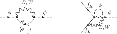
Refer to caption
Figure 7: Example of diagrams at 2-loop giving rise to λ​g12\lambda g_{1}^{2},λ​g22\lambda g_{2}^{2} terms in d16d_{16}.

There cannot exist any term proportional to λ​g32\lambda g_{3}^{2} or λ2\lambda^{2} in this case.

Having written the most general form of second order contributions to Y˙e\dot{Y}_{e}, we consider the fact that Tr⁡[Yi†​Yi]{\rm{Tr}}[Y_{i}^{\dagger}Y_{i}] (i∈{e,ν,U,D}i\in\{e,\nu,U,D\}) can only come from a complete fermionic loop in the Higgs self-energy correction, as already stated in Section III.1 and shown in Fig. 1. Hence, we can write the ratios as

d5:d6:d12U:d12D=1:r:3:3,\displaystyle d_{5}:d_{6}:d_{12}^{U}:d_{12}^{D}=1:r:3:3\;,
d7:d8:d13U:d13D=1:r:3:3,\displaystyle d_{7}:d_{8}:d_{13}^{U}:d_{13}^{D}=1:r:3:3\;, (131)

where rr for Type-I and Type-III seesaw is defined in Eq. (57) for SM and in Eq. (68) for MSSM. Hence, we can write

d5​Tr​[Ye†​Ye]+d6​Tr​[Yν†​Yν]+d12U​Tr​[YU†​YU]+d12D​Tr​[YD†​YD]→d12T​T,\displaystyle d_{5}{\rm{Tr}}[Y_{e}^{\dagger}Y_{e}]+d_{6}{\rm{Tr}}[Y_{\nu}^{\dagger}Y_{\nu}]+d_{12}^{U}{\rm{Tr}}[Y_{U}^{\dagger}Y_{U}]+d_{12}^{D}{\rm{Tr}}[Y_{D}^{\dagger}Y_{D}]\to d_{12}^{T}T\;,
d7​Tr​[Ye†​Ye]+d8​Tr​[Yν†​Yν]+d13U​Tr​[YU†​YU]+d13D​Tr​[YD†​YD]→d13T​T,\displaystyle d_{7}{\rm{Tr}}[Y_{e}^{\dagger}Y_{e}]+d_{8}{\rm{Tr}}[Y_{\nu}^{\dagger}Y_{\nu}]+d_{13}^{U}{\rm{Tr}}[Y_{U}^{\dagger}Y_{U}]+d_{13}^{D}{\rm{Tr}}[Y_{D}^{\dagger}Y_{D}]\to d_{13}^{T}T\;,

where TT is defined in Eq. (26) and d13Td_{13}^{T}, d14Td_{14}^{T} are expected to be of 𝒪⁡(1){\cal O}(1). Thus the most general form of Y˙e\dot{Y}_{e} becomes

(4​π)2​Y˙e|2-loop\displaystyle\left.(4\pi)^{2}\,\dot{Y}_{e}\right\arrowvert_{\text{2-loop}} =\displaystyle= Ye​(d1​Ye†​Ye​Ye†​Ye+d2​Ye†​Ye​Yν†​Yν+d3​Yν†​Yν​Ye†​Ye+d4​Yν†​Yν​Yν†​Yν)\displaystyle Y_{e}\left(d_{1}Y_{e}^{\dagger}Y_{e}Y_{e}^{\dagger}Y_{e}+d_{2}Y_{e}^{\dagger}Y_{e}Y_{\nu}^{\dagger}Y_{\nu}+d_{3}Y_{\nu}^{\dagger}Y_{\nu}Y_{e}^{\dagger}Y_{e}+d_{4}Y_{\nu}^{\dagger}Y_{\nu}Y_{\nu}^{\dagger}Y_{\nu}\right) (132)
+\displaystyle+ Ye​(d9​Tr​[Ye†​Ye​Ye†​Ye]+d10​Tr​[Yν†​Yν​Yν†​Yν]+d11​Tr​[Ye†​Ye​Yν†​Yν])\displaystyle Y_{e}\left(d_{9}{\rm{Tr}}[Y_{e}^{\dagger}Y_{e}Y_{e}^{\dagger}Y_{e}]+d_{10}{\rm{Tr}}[Y_{\nu}^{\dagger}Y_{\nu}Y_{\nu}^{\dagger}Y_{\nu}]+d_{11}{\rm{Tr}}[Y_{e}^{\dagger}Y_{e}Y_{\nu}^{\dagger}Y_{\nu}]\right)
+\displaystyle+ Ye​(d12g1​g12+d12g2​g22+d12λ​λ+d12T​T)​Ye†​Ye+Ye​(d13g1​g12+d14g2​g22+d13λ​λ+d13T​T)​Yν†​Yν\displaystyle Y_{e}\left(d_{12}^{g_{1}}g_{1}^{2}+d_{12}^{g_{2}}g_{2}^{2}+d_{12}^{\lambda}\lambda+d_{12}^{T}T\right)Y_{e}^{\dagger}Y_{e}+Y_{e}\left(d_{13}^{g_{1}}g_{1}^{2}+d_{14}^{g_{2}}g_{2}^{2}+d_{13}^{\lambda}\lambda+d_{13}^{T}T\right)Y_{\nu}^{\dagger}Y_{\nu}
+\displaystyle+ Ye​(d14​Tr​[Ye†​Ye]+d15​Tr​[Yν†​Yν])+d16​Ye.\displaystyle Y_{e}\left(d_{14}{\rm{Tr}}[Y_{e}^{\dagger}Y_{e}]+d_{15}{\rm{Tr}}[Y_{\nu}^{\dagger}Y_{\nu}]\right)+d_{16}Y_{e}\;.

B.2 2-loop running of YνY_{\nu}

Let us now consider the second order terms arising in the RGE of YνY_{\nu}. Considering Table 1, the transformation rules in Eqs. (15, 113), and the transformation properties in Eq. (114), we get that

Yν​Te​Te\displaystyle Y_{\nu}T_{e}T_{e} =\displaystyle= (3¯,1,3)⊗(8,1,1)⊗(8,1,1)∋(3¯,1,3),\displaystyle(\bar{3},1,3)\otimes(8,1,1)\otimes(8,1,1)\ni(\bar{3},1,3)\;, (133)
Yν​Te​Tν\displaystyle Y_{\nu}T_{e}T_{\nu} =\displaystyle= (3¯,1,3)⊗(8,1,1)⊗(8,1,1)∋(3¯,1,3),\displaystyle(\bar{3},1,3)\otimes(8,1,1)\otimes(8,1,1)\ni(\bar{3},1,3)\;, (134)
Yν​Tν​Te\displaystyle Y_{\nu}T_{\nu}T_{e} =\displaystyle= (3¯,1,3)⊗(8,1,1)⊗(8,1,1)∋(3¯,1,3),\displaystyle(\bar{3},1,3)\otimes(8,1,1)\otimes(8,1,1)\ni(\bar{3},1,3)\;, (135)
Yν​Tν​Tν\displaystyle Y_{\nu}T_{\nu}T_{\nu} =\displaystyle= (3¯,1,3)⊗(8,1,1)⊗(8,1,1)∋(3¯,1,3),\displaystyle(\bar{3},1,3)\otimes(8,1,1)\otimes(8,1,1)\ni(\bar{3},1,3)\;, (136)
Yν​Tr​[Ye†​Ye]​Te\displaystyle Y_{\nu}{\rm{Tr}}[Y_{e}^{\dagger}Y_{e}]T_{e} =\displaystyle= (3¯,1,3)⊗(1,1,1)⊗(8,1,1)∋(3¯,1,3),\displaystyle(\bar{3},1,3)\otimes(1,1,1)\otimes(8,1,1)\ni(\bar{3},1,3)\;, (137)
Yν​Tr​[Yν†​Yν]​Te\displaystyle Y_{\nu}{\rm{Tr}}[Y_{\nu}^{\dagger}Y_{\nu}]T_{e} =\displaystyle= (3¯,1,3)⊗(1,1,1)⊗(8,1,1)∋(3¯,1,3),\displaystyle(\bar{3},1,3)\otimes(1,1,1)\otimes(8,1,1)\ni(\bar{3},1,3)\;, (138)
Yν​Tr​[Ye†​Ye]​Tν\displaystyle Y_{\nu}{\rm{Tr}}[Y_{e}^{\dagger}Y_{e}]T_{\nu} =\displaystyle= (3¯,1,3)⊗(1,1,1)⊗(8,1,1)∋(3¯,1,3),\displaystyle(\bar{3},1,3)\otimes(1,1,1)\otimes(8,1,1)\ni(\bar{3},1,3)\;, (139)
Yν​Tr​[Yν†​Yν]​Tν\displaystyle Y_{\nu}{\rm{Tr}}[Y_{\nu}^{\dagger}Y_{\nu}]T_{\nu} =\displaystyle= (3¯,1,3)⊗(1,1,1)⊗(8,1,1)∋(3¯,1,3),\displaystyle(\bar{3},1,3)\otimes(1,1,1)\otimes(8,1,1)\ni(\bar{3},1,3)\;, (140)
Yν​Tr​[Ye†​Ye​Ye†​Ye]\displaystyle Y_{\nu}{\rm{Tr}}[Y_{e}^{\dagger}Y_{e}Y_{e}^{\dagger}Y_{e}] =\displaystyle= (3¯,1,3)⊗(1,1,1)=(3¯,1,3),\displaystyle(\bar{3},1,3)\otimes(1,1,1)=(\bar{3},1,3)\;, (141)
Yν​Tr​[Yν†​Yν​Yν†​Yν]\displaystyle Y_{\nu}{\rm{Tr}}[Y_{\nu}^{\dagger}Y_{\nu}Y_{\nu}^{\dagger}Y_{\nu}] =\displaystyle= (3¯,1,3)⊗(1,1,1)=(3¯,1,3),\displaystyle(\bar{3},1,3)\otimes(1,1,1)=(\bar{3},1,3)\;, (142)
andYν​Tr​[Ye†​Ye​Yν†​Yν]\displaystyle{\rm and}\quad Y_{\nu}{\rm{Tr}}[Y_{e}^{\dagger}Y_{e}Y_{\nu}^{\dagger}Y_{\nu}] =\displaystyle= (3¯,1,3)⊗(1,1,1)=(3¯,1,3)\displaystyle(\bar{3},1,3)\otimes(1,1,1)=(\bar{3},1,3)\; (143)

are the only allowed combinations of five spurion fields that can appear on the RHS of Y˙ν\dot{Y}_{\nu} at second order. Hence, similar to Y˙e\dot{Y}_{e}, we can write the most general form of the second order contributions to Y˙ν\dot{Y}_{\nu} as

(4​π)2​Y˙ν|2-loop\displaystyle\left.(4\pi)^{2}\;\dot{Y}_{\nu}\right\arrowvert_{\text{2-loop}} ∼\displaystyle\sim Yν​(f~1​Te​Te+f~2​Te​Tν+f~3​Tν​Te+f~4​Tν​Tν)\displaystyle Y_{\nu}\left(\widetilde{f}_{1}T_{e}T_{e}+\widetilde{f}_{2}T_{e}T_{\nu}+\widetilde{f}_{3}T_{\nu}T_{e}+\widetilde{f}_{4}T_{\nu}T_{\nu}\right) (144)
+\displaystyle+ Yν​(f~5​Tr​[Ye†​Ye]​Te+f~6​Tr​[Yν†​Yν]​Te+f~7​Tr​[Ye†​Ye]​Tν+f~8​Tr​[Yν†​Yν]​Tν)\displaystyle Y_{\nu}\left(\widetilde{f}_{5}{\rm{Tr}}[Y_{e}^{\dagger}Y_{e}]T_{e}+\widetilde{f}_{6}{\rm{Tr}}[Y_{\nu}^{\dagger}Y_{\nu}]T_{e}+\widetilde{f}_{7}{\rm{Tr}}[Y_{e}^{\dagger}Y_{e}]T_{\nu}+\widetilde{f}_{8}{\rm{Tr}}[Y_{\nu}^{\dagger}Y_{\nu}]T_{\nu}\right)
+\displaystyle+ Yν​(f~9​Tr​[Ye†​Ye​Ye†​Ye]+f~10​Tr​[Yν†​Yν​Yν†​Yν]+f~11​Tr​[Ye†​Ye​Yν†​Yν])\displaystyle Y_{\nu}\left(\widetilde{f}_{9}{\rm{Tr}}[Y_{e}^{\dagger}Y_{e}Y_{e}^{\dagger}Y_{e}]+\widetilde{f}_{10}{\rm{Tr}}[Y_{\nu}^{\dagger}Y_{\nu}Y_{\nu}^{\dagger}Y_{\nu}]+\widetilde{f}_{11}{\rm{Tr}}[Y_{e}^{\dagger}Y_{e}Y_{\nu}^{\dagger}Y_{\nu}]\right)
+\displaystyle+ Yν​(f~12​Te+f~13​Tν+f~14​Tr​[Ye†​Ye]+f~15​Tr​[Yν†​Yν])+f~16​Ye.\displaystyle Y_{\nu}\left(\widetilde{f}_{12}T_{e}+\widetilde{f}_{13}T_{\nu}+\widetilde{f}_{14}{\rm{Tr}}[Y_{e}^{\dagger}Y_{e}]+\widetilde{f}_{15}{\rm{Tr}}[Y_{\nu}^{\dagger}Y_{\nu}]\right)+\widetilde{f}_{16}Y_{e}\;.

The above equation can be written in a simple form using the definitions of TeT_{e}, TνT_{\nu} from Table 1 and the ratio of the coefficient of the traces, as done in case of Y˙e\dot{Y}_{e}, to give

(4​π)2​Y˙ν|2-loop\displaystyle\left.(4\pi)^{2}\;\dot{Y}_{\nu}\right\arrowvert_{\text{2-loop}} =\displaystyle= Yν​(f1​Ye†​Ye​Ye†​Ye+f2​Ye†​Ye​Yν†​Yν+f3​Yν†​Yν​Ye†​Ye+f4​Yν†​Yν​Yν†​Yν)\displaystyle Y_{\nu}\left(f_{1}Y_{e}^{\dagger}Y_{e}Y_{e}^{\dagger}Y_{e}+f_{2}Y_{e}^{\dagger}Y_{e}Y_{\nu}^{\dagger}Y_{\nu}+f_{3}Y_{\nu}^{\dagger}Y_{\nu}Y_{e}^{\dagger}Y_{e}+f_{4}Y_{\nu}^{\dagger}Y_{\nu}Y_{\nu}^{\dagger}Y_{\nu}\right) (145)
+\displaystyle+ Yν​(f9​Tr​[Ye†​Ye​Ye†​Ye]+f10​Tr​[Yν†​Yν​Yν†​Yν]+f11​Tr​[Ye†​Ye​Yν†​Yν])\displaystyle Y_{\nu}\left(f_{9}{\rm{Tr}}[Y_{e}^{\dagger}Y_{e}Y_{e}^{\dagger}Y_{e}]+f_{10}{\rm{Tr}}[Y_{\nu}^{\dagger}Y_{\nu}Y_{\nu}^{\dagger}Y_{\nu}]+f_{11}{\rm{Tr}}[Y_{e}^{\dagger}Y_{e}Y_{\nu}^{\dagger}Y_{\nu}]\right)
+\displaystyle+ Yν​(f12g1​g12+f13g2​g22+f12λ​λ+f12T​T)​Ye†​Ye+Yν​(f13g1​g12+f13g2​g22+f13λ​λ+f13T​T)​Yν†​Yν\displaystyle Y_{\nu}\left(f_{12}^{g_{1}}g_{1}^{2}+f_{13}^{g_{2}}g_{2}^{2}+f_{12}^{\lambda}\lambda+f_{12}^{T}T\right)Y_{e}^{\dagger}Y_{e}+Y_{\nu}\left(f_{13}^{g_{1}}g_{1}^{2}+f_{13}^{g_{2}}g_{2}^{2}+f_{13}^{\lambda}\lambda+f_{13}^{T}T\right)Y_{\nu}^{\dagger}Y_{\nu}
+\displaystyle+ Yν​(f14​Tr​[Ye†​Ye]+f15​Tr​[Yν†​Yν])+f16​Yν,\displaystyle Y_{\nu}\left(f_{14}{\rm{Tr}}[Y_{e}^{\dagger}Y_{e}]+f_{15}{\rm{Tr}}[Y_{\nu}^{\dagger}Y_{\nu}]\right)+f_{16}Y_{\nu}\;,

with TT defined in Eq. (26). Here, f1,⋯,4f_{1,\cdots,4}, f9,⋯,11f_{9,\cdots,11}, f12xf_{12}^{x} and f13xf_{13}^{x} are expected to be 𝒪⁡(1){\cal O}(1) numbers. fif_{i} (ii=14,15,16) will have similar forms as did_{i} (ii=14,15,16), as given in Eqs. (129) and (130) respectively, with all fixf_{i}^{x} (ii=14,15,16) being 𝒪⁡(1){\cal O}(1) quantities. As before, we have not written the terms of the form Tr⁡[Yi†​Yi]⋅Tr⁡[Yj†​Yj]{\rm{Tr}}[Y_{i}^{\dagger}Y_{i}]\cdot{\rm{Tr}}[Y_{j}^{\dagger}Y_{j}], i,j∈{e,ν,U,D}i,j\in\{e,\nu,U,D\}, since such terms cannot be generated at 2-loop.

B.3 2-loop running of MνM_{\nu}

Next, we discuss the second order contribution to M˙ν\dot{M}_{\nu}. Using Table 1 and the SU⁡(3){\rm{SU}}(3) algebra given in Eqs. (35) and (113), we obtain that

Mν​Tν′​Tν′\displaystyle M_{\nu}T_{\nu}^{\prime}T_{\nu}^{\prime} =\displaystyle= (1,1,6)⊗(1,1,8)⊗(1,1,8)∋(1,1,6),\displaystyle(1,1,6)\otimes(1,1,8)\otimes(1,1,8)\ni(1,1,6)\;, (146)
Mν​(Yν​Ye†​Ye​Yν†)\displaystyle M_{\nu}\left(Y_{\nu}Y_{e}^{\dagger}Y_{e}Y_{\nu}^{\dagger}\right) =\displaystyle= (1,1,6)⊗(3¯,1,3)⊗(8⊕1,1,1)⊗(3,1,3¯)∋(1,1,6),\displaystyle(1,1,6)\otimes(\bar{3},1,3)\otimes(8\oplus 1,1,1)\otimes(3,1,\bar{3})\ni(1,1,6)\;, (147)
Tν′T​Mν​Tν′\displaystyle T_{\nu}^{\prime T}M_{\nu}T_{\nu}^{\prime} =\displaystyle= (1,1,8)⊗(1,1,6)⊗(1,1,8)∋(1,1,6),\displaystyle(1,1,8)\otimes(1,1,6)\otimes(1,1,8)\ni(1,1,6)\;, (148)
Mν​Tr​[Ye†​Ye]​Tν′\displaystyle M_{\nu}{\rm{Tr}}[Y_{e}^{\dagger}Y_{e}]T_{\nu}^{\prime} =\displaystyle= (1,1,6)⊗(1,1,1)⊗(1,1,8)∋(1,1,6),\displaystyle(1,1,6)\otimes(1,1,1)\otimes(1,1,8)\ni(1,1,6)\;, (149)
andMν​Tr​[Yν†​Yν]​Tν′\displaystyle{\rm and}\quad M_{\nu}{\rm{Tr}}[Y_{\nu}^{\dagger}Y_{\nu}]T_{\nu}^{\prime} =\displaystyle= (1,1,6)⊗(1,1,1)⊗(1,1,8)∋(1,1,6)\displaystyle(1,1,6)\otimes(1,1,1)\otimes(1,1,8)\ni(1,1,6) (150)

are the only combinations of five spurion fields that can contribute to M˙ν\dot{M}_{\nu}. The term in Eq. (147), not present in Table 1, is an allowed combination at second order. Here we have considered the fact that MνM_{\nu} couples only to the right-handed neutrinos and hence M˙ν\dot{M}_{\nu} cannot contain trace of four spurions at second order. Apart from the above terms, there will also be terms with three spurions and two other couplings in the theory, transforming trivially under GLF{\rm G}_{\rm{LF}}. Terms containing one spurion and four other couplings are also allowed at this order. However, MνM_{\nu} being coupled to right-handed neutrinos alone, M˙ν\dot{M}_{\nu} will not contain terms proportional to trace of four YU,DY_{U,D} and also no g14g_{1}^{4} or λ2\lambda^{2}. If the right-handed neutrinos are singlets under the gauge group, as is the case for Type-I seesaw, they will not have any SU​(2)L{\rm{SU}}(2)_{L} or SU​(3)C{\rm{SU}}(3)_{C} charges and hence terms proportional to g24g_{2}^{4}, g34g_{3}^{4} be absent. However, for Type-III seesaw scenario these are triplet under SU​(2)L{\rm{SU}}(2)_{L} and hence g24g_{2}^{4} contribution is expected to be there.

Finally, symmetrizing over the O(3)νR{}_{\nu_{R}} indices, the most general form of the 2-loop contribution to M˙ν\dot{M}_{\nu} can be written as

(4​π)2​M˙ν|2-loop\displaystyle\left.(4\pi)^{2}\;\dot{M}_{\nu}\right\arrowvert_{\text{2-loop}} =\displaystyle= h~12​(Mν​(Tν′​Tν′)+(Tν′​Tν′)T​Mν)+h22​(Mν​(Yν​Ye†​Ye​Yν†)+(Yν​Ye†​Ye​Yν†)T​Mν)\displaystyle\frac{\widetilde{h}_{1}}{2}\left(M_{\nu}\left(T_{\nu}^{\prime}T_{\nu}^{\prime}\right)+\left(T_{\nu}^{\prime}T_{\nu}^{\prime}\right)^{T}M_{\nu}\right)+\frac{h_{2}}{2}\left(M_{\nu}\left(Y_{\nu}Y_{e}^{\dagger}Y_{e}Y_{\nu}^{\dagger}\right)+\left(Y_{\nu}Y_{e}^{\dagger}Y_{e}Y_{\nu}^{\dagger}\right)^{T}M_{\nu}\right) (151)
+\displaystyle+ h~3​Tν′T​Mν​Tν′+12​(h~4′​Tr​[Ye†​Ye]+h~4′′​Tr​[Yν†​Yν])​(Mν​Tν′+Tν′T​Mν)\displaystyle\widetilde{h}_{3}T_{\nu}^{\prime T}M_{\nu}T_{\nu}^{\prime}+\frac{1}{2}\left(\widetilde{h}_{4}^{\prime}{\rm{Tr}}[Y_{e}^{\dagger}Y_{e}]+\widetilde{h}_{4}^{\prime\prime}{\rm{Tr}}[Y_{\nu}^{\dagger}Y_{\nu}]\right)\left(M_{\nu}T_{\nu}^{\prime}+T_{\nu}^{\prime T}M_{\nu}\right)
+\displaystyle+ h~42​(Mν​Tν′+Tν′T​Mν)+h~5​g24​Mν.\displaystyle\frac{\widetilde{h}_{4}}{2}\left(M_{\nu}T_{\nu}^{\prime}+T_{\nu}^{\prime T}M_{\nu}\right)+\widetilde{h}_{5}g_{2}^{4}M_{\nu}\;.

Eq. (151) can be simplified using the definition of Tν′T_{\nu}^{\prime} and the fact that terms proportional to Tr⁡[Yi†​Yi]​(i∈{e,ν,U,D}){\rm{Tr}}[Y_{i}^{\dagger}Y_{i}]~(i\in\{e,\nu,U,D\}) appear only in the combination TT, defined in Eq. (26), to get

(4​π)2​M˙ν|2-loop\displaystyle\left.(4\pi)^{2}\;\dot{M}_{\nu}\right\arrowvert_{\text{2-loop}} =\displaystyle= h1​(Mν​(Yν​Yν†​Yν​Yν†)+(Yν​Yν†​Yν​Yν†)T​Mν)\displaystyle h_{1}\left(M_{\nu}\left(Y_{\nu}Y_{\nu}^{\dagger}Y_{\nu}Y_{\nu}^{\dagger}\right)+\left(Y_{\nu}Y_{\nu}^{\dagger}Y_{\nu}Y_{\nu}^{\dagger}\right)^{T}M_{\nu}\right) (152)
+\displaystyle+ h2​(Mν​(Yν​Ye†​Ye​Yν†)+(Yν​Ye†​Ye​Yν†)T​Mν)+h3​(Yν​Yν†)T​Mν​(Yν​Yν†)\displaystyle h_{2}\left(M_{\nu}\left(Y_{\nu}Y_{e}^{\dagger}Y_{e}Y_{\nu}^{\dagger}\right)+\left(Y_{\nu}Y_{e}^{\dagger}Y_{e}Y_{\nu}^{\dagger}\right)^{T}M_{\nu}\right)+h_{3}\left(Y_{\nu}Y_{\nu}^{\dagger}\right)^{T}M_{\nu}\left(Y_{\nu}Y_{\nu}^{\dagger}\right)
+\displaystyle+ h4​(Mν​(Yν​Yν†)+(Yν​Yν†)T​Mν)+h5​g24​Mν,\displaystyle h_{4}\left(M_{\nu}\left(Y_{\nu}Y_{\nu}^{\dagger}\right)+\left(Y_{\nu}Y_{\nu}^{\dagger}\right)^{T}M_{\nu}\right)+h_{5}g_{2}^{4}M_{\nu}\;,

where h1h_{1}, h2h_{2}, h3h_{3} and h5h_{5} are expected to be 𝒪⁡(1){\cal O}(1) numbers in general. For Type-I seesaw, h5=0h_{5}=0. In writing Eq. (152), we have considered the fact that terms with Tr⁡[Yi†​Yi]⋅Tr⁡[Yj†​Yj]​(i,j∈{e,ν}){\rm{Tr}}[Y_{i}^{\dagger}Y_{i}]\cdot{\rm{Tr}}[Y_{j}^{\dagger}Y_{j}](i,j\in\{e,\nu\}) cannot be present at 2-loop. h4h_{4} can in general be a linear function of g12g_{1}^{2}, g22g_{2}^{2}, λ\lambda and TT and be given by

h4=h4g1​g12+h4g2​g22+h4λ​λ+h4T​T,h_{4}=h_{4}^{g_{1}}g_{1}^{2}+h_{4}^{g_{2}}g_{2}^{2}+h_{4}^{\lambda}\lambda+h_{4}^{T}T\;, (153)

where all h4xh_{4}^{x} must be of 𝒪⁡(1){\cal O}(1). In writing Eq. (152) we have used the symmetry property of MνM_{\nu}: MνT=MνM_{\nu}^{T}=M_{\nu}. Leptons and Higgs, being singlets under SU​(3)C{\rm{SU}}(3)_{C}, h4h_{4} will not involve g32g_{3}^{2}.

As before, we expect Eq. (152) to give the right-handed projection of M˙ν\dot{M}_{\nu} only. The most general form of M˙ν\dot{M}_{\nu} will be given by

(4​π)2​M˙ν|2-loop\displaystyle(4\pi)^{2}\left.\dot{M}_{\nu}\right\arrowvert_{\text{\tiny{2-loop}}} =\displaystyle= h1​[(Mν​(Yν​Yν†​Yν​Yν†)+(Yν​Yν†​Yν​Yν†)T​Mν)​PR+(Mν​(Yν​Yν†​Yν​Yν†)T+(Yν​Yν†​Yν​Yν†)​Mν)​PL]\displaystyle h_{1}\left[\left(M_{\nu}\left(Y_{\nu}Y_{\nu}^{\dagger}Y_{\nu}Y_{\nu}^{\dagger}\right)+\left(Y_{\nu}Y_{\nu}^{\dagger}Y_{\nu}Y_{\nu}^{\dagger}\right)^{T}M_{\nu}\right)P_{R}+\left(M_{\nu}\left(Y_{\nu}Y_{\nu}^{\dagger}Y_{\nu}Y_{\nu}^{\dagger}\right)^{T}+\left(Y_{\nu}Y_{\nu}^{\dagger}Y_{\nu}Y_{\nu}^{\dagger}\right)M_{\nu}\right)P_{L}\right] (154)
+\displaystyle+ h2​[(Mν​(Yν​Ye†​Ye​Yν†)+(Yν​Ye†​Ye​Yν†)T​Mν)​PR+(Mν​(Yν​Ye†​Ye​Yν†)T+(Yν​Ye†​Ye​Yν†)​Mν)​PL]\displaystyle h_{2}\left[\left(M_{\nu}\left(Y_{\nu}Y_{e}^{\dagger}Y_{e}Y_{\nu}^{\dagger}\right)+\left(Y_{\nu}Y_{e}^{\dagger}Y_{e}Y_{\nu}^{\dagger}\right)^{T}M_{\nu}\right)P_{R}+\left(M_{\nu}\left(Y_{\nu}Y_{e}^{\dagger}Y_{e}Y_{\nu}^{\dagger}\right)^{T}+\left(Y_{\nu}Y_{e}^{\dagger}Y_{e}Y_{\nu}^{\dagger}\right)M_{\nu}\right)P_{L}\right]
+\displaystyle+ h3​[(Yν​Yν†)T​Mν​(Yν​Yν†)​PR+(Yν​Yν†)​Mν​(Yν​Yν†)T​PL]\displaystyle h_{3}\left[\left(Y_{\nu}Y_{\nu}^{\dagger}\right)^{T}M_{\nu}\left(Y_{\nu}Y_{\nu}^{\dagger}\right)P_{R}+\left(Y_{\nu}Y_{\nu}^{\dagger}\right)M_{\nu}\left(Y_{\nu}Y_{\nu}^{\dagger}\right)^{T}P_{L}\right]
+\displaystyle+ h4​[(Mν​(Yν​Yν†)+(Yν​Yν†)T​Mν)​PR+(Mν​(Yν​Yν†)T+(Yν​Yν†)​Mν)​PL]+h5​g24​Mν.\displaystyle h_{4}\left[\left(M_{\nu}\left(Y_{\nu}Y_{\nu}^{\dagger}\right)+\left(Y_{\nu}Y_{\nu}^{\dagger}\right)^{T}M_{\nu}\right)P_{R}+\left(M_{\nu}\left(Y_{\nu}Y_{\nu}^{\dagger}\right)^{T}+\left(Y_{\nu}Y_{\nu}^{\dagger}\right)M_{\nu}\right)P_{L}\right]+h_{5}g_{2}^{4}M_{\nu}\;.

B.4 2-loop running of the left-handed mass mνm_{\nu} at μ<MR\mu<M_{R}

At the energy scale μ<MR\mu<M_{R}, the flavor symmetry group is GLF′{\rm G}_{\rm{LF}}^{\prime} and Ye​(3¯,3)Y_{e}(\bar{3},3), mν​(6,1)m_{\nu}(6,1) are the only spurions in the theory. Let us first consider the running of YeY_{e} at this scale which can be obtained from Eq. (132) simply by setting the coefficients of terms containing YνY_{\nu} to zero and we have

(4​π)2​Y˙e|2-loop\displaystyle\left.(4\pi)^{2}\;\dot{Y}_{e}\right\arrowvert_{\text{2-loop}} =\displaystyle= Ye​(d1​Ye†​Ye​Ye†​Ye+d9​Tr​[Ye†​Ye​Ye†​Ye]+(d12g1​g12+d12g2​g22+d12λ​λ+d12T​T)​Ye†​Ye)\displaystyle Y_{e}\left(d_{1}Y_{e}^{\dagger}Y_{e}Y_{e}^{\dagger}Y_{e}+d_{9}{\rm{Tr}}[Y_{e}^{\dagger}Y_{e}Y_{e}^{\dagger}Y_{e}]+\left(d_{12}^{g_{1}}g_{1}^{2}+d_{12}^{g_{2}}g_{2}^{2}+d_{12}^{\lambda}\lambda+d_{12}^{T}T\right)Y_{e}^{\dagger}Y_{e}\right) (155)
+\displaystyle+ Ye​(d14g1​g12+d14g2​g22)​Tr​[Ye†​Ye]+d16​Ye,\displaystyle Y_{e}\left(d^{g_{1}}_{14}g_{1}^{2}+d^{g_{2}}_{14}g_{2}^{2}\right){\rm{Tr}}[Y_{e}^{\dagger}Y_{e}]+d_{16}Y_{e}\;,

where d16d_{16} is given by Eq. (130). d1d_{1}, d9d_{9}, d12xd_{12}^{x} and d14xd_{14}^{x} are expected to be 𝒪⁡(1){\cal O}(1) numbers.

Now we consider the running of the left-handed mass mνm_{\nu}. Using Table 1, the transformation rules in Eq. (114) and the SU⁡(3){\rm{SU}}(3) algebra given in Eqs. (35, 113) we get the second order contributions to m˙ν\dot{m}_{\nu} to contain the following combinations of five spurions:

mν​Te​Te\displaystyle m_{\nu}T_{e}T_{e} =\displaystyle= (6,1)⊗(8,1)⊗(8,1)∋(6,1),\displaystyle(6,1)\otimes(8,1)\otimes(8,1)\ni(6,1)\;, (156)
TeT​mν​Te\displaystyle T_{e}^{T}m_{\nu}T_{e} =\displaystyle= (8,1)⊗(6,1)⊗(8,1)∋(6,1),\displaystyle(8,1)\otimes(6,1)\otimes(8,1)\ni(6,1)\;, (157)
mν​Tr​[Ye†​Ye]​Te\displaystyle m_{\nu}{\rm{Tr}}[Y_{e}^{\dagger}Y_{e}]T_{e} =\displaystyle= (6,1)⊗(1,1)⊗(8,1)∋(6,1),\displaystyle(6,1)\otimes(1,1)\otimes(8,1)\ni(6,1)\;, (158)
andmν​Tr​[Ye†​Ye​Ye†​Ye]\displaystyle{\rm and}\quad m_{\nu}{\rm{Tr}}[Y_{e}^{\dagger}Y_{e}Y_{e}^{\dagger}Y_{e}] =\displaystyle= (6,1)⊗(1,1)=(6,1),\displaystyle(6,1)\otimes(1,1)=(6,1)\;, (159)

where the terms proportional to Tr⁡[Ye†​Ye]⋅Tr⁡[Ye†​Ye]{\rm{Tr}}[Y_{e}^{\dagger}Y_{e}]\cdot{\rm{Tr}}[Y_{e}^{\dagger}Y_{e}] are to be removed since such terms cannot arise at 2-loop. Finally, symmetrizing over the SU​(3)lL{\rm{SU}}(3)_{l_{L}} indices, we write down the most general form of m˙ν\dot{m}_{\nu} at second order as

(4​π)2​m˙ν|2-loop\displaystyle\left.(4\pi)^{2}\;\dot{m}_{\nu}\right\arrowvert_{\text{2-loop}} =\displaystyle= r1​(mν​(Ye†​Ye​Ye†​Ye)+(Ye†​Ye​Ye†​Ye)T​mν)+r2​(Ye†​Ye)T​mν​(Ye†​Ye)\displaystyle r_{1}\left(m_{\nu}\left(Y_{e}^{\dagger}Y_{e}Y_{e}^{\dagger}Y_{e}\right)+\left(Y_{e}^{\dagger}Y_{e}Y_{e}^{\dagger}Y_{e}\right)^{T}m_{\nu}\right)+r_{2}\left(Y_{e}^{\dagger}Y_{e}\right)^{T}m_{\nu}\left(Y_{e}^{\dagger}Y_{e}\right) (160)
+\displaystyle+ r3​Tr​[Ye†​Ye]​(mν​(Ye†​Ye)+(Ye†​Ye)T​mν)+r4​Tr​[Ye†​Ye​Ye†​Ye]​mν\displaystyle r_{3}{\rm{Tr}}[Y_{e}^{\dagger}Y_{e}]\left(m_{\nu}\left(Y_{e}^{\dagger}Y_{e}\right)+\left(Y_{e}^{\dagger}Y_{e}\right)^{T}m_{\nu}\right)+r_{4}{\rm{Tr}}[Y_{e}^{\dagger}Y_{e}Y_{e}^{\dagger}Y_{e}]m_{\nu}
+\displaystyle+ r5​(mν​(Ye†​Ye)+(Ye†​Ye)T​mν)+r6​mν,\displaystyle r_{5}\left(m_{\nu}\left(Y_{e}^{\dagger}Y_{e}\right)+\left(Y_{e}^{\dagger}Y_{e}\right)^{T}m_{\nu}\right)+r_{6}m_{\nu}\;,

where r1,r2,r3,r4r_{1},r_{2},r_{3},r_{4} are expected to be of 𝒪⁡(1){\cal O}(1), while the general forms of r5,r6r_{5},r_{6} are

r5\displaystyle r_{5} =\displaystyle= r5U​Tr​[YU†​YU]+r5D​Tr​[YD†​YD]+r5g1​g12+r5g2​g22+r5λ​λ,\displaystyle r_{5}^{U}{\rm{Tr}}[Y_{U}^{\dagger}Y_{U}]+r_{5}^{D}{\rm{Tr}}[Y_{D}^{\dagger}Y_{D}]+r_{5}^{g_{1}}g_{1}^{2}+r_{5}^{g_{2}}g_{2}^{2}+r_{5}^{\lambda}\lambda\;, (161)
r6\displaystyle r_{6} =\displaystyle= r6U​U​Tr​[YU†​YU​YU†​YU]+r6D​D​Tr​[YD†​YD​YD†​YD]+r6U​D​Tr​[YU†​YU​YD†​YD]\displaystyle r_{6}^{UU}{\rm{Tr}}[Y_{U}^{\dagger}Y_{U}Y_{U}^{\dagger}Y_{U}]+r_{6}^{DD}{\rm{Tr}}[Y_{D}^{\dagger}Y_{D}Y_{D}^{\dagger}Y_{D}]+r_{6}^{UD}{\rm{Tr}}[Y_{U}^{\dagger}Y_{U}Y_{D}^{\dagger}Y_{D}] (162)
+\displaystyle+ (r6g1​U​g12+r6g2​U​g22+r6g3​U​g32)​Tr​[YU†​YU]+(r6g1​D​g12+r6g2​D​g22+r6g3​D​g32)​Tr​[YD†​YD]\displaystyle\left(r_{6}^{g_{1}U}g_{1}^{2}+r_{6}^{g_{2}U}g_{2}^{2}+r_{6}^{g_{3}U}g_{3}^{2}\right){\rm{Tr}}[Y_{U}^{\dagger}Y_{U}]+\left(r_{6}^{g_{1}D}g_{1}^{2}+r_{6}^{g_{2}D}g_{2}^{2}+r_{6}^{g_{3}D}g_{3}^{2}\right){\rm{Tr}}[Y_{D}^{\dagger}Y_{D}]
+\displaystyle+ (r6g1​λ​g12+r6g2​λ​g22)​λ+r6λ​λ2+r6g1​g14+r6g2​g24+r6g1​g2​g12​g22,\displaystyle\left(r_{6}^{g_{1}\lambda}g_{1}^{2}+r_{6}^{g_{2}\lambda}g_{2}^{2}\right)\lambda+r_{6}^{\lambda}\lambda^{2}+r_{6}^{g_{1}}g_{1}^{4}+r_{6}^{g_{2}}g_{2}^{4}+r_{6}^{g_{1}g_{2}}g_{1}^{2}g_{2}^{2}\;,

with all r5x,r6xr_{5}^{x},r_{6}^{x} being expected to be 𝒪⁡(1){\cal O}(1) numbers. We can further simplify by considering the fact that terms proportional to Tr⁡[Yi†​Yi]​(i∈{e,U,D}){\rm{Tr}}[Y_{i}^{\dagger}Y_{i}](i\in\{e,U,D\}) come through a complete fermion loop in Higgs self-energy corrections and hence we must have

r3​Tr​[Ye†​Ye]+r5U​Tr​[YU†​YU]+r5D​Tr​[YD†​YD]→r5T​T′,r_{3}{\rm{Tr}}[Y_{e}^{\dagger}Y_{e}]+r_{5}^{U}{\rm{Tr}}[Y_{U}^{\dagger}Y_{U}]+r_{5}^{D}{\rm{Tr}}[Y_{D}^{\dagger}Y_{D}]\to r_{5}^{T}\,T^{\prime}\;,

where T′T^{\prime} is defined in Eq. (50) and r5Tr_{5}^{T} is of 𝒪⁡(1){\cal O}(1). So the 2-loop contribution to m˙ν\dot{m}_{\nu} becomes

(4​π)2​m˙ν|2-loop\displaystyle\left.(4\pi)^{2}\;\dot{m}_{\nu}\right\arrowvert_{\text{2-loop}} =\displaystyle= r1​(mν​(Ye†​Ye​Ye†​Ye)+(Ye†​Ye​Ye†​Ye)T​mν)+r2​(Ye†​Ye)T​mν​(Ye†​Ye)\displaystyle r_{1}\left(m_{\nu}\left(Y_{e}^{\dagger}Y_{e}Y_{e}^{\dagger}Y_{e}\right)+\left(Y_{e}^{\dagger}Y_{e}Y_{e}^{\dagger}Y_{e}\right)^{T}m_{\nu}\right)+r_{2}\left(Y_{e}^{\dagger}Y_{e}\right)^{T}m_{\nu}\left(Y_{e}^{\dagger}Y_{e}\right) (163)
+\displaystyle+ r4​Tr​[Ye†​Ye​Ye†​Ye]​mν+r5′​(mν​(Ye†​Ye)+(Ye†​Ye)T​mν)+r6​mν,\displaystyle r_{4}{\rm{Tr}}[Y_{e}^{\dagger}Y_{e}Y_{e}^{\dagger}Y_{e}]m_{\nu}+r_{5}^{\prime}\left(m_{\nu}\left(Y_{e}^{\dagger}Y_{e}\right)+\left(Y_{e}^{\dagger}Y_{e}\right)^{T}m_{\nu}\right)+r_{6}m_{\nu}\;,

with

r5′\displaystyle r_{5}^{\prime} =\displaystyle= r5T​T′+r5g1​g12+r5g2​g22+r5λ​λ.\displaystyle r_{5}^{T}\,T^{\prime}+r_{5}^{g_{1}}g_{1}^{2}+r_{5}^{g_{2}}g_{2}^{2}+r_{5}^{\lambda}\lambda\;. (164)

B.5 Results

First, let us consider the case of the SM. Second order contributions to the RG evolution equations of YeY_{e}, YνY_{\nu}, MνM_{\nu} or mνm_{\nu} are not available in the literature for right-handed neutrino extended SM (Type-I or Type-III) in general. In Ref. [24], the contribution to m˙ν\dot{m}_{\nu} proportional to r2r_{2} in Eq. (163), for Type-I seesaw, is presented that gives

r2=2.r_{2}=2\;. (165)

Thus r2r_{2} is of 𝒪⁡(1){\cal O}(1), as expected. In the future, once a full calculation is done, it can be checked against our results.

Next, we move to the case of the MSSM. Unlike the case of SM, there are existing results for second order contributions in extended MSSM for Type-I seesaw [12], obtained from exact computations. In order to compare the results with the equations obtained above, we keep the following facts in mind:

  • •

    Higgs self-coupling λ\lambda is absent in MSSM, hence all terms proportional to λ\lambda will vanish.

  • •

    Terms with Ye†​YeY_{e}^{\dagger}Y_{e} can only contain Tr⁡[Ye†​Ye]{\rm{Tr}}[Y_{e}^{\dagger}Y_{e}] and Tr⁡[YD†​YD]{\rm{Tr}}[Y_{D}^{\dagger}Y_{D}], while terms with Yν†​YνY_{\nu}^{\dagger}Y_{\nu} can only contain Tr⁡[Yν†​Yν]{\rm{Tr}}[Y_{\nu}^{\dagger}Y_{\nu}] and Tr⁡[YU†​YU]{\rm{Tr}}[Y_{U}^{\dagger}Y_{U}]. Moreover they will appear only in the combinations TUT_{U} and TDT_{D}, defined in Eqs.(66) and (67) respectively. Thus, the terms present will be TD​Ye†​YeT_{D}Y_{e}^{\dagger}Y_{e} and TU​Yν†​YνT_{U}Y_{\nu}^{\dagger}Y_{\nu}.

  • •

    Y˙e\dot{Y}_{e} cannot have terms proportional to Tr⁡[Yν†​Yν​Yν†​Yν]{\rm{Tr}}[Y_{\nu}^{\dagger}Y_{\nu}Y_{\nu}^{\dagger}Y_{\nu}] or Tr⁡[YU†​YU​YU†​YU]{\rm{Tr}}[Y_{U}^{\dagger}Y_{U}Y_{U}^{\dagger}Y_{U}]. Similarly, Y˙ν\dot{Y}_{\nu} cannot have terms proportional to Tr⁡[Ye†​Ye​Ye†​Ye]{\rm{Tr}}[Y_{e}^{\dagger}Y_{e}Y_{e}^{\dagger}Y_{e}] and Tr⁡[YD†​YD​YD†​YD]{\rm{Tr}}[Y_{D}^{\dagger}Y_{D}Y_{D}^{\dagger}Y_{D}]. Hence

    d10\displaystyle d_{10} =\displaystyle= 0,d16U​U=0,f9=0,f16D​D=0.\displaystyle 0\;,\qquad d_{16}^{UU}=0\;,\qquad f_{9}=0\;,\qquad f_{16}^{DD}=0\;. (166)
  • •

    Since YeY_{e} couples to HDH_{D} only, Y˙e\dot{Y}_{e} cannot contain terms gi2​Tr​[Yν†​Yν]g_{i}^{2}{\rm{Tr}}[Y_{\nu}^{\dagger}Y_{\nu}] and gi2​Tr​[YU†​YU]g_{i}^{2}{\rm{Tr}}[Y_{U}^{\dagger}Y_{U}]. Similarly, Y˙ν\dot{Y}_{\nu} cannot have terms gi2​Tr​[Ye†​Ye]g_{i}^{2}{\rm{Tr}}[Y_{e}^{\dagger}Y_{e}] or gi2​Tr​[YD†​YD]g_{i}^{2}{\rm{Tr}}[Y_{D}^{\dagger}Y_{D}]. Thus,

    d15g1\displaystyle d_{15}^{g_{1}} =\displaystyle= d15g2=0,d16g1​U=d16g2​U=d16g3​U=0\displaystyle d_{15}^{g_{2}}=0\;,\qquad d_{16}^{g_{1}U}=d_{16}^{g_{2}U}=d_{16}^{g_{3}U}=0\;
    f14g1\displaystyle f_{14}^{g_{1}} =\displaystyle= f14g2=0,f16g1​D=f16g2​D=f16g3​D=0.\displaystyle f_{14}^{g_{2}}=0\;,\qquad f_{16}^{g_{1}D}=f_{16}^{g_{2}D}=f_{16}^{g_{3}D}=0\;. (167)
  • •

    The right-handed Majorana mass MνM_{\nu} couples only to the right-handed neutrinos which interacts with HUH_{U}, and not with HDH_{D}, and so h4h_{4} in Eq. (153) becomes

    h4=h4g1​g12+h4g2​g22+h4T​TU.h_{4}=h_{4}^{g_{1}}g_{1}^{2}+h_{4}^{g_{2}}g_{2}^{2}+h_{4}^{T}T_{U}\;. (168)
  • •

    Only HUH_{U} is involved in the definition of the effective left-handed Majorana mass mνm_{\nu}, and hence we must have

    T′=TU′=Tr⁡[Ye†​Ye]+3​Tr​[YU†​YU],T^{\prime}=T_{U}^{\prime}={\rm{Tr}}[Y_{e}^{\dagger}Y_{e}]+3{\rm{Tr}}[Y_{U}^{\dagger}Y_{U}]\;, (169)

    and r6r_{6} in Eq. (162) will have

    r6D​D=0,r6g1​D=0,r6g2​D=0,r6g3​D=0.\displaystyle r_{6}^{DD}=0\;,\qquad r_{6}^{g_{1}D}=0\;,\qquad r_{6}^{g_{2}D}=0\;,\qquad r_{6}^{g_{3}D}=0\;. (170)

Let us now compare the coefficients with the values obtained with exact computation [12]. For YeY_{e} evolution we get

d1\displaystyle d_{1} =\displaystyle= −4,d2=0,d3=−2,d4=−2,d9=−3,d11=−1,\displaystyle-4\;,\qquad d_{2}=0\;,\qquad d_{3}=-2\;,\qquad d_{4}=-2\;,\qquad d_{9}=-3\;,\qquad d_{11}=-1\;,
d12g1\displaystyle d_{12}^{g_{1}} =\displaystyle= 0,d12g2=6,d12T=−3,d13g1=0,d13g2=0,d13T=−1,\displaystyle 0\;,\qquad d_{12}^{g_{2}}=6\;,\qquad d_{12}^{T}=-3\;,\qquad d_{13}^{g_{1}}=0\;,\qquad d_{13}^{g_{2}}=0\;,\qquad d_{13}^{T}=-1\;,
d14g1\displaystyle d_{14}^{g_{1}} =\displaystyle= 65,d14g2=0,d16D​D=−9,d16U​D=−3,d16g1​D=−25,\displaystyle\frac{6}{5}\;,\qquad d_{14}^{g_{2}}=0\;,\qquad d_{16}^{DD}=-9\;,\qquad d_{16}^{UD}=-3\;,\qquad d_{16}^{g_{1}D}=-\frac{2}{5}\;,
d16g2​D\displaystyle d_{16}^{g_{2}D} =\displaystyle= 0,d16g3​D=16,d16g1=272,d16g2=152,d16g1​g2=95.\displaystyle 0\;,\qquad d_{16}^{g_{3}D}=16\;,\qquad d_{16}^{g_{1}}=\frac{27}{2}\;,\qquad d_{16}^{g_{2}}=\frac{15}{2}\;,\qquad d_{16}^{g_{1}g_{2}}=\frac{9}{5}\;. (171)

Comparing the coefficients of Y˙ν\dot{Y}_{\nu}, we get

f1\displaystyle f_{1} =\displaystyle= −2,f2=−2,f3=0,f4=−4,f10=−3,f11=−1,\displaystyle-2\;,\qquad f_{2}=-2\;,\qquad f_{3}=0\;,\qquad f_{4}=-4\;,\qquad f_{10}=-3\;,\qquad f_{11}=-1\;,
f12g1\displaystyle f_{12}^{g_{1}} =\displaystyle= 65,f12g2=0,f12T=−1,f13g1=65,f13g2=6,f13T=−3,\displaystyle\frac{6}{5}\;,\qquad f_{12}^{g_{2}}=0\;,\qquad f_{12}^{T}=-1\;,\qquad f_{13}^{g_{1}}=\frac{6}{5}\;,\qquad f_{13}^{g_{2}}=6\;,\qquad f_{13}^{T}=-3\;,
f15g1\displaystyle f_{15}^{g_{1}} =\displaystyle= 0,f15g2=0,f16U​U=−9,f16U​D=−3,f16g1​U=45,\displaystyle 0\;,\qquad f_{15}^{g_{2}}=0\;,\qquad f_{16}^{UU}=-9\;,\qquad f_{16}^{UD}=-3\;,\qquad f_{16}^{g_{1}U}=\frac{4}{5}\;,
f16g2​U\displaystyle f_{16}^{g_{2}U} =\displaystyle= 0,f16g3​U=16,f16g1=20750,f16g2=152,f16g1​g2=95.\displaystyle 0\;,\qquad f_{16}^{g_{3}U}=16\;,\qquad f_{16}^{g_{1}}=\frac{207}{50}\;,\qquad f_{16}^{g_{2}}=\frac{15}{2}\;,\qquad f_{16}^{g_{1}g_{2}}=\frac{9}{5}\;. (172)

Finally, comparing the evolution of MνM_{\nu} and mνm_{\nu} at second order, we find the values of hih_{i} and rir_{i}s to be

h1\displaystyle h_{1} =\displaystyle= −2,h2=−2,h3=0,h4g1=65,h4g2=6,h4T=−2,\displaystyle-2\;,\qquad h_{2}=-2\;,\qquad h_{3}=0\;,\qquad h_{4}^{g_{1}}=\frac{6}{5}\;,\qquad h_{4}^{g_{2}}=6\;,\qquad h_{4}^{T}=-2\;,
r1\displaystyle r_{1} =\displaystyle= −2,r2=0,r4=0,r5g1=65,r5g2=0,r5T=−1,\displaystyle-2\;,\qquad r_{2}=0\;,\qquad r_{4}=0\;,\qquad r_{5}^{g_{1}}=\frac{6}{5}\;,\qquad r_{5}^{g_{2}}=0\;,\qquad r_{5}^{T}=-1\;,
r6U​U\displaystyle r_{6}^{UU} =\displaystyle= −18,r6U​D=−6,r6g1​U=85,r6g2​U=0,r6g3​U=32,\displaystyle-18\;,\qquad r_{6}^{UD}=-6\;,\qquad r_{6}^{g_{1}U}=\frac{8}{5}\;,\qquad r_{6}^{g_{2}U}=0\;,\qquad r_{6}^{g_{3}U}=32\;,
r6g1\displaystyle r_{6}^{g_{1}} =\displaystyle= 20725,r6g2=15,r6g1​g2=185.\displaystyle\frac{207}{25}\;,\qquad r_{6}^{g_{2}}=15\;,\qquad r_{6}^{g_{1}g_{2}}=\frac{18}{5}\;. (173)

As we can see from Eqs. (171), (172), and (173), there are a few zeros. If supersymmetry is not broken, one has r2=0r_{2}=0 in MSSM Type-I seesaw [24]. However, the remaining zeros cannot be explained using spurion techniques. There are also some quantities which are not of 𝒪⁡(1){\cal O}(1), namely d12g2,d16D​D,d16g3​D,d16g1,d16g2d_{12}^{g_{2}},d_{16}^{DD},d_{16}^{g_{3}D},d_{16}^{g_{1}},d_{16}^{g_{2}}, f13g2,f16U​U,f16g3​U,f16g2f_{13}^{g_{2}},f_{16}^{UU},f_{16}^{g_{3}U},f_{16}^{g_{2}}, r6U​U,r6U​D,r6g3​U,r6g1r_{6}^{UU},r_{6}^{UD},r_{6}^{g_{3}U},r_{6}^{g_{1}} and r6g2r_{6}^{g_{2}}. Of them, xiU​U,xiU​D,xiD​D,xig3​U,xig3​Dx_{i}^{UU},x_{i}^{UD},x_{i}^{DD},x_{i}^{g_{3}U},x_{i}^{g_{3}D} can be large due to color factors, while the remaining become large because of the effect of gauge interactions.

References

  • [1] R. S. Chivukula and H. Georgi, Phys. Lett. B 188, 99 (1987); A. J. Buras, P. Gambino, M. Gorbahn, S. Jager and L. Silvestrini, Phys. Lett. B 500, 161 (2001). G. D’Ambrosio, G. F. Giudice, G. Isidori and A. Strumia, Nucl. Phys. B 645, 155 (2002).
  • [2] V. Cirigliano, B. Grinstein, G. Isidori and M. B. Wise, Nucl. Phys. B 728, 121 (2005).
  • [3] V. Cirigliano, G. Isidori and V. Porretti, Nucl. Phys. B 763, 228 (2007).
  • [4] An incomplete list includes E. J. Chun, Phys. Rev. D 69, 117303 (2004); F. R. Joaquim, Nucl. Phys. Proc. Suppl. 145, 276 (2005); G. C. Branco, R. Gonzalez Felipe, F. R. Joaquim and B. M. Nobre, Phys. Lett. B 633, 336 (2006).
  • [5] P. Paradisi, M. Ratz, R. Schieren and C. Simonetto, Phys. Lett. B 668, 202 (2008).
  • [6] V. Cirigliano and B. Grinstein, Nucl. Phys. B 752, 18 (2006).
  • [7] T. Asaka, S. Blanchet, M. Shaposhnikov, Phys. Lett. B631, 151-156 (2005).
  • [8] P. Minkowski, Phys. Lett. B 67, 421 (1977); T. Yanagida, Proceedings of the Workshop on the Unified Theory and the Baryon Number in the Universe, KEK, Japan, (1979); M. R. P. Gell-Mann and R. Slansky, Supergravity (1979); S. L. Glashow, Proceedings of the 1979 Cargèse Summer Institute on Quarks and Leptons (1980); R. N. Mohapatra and G. Senjanovic, Phys. Rev. Lett. 44, 912 (1980).
  • [9] An incomplete list includes: P. H. Chankowski and Z. Pluciennik, Phys. Lett. B 316, 312 (1993); K. S. Babu, C. N. Leung and J. T. Pantaleone, Phys. Lett. B 319, 191 (1993); S. Antusch, M. Drees, J. Kersten, M. Lindner and M. Ratz, Phys. Lett. B 519, 238 (2001); P. H. Chankowski and S. Pokorski, Int. J. Mod. Phys. A 17, 575 (2002); S. Antusch, J. Kersten, M. Lindner and M. Ratz, Nucl. Phys. B 674, 401 (2003).
  • [10] J. Chakrabortty, A. Dighe, S. Goswami and S. Ray, Nucl. Phys. B 820, 116 (2009).
  • [11] An incomplete list includes: M. Tanimoto, Phys. Lett. B360, 41-46 (1995); N. Haba, N. Okamura, M. Sugiura, Prog. Theor. Phys. 103, 367-377 (2000); S. Antusch, M. Drees, J. Kersten, M. Lindner, M. Ratz, Phys. Lett. B525 (2002) 130-134.
  • [12] S. Antusch, M. Ratz, JHEP 0207, 059 (2002).
  • [13] M. A. Schmidt, Phys. Rev. D76, 073010 (2007).
  • [14] F. Deppisch, J. W. F. Valle, Phys. Rev. D72, 036001 (2005).
  • [15] J. A. Casas, A. Ibarra, Nucl. Phys. B618, 171-204 (2001).
  • [16] S. Pascoli, S. T. Petcov, C. E. Yaguna, Phys. Lett. B564, 241-254 (2003).
  • [17] L. Covi, E. Roulet and F. Vissani, Phys. Lett. B 384, 169 (1996); M. Flanz, E. A. Paschos, U. Sarkar and J. Weiss, Phys. Lett. B 389, 693 (1996); A. Pilaftsis, Phys. Rev. D 56, 5431 (1997); W. Buchmuller and M. Plumacher, Phys. Lett. B 431, 354 (1998); G. C. Branco, R. Gonzalez Felipe, F. R. Joaquim and M. N. Rebelo, Nucl. Phys. B 640 (2002) 202; G. C. Branco et al. Phys. Rev. D 67 (2003) 073025.
  • [18] J. R. Ellis, J. Hisano, S. Lola and M. Raidal, Nucl. Phys. B 621, 208 (2002).
  • [19] T. Hambye, Y. Lin, A. Notari, M. Papucci and A. Strumia, Nucl. Phys. B 695, 169 (2004); A. Anisimov, A. Broncano and M. Plumacher, Nucl. Phys. B 737, 176 (2006); A. Strumia and F. Vissani, hep-ph/0606054.
  • [20] S. Blanchet and P. Di Bari, JCAP 0606, 023 (2006).
  • [21] G. Hinshaw et al. [ WMAP Collaboration ], Astrophys. J. Suppl. 180, 225-245 (2009); J. Dunkley et al. [ WMAP Collaboration ], Astrophys. J. Suppl. 180, 306-329 (2009); E. Komatsu et al. [ WMAP Collaboration ], Astrophys. J. Suppl. 180, 330-376 (2009).
  • [22] W. Siegel, Phys. Lett. B84, 193 (1979).
  • [23] D. M. Capper, D. R. T. Jones, P. van Nieuwenhuizen, Nucl. Phys. B167, 479 (1980).
  • [24] S. Davidson, G. Isidori, A. Strumia, Phys. Lett. B646, 100-104 (2007).