Stochastic Semantics and Statistical Model Checking for Networks of Priced Timed Automata Thanks: Work partially supported by VKR Centre of Excellence – MT-LAB and by an “Action de Recherche Collaborative” ARC (TP)I.

Following the compositional specification theory for timed systems in [30], we shall assume that NPTAs are: (1)[Input-enabled:] for all states $(\ell,\nu)$ and input actions $\iota\in\Sigma_{i}$, $(\ell,\nu)\stackrel{{\scriptstyle\iota}}{{\longrightarrow}}$, and (2) [Deterministic:] for all states $(\ell,\nu)$ and actions $a\in\Sigma$, whenever $(\ell,\nu)\stackrel{{\scriptstyle a}}{{\longrightarrow}}(\ell^{\prime},\nu^{\prime})$ and $(\ell,\nu)\stackrel{{\scriptstyle a}}{{\longrightarrow}}(\ell^{\prime\prime},\nu^{\prime\prime})$ then $\ell^{\prime}=\ell^{\prime\prime}$ and $\nu^{\prime}=\nu^{\prime\prime}$.

Whenever ${\cal A}^{j}=(L^{j},X^{j},\Sigma^{j},E^{j},R^{j},I^{j})$ ($j=1\ldots n$) are NPTA, they are composable into a closed network iff their clock sets are disjoint ($X^{j}\cap X^{k}=\emptyset$ when $j\neq k$), they have the same action set ($\Sigma=\Sigma^{j}=\Sigma^{k}$ for all $j,k$), and their output action-sets provide a partition of $\Sigma$ ($\Sigma^{j}_{o}\cap\Sigma^{k}_{o}=\emptyset$ for $j\neq k$, and $\Sigma=\cup_{j}\Sigma^{j}_{o}$). For $a\in\Sigma$ we denote by $c(a)$ the unique $j$ with $a\in\Sigma^{j}$.

$\big((A_{0},B_{o},T_{0}),[x=0,y=0,C=0]\big)\stackrel{{\scriptstyle 1}}{{\longrightarrow}}\stackrel{{\scriptstyle a!}}{{\longrightarrow}}\\ \big((A_{1},B_{0},T_{1}),[x=1,y=1,C=4]\big)\stackrel{{\scriptstyle 1}}{{\longrightarrow}}\stackrel{{\scriptstyle b!}}{{\longrightarrow}}\\ \big((A_{1},B_{1},T_{2}),[x=2,y=2,C=6]\big),$

demonstrating that the final location $T_{3}$ of $T$ is reachable with cost $6$.

Let us first consider a component ${\cal A}^{j}$ and let ${\sf St}^{j}$ denote the corresponding set of states. For each state $s=(\ell,\nu)$ of ${\cal A}^{j}$ we shall provide probability distributions for both delays and outputs.

The delay density function $\mu_{s}$ over delays in ${\mathbb{R}}_{\geq 0}$ will be either a uniform or an exponential distribution depending on the invariant of $\ell$. Denote by $E_{\ell}$ the disjunction of guards $g$ such that $(\ell,g,o,-,-)\in E^{j}$ for some output $o$. Denote by $d(\ell,\nu)$ the infimum delay before enabling an output, i.e. $d(\ell,\nu)=\inf\{d\in{\mathbb{R}}_{\geq 0}\,:\,\nu+R^{j}\cdot d\models E_{\ell}\}$, and denote by $D(\ell,\nu)$ the supremum delay, i.e. $D(\ell,\nu)=\sup\{d\in{\mathbb{R}}_{\geq 0}\,:\,\nu+R^{j}\cdot d\models I^{j}(\ell)\}$. If $D(\ell,\nu)<\infty$ then the delay density function $\mu_{s}$ is a uniform distribution on $[d(\ell,\nu),D(\ell,\nu)]$. Otherwise – that is $I^{j}(\ell)$ does not put an upper bound on the possible delays out of $s$ – the delay density function $\mu_{s}$ is an exponential distribution with a rate $P(\ell)$, where $P:L^{j}\rightarrow{\mathbb{R}}_{\geq 0}$ is an additional distribution rate component added to the NPTA ${\cal A}^{j}$. For every state $s=(\ell,\nu)$, the output probability function $\gamma_{s}$ over $\Sigma^{j}_{o}$ is the uniform distribution over the set $\{o\,:\,(\ell,g,o,-,-)\in E^{j}\wedge\nu\models g\}$ whenever this set is non-empty ⁴⁴ 4 otherwise a specific weight distribution can be specified and used instead.. We denote by $s^{o}$ the state after the output of $o$. Similarly, for every state $s$ and any input action $\iota$, we denote by $s^{\iota}$ the state after having received the input $\iota$.

We shall now see that while the stochastic semantics of each PTA is rather simple (but quite realistic), arbitrarily complex stochastic behavior can be obtained by their composition.

Reconsider the closed network $\boldsymbol{{\cal A}}=({\cal A}_{1}\,|\ldots|\,{\cal A}_{n})$ with a state space ${\sf St}={\sf St}_{1}\times\cdots\times{\sf St}_{n}$. For ${\bf s}=(s_{1},\ldots,s_{n})\in{\sf St}$ and $a_{1}a_{2}\ldots a_{k}\in\Sigma^{*}$ we denote by $\pi({\bf s},a_{1}a_{2}\ldots a_{k})$ the set of all maximal runs from ${\bf s}$ with a prefix $t_{1}a_{1}t_{2}a_{2}\ldots t_{k}a_{k}$ for some $t_{1},\ldots,t_{n}\in{\mathbb{R}}_{\geq 0}$, that is runs where the $i$’th action $a_{i}$ has been outputted by the component $A_{c(a_{i})}$. We now inductively define the following measure for such sets of runs:

This definition requires a few words of explanation: at the outermost level we integrate over all possible initial delays $t$. For a given delay $t$, the outputting component $c=c(a_{1})$ will choose to make the broadcast at time $t$ with the stated density. Independently, the other components will choose to a delay amount, which – in order for $c$ to be the winner – must be larger than $t$; hence the product of the probabilities that they each make such a choice. Having decided for making the broadcast at time $t$, the probability of actually outputting $a_{1}$ is included. Finally, in the global state resulting from all components having delayed $t$ time-units and changed state according to the broadcasted action $a_{1}$ the probability of runs according to the remaining actions $a_{2}\ldots a_{n}$ is taken into account.

Following [31], the measure ${\mathbb{P}}_{\boldsymbol{{\cal A}}}$ may be extended in a standard and unique way to the $\sigma$-algebra generated by the sets of runs (so-called cylinders) $\pi({\bf s},a_{1}a_{2}\ldots a_{n})$. As we shall see this will allow us to give proper semantics to a range of probabilistic time- and cost-constrained temporal properties. Let ${\cal A}$ be a NPTA. Then we consider the following non-nested PWCTL properties:

where $C$ is an observer clock (of ${\cal A}$), $\varphi$ a state-property (wrt. ${\cal A}$) , $\sim\in\{<,\leq,=,\geq,>\}$, and $p\in[0,1]$. For the semantics let ${\cal A}^{*}$ be the modification of ${\cal A}$, where the guard $C\leq c$ has been conjoined to the invariant of all locations and an edge $(\ell,\varphi,o_{\varphi},\emptyset,\ell)$ has been added to all edges $\ell$, where $o_{\varphi}$ is a new output action. Then:

which is well-defined since the $\sigma$-algebra on which ${\mathbb{P}}_{\cal A^{*}}$ is defined is closed under countable unions and finite intersections. To complete the semantics, we note that ${\mathbb{P}}(\Box_{C\leq c}\varphi)\sim p$ is equivalent to $(1-p)\sim{\mathbb{P}}(\Diamond_{C\leq c}\neg\varphi)$.

SMC is used for properties that can be monitored on finite runs. Here, we propose an algorithm that given an NPTA generates a random run up to a cost bound $c$ (with time bounds being a simple case) of an observer clock $C$. A run of a NPTA is a sequence of alternations of states $\boldsymbol{s_{0}}\xrightarrow{d_{0}}\boldsymbol{s_{0}^{\prime}}\xrightarrow{o_{0}}\boldsymbol{s_{1}}\xrightarrow{d_{1}}\dots\boldsymbol{s}_{n}$ obtained by performing delays $d_{i}$ and emitting outputs $o_{i}$. Here we consider a network of NPTAs with states being of the form $(\boldsymbol{\ell},\nu)$. We construct random runs according to Algorithm 1. We start from an initial state $(\boldsymbol{\ell_{0}},\nu_{0})$ and repeatedly concatenate random successor states until we reach the bound $c$ for the given observer clock $C$. Recall that $\nu(C)$ is the value of $C$ in state $(\boldsymbol{\ell},\nu)$, and the rate of $C$ in location $\boldsymbol{\ell}$ is $R(C)(\boldsymbol{\ell})$. We use the notation $\oplus$ to concatenate runs and $tail(run)$ to access the last state of a run and $delay(\mu_{s})$ returns a random delay according to the delay density function $\mu_{s}$ as described in Section III. The statement “pick” means choose uniformly among the possible choices. The correctness of Algorithm 1 with respect to the stochastic semantics of NPTAs given in Section III follows from the Theorem below:

We briefly recap statistical algorithms permitting to answer the following two types of questions : (1) Qualitative : Is the probability for a given NPTA $\boldsymbol{{\cal A}}$ to satisfy a property $\Diamond_{C\leq c}\varphi$ greater or equal to a certain threshold $\theta$ ? and (2) Quantitative : What is the probability for $\boldsymbol{{\cal A}}$ to satisfy $\Diamond_{C\leq c}\varphi$. Each run of the system is encoded as a Bernoulli random variable that is true if the run satisfies the property and false otherwise.

This problem reduces to test the hypothesis $H:p={\mathbb{P}}_{\boldsymbol{{\cal A}}}(\Diamond_{C\leq c}\varphi)\geq\theta$ against $K:p<\theta$. To bound the probability of making errors, we use strength parameters $\alpha$ and $\beta$ and we test the hypothesis $H_{0}:p\geq p_{0}$ and $H_{1}:p\leq p_{1}$ with $p_{0}=\theta+\delta_{0}$ and $p_{1}=\theta-\delta_{1}$. The interval $p_{0}-p_{1}$ defines an indifference region, and $p_{0}$ and $p_{1}$ are used as thresholds in the algorithm. The parameter $\alpha$ is the probability of accepting $H_{0}$ when $H_{1}$ holds (false positives) and the parameter $\beta$ is the probability of accepting $H_{1}$ when $H_{0}$ holds (false negatives). The above test can be solved by using Wald’s sequential hypothesis testing [16]. This test, which is presented in Algorithm 2, computes a proportion $r$ among those runs that satisfy the property. With probability 1, the value of the proportion will eventually cross $\log(\beta/(1-\alpha)$ or $\log((1-\beta)/\alpha)$ and one of the two hypothesis will be selected.

This algorithm [32] computes the number $N$ of runs needed in order to produce an approximation interval ${[}p-\epsilon,p+\epsilon{]}$ for $p=Pr(\psi)$ with a confidence $1-\alpha$. The values of $\epsilon$ and $\alpha$ are chosen by the user and $N$ relies on the Chernoff-Hoeffding bound as shown in algorithm 3.

Let the efficiency of satisfying $\Diamond_{C_{1}\leq c_{1}}\varphi_{1}$ over runs be given by $k_{1}=p_{1}/(1-p_{1})$ and similarly for $\Diamond_{C_{2}\leq c_{2}}\varphi_{2}$. The relative superiority of “$\varphi_{2}$ over $\varphi_{1}$” is measured by the ratio $u=\frac{k_{2}}{k_{1}}=\frac{p_{2}(1-p_{1})}{p_{1}(1-p_{2})}$. If $u=1$ both properties are equally good, if $u>1$, $\varphi_{2}$ is better, otherwise $\varphi_{1}$ is better. Due to indifference region, we have two parameters $u_{0}$ and $u_{1}$ such that $u_{0}<u_{1}$ to make the decision. If $u\leq u_{0}$ we favor $\varphi_{1}$ and if $u\geq u_{1}$ we favor $\varphi_{2}$. The parameter $\alpha$ is the probability of rejecting $\varphi_{1}$ when $u\leq u_{0}$ and the parameter $\beta$ is the probability of rejecting $\varphi_{2}$ when $u\geq u_{1}$. An outcome for the comparison algorithm is a pair $(x_{1},x_{2})=(r_{1}\models\Diamond_{C_{1}\leq c_{1}}\varphi_{1},r_{2}\models\Diamond_{C_{2}\leq c_{2}}\varphi_{2})$ for two independent runs $r_{1}$ and $r_{2}$. In Wald’s version (lines 10–14 of Algorithm 4), the outcomes $(0,0)$ and $(1,1)$ are ignored. The algorithm works if it is guaranteed to eventually generate different outcomes. We extend the algorithm with a qualitative test (lines 5–9 of Algorithm 4) to handle the case when the outcomes are always the same. The hypothesis we test is ${\mathbb{P}}_{\boldsymbol{\cal A}}(r_{1}\models\Diamond_{C_{1}\leq c_{1}}\varphi_{1}=r_{2}\models\Diamond_{C_{2}\leq c_{2}}\varphi_{2})\geq\theta$ for two independent runs $r_{1}$ and $r_{2}$. Typically we want the parameters $p_{0}^{\prime}=\theta+\delta_{0}$ (for the corresponding hypothesis $H_{0}$) and $p_{1}^{\prime}=\theta-\delta_{1}$ (for $H_{1}$) to be close to $1$. Our version of the comparison algorithm is shown in algorithm 4 with the following initializations:

We now generalise the comparison algorithm to give answers not only for one cost bound $c$ but $N$ cost bounds $i*c/N$ (with $i=1\dots N$). This algorithm is of particular interest to generate distribution over timed bounds value of the property. The idea is to reuse the runs of smaller bounds. When $\Diamond_{C\leq c}\varphi_{1}$ or $\Diamond_{C\leq c}\varphi_{2}$ holds on some run we keep track of the corresponding point in cost (otherwise the cost value is irrelevant). Every pair or runs gives a pair of outcomes $(x_{1},x_{2})$ at cost points $(c_{1},c_{2})$. For every $i=1\dots N$ we define the new pair of outcomes $(y_{i_{1}},y_{i_{2}})=\big(x_{1}\land(i\cdot c/N\geq t_{1}\cdot rate_{C}),x_{2}\land(i\cdot c/N\geq t_{2}\cdot rate_{C})\big)$ for which we use our comparison algorithm. We terminate the algorithm when a result for every $i^{th}$ bound is known.

Let $a,r,c$ be the parameters of the previous comparison algorithm. Let $a^{\prime},r^{\prime},c^{\prime}$ be the parameters of the qualitative check of Section IV. The procedure is shown in Algorithm 5:

The results for every $i^{th}$ bound are three-valued: $0$ means $\varphi_{2}$ is rejected, $1$ means $\varphi_{2}$ is accepted, and $0.5$ means indifference.

We consider the train-gate example [33], where $N$ trains want to cross a one-track bridge. We extend the original model by specifying an arrival rate for Train $i$ ($(i+1)/N$). Trains are then approaching, but they can be stopped before some time threshold. When a train is stopped, it can start again. Eventually trains cross the bridge and go back to their safe state. The template of these trains is given in Fig. 5(a). Our model captures the natural behavior of arrivals with some exponential rate and random delays chosen with uniform distributions in states labelled with invariants. The tool is used to estimate the probability that Train $0$ and Train $5$ will cross the bridge in less than $100$ units of time. Given a confidence level of $0.05$ the confidence intervals returned are $[0.541,0.641]$ and $[0.944,1]$. The tool computes for each time bound $T$ the frequency count of runs of length $T$ for which the property holds. Figure 5(b) shows a superposition of both distributions obtained directly with our tool that provides a plot composer for this purpose.

The distribution for Train $5$ is the one with higher probability at the beginning, which confirms that this train is indeed the faster one. An interesting point is to note the valleys in the probability densities that correspond to other trains conflicting for crossing the bridge. They are particularly visible for Train $0$. The number of valleys corresponds to the number of trains. This is clearly not a trivial distribution (not even uni-modal) that we could not have guessed manually even from such a simple model. In addition, we use the qualitative check to cheaply refine the result to $[0.541,0.59]$ and $[0.97,1]$.

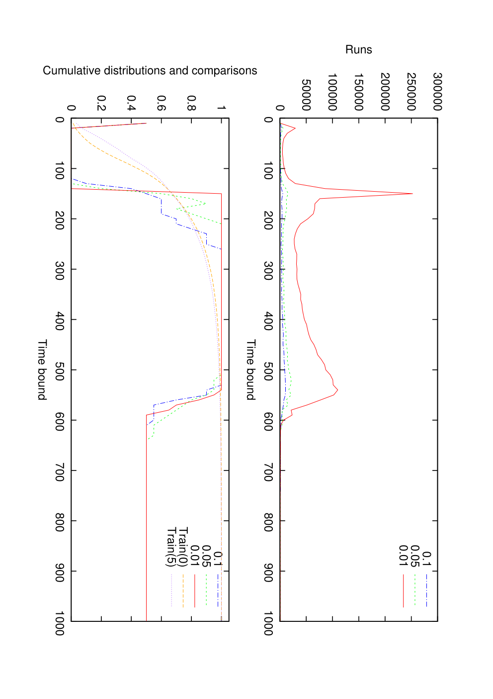
We then compare the probability for Train $0$ to cross when all other trains are stopped with the same probability for Train $5$. In the first plot (Fig. 6 top), we check the same property with $100$ different time bounds from $10$ to $1000$ in steps of $10$ and we plot the number of runs for each check. These experiments only check for the specified bound, they are not parametrised. In the second plot, we use the parametric extension presented in Section V with a granularity of 10 time units. We configured the thresholds $u_{0}$ and $u_{1}$ to differentiate the comparisons at $u_{0}=1-\epsilon$ and $u_{1}=1+\epsilon$ with $\epsilon=0.1,0.05,0.01$ as shown on the figure. In addition, we use a larger time bound to visualise the behaviors after $600$ that are interesting for our checker. In the first plot of Fig. 6, we show for each time bound the average of runs needed by the comparison algorithm repeated 30 times for different values of $\epsilon$. In the bottom plot, we first superpose the cumulative probability for both trains (curves Train 0 and Train 5) that we obtain by applying the quantitative algorithm of Section IV for each time bound in the sampling. Interestingly, before that point, train $5$ is better and later train $0$ is better. Second, we compare these probabilities by using the comparison algorithm (curves 0.1 0.05 0.01). This algorithm can retrieve 3 values: 0 if Train 0 wins, 1 if Train 5 wins and 0.5 otherwise. We report for each time bound and each value of $\epsilon$ the average of these values for 30 executions of the algorithm.

In addition, to evaluate the efficiency of computing all results at once to obtain these curves, we measure the accumulated time to check all the $100$ properties for the first plot (sequential check), and the time to obtain all the results at once (parallel check). The results are shown in Table I. The experiments are done on a Pentium D at 2.4GHz and consume very little memory. The parallel check is about 10 times faster⁵⁵ 5 The implementation checks simulations sequentially using a single thread.. In fact it is limited by the highest number of runs required as shown by the second peak in Fig. 6. The expensive part is to generate the runs so reusing them is important.

Note that at the beginning and at the end, our algorithm aborts the comparison of the curves, which is visible as the number of runs is sharply cut.

The Lightweight Media Access Control (LMAC) protocol is used in sensor networks to schedule communication between nodes. This protocol is targeted for distributed self-configuration, collision avoidance and energy efficiency. In this study we reproduce the improved Uppaal model from [34] without verification optimisations, parametrise with network topology (ring and chain), add probabilistic weights (exponential and uniform) over discrete delay decisions and examine statistical properties which were not possible to check before. Based on [35], our node model consumes 21, 22, 2 and 1 power units per time unit when a node is sending, receiving, listening for messages or being idle respectively.

Fig. 7a shows that collisions may happen in all cases and the probability of collision is higher with exponential decision weights than uniform decision weights, but seems independent of topology (ring or chain). The probability of collision stays stable after 50 time units, despite longer simulations, meaning that the network may stay collision free if the first collisions are avoided. We also applied the method for parametrised probability comparison for the collision probability. The results are that up to 14 time units the probabilities are the same and later exponential weights have higher collision probability than uniform, but the results were inconclusive when comparing different topologies.

The probable collision counts in the chain topology are shown in Fig. 7b, where the case with 0 collisions has a probability of 87.06% and 89.21% when using exponential and uniform weights respectively. The maximum number of probable collisions is 7 for both weight distributions despite very long runs, meaning that the network eventually recovers from collisions.

The probable collision count in the ring topology (not shown) yields that there is no upper bound of collision count as the collisions add up indefinitely, but there is a fixed probability peak at 0 collisions (87.06% and 88.39% using uniform and exponential weights resp.) with a short tail up to 7 collisions (like in Fig. 7b), long interval of 0 probability and then small probability bump (0.35% in total) at large number of collisions. Thus chances of perpetual collisions are tiny.

Fig. 8 shows energy consumption probability density: using uniform and exponential weights in a chain and a ring topologies. Ring topology uses more power (possibly due to collisions), and uniform weights use slightly less energy than exponential weights in these particular topologies.

Duration Probabilistic Automata [19] (DPA) are used for modeling job-shop problems. A DPA consists of several Simple DPAs (SDPA). An SDPA is a processing unit, a clock and a list of tasks to process sequentially. Each task has an associated duration interval, from which its duration is chosen (uniformly). Resources are used to model task races – we allow different resource types and different quantities of each type. A fixed priority scheduler is used to resolve conflicts. A DPA example is shown in Fig. 9.

DPA can be encoded in our tool (with a continuous or discrete time semantics) or in Prism (discrete semantics), see the technical report [36]. In Prism, integer and boolean variables are used to encode the current tasks and resources. Prism only supports the discrete time model. In Uppaal, a chain of waiting and task locations is created for each SDPA. Guards and invariants encode the duration of the task, and an array of integers contain the available resources. The scheduler is encoded as a separate template. We omit the resources and durations from the table for simplicity, they are chosen arbitrarily for the experiment. For Uppaal, both a discrete and continuous time versions have been implemented. The performance of the translations is measured on several case studies and shown in Tables II and III. In the hypothesis testing column, Uppaal (Upp in the table) uses the sequential hypothesis testing introduced in Section IV, whereas Prism uses its own new implementation of the hypothesis testing algorithm. In the estimation column, both Uppaal and Prism use the quantitative check of Section IV, but Uppaal is faster due to implementation details. For both tools, the error bounds used are $\alpha=\beta=0.05$. In the hypothesis test, the indifference region size is $0.01$, while we have $\epsilon=0.05$ for the quantitative approach. The results show that Uppaal is faster than Prism even with the discrete encoding, which currently is the only fair comparison.

In the first test, we create a DPA with $n$ SDPAs, $k$ tasks per SDPA and no resources. The duration interval of each task is changed and the verification time is measured. In the second test, we choose $n$, $k$ and let $m$ be the number of resource types. The resource usage and duration intervals are randomised. The query for the approximation test is: “What is the probability of all SDPAs ending within $t$ time units?”. In the verification test, we ask the query: “Do all SDPAs end within $t$ time units with probability greater than 40%?”. The value of $t$ varies for each model as it was computed by simulating the system 369 times and represent the value for which at least 60% of the runs reached the final state.

References

- [1] E. Clarke, O. Grumberg, and D. Peled, Model Checking. MIT Press, 1999.
- [2] R. Alur and D. Dill, “A Theory of Timed Automata,” Theoretical Computer Science, vol. 126, pp. 183–235, 1994.
- [3] R. Alur, C. Courcoubetis, N. Halbwachs, T. A. Henzinger, P. Ho, X. Nicollin, A. Olivero, J. Sifakis, and S. Yovine, “The algorithmic analysis of hybrid systems,” Theoretical Computer Science, vol. 138, no. 1, pp. 3–34, 1995.
- [4] G. Behrmann, A. Fehnker, T. Hune, K. G. Larsen, P. Pettersson, J. Romijn, and F. W. Vaandrager, “Minimum-cost reachability for priced timed automata,” in HSCC, ser. LNCS, M. D. D. Benedetto and A. L. Sangiovanni-Vincentelli, Eds., vol. 2034. Springer, 2001, pp. 147–161.
- [5] R. Alur, S. L. Torre, and G. J. Pappas, “Optimal paths in weighted timed automata,” in HSCC, ser. LNCS, M. D. D. Benedetto and A. L. Sangiovanni-Vincentelli, Eds., vol. 2034. Springer, 2001, pp. 49–62.
- [6] “The spin tool (spin),” available at http://spinroot.com/spin/whatispin.html.
- [7] “The smv model checker,” available at http://www.kenmcmil.com/smv.html .
- [8] “The uppaal tool,” available at http://www.uppaal.com/.
- [9] G. Frehse, “Phaver: algorithmic verification of hybrid systems past hytech,” STTT, vol. 10, no. 3, pp. 263–279, 2008.
- [10] C. Baier, N. Bertrand, P. Bouyer, T. Brihaye, and M. Größer, “Probabilistic and topological semantics for timed automata,” in FSTTCS, ser. LNCS, vol. 4855. Springer, 2007, pp. 179–191.
- [11] N. Bertrand, P. Bouyer, T. Brihaye, and N. Markey, “Quantitative model-checking of one-clock timed automata under probabilistic semantics,” in QEST. IEEE Computer Society, 2008, pp. 55–64.
- [12] H. Bohnenkamp, P. D’Argenio, H. Hermanns, and J.-P. Katoen, “Modest: A compositional modeling formalism for real-time and stochastic systems,” University of Twente, Technical Report CTIT 04-46, 2004.
- [13] T. Teige, A. Eggers, and M. Fränzle, “Constraint-based analysis of concurrent probabilistic hybrid systems: An application to networked automation systems,” Nonlinear Analysis: Hybrid Systems, 2011.
- [14] H. L. S. Younes, “Verification and planning for stochastic processes with asynchronous events,” Ph.D. dissertation, Carnegie Mellon, 2005.
- [15] K. Sen, M. Viswanathan, and G. Agha, “Statistical model checking of black-box probabilistic systems,” in CAV, ser. LNCS 3114. Springer, 2004, pp. 202–215.
- [16] R. Wald, Sequential Analysis. Dove Publisher, 2004.
- [17] T. Hérault, R. Lassaigne, F. Magniette, and S. Peyronnet, “Approximate probabilistic model checking,” in VMCAI, ser. LNCS, 2004, pp. 73–84.
- [18] A. David, K. Larsen, A. Legay, Z.Wang, and M. Mikucionis, “Time for real statistical model-checking: Statistical model-checking for real-time systems,” in CAV, ser. LNCS. Springer, 2011.
- [19] O. Maler, K. G. Larsen, and B. H. Krogh, “On zone-based analysis of duration probabilistic automata,” in INFINITY, ser. EPTCS, vol. 39, 2010, pp. 33–46.
- [20] K. G. Larsen and A. Skou, “Bisimulation through probabilistic testing,” in POPL, 1989, pp. 344–352.
- [21] H. L. S. Younes and R. G. Simmons, “Probabilistic verification of discrete event systems using acceptance sampling,” in CAV, ser. LNCS 2404. Springer, 2002, pp. 223–235.
- [22] H. L. S. Younes, “Ymer: A statistical model checker,” in CAV, ser. LNCS, vol. 3576. Springer, 2005, pp. 429–433.
- [23] P. Zuliani, A. Platzer, and E. M. Clarke, “Bayesian statistical model checking with application to simulink/stateflow verification,” in HSCC. ACM ACM, 2010, pp. 243–252.
- [24] S. K. Jha, E. M. Clarke, C. J. Langmead, A. Legay, A. Platzer, and P. Zuliani, “A bayesian approach to model checking biological systems,” in CMSB, ser. LNCS, vol. 5688. Springer, 2009, pp. 218–234.
- [25] E. M. Clarke, A. Donzé, and A. Legay, “Statistical model checking of mixed-analog circuits with an application to a third order delta-sigma modulator,” in HVC, ser. LNCS, vol. 5394. Springer, 2008, pp. 149–163.
- [26] J. Bogdoll, L.-M. Fiorti, A. Hartmanns, and H. Hermanns, “Partial order methods for statistical model checking and simulation,” in FORTE, ser. LNCS. Springer, 2011, to appear.
- [27] M. Minea, “Partial order reduction for verification of timed systems,” Ph.D. dissertation, Carnegie Mellon, 1999.
- [28] K. Sen, M. Viswanathan, and G. Agha, “On statistical model checking of stochastic systems,” in CAV, ser. LNCS 3576, 2005, pp. 266–280.
- [29] A. Basu, S. Bensalem, M. Bozga, B. Caillaud, B. Delahaye, and A. Legay, “Statistical abstraction and model-checking of large heterogeneous systems,” in FORTE, ser. LNCS, vol. 6117. Springer, 2010, pp. 32–46.
- [30] A. David, K. Larsen, A. Legay, U. Nyman, and A. Wasowski, “Timed I/O automata: a complete specification theory for real-time systems,” in HSCC. ACM, 2010.
- [31] P. Panangaden, Labelled Markov Processes. Imperial College Press, 2010.
- [32] T. Hérault, R. Lassaigne, F. Magniette, and S. Peyronnet, “Approximate probabilistic model checking,” in VMCAI, ser. LNCS, vol. 2937. Springer, 2003, pp. 307–329.
- [33] G. Behrmann, A. David, and K. G. Larsen, “A tutorial on Uppaal,” in SFM, ser. ncs(3185), M. Bernardo and F. Corradini, Eds. Springer, 2004, pp. 200–236.
- [34] A. Fehnker, L. van Hoesel, and A. Mader, “Modelling and verification of the lmac protocol for wireless sensor networks,” in Integrated Formal Methods, ser. LNCS, J. Davies and J. Gibbons, Eds. Springer Berlin / Heidelberg, 2007, vol. 4591, pp. 253–272.
- [35] L. F. W. van Hoesel, “Sensors on speaking terms: schedule-based medium access control protocols for wireless sensor networks,” Ph.D. dissertation, University of Twente, June 2007. [Online]. Available: http://doc.utwente.nl/57885/
- [36] D. Poulsen and J. van Vliet, “Duration probabilistic automata,” Aalborg University, Tech. Rep., 2011.
- [37] J. Bucklew, Introduction to Rare event Simulation. Springer, 2004.
- [38] D. E. Rabih and N. Pekergin, “Statistical model checking using perfect simulation,” in ATVA, ser. LNCS, vol. 5799. Springer, 2009, pp. 120–134.
- [39] J.-P. Katoen and I. S. Zapreev, “Simulation-based ctmc model checking: An empirical evaluation,” in QEST. IEEE, 2009, pp. 31–40.
- [40] H. L. S. Younes, E. M. Clarke, and P. Zuliani, “Statistical verification of probabilistic properties with unbounded until,” in SBMF, ser. LNCS, vol. 6527. Springer, 2010, pp. 144–160.
- [41] P. Ballarini, H. Djafri, M. Duflot, S. Haddad, and N. Pekergin, “HASL: An expressive language for statistical verification of stochastic models,” in VALUETOOLS), May 2011, to appear.
- [42] M. D. D. Benedetto and A. L. Sangiovanni-Vincentelli, Eds., Hybrid Systems: Computation and Control, 4th International Workshop, HSCC 2001, Proceedings, ser. LNCS, vol. 2034. Springer, 2001.