$\begin{array}[]{lll}\mbox{Prof.}&\mbox{Geneviève B\'{e}langer}&\mbox{Rapporteur}\\ \mbox{Prof.}&\mbox{Lars Bergström}&\mbox{Rapporteur}\\ \mbox{Prof.}&\mbox{Abdelhak Djouadi}&\mbox{Directeur de Thèse}\\ \mbox{Prof.}&\mbox{Ulrich Ellwanger}&\mbox{Président du jury}\\ \mbox{Prof.}&\mbox{Yann Mambrini}&\mbox{Membre invité du jury}\\ \mbox{Prof.}&\mbox{Aldo Morselli}&\mbox{Membre du jury}\\ \mbox{Prof.}&\mbox{Carlos Mu\~{n}oz}&\mbox{Membre du jury}\\ \end{array}$

Aux batailles qu’on a donné
et à celles qui viennent.

[Uncaptioned image]

UNIVERSITÉ PARIS-SUD 11

THÈSE DE DOCTORAT

Spécialité: PHYSIQUE THÉORIQUE

Présentée

pour obtenir le grade de

Docteur de l’Université Paris - Sud

par

Andreas Goudelis

Detection of WIMP-like dark matter in some
extensions of the Standard Model

$\begin{array}[]{lll}\mbox{Prof.}&\mbox{Geneviève B\'{e}langer}&\mbox{Rapporteuse}\\ \mbox{Prof.}&\mbox{Lars Bergström}&\mbox{Rapporteur}\\ \mbox{Prof.}&\mbox{Abdelhak Djouadi}&\mbox{Directeur de Thèse}\\ \mbox{Prof.}&\mbox{Ulrich Ellwanger}&\mbox{Président du jury}\\ \mbox{Prof.}&\mbox{Yann Mambrini}&\mbox{Membre invité du jury}\\ \mbox{Prof.}&\mbox{Aldo Morselli}&\mbox{Membre du jury}\\ \mbox{Prof.}&\mbox{Carlos Mu\~{n}oz}&\mbox{Membre du jury}\\ \end{array}$

Introduction et sommaire

Ce travail traite la détection de la matière noire dans quelques extensions du Modèle Standard de la physique des particules. Avant de se lancer dans la partie la plus technique, il serait peut - être pertinent de résumer l’idée principale derrière le concept de la matière noire.

Aujourd’hui les physiciens disposent d’une série des lois physiques qui peuvent fournir des cadres de description des intéractions entre des objets massifs. Ces lois sont la Relativité Générale et la mécanique Newtonienne. Ces théories peuvent, entre autres, relier trois choses: la masse d’un objet, celles des objets de son entourage ainsi que son comportement cinématique (la manière dont il bouge). Si on peut mesurer deux parmi ces trois quantités, nous pouvons en principe prédire la troisième. Si nous pouvons mesurer toutes les trois quantités, nous pouvons en tirer des conclusions concernant la validité de la théorie.

Ces deux théories ont effectivement eu un succès énorme pour expliquer toute une série de phénomènes, comme le mouvement des objets planétaires dans le système solaire, le mouvement des objets au voisinage de la terre, bref, un grand nombre des phénomènes où la gravitation est suffisament forte pour qu’elle puisse jouer un rôle important.

Supposons pourtant qu’il s’avère que des situations apparaissent où si on mesure la masse d’un objet et celle des objets qui l’entourent, le comportement cinématique prévu par la théorie est en désaccord avec celui qui est observé. Dans un tel cas, il nous reste deux solutions:

•

On pourrait admettre que nous sommes arrivés aux limites de validité de notre théorie et essayer de modifier sa formulation ou son context conceptuel.
•

Ou il faut admettre que les observations sont elles-mêmes, dans un sens, problématiques: Ça peut être que nous avons mal mesuré la masse de l’objet observé, la masse des objets qui l’entourent ou sa trajectoire dans le ciel. Autrement dit, nous avons peut être utilisé “les bonnes équations” mais pas les bonnes quantités dans ces équations.

Si nous ne souhaitons pas modifier la forme des théories de la gravitation (malgré le fait qu’une telle approche est souvent adoptée par plusieurs chercheurs et groupes, avec des resultats très intéressants), il nous reste que la deuxième option. Il y a pourtant plusieures raisons pour croire que les mesures de masse et de comportement cinématique sont assez fiables ¹¹ 1 Il est pourtant assez intéressant que la première mesure relative était, en fait, fausse!. On pourrait donc supposer avec une certaine confiance que les mesures concernant les objets qu’on voit ne sont pas fausses. Il semble alors qu’on arrive à une impasse. On pourrait dans un tel cas supposer qu’il existe quelques objets qu’on ne peut pas voir effectivement mais qui devraient être pris en compte en tant qu’objets “d’entourage” afin de prédire correctement le comportement cinématique de l’objet qu’on observe. Cela a été le premier argument pour le postulat de la matière noire.

Il s’avère qu’adopter une telle solution n’est pas quelque chose de nouveau en physique: la planète de Pluto (qui n’a aujourd’hui rien de mystique pour les astrophysiciens) a été prédite pour la première fois sans être visible à l’époque grâce à des anomalies dans le mouvement des objets planétaires. L’existence des neutrinos (expérimentalement bien - établie aujourd’hui) a été postulée car la lois de la conservation de l’énergie totale d’un système était menacée dans les observations des désintégrations radioactives de quelques noyaux. La matière noire a été introduite de façon similaire, à la suite d’observations astronomiques à differentes échelles.

Mais que se passe-t-il s’il se trouve que cette matière noire ne peut pas être constituée par la forme de matière connue? Dans ce cas, on pourrait dire que l’histoire devient encore plus interessante! Pourrait-on espérer observer cette nouvelle matière un jour? Cela dépend fortement de sa nature, et est un des sujets principaux de ce travail.

Il existe plusieurs façons (complémentaires) de traiter la matière noire. Dans cette thèse, nous nous focaliserons sur l’approche de la physique des particules, en introduisant pourtant des élements d’astrophysique et de cosmologie (cette division est déjà assez brutale).

Le premier chapitre du travail ci-dessous présente brièvement quelques élements de base qui sont indispensables pour travailler sur la matière noire. Nous allons présenter quelques éléments de formalisme de Relativité Générale et de cosmologie, puis décrire plus en détail quelques arguments pour le postulat de la matière noire. Une petite discussion suit sur les caractéristiques possibles de la matière noire et l’incapacité du Modèle Standard de fournir un candidat viable.

Dans le deuxième chapitre nous discutons sur les modes de détection de la matière noire. Après une présentation des modes principaux de détection (au moins ceux qui existent aujourd’hui), nous expliquons quelques incertitudes qui entrent dans chaque canal de détection et nous présentons brièvement la situation experimentalle actuelle. Ensuite nous décrivons quelques resultats originaux sur la capacité des experiences à reconstruire quelques propriétés des candidats pour la matière noire.

Au troisième chapitre nous décrivons une solution minimale au problème de la matière noire. Le Modèle Standard de la physique des particules est légèrement étendu pour inclure une particule qui pourrait constituer la masse manquante de l’univers. Après une description du modèle et une étude de quelques unes de ses propriétés et contraintes, nous discutons ses perspctives de détection en montrant qu’il pourrait être testé auprès des expériences courrantes ou à venir.

Dans le quatrième chapitre, nous présentons une deuxième solution au problème de la matière noire. Cette fois, l’approche est beaucoup moins minimale et économique et les modèles qui en découlent sont considérablement plus compliqués. Pourtant, cette approche (appellée sypersymétrie) présente l’avantage d’avoir été motivée par des questions tout à fait différentes, l’existence d’un candidat de matière noire étant une conséquence des considérations plus génériques. Nous présentons quelques éléments de formalisme supersymétrique et puis la version minimale de cette sorte des théories, ainsi qu’un des candidats qu’elle propose. Ensuite, nous discutons d’un problème spécifique qui apparaît dans ce modèle et nous étudions la matière noire dans deux modèles qui essayent de resoudre ce problème.

Finalement, un resumé et la conclusion forment un cinquième chapitre. Trois appendices suivent, qui contiennent quelques éléments techniques ainsi qu’un certain nombre des points qui renforcent quelques arguments qui sont donnés dans le corps du texte.

Paris, printemps/été 2010

Introduction and summary

This work treats the detection of dark matter in some extensions of the Standard Model of particle physics. Before starting with the more technical part of this work, it could perhaps be pertinent to summarize the main idea behind the concept dark matter.

Today physicists have at their disposal a series of “physical laws” that provide frameworks to describe the interactions between massive objects. These laws are General Relativity and Newtonian mechanics. Among others, these physical theories can relate three things: the mass of an object, that of its surrounding ones, as well as the kinematic behavior that we would expect this object to follow (how it should move). If we can measure two of these quantities, we can in principle predict the third one or, seen a bit differently, if we can measure all three of them we can draw conclusions on the validity of these theories.

Indeed, these two theories have been extremely successful in explaining a very large amount of phenomena, such as the motion of planets in the solar system, the motion of objects close to the earth, in short, a huge variety of phenomena where gravitational interactions are strong enough play a significant role.

Suppose however that it turns out that there are some cases where if we somehow measure the mass of an object and of its surrounding ones, the predicted kinematic behavior is in conflict with the observed one. In this case, we are left with more or less two options:

•

We could admit that the limits of validity of the theories at our disposal have been reached, and try to modify our theories’ formulation, or conceptual content,
•

Or we must admit that the observations are themselves, in some sense, problematic, where by this we mean that we could have mismeasured the mass of the observed object, the mass of its surrounding objects or its trajectory in the sky. In other words, it could be that we used “the correct formulae” but we did not plug the correct quantities in these formulae.

In practice, if we wish not to alter the form of current theories of gravitation (although such an approach is also adopted by several researchers and groups, with very interesting results), we are stuck with the second option. Now, there are several reasons that allow one to believe that mass and kinematic behavior measurements can be quite reliable ²² 2 It is though quite interesting that the first relevant measurement was actually false!. So, it could be supposed quite safely that the measurements concerning the things we see are not false. The situation seems thus to reach some sort of impass. We could then assume that there are some objects that we cannot currently see and which should be taken into account as “surrounding objects” in order to correctly predict the kinematic behavior of the object under observation. This was the first argument that lead to the dark matter postulate.

It turns out that resorting to such a solution is not something new in physics: The planet Pluto (which today has nothing mystical for astrophysicists) was first predicted without being visible at the time due to anomalies in the movement of planetary objects. The existence of neutrinos (which is experimentally well - established today) was postulated because the law of conservation of the total energy of a system was put in hazard when observing radioactive decays of some nuclei. It is in a similar manner that dark matter was introduced, receiving as we shall see in the following increasingly strong support from other observational evidence.

But what if it turns out that this dark matter cannot be constituted by the known matter forms? Well, in this case, one could say that things get even more interesting! Could we hope one day to actually see this new matter? This depends strongly on its nature, and this is one of the main topics in this work.

There are actually many (complementary) ways of tackling dark matter. In this work, we shall focus on the approach of particle physics, introducing however elements of astrophysics and cosmology (this division is already quite brutal).

The first chapter of this work briefly presents some background material needed to work with dark matter. We shall present some elements of formalism of General Relativity and cosmology, then describe some motivation that lead to the dark matter postulate. A brief discussion follows on the possible characteristics of dark matter and the incapacity of the Standard Model of particle physics to accommodate some “viable candidate”.

In the second chapter we start discussing how dark matter could be detected. After presenting the main methods of dark matter detection (at least those existing today), we further explain some of the uncertainties entering each detection mode and briefly present the current status of the field. We then present some original results on the capacity of the corresponding experiments to reconstruct some properties of dark matter candidates.

In the third chapter we describe a minimal approach towards the dark matter problem. The Standard Model of particle physics is slightly extended so as to incorporate a particle that could account for the missing matter content of the universe. After describing the model and examining some aspects of its constraints and phenomenology, we discuss its detection perspectives showing that we could expect it to be tested in present or oncoming experiments.

In the fourth chapter we describe another solution to the dark matter problem. This time the approach is much less minimal and economic, with the corresponding models being considerably more complicated. However, this approach (called supersymmetry) presents the merit of having been motivated from completely different questions, with the dark matter candidate particle arising quite naturally as a consequence of more generic considerations. We present some elements of supersymmetric formalism and then the minimal version of such theories along with one of the potential dark matter candidates it proposes. Then, we discuss a particular problem arising in this model and treat dark matter in two examples of models trying to tackle this issue.

Finally, we summarize and conclude in the fifth chapter. Three appendices contain some technical elements used throughout this work as well as some points aiming at corroborating certain arguments given in the main body of the text.

Paris, spring/summer 2010

Chapter 1 The two Standard Models

One of the main issues in today’s high energy physics is the almost complete absence of experimental evidence of new physics. It turns out, however, that in trying to combine our knowledge in the field of physics at very small scales (particle physics) and physics at very large ones (cosmology), the necessity to go beyond one of them arises. In this chapter, we shall introduce the two “standard pictures” for the respective fields and explain how they turn out to be insufficient in order to explain today’s observations.

1.1 A basic observation

Looking at the sky and asking questions about “everything there is” is not a new habit. People have been engaging themselves into this enterprise since a very long time. It is in fact partly by observing motions of extraterrestrial objects that we understood that everything in this world seems to be moving with respect to other things. In the beginning, of course, at least to our knowledge, there is one object which was considered to be completely inert, the earth. With time, when the world came to position of being able to overcome the Aristotelean approach towards nature, it was gradually understood that in fact our planet is also in constant motion.

Despite this fundamental understanding, though, it took quite some more time for another basic breakthrough in our way of thinking to be established. Even with the rise of Newtonian (and then Lagrangian and Hamiltonian) mechanics, the mechanistic approach towards reality suggested that extremely complex phenomena can take place in our world, but which actually happen in an otherwise inert, constant, eternal environment, space: a field is something that propagates through space, even perhaps with a limited velocity, but space itself does not play a crucial role in the process. It could perhaps, like in the Aristotelean theory, acquire some properties, but its form always remained the same.

It is not until the twentieth century that scientists started wondering about the role of space (-time) in physical phenomena. And it is not until the introduction of General Relativity that spacetime started being conceived as something which is actually bound to the phenomena taking place “inside” it: The action of a gravitational field is now understood as a deformation of spacetime.

At the same time, the development of quantum mechanics contributed further to the demolition of this mechanistic view of our world. More on this shall be said in the following, when we describe the standard model of particle physics.

Once we start believing that spacetime is a dynamical object, which can change and participate actively in physical processes, a question that could rise is whether spacetime is something finite. And, according to our current perceptions, it actually is. A number of observations have contributed to this evolution in our concepts, which are actually often said to consist the basis of modern cosmology.

The first observation is that the universe (including spacetime) seems to be actually expanding with time. If this is the case (and today we are quite confident that it is), this means that if we try to trace its evolution throughout time it is necessary to develop the appropriate notions and formalism in order to be able to treat phenomena taking place in such an environment. And, if the universe has been expanding up to its current size for quite some time, an immediate question is how could it look at much earlier times, when its size was much smaller than today. The belief that the total amount of energy and matter (unified already in special relativity) stays constant, i.e. that there is no creation or eradication of these two in the universe (since the “universe” is a closed thermodynamical system, it’s simply “everything there is”) could probably make us hope that we can trace back what the place we live in looked like in past times. In the next section, we shall introduce some of these notions and formalisms.

1.2 Elements of General Relativity

One of the main questions that arise in an expanding universe (but which has much more far-reaching consequences) is how to relate physical and coordinate distances [1, 2, 3]. This is actually achieved through the introduction of the metric of the space, $g_{\mu\nu}$ , through:

ds^{2}=g_{\mu\nu}dx^{\mu}dx^{\nu}

(1.1)

where summation over repeated indices is implied.
The distance $s$ is invariant in every coordinate system, whereas in the above equation the metric connects the values of coordinates to the more physical measure of the interval $ds$ .

As we shall shortly describe, General Relativity relates the presence of matter to deformations of the spacetime metric. In the special case where there is no matter in space spacetime is flat, the metric is the Minkowski one and particles move in straight lines. Now, in a curved manifold, particles moving freely will no longer follow straight lines but rather more complex trajectories, called geodesics. The equations of motion in curved spacetime acquire, in their turn, also a more complicated form, which is

\frac{d^{2}x^{\mu}}{d\lambda^{2}}=-\Gamma^{\mu}_{\alpha\beta}\frac{dx^{\alpha}}{d\lambda}\frac{dx^{\beta}}{d\lambda}

(1.2)

where $\lambda$ is some monotonically increasing parameter along the particles’ path (which can always be eliminated in actual calculations) whereas $\Gamma^{\mu}_{\alpha\beta}$ are the Christoffel symbols, defined as

\Gamma^{\mu}_{\alpha\beta}=\frac{1}{2}g^{\mu\nu}(\partial_{\beta}g_{\alpha\nu}+\partial_{\alpha}g_{\beta\nu}-\partial_{\nu}g_{\alpha\beta})

(1.3)

Now, since we said that the universe is expanding, an important question is the way this should be reflected in the metric. Actually, for a flat spacetime, the metric in an expanding universe is given by the famous Friedmann-Robertson-Walker-Lemaître (FLRW) formula

g_{\mu\nu}=\left(\begin{array}[]{cccc}-1&0&0&0\\ 0&a^{2}(t)&0&0\\ 0&0&a^{2}(t)&0\\ 0&0&0&a^{2}(t)\end{array}\right)

(1.4)

where $a(t)$ is a function of time, called the scale factor, which describes the evolution of distances with time: if the comoving distance between two points at some time is $1$ , at later times it will be $a(t)>1$ . Its present value is set to $1$ and it increases with time.

There is a fundamental consequence of the FLRW metric. If we start with a particle of $4$ - momentum $p^{\alpha}=(E,\vec{p})$ and define the $\lambda$ parameter through $p^{\alpha}=dx^{\alpha}/d\lambda$ then we can easily demonstrate that the energy of the particle decreases with time (i.e. with the expansion of the universe). This observation finds its physical interpretation in the fact that as the universe expands, and all distances become larger, the wavelength of the particle also stretches decreasing its energy.

At the center of General Relativity lies the observation that the metric can account for gravitational phenomena. This is done through the Einstein equation

G_{\mu\nu}=R_{\mu\nu}-\frac{1}{2}g_{\mu\nu}R=8\pi GT_{\mu\nu}

(1.5)

where $G_{\mu\nu}$ is called the Einstein tensor, $R_{\mu\nu}$ is the Ricci tensor defined as

R_{\mu\nu}=\Gamma^{\alpha}_{\mu\nu,\alpha}-\Gamma^{\alpha}_{\mu\alpha,\nu}+\Gamma^{\alpha}_{\beta\alpha}\Gamma^{\beta}_{\mu\nu}-\Gamma^{\alpha}_{\beta\nu}\Gamma^{\beta}_{\mu\alpha}

(1.6)

with $,\alpha$ denoting derivation with respect to $x^{\alpha}$ , $R$ is the Ricci scalar defined as the contraction of the Ricci tensor with the metric, $G$ is the Newton constant whereas $T_{\mu\nu}$ is the energy-momentum tensor. Eq.(1.5) introduces a clear correlation among the matter-energy content of spacetime and its geometry: what would be called in Newtonian terms “gravitational force” is actually the effect of the deformation of spacetime and the consequent modification in the particles’ trajectories.

In the LHS of Eq.(1.5) one can also add a term of the form $\Lambda g_{\mu\nu}$ , called the cosmological constant term, with enormous consequences that we shall not be examining here. Let us just note for the moment that this term can be used in order to explain the accelerating expansion of the universe and is responsible for the so-called “dark energy” which seems to be the main component of the matter-energy content of our universe.

Now, observations at large scales seem to favor a couple of very fundamental assumptions, namely that the universe is homogeneous and isotropic. The first assumption means that for sufficiently large volumes (and we shall comment on that in the following) the density of the universe is the same no matter in which region we consider the volume. The second assumption means that there should be no privileged direction in the universe.

It turns out that these two basic assumptions constrain enormously the possibilities to consider different metrics as solutions to the Einstein equations. The most general form of the metric compatible with the two assumptions can actually be written, in spherical coordinates, as:

ds^{2}=-dt^{2}+a(t)^{2}\left[\frac{dr^{2}}{1-kr^{2}}+r^{2}(d\theta^{2}+\sin^{2}\theta d\phi^{2})\right]

(1.7)

where $k$ takes the values $-1,0,1$ for a universe with negative, zero or positive curvature respectively. We note that the spatial part of the metric has a dependence on time. This is actually a generalization of the FLRW metric that we wrote down before.

A question arises on the form of the energy-momentum tensor. In cosmology, the matter-energy content of the universe (encoded exactly by the energy-momentum tensor) is usually taken to behave (at sufficiently large scales) as a perfect fluid. In this case, $T_{\mu\nu}$ takes the form

T_{\mu\nu}=\mbox{diag}(\rho,p,p,p)

(1.8)

where $\rho$ is the fluid’s density and p is its pressure.

It is not that difficult to see that by taking the time component of the Einstein equation, we should get a relation between the matter-energy density of the universe and the scale factor. In fact, this relation is

H^{2}(t)\equiv\left(\frac{\dot{a}(t)}{a(t)}\right)=\frac{8\pi G\rho}{3}-\frac{k}{a^{2}(t)}

(1.9)

which is called the Friedmann equation.

Furthermore, the continuity relation for the fluid yields

\frac{d(\rho a^{3})}{dt}=-p\frac{d(a^{3})}{dt}

(1.10)

Now, define the critical density of the universe as

\rho_{c}\equiv\frac{3H^{2}}{8\pi G}.

(1.11)

The value of this parameter determines whether the universe expands forever or eventually collapses to a singularity once more ¹¹ 1 The presence of the cosmological constant term complicates the situation, but this detail goes beyond the scope of the present work..

Then, by further defining normalized densities $\Omega\equiv\rho/\rho_{c}$ , $\Omega_{\Lambda}\equiv\Lambda/(8\pi G\rho_{c})$ and $\Omega_{k}\equiv-k/\dot{a}^{2}$ for the energy-matter, dark energy and curvature densities respectively, we can bring the Friedmann equation to a very simple form

\Omega+\Omega_{\Lambda}+\Omega_{k}=1

(1.12)

With these tools at hand, we can in principle examine the evolution of all of the universe’s components with time during its expansion. We should stress at this point that since the Einstein equations are obviously linear with the energy-momentum tensor, one could (at least as far as gravitational interactions are concerned) separate the various contributions and examine their evolution in an uncorrelated manner.

Finally, so far we have considered that the cosmic fluid is perfectly homogeneous. However, global homogeneity does not impose that locally there cannot be small inhomogeneities. The usual approach is to actually consider the “vacuum” state as being the perfectly isotropic and homogeneous one, then adding perturbations around the ground state metric and examining the evolution with time. The very existence of structures in our universe (planets, stars, galaxies, clusters of galaxies) is a witness that inhomogeneities must have existed. These do actually exist and we can today see their footprints in the Cosmic Microwave Background (CMB) radiation anisotropies.

1.3 Evidence for Dark Matter

1.3.1 Galactic Rotation Curves

According to our previous discussion, once one knows the matter content of some gravitating system, one should be able to write down its equations of motion and predict its kinematic behavior. Actually, in the cases of vanishing curvature (as for example when examining a galaxy as a whole) then even simple Newtonian mechanics should be sufficient to fulfill this task. Inversely, by observing the kinematic behavior of a gravitating system, we should be able to determine its matter content. Departures from the behavior predicted by the theory should either be explained by a modification in the relation among the dynamics and the matter content of the system, or by a modification in the matter content itself.

This was actually one of the first arguments supporting the existence of some form of (yet, as we shall argue in the following chapters) invisible matter. ²² 2 Several reviews on (particle) dark matter exist. See, for example, [4, 5, 6, 7] According to Newtonian mechanics, the circular velocity of the gas and the stars comprising a galaxy as a function of the distance from the galactic center is given by the very simple formula

v(r)=\sqrt{\frac{GM(r)}{r}}

(1.13)

where $v$ is the velocity at distance $r$ from the center of the galaxy and $M$ is the mass enclosed in a sphere of radius $r$ . From this simple relation, even accepting that in reality things could be slightly more complex, one would expect that once we move far enough from the galactic center, where we can say quite confidently from observations of the luminous components that we have included in $M(r)$ the essential part of the galaxy’s mass, we would expect a velocity falling roughly as $1/\sqrt{r}$ . It turns out that very often this is not at all the case.

In fig.1.1 we see the rotation curve for the spiral galaxy NGC $6503$ and the various velocity distributions as a function of the distance from the galaxy’s center.

Refer to caption — Figure 1.1: Rotation curve of NGC 6503. The dotted, dashed and dash-dotted lines are the contributions of gas, disk and dark matter, respectively. Figure taken from [5].

We clearly see an unexpected behavior, with the the overall velocity following a flat distribution at large distances from the luminous disk. This behavior suggests that either there should be some modification of the laws of gravity at the galactic scales, or that there is some important (in fact, dominant) quantity of some sort of matter that has persistently evaded detection. We shall be referring, according to habits, to such a matter as being “dark”, i.e. non-luminous.

We should of course notice that both explanations seem equally reasonable at this stage. Although throughout this work we shall be examining some possible consequences of the latter possibility, there is extensive research since quite some time in the field of potential modifications of gravity: Modified Newtonian Dynamics (MOND), Tensor-Vector-Scalar (TeVeS) theories as relativistic versions of the former, $f(R)$ theories etc. And, certainly, one cannot exclude that the solution lies somewhere in between. Finally, it has also been argued that once we depart from the fluid approach for the various components of the universe and start taking into account granular structure, results could be severely altered (although such approaches have not been examined as thoroughly) [8].

1.3.2 Gravitational Lensing

Important evidence for the existence of either some form or non-luminous matter or some modification of gravity comes equally from gravitational lensing experiments. Here, we observe the way light bends under the influence of gravitational potentials as it passes by massive objects. So, for example, an object “behind” (with respect to us) a galaxy cluster emitting light shall be seen distorted with respect to its original shape. By observing this distortion effect, we can infer information on the distribution of matter in space. It turns out that quite often, by only taking into account luminous matter, it is not possible to explain such effects.

One of the most compelling evidence for the existence of dark matter came recently with weak lensing observations of the Bullet galaxy cluster (1E 0657-56) [9] by the Hubble space telescope. The Bullet cluster consists of two colliding galaxy clusters. These, in their turn, have two main components, namely stars and dust/gas. One would expect that upon collision the star components of the two clusters would not be significantly slowed down, since they practically do not interact among them. On the other hand, the intergalactic gas, which is the major component of the cluster’s luminous matter, does interact electromagnetically and should thus be significantly slowed down during the collision. This is actually the case. This can be seen in fig.1.2. In the left hand-side image we see the star content of the two clusters which is well separated after the collision.

The dust component on the other hand, which can be seen in the right hand-side figure in $X$ -rays (mostly concentrated around the yellow regions), seems not to follow the same behavior, being concentrated mostly around the “collision center”. Then, since the gas constitutes the main component of the two clusters, the overall matter distribution for the Bullet cluster, depicted in the images by the mass density contours in green, should follow its behavior. However, we see that this is clearly not the case. On the contrary, the matter density seems to be following a behavior that resembles significantly to the one of stars. This means that there should be some important, actually largely dominant, amount of matter that is unobservable for the moment and drives the matter density distribution in the cluster. This matter should also be quite collisionless, since if it interacted strongly (apart from the fact that it would have probably been observed as such), it would at least behave in a way qualitatively similar to the gas. We note that this is considered to be one of the main observations favoring the dark matter interpretation against the modified gravity one, since gravity (at least according to our current perceptions) does not distinguish among matter forms.

We should note that at the scale of galaxy clusters, many more observations advocate for the existence of dark matter, although quite often alternative approaches can also explain relevant data. In these cases, a quite large number of observations can be made, mainly relevant to the observed temperature of the clusters, and compared against the expected temperature as a function of the cluster’s mass. Alternatively, one can compare the mass of the cluster as observed in all wavelengths against data from weak gravitational lensing. In most cases, a severe discrepancy is found among calculation and observations, supporting the existence of a significant amount of dark matter.

1.3.3 The Cosmic Microwave Background

Many more observations support the idea that there is something wrong in the Einstein equations, either concerning their general form (modifications of gravity) or the matter content we should plug in these equations in order to perform calculations. It is not our goal to list all of this evidence at this point. We could not, however, omit one of the most important observations of modern cosmology, namely the anisotropies of the Cosmic Microwave Background radiation.

The existence of the CMB was first predicted by Gamow in 1948 and further established experimentally by the work of Penzias and Wilson in 1965. Giving a more or less complete description of the CMB-related theory and phenomenology goes well beyond the scope of the present work. The main idea is that once the universe cooled down sufficiently, the photons could no longer interact with matter (matter - radiation decoupling) in an efficient way. Then, as we saw, expansion tends to “stretch” the wavelengths of photons, leading to an overall cooling of this “relic” radiation.

At first, what was observed is a practically perfect blackbody radiation, consisting exactly of these photons as predicted. With the measurements of COBE and especially the WMAP mission, it was realized that although the CMB appears to globally isotropic and homogeneous, at smaller scales there are small but measurable anisotropies in this radiation.

The standard picture today is that small inhomogeneities - perturbations around the ground state metric result in gravitational wells and hills. Then, the rest of the matter-energy content of the universe feels these gravitational wells and tends to cluster around them. As time passes by, the -initially small- perturbations grow and structures (gravitationally bound systems) begin to form. And, according to our current beliefs, this process follows a “bottom - up” procedure, that is, small structures are the first to form and then cluster to produce large scale structures.

At the same time, these inhomogeneities in the distribution of matter have an impact on the local temperature of the relic photons, since the former undergo energy losses under the influence of the local gravitational wells. In this sense, the anisotropies in the CMB constitute a snapshot of these initial matter-energy inhomogeneities in the early universe. The observed temperature anisotropies in the sky can be expanded in terms of spherical harmonics

\frac{\delta T}{T}(\theta,\phi)=\sum_{l=2}^{\infty}\sum_{m=-l}^{l}a_{lm}Y_{lm}(\theta,\phi)

(1.14)

We can calculate exactly the variance of $a_{lm}Y_{lm}$ through

C_{l}\equiv\left\langle|a_{lm}|^{2}\right\rangle\equiv\frac{1}{2l+1}\sum_{m=-l}^{l}|a_{lm}|^{2}.

(1.15)

Then, we can plot $C_{l}$ as a function of $l$ (in practice, what is plotted is $l(l+1)C_{l}/2\pi$ against $l$ ) and fit a cosmological model to this data. The CMB analysis is a rather complex one, which we do not intend to present here.

In the end, we can infer a number of values for the model parameters and calculate many others. Among the most important ones, and the ones of interest for this work, are the density of baryonic matter and the overall matter content in the universe. These values are found to be, according to the WMAP $5$ -year results [10]

\Omega_{b}h^{2}=0.02267\pm 0.00058,\ \ \Omega_{m}h^{2}=0.1326\pm 0.0063

(1.16)

with the discrepancy between the two quantities being more than obvious. Under the light of the CMB measurement data, we can infer the overall dark matter density of the universe as

\Omega_{DM}h^{2}=0.1131\pm 0.0034

(1.17)

which shows clearly that the dark matter component should be the dominant matter component of our universe.

The CMB is actually one of the most important pillars of modern cosmology, with consequences that are much more far-reaching than described here. Up to the writing of this work, the only known cosmological model that is consistent with all observations, including the CMB, is the so-called $\Lambda$ CDM model, that is, a model based on general relativity including a non-zero cosmological constant term in the Einstein equations, along with Cold Dark Matter. We shall return to this point in the following, but we note already that in this case “Cold” means non-relativistic.

1.4 A small parenthesis: Spatial distribution of Dark Matter

Before setting off to examine what could be the nature of dark matter, it would be useful to shortly comment on how we could expect dark matter to be distributed in space.

Interestingly, our current notions on the distribution of dark matter rely mostly on theoretical models and computer simulations. The most popular approach towards determining the distribution function of dark matter in space (often called halo profile) is by means of large $N$ - body simulations.

In this approach, a number of dark matter “particles” is placed in a confined volume, under some initial conditions, and then let to evolve according to well-specified non-linear gravitational dynamics. Two of the most crucial parameters in $N$ - body simulations is the mass and length resolution, namely the smallest dark matter “particle” considered as well as the smallest distance defined in the simulations (which has to be finite in any case since gravitational interactions diverge at very small distances).

The results of most recent $N$ - body simulations tend to agree, at least qualitatively, at large scales: dark matter forms extended halos that tend to be more dense in the centers of galaxies, their density decreasing as one moves towards the outskirts of the galaxy, the halo itself being nevertheless much more extended than the luminous part of the galaxy (for comparison, if one takes the Milky Way to have roughly a $20$ kpc radius, its halo should extend up to more than $100$ kpc). However, as our computational capacities are limited, the innermost regions of galaxies fall far beyond current resolutions. In order for one to sketch the entire halo profile up to distances of a few pc from the galactic center, very strong assumptions and extrapolations must be made. Hence, up to this day, the behavior of density profiles in the innermost regions of galaxies remains an issue of debate and controversy. We should add that a long-standing challenge for such simulations is the incorporation of baryons in the setup (up to this day most simulations concern pure dark matter halos), since they are expected to behave in a much different way than dark matter, which is practically collisionless. Furthermore, there is quite some debate on the existence of substructures within the halo, that is, inhomogeneities in the density function. Despite these controversies, there exist today some reference models against which all other $N$ - body simulations (but also analytical computations) are usually compared.

The first reference model is the so-called modified isothermal sphere model, that predicts a spherically symmetric density distribution of the form

\rho(r)=\frac{\rho_{0}}{1+(r/a)^{2}}

(1.18)

where $\rho_{0}$ is a normalization parameter, that can be for example fixed in order to reproduce the local density of dark matter which can be quite constrained from observations, $r$ is the distance from the galactic center and $a$ is a characteristic length.

An important benchmark model came in 1996, when Navarro, Frenk and White conducted a very important simulation [11] and came up with a halo profile of the form

\rho(r)=\frac{\rho_{0}}{(r/a)^{\gamma}[1+(r/a)^{\alpha}]^{(\beta-\gamma)/\alpha}}

(1.19)

The NFW simulation gave the values $(\alpha,\beta,\gamma)=(1,3,1)$ , with the resulting profile being called today the NFW profile. The isothermal sphere model corresponds to choices $(\alpha,\beta,\gamma)=(2,2,0)$ .

Some time later, Moore et al [12] conducted a new simulation which gave quite different values, namely $(\alpha,\beta,\gamma)=(1.5,3,1.5)$ . By extrapolating the NFW and Moore et al profiles up to distances of a few kpc from the Galactic Center (GC), one can easily calculate that the two functions present a difference of roughly an order of magnitude concerning the value they yield for the DM density.

However, both of these models (and actually, all models following the parametrization in Eq.(1.19)) present a common feature: towards the inner regions of the galaxy, the dark matter density should rise significantly, forming some sort of cusp. The findings of the recent Via Lactea II simulation [13] seem to confirm the general tendencies appearing in the NFW profile.

On the other hand, the Aquarius Project simulation [14] finds a quite different result, with their halos being best reproduced by a completely different parametrization, the so-called Einasto profile which can be written as

\rho(r)=\rho_{s}\exp\left[-\frac{2}{\alpha}\left(\left(\frac{r}{r_{s}}\right)^{\alpha}-1\right)\right]\ ,\ \alpha=0.17

(1.20)

where $r_{s}=20$ kpc is a characteristic length, whereas $\rho_{s}$ is, once again, a normalization factor. The Einasto profile is significantly less steep than the NFW - like ones and does not diverge at very small distances.

Finally, a number of simulations have tried to integrate baryons in the analysis. Such an example is [15]. In this work, the authors find that in the presence of baryons dark matter could adiabatically collapse in the inner region of the galactic center, forming an even more spiked profile, with $(\alpha,\beta,\gamma)=(0.8,2.7,1.45)$ if one takes as an initial distribution the NFW one. This effect is often referred to as adiabatic compression. In the following, we shall be denoting this profile by NFW_c.

The general tendencies at larger distances are, less debated upon. One important issue is, however, the existence of substructures in the galactic halo. These substructures appear in all high - resolution $N$ - body simulations in the forms of filaments and clumps and could in principle play a significant role in indirect detection of dark matter that we shall discuss in the following chapters. Further reference to this point will be made in the appropriate sections.

As computational capacity increases, simulations with rising resolutions are ran and it is expected that in the few years to follow we might have a much better understanding of the way dark matter halos form and evolve in a realistic environment.

1.5 Thermal relics and WIMPs

Once the existence of some -seemingly dominant- quantity of non-luminous matter is established, a natural question to ask would be what is its nature. We already saw that it seems very problematic to assume that dark matter is of baryonic nature. Dark baryons are indeed expected to exist, in the form of dust, gas but also dark compact objects, but the overall matter content of the universe cannot be baryon-dominated. The main evidence for the existence of dark matter comes from gravity-related observations. But as we pointed out, gravity does not distinguish among different “textures” of matter: gravitational interactions only depend on the mass of the objects/particles under consideration.

Nevertheless, there is another issue that we have not examined so far, and this is kinematics (which at the end of the day is indeed also related to the dark matter particles’ masses). According to our current beliefs, structure formation in the universe proceeds starting from small-scale structures which followingly cluster into larger ones. Then, it turns out that this assumption is incompatible with a dark matter that is moving at relativistic velocities. The reason is simply that relativistic particles cannot easily cluster to form structures. Instead, they would tend to form large-scale structures at first and then perhaps leave some space for smaller ones to form. So, this could be a first important constraint: dark matter must be cold, or at least not hot. Indeed, the possibility of Warm Dark Matter (semi-relativistic or cold/hot mixture, with the cold component being dominant) has been invoked in order to explain a series of weaknesses of the simplest $\Lambda$ CDM model such as the rotation curves of some dwarf galaxies around the Milky Way or problems in the Lithium abundance calculation. We shall not be dealing with such models in the following. We shall stick to the assumption that dark matter should be strictly non-relativistic.

Then, where does dark matter come from? It is clear that the number of different mechanisms that could be invoked for the massive production of a non-relativistic species of particles (not to mention many of them) could be huge. Indeed, many mechanisms have been invoked in order to explain the observed dark matter abundance. To cite just two among the most common ones, dark matter could be the decay product of a heavier particle. This is actually the case for a large class of “dark matter candidates” such as the gravitino, superpatner of the graviton, arising always (but not only) in models of gauge mediated supersymmetry breaking.

The most popular picture, however, is the one of “thermal relics”. Suppose some stable species $\chi$ of mass $m_{\chi}$ in the early universe. For simplicity, also assume that all heavier particles have been wiped away or decayed. Hence, the only species existing at the time (at least participating in relevant interactions) are (some of the) standard model particles along with the stable species. Suppose also for simplicity that the candidate can annihilate only with itself, producing standard model particles. While the temperature of the universe is high enough, the standard model particles can annihilate in order to produce our candidate. If the candidate is heavy enough, at some point the temperature of the universe could fall to such a point that the standard model particles are no longer energetic enough so as to efficiently produce the $\chi$ particle. At this point, the density of the candidate starts falling tending asymptotically to zero. Now, the question is whether we can actually reproduce the observed relic abundance of dark matter. This question is obviously related in one hand to the mass of the $\chi$ particle and on the other hand to the interactions in which it participates.

This process should in principle be described by some continuity relation, namely the Boltzmann equation. In the general case, the former is written as

{\cal{L}}[f]={\cal{C}}[f]

(1.21)

where $f$ is the quantity under examination (in our case the density of the species), ${\cal{L}}[f]$ is the Liouville operator describing the evolution of a phase-space volume and ${\cal{C}}[f]$ is the collision operator describing all possible processes amounting to production or destruction of $f$ .
The general relativistic form of the Liouville operator is given by

{\cal{L}}_{\mbox{\tiny GR}}=p^{\alpha}\frac{\partial}{\partial x^{\alpha}}-\Gamma^{\alpha}_{\beta\gamma}p^{\beta}p^{\gamma}\frac{\partial}{\partial p^{\alpha}}

(1.22)

For the sake of simplicity, let’s assume that we are actually only dealing with a process of the form

1+2\longrightarrow 3+4

(1.23)

Then, the Boltzmann equation for species 1 in an expanding universe should take the form

$\displaystyle a^{-3}\frac{d(n_{1}a^{3})}{dt}$	$\displaystyle=$	$\displaystyle\int\frac{d^{3}\vec{p}_{1}}{(2\pi)^{3}2E_{1}}\int\frac{d^{3}\vec{p}_{2}}{(2\pi)^{3}2E_{2}}\int\frac{d^{3}\vec{p}_{3}}{(2\pi)^{3}2E_{3}}\int\frac{d^{3}\vec{p}_{4}}{(2\pi)^{3}2E_{4}}$	(1.24)
	$\displaystyle\times$	$\displaystyle(2\pi)^{4}\delta^{3}(\vec{p}_{1}+\vec{p}_{2}+\vec{p}_{3}+\vec{p}_{4})\delta(E_{1}+E_{2}-E_{3}-E_{4})\|{\cal{M}}\|^{2}$
	$\displaystyle\times$	$\displaystyle[f_{3}f_{4}(1\pm f_{1})(1\pm f_{2})-f_{1}f_{2}(1\pm f_{3})(1\pm f_{4})]$

where $n_{i}$ is the number density of species $i$ , $(E_{i},\vec{p}_{i})$ is the $i$ -th particle species’ four-momentum, ${\cal{M}}$ is the interaction’s matrix element and $f_{i}$ is the occupation number of species $i$ . This equation is valid under the assumption of the reversibility of the process.

To proceed, we make a series of assumptions:

•

Kinetic equilibrium: scattering takes place so rapidly that the distributions of the various species are either Fermi-Dirac (FD) or Bose-Einstein (BE). This means that the only uncertainty on the species’ distributions lies in their chemical potentials $\mu(t)$
•

Furthermore, scattering takes place at a temperature well below $E-\mu$ . Then, the FD or BE nature of the species becomes indistinguishable. Statistics is simply Maxwell-Boltzmann.

Under these assumptions, the number density $n_{i}$ of a species $i$ is

n_{i}=g_{i}\ e^{\mu_{i}/T}\int\frac{d^{3}\vec{p}_{i}}{(2\pi)^{3}}e^{-E_{i}/T}

(1.25)

$g_{i}$ being the degeneracy of the species. Define further the number density at equilibrium as

n_{i}^{\mbox{\tiny eq}}=g_{i}\int\frac{d^{3}\vec{p}_{i}}{(2\pi)^{3}}e^{-E_{i}/T}

(1.26)

and finally, define the thermally averaged cross-section for the reaction as

$\displaystyle\left\langle\sigma v\right\rangle$	$\displaystyle\equiv$	$\displaystyle\int\frac{d^{3}\vec{p}_{1}}{(2\pi)^{3}2E_{1}}\int\frac{d^{3}\vec{p}_{2}}{(2\pi)^{3}2E_{2}}\int\frac{d^{3}\vec{p}_{3}}{(2\pi)^{3}2E_{3}}\int\frac{d^{3}\vec{p}_{4}}{(2\pi)^{3}2E_{4}}$	(1.27)
	$\displaystyle\times$	$\displaystyle e^{-(E_{1}+E_{2})/T}$
	$\displaystyle\times$	$\displaystyle(2\pi)^{4}\delta^{3}(\vec{p}_{1}+\vec{p}_{2}+\vec{p}_{3}+\vec{p}_{4})\delta(E_{1}+E_{2}-E_{3}-E_{4})\|{\cal{M}}\|^{2}$

Then, the Boltzmann equation becomes

a^{-3}\frac{d(n_{1}a^{3})}{dt}=n_{1}^{\mbox{\tiny eq}}n_{2}^{\mbox{\tiny eq}}\left\langle\sigma v\right\rangle\left[\frac{n_{3}n_{4}}{n_{3}^{\mbox{\tiny eq}}n_{4}^{\mbox{\tiny eq}}}-\frac{n_{1}n_{2}}{n_{1}^{\mbox{\tiny eq}}n_{2}^{\mbox{\tiny eq}}}\right]

(1.28)

In order to proceed further, we must make another assumption, namely that the annihilation products $3$ and $4$ go very quickly into equilibrium with the thermal background. In this case, the first term in the brackets is simply equal to $1$ , since we can replace $n_{3},n_{4}$ by $n_{3}^{\mbox{\tiny eq}},n_{4}^{\mbox{\tiny eq}}$ respectively. And then, we have already made the assumption that particle $1$ $\equiv$ particle $2$ . So, suppose that the initial state particles are described by some density $n_{\chi}$ . Under these assumptions, Eq.(1.28) becomes

a^{-3}\frac{d(n_{\chi}a^{3})}{dt}=\left\langle\sigma v\right\rangle[(n_{\chi}^{\mbox{\tiny eq}})^{2}-n_{\chi}^{2}]

(1.29)

From the last equation it becomes quite manifest how we can treat different final states. Because clearly, it is not impossible that a pair of $\chi$ particles might be able to annihilate in a whole series of final states. The idea then is just to replace $\sigma$ , the partial self annihilation cross-section with the total one (which we shall from now on call $\sigma$ , separating it from the partial ones which shall hereafter be referred to as $\sigma_{i}$ ). We also note that in case particles $1$ and $2$ have a particle-antiparticle relation, then a factor of $1/2$ should be included in front of the cross-section, since the density of the annihilating particles will be half the one of majorana-like particles. We also note that, as pointed out for example in [16], the velocity $v$ appearing in the total thermally averaged annihilation cross-section is not the relative velocity among the two particles, but rather the Moller velocity, defined as:

v_{\mbox{\tiny Mol}}=\left[|\vec{v}_{1}-\vec{v}_{2}|^{2}-|\vec{v}_{1}\times\vec{v}_{2}|^{2}\right]^{1/2}

(1.30)

Eq.(1.29) is, in principle and in the simplest of cases, the equation one has to solve in order to compute the relic abundance for a dark matter species. One of the most tedious parts in this computation is, of course, expected to be the calculation of $\left\langle\sigma v\right\rangle$ . To perform these tasks a number of numerical codes have been developed, like micrOMEGAs [17, 18, 19, 20, 21, 22] or DarkSUSY [23, 24, 25, 26], offering a high level of automation to the whole process. Further complications such as coannihilations shall be referred to in the following chapters, when relevant. For the moment, we limit ourselves to pointing out that it can be the case that the dark matter candidate shares some quantum numbers with another particle in the theory and that the two particles can annihilate with each other.

Going a little further, it would be interesting to briefly sketch what kinds of particles could in principle satisfy Eq.(1.29) according to the assumptions we have made. First of all, it is not an absurd assumption to stick to stable particles. We saw that unstable particles with very long lifetimes can also very well constitute viable candidates. But in our case we shall be only considering stable ones. Let’s define a couple of new variables, namely $Y=n/s$ , where $s$ is the total entropy density of the universe, as well as $x=m/T$ . Then, Eq.(1.29) can be recast into the form

\frac{dY}{dx}=\frac{1}{3H}\frac{ds}{dx}\left\langle\sigma v_{\mbox{\tiny Mol}}\right\rangle(Y_{\mbox{\tiny eq}}^{2}-Y^{2})

(1.31)

For heavy states, $\left\langle\sigma v_{\mbox{\tiny Mol}}\right\rangle$ can be expanded with respect to the Moller velocity as

\left\langle\sigma v_{\mbox{\tiny Mol}}\right\rangle=a+b\left\langle v^{2}\right\rangle+{\cal{O}}(\left\langle v^{4}\right\rangle)\approx a+6(b/x)

(1.32)

Then, the evolution equation can be written as

\frac{dY}{dx}=-\left(\frac{45}{\pi}G\right)^{-1/2}\frac{g_{*}^{1/2}m}{x^{2}}(a+6(b/x))(Y^{2}-Y_{\mbox{\tiny eq}}^{2})

(1.33)

with

g_{*}^{1/2}=\frac{h_{eff}}{g_{eff}^{1/2}}\left(1+\frac{T}{3h_{eff}}\frac{dh_{eff}}{dT}\right),\ \ g_{eff}=\frac{30\rho}{\pi^{2}T^{4}},\ \ h_{eff}(T)=\frac{45s}{2\pi^{2}T^{3}}

(1.34)

Eventually, and under some further assumptions, one can actually obtain an (not always valid) approximate relation for the relic density

\Omega_{\chi}h^{2}\approx\frac{3\times 10^{-27}\mbox{cm}^{3}\mbox{sec}^{-1}}{\left\langle\sigma v\right\rangle}

(1.35)

It is interesting that this equation yields the correct orders of magnitude for cross-section values characterizing typically the weak interactions. This is the starting point for a very large class of dark matter candidates within the category of thermal relics, namely Weakly Interacting Massive Particles (WIMPs).

We shortly commented on the nature of dark matter and described in some detail a possible mechanism that could in principle give rise to the observed cosmic abundance of dark matter. Then, the simplest idea would be to look for a dark matter candidate within the zoo of already known elementary particles. The world of elementary particles is today described at a very good level by the Standard Model of particle physics, which we shall briefly describe in the following section.

1.6 The Standard Model of particle physics

The Standard Model of particle physics ³³ 3 Numerous excellent textbooks on the Standard Model, Quantum Field Theory and gauge theory exist. See, for example, [27, 28, 29, 30, 31, 32, 33, 34] is actually comprised of two models, quantum chromodynamics (QCD) that was proposed in the 1960’s as a theory of strong nuclear interactions [35, 36, 37, 38, 39] and the electroweak model proposed again in the 1960’s by Glashow, Salam and Weinberg [40, 41, 42].

Before briefly describing the model itself, we state a few introductory remarks concerning the Standard Model with a somewhat more general content:

•

It is a four-dimensional renormalizable quantum field theory: Particles are described by field operators acting on basis vectors of Hilbert spaces, creating and annihilating degrees of freedom (other particles). The operator fields live in the four-dimensional spacetime. The model can be in principle extrapolated to arbitrarily high energies.
•

It is a gauge theory. The fields’ interactions are described by transformations of the former according to specific irreducible representations of specific Lie groups.

1.6.1 Symmetries of the Standard Model

The Standard Model is based on the direct product group $SU(3)_{C}\times SU(2)_{L}\times U(1)_{Y}$ . The first factor, $SU(3)_{C}$ , is related to the strong interaction (Quantum ChromoDynamics, QCD). $SU(3)_{C}$ can be obtained from the rank $2$ $SU(3)_{C}$ semi-simple Lie algebra by usual exponentiation. The group is of dimension $8$ , having $8$ generators which are associated with the “carriers” of the strong interaction, called gluons. It is, as is well known, a non-abelian group, QCD being a Yang-Mills theory. The subscript $C$ stands for “Color”, the conserved charge of the interaction according to Noether’s theorem.

The Second factor, $SU(2)_{L}$ is again a non-abelian group generated by the semi-simple rank $1$ algebra $SU(2)$ . It has dimension $3$ , with an equal number of generators. The subscript $L$ here stands for “Left”, since left- and right-handed fermions transform differently under the group. Its associated charge is called Isospin. Along with the last (abelian) factor, $U(1)_{Y}$ , it forms the so-called “electroweak” gauge group which is associated with weak and electromagnetic interactions (with the $Y$ standing for “hypercharge”, the associated charge).

Finally, all fields are characterized by Lorentz invariance. Spacetime is flat (Minkowski) and four-dimensional, possessing the symmetries of the Poincaré group.

1.6.2 The particle content

Matter fields are described by three “generations” of fermions, transforming as spinors under Lorentz transformations. Assuming a Dirac spinor $f$ , this can be decomposed into “left” and “right” components defined as

f_{L,\,R}=\frac{1}{2}\,(1\mp\gamma_{5})\,f.

(1.36)

A first classification can be done according to the representation properties under $SU(3)_{C}$ for the various fermions. Some, called “leptons”, transform as singlets under $SU(3)_{C}$ , whereas the remaining ones, “quarks”, transform as triplets, i.e. the fundamental representation. Then, fermions are also organised according to their $SU(2)$ representations as follows

	$\displaystyle L_{1}=\left(\begin{array}[]{l}\nu_{e}\\ e^{-}\end{array}\right)_{L},\qquad L_{2}=\left(\begin{array}[]{l}\nu_{\mu}\\ \nu^{-}\end{array}\right)_{L},\qquad L_{3}=\left(\begin{array}[]{l}\nu_{\tau}\\ \tau^{-}\end{array}\right)_{L},$
	$\displaystyle e_{1}=e^{-}_{R},\hskip 62.59596pte_{2}=\mu^{-}_{R},\hskip 61.17325pte_{3}=\tau^{-}_{R}\hskip 36.98866pt$		(1.44)

for leptons, and

	$\displaystyle Q_{1}=\left(\begin{array}[]{l}u\\ d\end{array}\right)_{L},\qquad Q_{2}=\left(\begin{array}[]{l}c\\ s\end{array}\right)_{L},\qquad Q_{3}=\left(\begin{array}[]{l}t\\ b\end{array}\right)_{L},$
	$\displaystyle u_{1}=u_{R},\hskip 54.06006ptu_{2}=c_{R},\hskip 56.9055ptu_{3}=t_{R},\hskip 29.87547pt$		(1.52)
	$\displaystyle d_{1}=d_{R},\hskip 54.06006ptd_{2}=s_{R},\hskip 56.9055ptd_{3}=b_{R}\hskip 29.87547pt$		(1.53)

for quarks. We already note what we said before, that left and right components of the spinor fields transform differently under $SU(2)$ . In this version of the standard model (the truly minimal one) we do not include right-handed components for the neutrino fields, since the latter are considered to have zero mass, which is actually not true. This is, in fact, one of the very few evidence that one should go beyond the minimal Standard Model in order to have a fully realistic description of nature.

The third component of the isospin for the left- and right-handed components of the spinor fields is

I_{f_{L}}^{3}=\left(\begin{array}[]{l}+\frac{1}{2}\\ -\frac{1}{2}\end{array}\right)\ .\ \ I_{f_{R}}^{3}=0

(1.54)

The hypercharge $Y_{f}$ of a fermion $f$ is defined in terms of $I^{3}$ and of the electromagnetic charge $Q_{f}$ as follows

Y_{f}=Q_{f}-I^{3}_{f}\ ,\ \

(1.55)

with $Q_{f}$ being defined in units of the elementary proton charge $+e$ . More specifically, we find that

Y_{Q_{i}}=\frac{1}{6},\qquad Y_{u_{i}}=\frac{2}{3},\qquad Y_{d_{i}}=-\frac{1}{3},\qquad Y_{L_{i}}=-\frac{1}{2},\qquad Y_{e_{i}}=-1.

(1.56)

It can further be checked that

\sum_{\text{fermions}}Y^{3}_{f}=0,

(1.57)

which actually ensures the cancellation of chiral anomalies [43, 44] and is an indispensable ingredient for the renormalizability of the theory [45, 46].

Gauge fields correspond to spin- $1$ bosons which are responsible for the mediation of interactions. In the strong sector, the fields $G_{\mu}^{1\dots 8}$ correspond to eight gluons, as many as the generators of the algebra. These generators are defined by means of the Gell-Mann matrices $T_{3}^{a}$ and obey the corresponding Lie algebra

\left[T_{3}^{a},T_{3}^{b}\right]=i\,f^{abc}\,T_{3}^{c},\qquad Tr\left[T_{3}^{a}\,T_{3}^{b}\right]=\frac{1}{2}\,\delta^{ab},

(1.58)

where the tensor $f^{abc}$ corresponds to the structure constants of the group.

In the electroweak sector, the field $B_{\mu}$ corresponds to the generator $Y$ of $U(1)_{Y}$ and the three fields $W_{\mu}^{1,\,2,\,3}$ to the generators $T^{1,\,2,\,3}$ of the isospin group $SU(2)$ . The generators $T_{2}^{a}$ are given by $T_{2}^{a}\equiv\frac{1}{2}\,\tau^{a}$ , where the $\tau^{a}$ are the Pauli matrices describing the rotations:

\tau^{1}=\begin{pmatrix}0&1\\ 1&0\end{pmatrix},\qquad\tau^{2}=\begin{pmatrix}0&-i\\ i&0\end{pmatrix},\qquad\tau^{3}=\begin{pmatrix}1&0\\ 0&-1\end{pmatrix},

(1.59)

verifying the commutation relations

\left[T_{2}^{a},T_{2}^{b}\right]=i\,\epsilon^{abc}\,T_{2}^{c}

(1.60)

where $\epsilon^{abc}$ is the totally antisymmetric Levi-Civita symbol.

Finally, we define the field strength tensors as:

$\displaystyle B_{\mu\nu}$	$\displaystyle=$	$\displaystyle\partial_{\mu}\,B_{\nu}-\partial_{\nu}\,B_{\mu},$
$\displaystyle W_{\mu\nu}^{a}$	$\displaystyle=$	$\displaystyle\partial_{\mu}\,W_{\nu}^{a}-\partial_{\nu}\,W_{\mu}^{a}+g_{2}\,\epsilon^{abc}\,W_{\mu}^{b}\,W_{\nu}^{c},$
$\displaystyle G_{\mu\nu}^{a}$	$\displaystyle=$	$\displaystyle\partial_{\mu}\,G_{\nu}^{a}-\partial_{\nu}\,G_{\mu}^{a}+g_{3}\,f^{abc}\,G_{\mu}^{b}\,G_{\nu}^{c},$	(1.61)

where $g_{1}$ , $g_{2}$ and $g_{3}$ are the coupling constants of $U(1)$ , $SU(2)$ and $SU(3)$ respectively. We should note that (as in general in Yang-Mills theories), the non-abelian gauge fields also possess self-interactions. This is not the case for abelian groups.

1.6.3 Interactions and Lagrangian before EWSB

Matter and gauge fields couple to each other according to the minimal coupling recipe, namely the only means of interaction among them is through terms containing the covariant derivatives $D_{\mu}$ defined as

$\displaystyle D_{\mu}\,(Q_{i},\,u_{i},\,d_{i})$	$\displaystyle=$	$\displaystyle\left[\partial_{\mu}-i\,g_{3}\,T_{3}^{a}\,G^{a}_{\mu}-i\,g_{2}\,T_{2}^{a}\,W^{a}_{\mu}-i\,g_{1}\,\frac{Y}{2}\,B_{\mu}\right]\,(Q_{i},\,u_{i},\,d_{i}),$
$\displaystyle D_{\mu}\,L_{i}$	$\displaystyle=$	$\displaystyle\left[\partial_{\mu}-i\,g_{2}\,T_{2}^{a}\,W^{a}_{\mu}-i\,g_{1}\,\frac{Y}{2}\,B_{\mu}\right]\,L_{i},$
$\displaystyle D_{\mu}\,e_{i}$	$\displaystyle=$	$\displaystyle\left[\partial_{\mu}-i\,g_{1}\,\frac{Y}{2}\,B_{\mu}\right]\,e_{i}.$	(1.62)

This covariant derivative generates interaction terms among fermions $\psi$ and gauge bosons $V_{\mu}$ of the form

-g_{i}\,\bar{\psi}\,V_{\mu}\,\gamma^{\mu}\,\psi.

(1.63)

The interaction is thus minimally and uniquely determined once the gauge symmetry group and the coupling constant is given.
Before the breaking of the symmetry group, the Standard Model Lagrangian density is

	$\displaystyle\mathcal{L}$	$\displaystyle=$	$\displaystyle-\frac{1}{4}\,G^{a}_{\mu\nu}\,G_{a}^{\mu\nu}-\frac{1}{4}\,W^{a}_{\mu\nu}\,W_{a}^{\mu\nu}-\frac{1}{4}\,B_{\mu\nu}\,B^{\mu\nu}$		(1.64)
			$\displaystyle+i\,\bar{L}_{i}\,D_{\mu}\,\gamma^{\mu}\,L_{i}+i\,\bar{e}_{i}\,D_{\mu}\,\gamma^{\mu}\,e_{i}+i\,\bar{Q}_{i}\,D_{\mu}\,\gamma^{\mu}\,Q_{i}+i\,\bar{u}_{i}\,D_{\mu}\,\gamma^{\mu}\,u_{i}+i\,\bar{d}_{i}\,D_{\mu}\,\gamma^{\mu}\,d_{i}\qquad$		(1.64)

This Lagrangian is invariant under local transformations for matter fields:

$\displaystyle(Q_{i},\,u_{i},\,d_{i})(x)$	$\displaystyle\rightarrow$	$\displaystyle e^{i\,\alpha_{3}^{a}(x)\,T^{a}_{3}+i\,\alpha_{2}^{a}(x)\,T^{a}_{2}+i\,\alpha_{1}(x)\,Y}\,(Q_{i},\,u_{i},\,d_{i})(x)$
$\displaystyle L_{i}(x)$	$\displaystyle\rightarrow$	$\displaystyle e^{i\,\alpha_{2}^{a}(x)\,T^{a}_{2}+i\,\alpha_{1}(x)\,Y}\,L_{i}(x)$
$\displaystyle e_{i}(x)$	$\displaystyle\rightarrow$	$\displaystyle e^{i\,\alpha_{1}(x)\,Y}\,e_{i}(x)$	(1.65)

as well as gauge fields:

$\displaystyle G_{\mu}^{a}(x)$	$\displaystyle\rightarrow$	$\displaystyle G_{\mu}^{a}(x)-\frac{1}{g_{3}}\,\partial_{\mu}\,\alpha_{3}^{a}(x)-\epsilon^{abc}\,\alpha_{3}^{b}\,G_{\mu}^{c},$
$\displaystyle W_{\mu}^{a}(x)$	$\displaystyle\rightarrow$	$\displaystyle W_{\mu}^{a}(x)-\frac{1}{g_{2}}\,\partial_{\mu}\,\alpha_{2}^{a}(x)-\epsilon^{abc}\,\alpha_{2}^{b}\,W_{\mu}^{c},$
$\displaystyle B_{\mu}^{a}(x)$	$\displaystyle\rightarrow$	$\displaystyle B_{\mu}(x)-\frac{1}{g_{1}}\,\partial_{\mu}\,\alpha_{1}(x).$	(1.66)

We should note that the Lagrangian (1.64) does not contain any mass term for the moment. In fact, adding a mass term of the form $\frac{1}{2}\,M_{V}^{2}\,V_{\mu}\,V^{\mu}$ for the gauge bosons would explicitly violate gauge invariance. This can be easily seen in the case of an abelian gauge field. Including a mass term would mean

\displaystyle\frac{1}{2}M_{B}^{2}B_{\mu}B^{\mu}\to\frac{1}{2}M_{B}^{2}\left(B_{\mu}-\frac{1}{g_{1}}\partial_{\mu}\alpha_{1}\right)\left(B^{\mu}-\frac{1}{g_{1}}\partial^{\mu}\alpha_{1}\right)\neq\frac{1}{2}M_{B}^{2}B_{\mu}B^{\mu}.

(1.67)

Furthermore, a mass term for a fermion $\psi$ would be of the form

\displaystyle m_{f}\,\bar{\psi}\,\psi=m_{f}\,\bar{\psi}\,\bigg(\frac{1}{2}(1-\gamma_{5})+\frac{1}{2}(1+\gamma_{5})\bigg)\,\psi=-m_{f}(\bar{\psi}_{R}\,\psi_{L}+\bar{\psi}_{L}\,\psi_{R})

(1.68)

which is not invariant under isospin transformations, given that left-handed fermions are doublets under $SU(2)$ whereas right-handed fermions are singlets.

But it is clear (and experimentally verified) that both fermions and bosons should be able to have mass terms, since the masses of all particles (apart from neutrinos) have been experimentally measured.

The Higgs-Brout-Englert mechanism [47, 48, 49] proposes a way to generate masses both for bosons and fermions by breaking the electroweak symmetry spontaneously.

1.6.4 The Higgs mechanism and mass generation

In order to generate mass terms for quarks, leptons and gauge fields of the electroweak sector (gluons are massless as well as the photon) we introduce a complex scalar $SU(2)$ doublet field $\Phi$ , with a hypercharge $Y_{\Phi}=+1$ [50]

\Phi=\left(\begin{array}[]{c}\phi^{+}\\ \phi^{0}\end{array}\right),

(1.69)

The $SU(2)_{L}\times U(1)$ - invariant lagrangian density is given by

\mathcal{L}_{H}=\left(D_{\mu}\,\Phi\right)^{\dagger}\left(D^{\mu}\,\Phi\right)-\mu^{2}\,\Phi^{\dagger}\Phi-\lambda\,(\Phi^{\dagger}\Phi)^{2},

(1.70)

where the covariant derivative $D_{\mu}$ is given by:

\displaystyle D_{\mu}\,\Phi=\left[\partial_{\mu}-i\,g_{2}\,T_{2}^{a}\,W^{a}_{\mu}-i\,g_{1}\,\frac{Y}{2}\,B_{\mu}\right]\,\Phi

(1.71)

For a mass term $\mu^{2}<0$ , the neutral component of $\Phi$ develops a non-zero vacuum expectation value

\langle\Phi\rangle_{0}=\langle 0|\Phi|0\rangle=\frac{1}{\sqrt{2}}\left(\begin{array}[]{c}0\\ v\end{array}\right)\qquad\text{with}\qquad v\equiv\sqrt{-\frac{\mu^{2}}{\lambda}}.

(1.72)

Note that the charged component of the field $\Phi$ should not acquire a VEV, since we wish to conserve invariance under the group $U(1)_{\text{Q}}$ of electromagnetism: the associated gauge boson, the photon, is massless.

It is possible to expand $\Phi$ around the minima $v$ in terms of real fields. At leading order, we shall have:

\Phi=\left(\begin{array}[]{c}\theta_{2}+i\,\theta_{1}\\ \frac{1}{\sqrt{2}}\,(v+H)-i\,\theta_{3}\end{array}\right)=e^{i\,\theta_{a}\,\tau^{a}}\,\left(\begin{array}[]{c}0\\ \frac{1}{\sqrt{2}}\,(v+H)\end{array}\right).

(1.73)

At this point, we can use the gauge invariance and fix ourselves at the unitary gauge, by performing an $SU(2)$ gauge transformation on $\Phi$ . This allows us to eliminate the $\theta_{1,\,2,\,3}$ degrees of freedom, which become non-physical:

\Phi(x)\rightarrow e^{-i\,\theta_{a}(x)\,\tau^{a}}\,\Phi(x)=\frac{1}{\sqrt{2}}\,\left(\begin{array}[]{c}0\\ v+H\end{array}\right).

(1.74)

In the unitary gauge, the kinetic term for $\Phi$ takes the form

	$\displaystyle(D_{\mu}\,\Phi)^{\dagger}(D^{\mu}\,\Phi)$	$\displaystyle\!=\!$	$\displaystyle\left\|\left(\partial_{\mu}-i\,g_{2}\,\frac{\tau^{a}}{2}\,W^{a}_{\mu}-\frac{i}{2}\,g_{1}\,B_{\mu}\right)\Phi\right\|^{2}$		(1.75)
		$\displaystyle\!=\!$	$\displaystyle\frac{1}{2}(\partial_{\mu}\,H)^{2}\!+\!\frac{1}{8}\,g_{2}^{2}\,(v\!+\!H)^{2}\,\left\|W_{\mu}^{1}\!+\!i\,W_{\mu}^{2}\right\|^{2}\!+\!\frac{1}{8}\,(v\!+\!H)^{2}\,\left\|g_{2}\,W_{\mu}^{3}\!-\!g_{1}\,B_{\mu}\right\|^{2}.$		(1.75)

Then, if we define the physical gauge fields $W_{\mu}^{\pm}$ , $Z_{\mu}$ and $A_{\mu}$

W_{\mu}^{\pm}\equiv\frac{1}{2}\,\left(W_{\mu}^{1}\mp i\,W_{\mu}^{2}\right),\,\,Z_{\mu}\equiv\frac{g_{2}\,W_{\mu}^{3}-g_{1}\,B_{\mu}}{\sqrt{g_{1}^{2}+g_{2}^{2}}},\,\,A_{\mu}\equiv\frac{g_{1}\,W_{\mu}^{3}+g_{2}\,B_{\mu}}{\sqrt{g_{1}^{2}+g_{2}^{2}}},

(1.76)

equation (1.75) can be recast into the form

|D_{\mu}\,\Phi|^{2}=\frac{1}{2}(\partial_{\mu}\,H)^{2}+M_{W}^{2}\,W_{\mu}^{+}\,W^{-\mu}+\frac{1}{2}\,M_{Z}^{2}\,Z_{\mu}\,Z^{\mu}+\frac{1}{2}\,M_{A}^{2}\,A_{\mu}\,A^{\mu},

(1.77)

where the gauge boson masses will be

M_{W}=\frac{v\,g_{2}}{2},\qquad M_{Z}=\frac{v}{2}\,\sqrt{g_{2}^{2}+g_{1}^{2}},\qquad M_{A}=0.

(1.78)

At this point, the $SU(2)_{L}\times U(1)_{Y}$ symmetry is no longer manifest: it has been spontaneously broken and the only residual symmetry is a $U(1)_{\text{Q}}$ , which we identify with the $U(1)$ abelian gauge symmetry of quantum electrodynamics. Among the degrees of freedom of $\Phi$ , three have been absorbed by the three vector bosons $W^{\pm}$ and $Z$ to give them longitudinal components and, thus, masses. There remains a massless gauge boson $A$ which is identified with the photon: the residual $U(1)_{\text{Q}}$ “protects” it from getting a mass term.

The fermion masses, in their turn, can be generated by means of the same field $\Phi$ along with its conjugate $\tilde{\Phi}\equiv i\,\tau^{2}\,\Phi^{*}$ with a hypercharge of $Y_{\tilde{\Phi}}=-1$ . The mass terms are included in the Yukawa Lagrangian which is invariant under the SM group gauge transformations

\mathcal{L}_{F}=-\lambda_{e_{i}}\,\bar{L}\,\Phi\,e_{i}-\lambda_{d_{i}}\,\bar{Q}\,\Phi\,d_{i}-\lambda_{u_{i}}\,\bar{Q}\,\tilde{\Phi}\,u_{i}+h.c.

(1.79)

Once $\Phi$ acquires a non-zero VEV, and working always in unitary gauge (1.74), the Lagrangian density can be written as

	$\displaystyle\mathcal{L}_{F}$	$\displaystyle=$	$\displaystyle-\frac{\lambda_{e_{i}}}{\sqrt{2}}\,H\,e_{iL}\,e_{iR}-\frac{\lambda_{d_{i}}}{\sqrt{2}}\,H\,d_{iL}\,d_{iR}-\frac{\lambda_{u_{i}}}{\sqrt{2}}\,H\,u_{iL}\,u_{iR}$		(1.80)
			$\displaystyle-m_{e_{i}}\,\bar{e}_{iL}\,e_{iR}-m_{d_{i}}\,\bar{d}_{iL}\,d_{iR}-m_{u_{i}}\,\bar{u}_{iL}\,u_{iR}+h.c.$		(1.80)

The fermion masses are then identified with the terms:

m_{e_{i}}=\frac{\lambda_{e_{i}}\,v}{\sqrt{2}},\qquad m_{d_{i}}=\frac{\lambda_{d_{i}}\,v}{\sqrt{2}},\qquad m_{u_{i}}=\frac{\lambda_{u_{i}}\,v}{\sqrt{2}}.

(1.81)

Finally, the remaining physical degree of freedom of $\Phi$ constitutes the so-called Higgs boson $H$ . After EWSB and since $v^{2}=-\mu^{2}/\lambda$ we can write down the Lagrangian for $H$ .

\displaystyle{\cal L}_{H}=\frac{1}{2}(\partial^{\mu}H)^{2}-\lambda v^{2}\,H^{2}-\lambda v\,H^{3}-\frac{\lambda}{4}\,H^{4}

(1.82)

from which we can immediately infer

\displaystyle M_{H}^{2}=2\lambda v^{2}

(1.83)

as well as its self-couplings. As for the couplings of the $H$ boson to other particles, these can be read off the part of the Lagrangian which also contains the mass terms. In the end, we find

\displaystyle g_{H^{3}}=3\,\frac{M_{H}^{2}}{v}\ \ ,\ g_{H^{4}}=3\frac{M_{H}^{2}}{v^{2}}\ \ ,\ g_{Hff}=\frac{m_{f}}{v}\ \ ,\ g_{HVV}=-2\frac{M_{V}^{2}}{v}\ \ ,\ g_{HHVV}=-2\frac{M_{V}^{2}}{v^{2}}.

(1.84)

All of these parameters depend on the (non-zero) vacuum expectation value of the Higgs field $v$ . This is in its turn related to the Fermi constant $G_{F}$ , which has been measured with an extreme accuracy, as well as to the $W$ -boson mass:

\displaystyle M_{W}=\frac{1}{2}g_{2}v=\left(\frac{\sqrt{2}g^{2}}{8G_{F}}\right)^{1/2}\Rightarrow v=\frac{1}{(\sqrt{2}G_{F})^{1/2}}\simeq 246\penalty\ {\rm GeV}.

(1.85)

The only free parameter of the Standard Model is, hence, the mass of the Higgs boson (since all other masses have already been measured experimentally).

1.7 Candidates in the Standard Model?

We saw the particle content of the Standard Model. Following the previous discussion, it is quite logical to ask which of the particles listed in the previous section could constitute “good” candidates for dark matter. In order to evaluate this, first of all we should note that quarks are by definition excluded, since the amount of baryons in the universe is bound by the WMAP data. As excluded are also gauge bosons and the Higgs particle, since they are very unstable. Charged leptons are also strongly bound, since they interact electromagnetically and would have most probably been observed. Furthermore, this would mean that the universe would be overall strongly electrically charged, something which is in contrast with observations.

The only possibility are, hence, neutrinos. Indeed, during the first days of interest around dark matter neutrinos were considered to be the most plausible candidate. This was further supported by the fact that as we saw, if one makes a series of assumptions, which are not that absurd, one can arrive to the conclusion that particles only involved in weak interactions should in principle constitute quite good candidates.

The main problem in the neutrino hypothesis (apart from the fact that today the total amount of neutrinos in the universe is bound) is that when produced thermally, they are ultrarelativistic due to their very small mass. They thus constitute a severely hot dark matter candidate, which is an unacceptable feature according to our trends for structure formation. Indeed, neutrinos would free-stream in the early universe spoiling structures.

We thus see that the Standard Model itself is unable to provide a well-behaved dark matter candidate. In order to accommodate such a feature, one has to extend the particle content. This is, in our respect, a particularly interesting feature, especially in the absence of further experimental evidence for the existence of Beyond Standard Model (BSM) physics. One indeed finds such evidence once one tries to reconcile two very different fields, particle physics and cosmology.

Very large classes of extensions of the Standard Model offer viable candidates. In this work, we shall be interested in particles falling in the class of Weakly Interacting Massive Particles (WIMPs), that is, candidates with masses and couplings falling roughly within the electroweak scale. And, as we shall see, there are both minimal extensions of the SM as well as much larger ones, motivated from totally different arguments, that propose such candidates and actually quite naturally.

The next question is whether we shall be able to probe some of these candidates: what kind of experimental techniques could we devise in order to actually detect dark matter? We shall be developing this point in the next chapter. For the moment, we just repeat that until now the only evidence comes from gravitation-related data, which do not actually distinguish among different kinds of particles: the intensity of the interaction only depends on the particle’s mass. If we should wish to determine the nature of the dark matter particles, we should rely upon their -potential- capacity to interact through different forces than the gravitational one. It could be of course, that this simply does not happen. But at least in the thermal relic picture that we presented so far, other kinds of interactions are also expected to be relevant.

Chapter 2 Detection of Dark Matter

We closed the first chapter wondering whether it would be possible to envisage techniques that could help us detect dark matter, especially when it comes to candidates falling in the WIMP category. We said that by definition these candidates should possess properties similar to the electroweak sector of the Standard Model and be thus able either to interact with ordinary matter or to annihilate and produce it.

From this last element, at least three ideas could arise quite straightforwardly:

1.

The first one is that if WIMPs can interact with ordinary matter, we could imagine building a detector on the earth and try to detect the dark matter particles that -should in principle- continuously reach the earth. Judging from the techniques that are used in order to detect other particles only interacting through weak-scale forces, for instance neutrinos, the expected signal should be quite low. The detector should therefore be massive so as to augment the probability for a positive detection. Moreover, background sources should be understood and eliminated as much as possible. This technique is referred to as direct detection.
2.

The second idea could emerge from the very mechanism invoked in the thermal relic scenario so as to reproduce the correct DM abundance: WIMPs can annihilate into Standard Model particles. If this was possible in the early universe, it should also be possible today. We could imagine trying to detect exactly the annihilation products of this process. In fact, since such DM annihilations are expected to take place throughout the galactic halo, it would only make sense to try and detect stable particles which might be either primary or secondary products of WIMP annihilations: photons, electrons, neutrinos but also perhaps composite particles from the hadronization of some of the annihilation products. This approach is called indirect detection.
3.

Finally, since WIMPs have roughly electroweak scale masses, it is possible that they could be produced in today’s high-energy colliders. Especially the CERN Large Hadron Collider [51] and the Tevatron [52] are actually probing exactly the energies at which electroweak symmetry breaking is expected to take place. The same holds for oncoming or planned experiments, such as the International Linear Collider [53].

In the following paragraphs we develop the basic principles for these detection modes. Then, we present some results concerning the capacity of these experiments to constrain some WIMP properties, especially its mass.

2.1 Direct detection

The basic principle of direct detection is rather simple [54, 55, 56, 6, 57]: Since our galaxy is constituted primarily of dark matter, we expect that WIMPs constantly reach the earth. As they interact weakly, most of the time they should just traverse it. But every now and then, it could be that some of the WIMPs actually interact with the Earth’s materials. Then, if a large detector were built and exposed for a sufficiently large amount of time to WIMPs traversing it, some of the WIMPs might actually interact with the target material. There is a large number of experiments worldwide that pursue this goal. They are typically built underground in order to achieve significant reduction of background. Depending on the specific technique of every experiment, a large number of different observables can be measured in order to detect and reconstruct a WIMP. In almost all cases however, the basic principle remains the same. WIMPs could interact with the nuclei and the electrons of the target material, causing them to recoil, get excited or ionize and this is an in principle measurable effect.

2.1.1 The event rate

The event rate that one would expect in a detector depends on a certain number of parameters. Let us denote the total number of events by $N$ . This number should be proportional to the number of target nuclei and WIMPs available for the interaction to take place. If we denote by $n_{N}$ the number of nuclei and $n_{\chi}$ the corresponding number for WIMPs, then the total number of events should be $N\propto n_{N}n_{\chi}$ .

But not all WIMPs move at the same velocity: their velocities are rather dispersed according to a certain velocity distribution which should be known or calculable according to some theoretical assumptions. More on this point will follow. In order now to get the total number of events for all velocities, we should integrate the distribution along with the relevant cross-section, which depends on the center-of-mass energy of the collision. Then, the event rate per unit detector mass, time and energy should be

\frac{dN}{dE_{r}}=\frac{\rho_{0}}{m_{Nucl}m_{\chi}}\int_{v_{min}}^{\infty}vf(v)\frac{d\sigma_{\chi Nucl}}{dE_{r}}(v,E_{r})dv

(2.1)

where $N$ is the number of WIMP scatterings off target nuclei, $E_{r}$ is the nucleus recoil energy, $\rho_{0}$ is the local dark matter density near the earth, $m_{Nucl}$ is the nucleus mass, $m_{\chi}$ is the WIMP mass, $v$ is the WIMP velocity, $f(v)$ is the WIMP velocity distribution in the detector rest frame and $\sigma_{\chi Nucl}$ is the WIMP-nucleus scattering cross-section. The lower integration limit is $v_{min}$ , the minimal velocity that can kinematically give rise to a scattering with recoil energy $E_{r}$ .

This minimal velocity can be found to be

v_{min}=\sqrt{(m_{Nucl}E_{r})/(2\mu_{Nucl}^{2})}

(2.2)

where $\mu_{Nucl}=m_{\chi}m_{Nucl}/(m_{\chi}+m_{Nucl})$ is the WIMP-nucleus reduced mass.

To calculate the total number of events per unit detector mass per unit time, one must integrate Eq.(2.1) within the desired recoil energy region.

Referring to Eq.(2.1), the BSM particle physics-related quantities are just two: the WIMP - nucleus scattering cross-section and the WIMP mass. If the astrophysical quantities are fixed, then one can extract bounds on the combination of these parameters in a more or less model-independent way. Moreover, if it is clear how to pass from the nuclear level to the nucleonic one, the limits on the cross-section can be further translated into constraints on the WIMP-nucleon scattering cross-section, allowing for comparison among different experiments using different target materials. This is actually the habit of experimental collaborations.

The situation is of course complicated by the fact that this equation is comprised of several factors which we shall briefly analyze in the following. They are often associated with uncertainties that can severely alter the interpretation of experimental data or the theoretical predictions on event rates.

The local density

It is interesting that despite the strong uncertainties on the nature (as well as the spatial distribution) of dark matter, there seems to exist quite some agreement (at least qualitatively) concerning its density in the solar neighborhood. Experimental analyses usually use the -somehow- reference value of $0.3$ GeV cm^-3.

One of the latest and acknowledged calculations comes from ref.[58]. In this paper, the authors use observables related to the galactic rotation curves in order to derive a local density of $0.385\pm 0.027$ GeV cm^-3 for an Einasto halo profile and $0.389\pm 0.025$ GeV cm^-3 for a NFW one. This result is claimed by the authors to be quite robust, and the error bars lie around $7\%$ of the central value at $68\%$ CL. It is noteworthy that the authors’ results do not change significantly among different assumptions concerning the DM distribution in the galaxy.

It should be noted however that these estimates are practically always based on some assumptions. The authors of [59] for instance consider wider possibilities for halo profiles finding a potential region for the local density from $0.2$ up to $0.4$ GeV cm^-3 at $68\%$ CL. In [60] the authors do not make some particular assumption concerning the halo profile finding a local density of $0.43\pm 0.21$ GeV cm^-3 at the same CL.

Recently, a further study was performed in [61] that tries to estimate systematic uncertainties in the local density calculation, as for example possible departures from perfect sphericity. The conclusion of the authors is that systematic uncertainties can be more important than statistical ones and their result for the local density value dispersion is $0.466\pm 0.033\mbox{(stat)}\pm 0.077\mbox{(syst)}$ GeV cm^-3 at $68\%$ CL and for an Einasto profile.

In any case, most studies are usually in agreement within roughly a factor of $2-3$ at $68\%$ CL. The recent results seem to be yielding values for the local density ranging between $0.2$ and $0.576$ GeV cm^-3 at $68\%$ CL. We note that taking into account variations in the local density is quite straightforward, since the event rate depends just linearly on this parameter.

The scattering cross-section and hadronic uncertainties

So far we have omitted (and will continue doing so in the following) possible interactions that could occur among WIMPs and the electrons in the target material. It has been shown that these interactions are much less frequent than interactions with the nucleus (among others because of the huge mass difference between WIMPs and electrons).

Then, there can be inelastic interactions that excite the nucleus as a whole causing for a gamma-ray emission upon deexcitation. The typical lifetime of the excited states is of $O(\mbox{nsec})$ . These interactions produce a signal that is very similar to natural radioactivity, with the latter providing a much stronger signal than the former and are, hence, ignored in analyses.

So, what we are left with is the elastic scattering cross-section between the WIMP and the nucleus. In order to calculate these, a series of steps must be taken:

•

First, one should compute the scattering cross-section at the partonic level, i.e. among a WIMP and a quark/gluon.
•

Then, one must convolute this cross-section with Parton Distribution Functions (PDFs) in order to pass from the partonic level to the WIMP - nucleon one.
•

Finally, one must pass from the WIMP-nucleon level to the WIMP-nucleus one.

The WIMP-nucleus scattering cross-section $\sigma_{\chi Nucl}$ can usually be separated into two distinct parts, the spin-independent and the spin-dependent one

\frac{d\sigma_{\chi Nucl}}{dE_{r}}=\left(\frac{d\sigma_{\chi Nucl}^{SI}}{dE_{r}}\right)+\left(\frac{d\sigma_{\chi Nucl}^{SD}}{dE_{r}}\right)

(2.3)

The spin-dependent part of the cross-section comes from axial current couplings appearing in the interaction Lagrangian. On the other hand, the spin-independent comes from scalar-scalar and vector-vector couplings. For heavy nuclei the spin-dependent contribution is quite a bit smaller than the spin-independent one. Especially in cases of nuclei with an even number of neutrons and protons, this contribution vanishes since the total nuclear spin is zero.

The spin-independent cross-section is usually factorized in terms of the WIMP-nucleon one and some form factor depending upon the structure of the target nucleus. More concretely, we write

\frac{d\sigma_{\chi Nucl}^{SI}}{dE_{r}}=\frac{m_{Nucl}\sigma_{0}}{2\mu_{Nucl}^{2}v^{2}}F^{2}(E_{r})

(2.4)

where $F$ is the nuclear form factor and $\sigma_{0}$ is the WIMP-nucleon scattering cross-section at zero momentum transfer. The latter, in turn, is the convolution of the parton-level cross-section with the relevant parton distribution functions for protons or neutrons.

By substituting the last expression into Eq.(2.1) we get the final expression for the event rate in the detector

\frac{dN}{dE_{r}}=\frac{\rho_{0}\sigma_{0}}{2\mu_{Nucl}^{2}m_{\chi}}F^{2}(E_{R})\int_{v_{min}}^{\infty}\frac{f(v)}{v}dv

(2.5)

The passage from the WIMP-nucleus to the WIMP-nucleon scattering cross-section or vice-versa can also introduce some uncertainty. The most commonly used nuclear form factor today is the one proposed by Engel in [62]. Previously, the common consideration included assuming that nuclear matter follows a Gaussian distribution as a function of the distance from the nucleus’ center. One example work where several nuclear form factors are compared among them is [63].

Furthermore, passing from the partonic cross-section to the nuclear one is not a so straightforward procedure, it involves all of the aforementioned steps. So, PDFs come always with their respective uncertainties which, especially for heavy flavors such as the $s$ - quark, can be significant. As described for example in [64], these errors can induce shifts in the predicted WIMP - nucleon scattering cross-sections reaching up to an order of magnitude. We shall quantify this effect in the last chapter of this work.

Other uncertainties can appear in the scattering cross-section computation, depending on the specific particle physics framework under consideration. One such example are uncertainties in the Renormalization Group Equation (RGE) evolution in GUT-scale models ¹¹ 1 At this point, we of course mean uncertainties in the low-energy parameter values that can be provoked by different treatments of RGEs. In other words, different RGE-solving codes can yield slightly different low-energy results. . For the moment, and since estimation of such uncertainties demands the definition of some particle physics framework, we shall ignore them.

WIMP velocity distribution

The velocity distribution of WIMPs in the detector frame $f(\vec{v})$ is one of the most uncertain elements entering the event rate calculation.

The first obstacle to be tackled for an accurate determination of the distribution in the detector frame is to pinpoint what is the distribution of WIMPs’ velocities in a more “natural” reference frame, namely the galactic one $f_{1}(v_{1})$ . Then, we expect that by means of Galilean transformations it will be able to convert this distribution into $f(v)$ .

A very common assumption is that WIMP velocity follows a Maxwell-Boltzmann distribution in the galactic rest frame

f_{1}(v_{1})d^{3}v_{1}=\frac{1}{v_{0}^{3}\pi^{3/2}}e^{-(v_{1}/v_{0})^{2}}d^{3}v_{1}

(2.6)

around some central value $v_{0}$ . Integration over the angular part of the distribution yields

f_{1}(v_{1})dv_{1}=\frac{4v_{1}^{2}}{v_{0}^{3}\sqrt{\pi}}e^{-(v_{1}/v_{0})^{2}}dv_{1}

(2.7)

We note that if WIMPs have a velocity above some limit, let’s denote it by $v_{esc}$ , they can escape the galaxy and are thus no longer gravitationally bound. In this respect, integrating the velocity distribution up to infinite velocities does not make sense. Instead, we should limit the integration in eqs.(2.1) and (2.5) up to $v_{esc}$ .

Then, it is necessary to determine the form this distribution takes in the detector rest frame. In this respect, we should keep in mind that the earth participates in two additional motions with respect to the galactic frame, the distribution of interest should thus be determined by performing a Galilean transformation as

\vec{v}_{1}\longrightarrow\vec{v}=\vec{v}_{1}+\vec{v}_{e}(t)

(2.8)

where $\vec{v}_{e}(t)$ is the earth’s velocity in the galactic rest frame. The latter is comprised of two motions:

•

The motion of our solar system around the galactic center.
•

The motion of the earth around the sun.

Let’s define the galactic coordinates as a set of three vectors $(\vec{x},\vec{y},\vec{z})$ where the first vector points towards the galactic center, the second to the direction of the galactic rotation and the third to the galactic north pole. In these coordinates, the sun’s motion around the GC can be written as [57]

\vec{v}_{\odot}=(10.0\pm 0.4,5.2\pm 0.6,7.2\pm 0.4)\ \mbox{km/sec}

(2.9)

In its turn, the earth’s motion around the sun can be expressed, in the same coordinates, as

\vec{v}_{e}^{orb}=v_{e}[\vec{e}_{1}\sin\lambda(t)-\vec{e}_{2}\cos\lambda(t)]

(2.10)

where the vectors $\vec{e}_{1},\vec{e}_{2}$ are given by

	$\displaystyle\vec{e}_{1}$	$\displaystyle=$	$\displaystyle(-0.0670,0.4927,-0.8676)$		(2.11)
	$\displaystyle\vec{e}_{2}$	$\displaystyle=$	$\displaystyle(-0.9931,-0.1170,0.01032)$		(2.12)

In the end, we can express the velocity in the detector rest frame by substituting

\vec{v}_{e}(t)=\vec{v}_{\odot}+\vec{v}_{e}^{orb}

(2.13)

At this point, it is interesting to note the time dependence of the earth’s velocity. In fact, this time dependence is at the root of a class of direct detection experiments such as the DAMA/LIBRA [65, 66] experiment at the Gran Sasso national laboratory in Italy, as well as the KIMS experiment in Korea [67, 68]. Whereas the majority of direct detection experiments intend to detect the bulk of the signal generated by scatterings of dark matter on the detector nuclei, these experiments intend to measure the weak effect of the signal’s annual modulation expected by the harmonic time dependence of the velocity. This modulation is exactly due to the fact that at some moment every year, the earth’s velocity has the same direction as the sun’s rotation around the galactic center, whereas at some other moment it has the opposite. We should thus expect a periodic fluctuation in the signal. As weak as this effect might be, it is considered to be quite difficult to find another phenomenon which could affect the number of events in the detector in a similar manner, something which is supposed to clearly distinguish among signal and background.

On the other hand, the presentation concerning the WIMP velocity distribution is somewhat simplistic. In the light of recent results from various experimental collaborations posing increasingly strong bounds on the allowed $(m_{\chi},\sigma_{\chi-N}^{SI})$ plane along with results revealing excesses that could be interpreted as coming from dark matter collisions, a significant effort is being devoted to the study of the impact of astrophysical assumptions on these bounds and the calculated event rates for various models. A recent study in this direction is [69] where it is found that especially for low-mass WIMPs or candidates baring rather non-standard interactions, deviations from the behavior as predicted by the aforementioned assumptions can be sizeable. Quantifying the overall uncertainties in direct dark matter detection experiments is a very important work in order to better understand the behavior that could be expected from different candidates as well as the possible nature of detected signals.

2.2 Indirect Detection

Indirect detection is based on the principle that WIMPs should be able to annihilate in the same way as described in the previous chapter for the thermal relic mechanism. Of course, the thermally averaged annihilation cross-section might be different than the one used in order to calculate the candidate’s relic density, because since decoupling the average WIMP velocity is expected to have significantly decreased. But the principle remains the same. Then, the annihilation products should be (in principle) detectable. But which kinds of annihilation products should we look for? First of all, it is clear that we should look for stable particles, and actually for particles that we already know how to detect. In the framework of the standard model hence, the choices are rather limited: we could look for gamma-rays, electrons or positrons, neutrinos, (anti)protons, as well as perhaps for some composite particles such as (anti)deuteron and so on. And, of course, these annihilation products can be either primary ones (i.e. produced directly by WIMP annihilation) or secondary (i.e. produced upon decay of unstable primary products). It is important to note here the different nature of the various detectable annihilation products. This observation gives us an idea already that the physics entering their detection can be quite different.

Neutrinos are extremely weakly interacting particles. In order to detect them, we should rely on techniques quite similar to the ones used for usual neutrino detection. Since they travel in straight lines throughout the galaxy, this means that we can look at specific directions depending on where we expect the signal to be maximized. In this respect, it is quite common to look for DM annihilation-induced neutrinos towards the sun. Indeed, because of its mass, the sun is expected to provoke capturing of WIMPs in its interior. As WIMPs annihilate, ultrarelativistic neutrinos can escape the sun’s surface and reach the earth, giving a distinct contribution to the overall number of detected solar neutrinos. Although this detection mode is very interesting especially for some classes of candidates, in the following we shall not be mentioning it anymore.

Gamma-rays also traverse the galaxy without significantly interacting with the interstellar medium. Once again, they are expected to be copiously produced at places with higher DM concentration, such as the center of the galaxy where we believe there is a supermassive black hole. However, as we shall see later on, it can be that other places in the galaxy with much fainter signals are also characterized by much lower backgrounds, hence they could offer even better detection perspectives.

Finally, charged matter such as positrons, antiprotons and antideuterons present a further complication, namely the fact that being charged particles, they interact with the interstellar medium and can annihilate, undergo changes in their propagation direction, or lose energy. Hence, while they are expected to be produced in places with large dark matter densities, it can be that either they never reach us because these locations are too distant or that they change direction.

In the three following paragraphs, we shall see the general features of each of these detection modes in more detail.

2.2.1 Gamma-ray detection

Suppose we are observing the sky along a line, forming an angle $\psi_{0}$ wrt the straight line connecting the sun and the GC. The differential gamma-ray flux coming from DM annihilations received on the earth in units GeV^-1 cm^-2 sec^-1 can be written as

\frac{d\Phi_{\gamma}}{dE_{\gamma}}(\psi_{0},E)=N_{\chi}\frac{\left\langle\sigma v\right\rangle_{v\rightarrow 0}}{4\pi m_{\chi}^{2}}\sum_{f}BR_{f}\frac{dN_{\gamma}^{f}}{dE}\int_{los}\rho^{2}\left(l(\psi)\right)dl(\psi)

(2.14)

where: $N_{\chi}$ depends on the nature of the annihilating particles, being $1/2$ for Majorana-like particles and $1/4$ for Dirac-like, $\left\langle\sigma v\right\rangle_{v\rightarrow 0}$ is the total thermally averaged self-annihilation cross-section calculated for $v\rightarrow 0$ , $m_{\chi}$ is the WIMP mass, $BR_{f}$ is the annihilation fraction into an $f$ -th final state, $dN_{\gamma}^{f}/dE_{\gamma}$ is the differential yield of the $f$ -th final state into $\gamma$ ’s, the sum runs over all possible final states, $\rho$ is the dark matter spatial distribution function, whereas the integral is performed along the line of sight (los) from us to the observed point. It is important to stress that in Eq.(2.14) we have neglected gamma-ray contributions that could come, for instance, from inverse Compton scattering or synchrotron radiation of charged DM annihilation products. These contributions can actually turn out to be rather sizeable. In this work, we shall nevertheless not be dealing with them.

In practice, no instrument can make observations along a 1-dimensional line. Instead, the flux on the earth (or on a satellite) should be calculated within a cone centered around the angle $\psi_{0}$ . The angle of the cone is bound from below by the detector’s angular resolution, that is, the minimal angular separation needed between two points in the sky so that the detector can indeed distinguish these two points.

Following ref.[70], we define the dimensionless quantity $J$ as follows:

J(\psi)=\frac{1}{R_{0}}\frac{1}{\rho_{0}^{2}}\int_{los}\rho^{2}\left(l(\psi)\right)dl(\psi)

(2.15)

where $R_{0}$ is the distance of the sun from the galactic center and $\rho_{0}$ is the local DM density that we mentioned before.
To calculate the flux generated by DM annihilations within the cone, say of solid angle $\Delta\Omega$ and centered around $\psi_{0}$ , we can calculate the average value of $J$ in the cone, then simply multiply the corresponding flux by $\Delta\Omega$ . We therefore define

\bar{J}_{\psi_{0}}(\Delta\Omega)=\frac{1}{\Delta\Omega}\int_{\Delta\Omega}J(\psi)d\Omega

(2.16)

where $d\Omega=\sin\theta d\theta d\phi$ , with $\theta$ being the angle between the line connecting the sun to the GC and the observation line (varying in $[-\pi/2,\pi/2]$ ) and $\phi$ being the angle perpendicular to the galactic disk (varying in $[0,2\pi]$ ).

The most popular halo profiles are spherically symmetric around the Galactic Center, they are thus functions of the distance $r$ from the GC only. From the cosine law, the distance $r$ can be expressed as

r=\sqrt{R_{0}^{2}+l^{2}-2lR_{0}\cos(\psi)}

(2.17)

we can hence express the halo profile as a function of $l$ and $\psi$ .

What are the limits of $l$ ? Normally, one should integrate from the observation point up to the end of the universe. Since in the following we shall be ignoring extragalactic contributions, and since in any case the halo profile concerns the galaxy and not the extragalactic dark matter distribution, we integrate up to a maximal value for $l$ by defining a “limit” for our galaxy. Supposing the maximal radius of the Milky Way is $r_{gal}$ , we find $l_{max}$ to be

l_{max}=\sqrt{r_{gal}^{2}-R_{0}^{2}\sin^{2}\psi}+R_{0}\cos\psi

(2.18)

so the expression for $J$ becomes

J(\psi)=\frac{1}{R_{0}}\frac{1}{\rho_{0}^{2}}\int_{0}^{l_{max}}\rho^{2}\left(l(\psi)\right)dl(\psi)

(2.19)

In the end, we find that

\bar{J}_{\psi_{0}}(\Delta\Omega)=\frac{1}{\Delta\Omega}\int_{\phi_{1}}^{\phi_{2}}d\phi\int_{\psi_{0}}^{\psi_{0}+\theta}J(\psi)\sin\psi d\psi

(2.20)

where $\phi$ varies between two integration limits of interest.

Finally, we can write down the expression for the differential flux that we would expect to detect on the earth in units of time, detector surface, energy and solid angle as

\frac{d\Phi}{dE}=N_{\chi}\frac{\left\langle\sigma v\right\rangle_{v\rightarrow 0}}{4\pi m_{\chi}^{2}}\sum_{f}BR_{f}\frac{dN_{\gamma}^{f}}{dE}\ R_{0}\rho_{0}^{2}\ \bar{J}

(2.21)

It is very interesting to note that the particle physics part and the astrophysical part of the equation are completely separated. This actually turns out to be very convenient, since astrophysics-related calculations need only be done once. Then, they can be applied to any particle physics candidate. In fact, this observation goes even further: the particle physics part itself is separated into known (Standard Model) physics and BSM.

In order to calculate the yields of the SM particles into gamma-rays we can employ well-known codes such as PYTHIA [71] or SHERPA [72]. Suppose the simplest case of a two-body SM final state $f$ , with the two particles having identical masses. Then, the energy of each particle in the final state will be just $m_{\chi}$ . And, since the decays of SM particles are known, the only factor that should change the spectrum for a given final state should be the energy of the $f$ particles. For any energy of the primary final state products, we can use the usual Monte Carlo algorithms in order to compute the spectrum of the $f$ particles into photons. When scanning over large parameter spaces however, this turns out to be a quite CPU-consuming technique. In order to avoid this, we employ a trick: We only calculate the spectrum for a given mass value and then fit this spectrum as a function of $E/m_{\chi}$ . Then, changes in the WIMP mass can be taken into account straightforwardly. It has been shown that this technique introduces an error typically of the order of less than $10\%$ . We note that since in the following chapters we shall be examining WIMPs with masses spanning about 2 orders of magnitude, in practice we perform a small number of different fits for different WIMP masses and then use the appropriate function according to the WIMP mass under examination.

But it can be that the primary annihilation products are not SM particles but unstable ones that further decay into multiple SM particle final states. We said that the fit is performed as a function of $E/m_{\chi}$ . In reality, one can generalize this into a fit of $E/E_{f}$ , where $E_{f}$ is the energy of a final state particle. This shows us that through the same method, we can also treat final states with non mass-degenerate particles, as well as final states with more than two particles (although the latter case requires some more attention).

In figure 2.1 we show an example of such a fit for Standard Model $2$ -body final states, assuming a WIMP mass of $120$ GeV. We can see that gauge bosons and heavy quarks tend to yield richer spectra at low-energies falling off rather quickly, whereas light quarks and especially leptons give much harder spectra.

The halo profile

Upon simple inspection of Eq.(2.21) one can see that the gamma-ray flux expected on the earth depends strongly on the assumptions adopted concerning the dark matter spatial distribution. We already mentioned in the first chapter that while most halo profiles present a similar behavior at sufficiently large distances from the Galactic Center, there does not seem to be much agreement on the corresponding form of the distribution close enough to the center of the galaxy.

Since the galactic center is expected to be an area of important accretion of dark matter, it is quite natural to expect that the WIMP annihilation rate should be more significant in this region. It is thus quite customary for calculations on expected fluxes to be performed with respect to the annihilation rates one would expect close to the galactic center, actually at the very center of our galaxy.

Since however the flux for annihilating WIMPs depends quadratically on the halo profile (linearly for decaying dark matter), the strong divergencies among different estimates should be expected to have an equally strong impact on the results. This is indeed the case. Let us assume that we look for $\gamma$ -rays from dark matter annihilations within a conical region of $4\cdot 10^{-3}$ sr around the GC. The relevant parameters and values for the $\bar{J}$ quantity can be seen in Table 2.1 for several different halo profiles discussed in section 1.4: NFW, NFW with adiabatic compression, Moore et al and Moore et al with adiabatic compression. It is clear that the possible values span several orders of magnitude and, since Eq.(2.21) depends linearly on $\bar{J}$ , so will the corresponding flux.

	$a$ (kpc)	$\alpha$	$\beta$	$\gamma$	$\bar{J}(4\cdot 10^{-3}{\rm sr})$
NFW	$20$	$1$	$3$	$1$	$5.859\cdot 10^{2}$
$\rm{NFW_{c}}$	$20$	$0.8$	$2.7$	$1.45$	$3.254\cdot 10^{4}$
Moore et al.	$28$	$1.5$	$3$	$1.5$	$2.574\cdot 10^{4}$
$\rm{Moore_{c}}$	$28$	$0.8$	$2.7$	$1.65$	$3.075\cdot 10^{5}$

Table 2.1: NFW and Moore et al. density profiles without and with adiabatic compression (

\rm{NFW}_{c}

and

\rm{Moore_{c}}

respectively) with the corresponding parameters, and values of

\bar{J}(\Delta\Omega)

It is straightforward to realize that a precise knowledge of the dark matter distribution is not only a crucial element in the calculation of the flux one would expect on the earth, but also a major uncertainty in gamma-ray detection. One potential wayout this problem could be to exclude the galactic center from the analysis, since it is the most uncertain region. But then, the signal statistics is expected to significantly decrease. At this point we should consider the fact that in any detection procedure, the important element is not just the absolute magnitude of the signal but rather its relative magnitude to the relevant background. As we shall see later on, looking at other directions than the GC can be an efficient way to optimize the signal-background relation.

2.2.2 Charged Particle Detection

Charged particles present the complication of propagating throughout the galactic medium. This effect results in the distortion of the spectrum produced at the source, a phenomenon which is absent in the case of gamma-rays: the form of the charged particle spectrum received on the earth can be significantly different than the one produced at the source. Numerous approaches have been proposed on how to treat such effects [73, 74, 75]. The starting point for all these approaches is a continuity relation which encodes, according to each author’s assumptions, the relevant physics. These methods vary from completely numerical, semi-analytical up to fully analytical. Since analytical methods usually not only allow us to better understand the underlying physics but are also computationally much more efficient, our choice for the following will be the two-zone diffusion model and its semi-analytical solution as described in [75]. In this model, particle propagation takes place in a cylindrical region (called the Diffusive Zone, DZ) of half thickness $L$ . The propagating particles can escape the DZ, in which case they are simply lost.

The physical processes involved in charged matter propagation in this framework, could be encoded as follows:

•

Charged particles scatter on irregularities of the galactic magnetic field (called Alfvén waves). This is a diffusion process with a diffusion coefficient given by

$K(E)=K_{0}\,\beta\left(\frac{E}{E_{0}}\right)^{\alpha}$ (2.22)

with $\beta$ being the particle’s velocity, $K_{0}$ the diffusion constant, $\alpha$ a constant slope, $E$ the kinetic energy and $E_{0}$ a reference energy (which we take to be $1$ GeV)
•

They undergo a second order Fermi reacceleration due to the motion of scattering centers which can be described by a coefficient

$K_{EE}=\frac{2}{9}\,V_{a}^{2}\,\frac{E^{2}\,\beta^{4}}{K(E)}$ (2.23)
•

They lose energy at a rate $b(E)$ which depends on the specific final state particles
•

They are wiped away from the galactic disk due to the convective wind with velocity $V_{c}\approx(5-15)$ km/s
•

They can annihilate upon scattering on the InterStellar (IS) medium. In this study, we shall consider the two primary components of the medium, namely Hydrogen and Helium.

These effects can be encoded in a master equation which can be written as

\partial_{t}\psi+\partial_{z}(V_{c}\,\psi)-\nabla(K\,\nabla\psi)-\partial_{E}\left[b(E)\,\psi+K_{EE}(E)\,\partial_{E}\,\psi\right]=q\ ,

(2.24)

where we denote by $\psi=dn/dE$ the space-energy density of positrons or antiprotons.

Even under the simplifications that we mentioned before (such as cylindrical symmetry), Eq.(2.24) is impossible to solve analytically, perhaps even numerically. In order to overcome this difficulty, we have to make further simplifications so as to try and bring the master equation in a form which is solvable. These assumptions are not universal for different particle species, instead the specific nature of each final state particle should be carefully taken into account and the errors brought about by these assumptions should be assessed.

Furthermore, since our universe is matter and not antimatter - dominated, whereas matter and antimatter are expected to be produced at similar rates in dark matter annihilations, it is reasonable to expect that trying to detect antiparticles rather than particles should be a justified choice: the matter sector would simply suffer from much more elevated background event rates than the antimatter one.

Positrons

As pointed out in ref.[76], in the case of positron propagation convection and reacceleration can be neglected up to a relatively good level of accuracy, with the relevant error being of the order of $10\%$ or less once one sticks to positrons with energies above $10$ GeV. Moreover, above $10$ GeV one can safely ignore an additional effect called solar modulation. In the following, we shall be examining positrons with energies above $10$ GeV, so these assumptions hold quite well.

On the contrary, the main process that affects positron propagation is energy loss through synchrotron radiation and inverse Compton scattering on CMB photons. To account for these losses, we shall be writing the energy loss rate as

b(E)=\frac{E^{2}}{E_{0}\,\tau_{E}}

(2.25)

where $E$ is the positron energy and $\tau_{E}=10^{16}$ s is the characteristic energy-loss time. Then, the master equation gets simplified to

\partial_{t}\psi-\nabla\left[K(\vec{x},E)\,\nabla\psi\right]-\partial_{E}\left[b(E)\,\psi\right]=q(\vec{x},E)\,,

(2.26)

where $K$ is the space diffusion coefficient if we assume steady state. This coefficient is taken to be constant in space but depends on the energy as

K(E)=K_{0}\left(\frac{E}{E_{0}}\right)^{\alpha}.

(2.27)

Here the diffusion constant, $K_{0}$ , and the spectral index, $\alpha$ , are propagation parameters.

This model includes thus three free parameters, namely $L,\,K_{0}$ and $\alpha$ . Delahaye et al have proposed three benchmark models for these parameters [77] which are usually called MIN, MED and MAX. The first and the last ones correspond to parameter values giving minimal and maximal fluxes respectively that are compatible with the B/C data. The MED model, on the other hand, corresponds to the parameters that best fit the B/C data. The corresponding parameter values are given in table 2.2.
The master equation for positron propagation (equation (2.26)) gets simplified into the form

K_{0}\,\epsilon^{\alpha}\nabla^{2}\psi+\frac{\partial}{\partial\epsilon}\left(\frac{\epsilon^{2}}{\tau_{E}}\psi\right)+q=0\,,

(2.28)

where $\epsilon\equiv E/E_{0}$ . This is the expression that has to be solved in order to calculate the effects of positron propagation on a signal produced at some point in the galaxy.

	$L$ [kpc]	$K_{0}$ [kpc²/Myr]	$\alpha$
MIN	$1$	$0.00595$	$0.55$
MED	$4$	$0.0112$	$0.70$
MAX	$15$	$0.0765$	$0.46$

Table 2.2: Values of positron propagation parameters widely used in the literature and that roughly provide minimal and maximal positron fluxes, or constitute the best fit to the B/C data.

The way to solve this equation has been described in detail in references [73, 75] for example. In Appendix A we give some details on this calculation.

Following the method described there, it can be shown that under our assumptions, the positron flux on the earth coming from dark matter annihilations is

\Phi_{e^{+}}(E)=\frac{\beta_{e^{+}}}{4\pi}\frac{\left\langle\sigma v\right\rangle}{2}\left(\frac{\rho(\vec{x}_{\odot})}{m_{\chi}}\right)^{2}\frac{\tau_{E}}{E^{2}}\int_{E}^{m_{\chi}}f(E_{s})\,\tilde{I}(\lambda_{D})\,dE_{s}\,,

(2.29)

where the detection and the production energy are denoted respectively by $E$ and $E_{s}$ , $\vec{x}_{\odot}$ is the solar position with respect to the GC and $\beta_{e^{+}}$ is the positron velocity. $f(E_{s})$ is the production spectrum for positrons, $f(E_{s})=\sum_{i}dN_{e^{+}}^{i}/dE_{s}$ , with $i$ running over all possible annihilation channels much like in the case of gamma-rays. The diffusion length, $\lambda_{D}$ , is defined by

\lambda_{D}^{2}=4\,K_{0}\,\tau_{E}\left(\frac{\epsilon^{\alpha-1}-\epsilon_{s}^{\alpha-1}}{1-\alpha}\right).

(2.30)

We should notice that the astrophysical dependence of the positron flux is nicely separated from the particle physics of the problem. It is encoded in the so-called halo function, $\tilde{I}$ , which is given by

\tilde{I}(\lambda_{D})=\int_{DZ}d^{3}\vec{x}_{s}\,\tilde{G}\left(\vec{x}_{\odot},E\rightarrow\vec{x}_{s},E_{s}\right)\,\left(\frac{\rho(\vec{x}_{s})}{\rho(\vec{x}_{\odot})}\right)^{2}\,,

(2.31)

where the integral is performed over the diffusive zone. The modified Green’s function $\tilde{G}$ is given analytically in Appendix A.

The advantage of this method is that the halo function $\tilde{I}(\lambda_{D})$ can be calculated (and either tabulated or fitted) just once as a function of the diffusion length and then be easily used for performing parameter space scans which, as in our case, can be rather large. In the framework of the following analyses, we developed dedicated FORTRAN codes in order to calculate the halo function and compute the relevant positron fluxes.

The decays of SM final-state particles into positrons can be computed as in the gamma-ray case. In fig.2.2 we can see the relevant yields, once again for a mass of $120$ GeV. We note that in this figure we have made the simplification that all light quarks contribute similarly in the total spectrum, which is a common assumption in the literature as well as in most public codes.

Antiprotons

Antiproton propagation is also governed by the master equation (2.24). However, the dominant physical processes that affect antiprotons are quite different than in the positron case. More specifically, it has been shown (see e.g. fig.2 of [78]) that for antiproton energies above $10$ GeV energy losses, reacceleration as well as “tertiary” contributions can be neglected safely. The main processes affecting propagation in this case are potential annihilations of antiprotons with the interstellar medium and the fact that they can be wiped away from the galactic plane due to the galactic wind with velocity $V_{c}$ .

Let us denote by $\Gamma_{\overline{p}}^{\mbox{\tiny{ann}}}=\sum_{\mbox{\tiny{ISM}}}n_{\mbox{\tiny{ISM}}}\,v\,\sigma_{\overline{p}\ \mbox{\tiny{ISM}}}^{\mbox{\tiny{ann}}}$ the destruction rate of antiprotons in the interstellar medium, where $\mbox{ISM}=\mbox{H and He}$ , $n_{\mbox{\tiny{ISM}}}$ is the average number density of ISM in the galactic disk, $v$ is the antiproton velocity and $\sigma_{\overline{p}\ \mbox{\tiny{ISM}}}^{\mbox{\tiny{ann}}}$ is the $\bar{p}-\mbox{ISM}$ annihilation cross-section. Implementing the aforementioned simplifications, the transport equation becomes:

\left[-K\,\nabla+V_{c}\,\frac{\partial}{\partial z}+2\,h\,\Gamma^{\mbox{ann}}_{\bar{p}}\,\delta(z)\right]\psi=q(r,t),

(2.32)

with $h=100$ pc being the half-thickness of the galactic disc. Once again, some details on the solution of this equation can be found in Appendix A.

The final expression for the expected flux on the earth is

\Phi_{\odot}^{\bar{p}}(E_{\mbox{\tiny{kin}}})=\frac{c\,\beta}{4\pi}\frac{\langle\sigma v\rangle}{2}\left(\frac{\rho(\vec{x}_{\odot})}{m_{\chi}}\right)^{2}\frac{dN}{dE}(E_{\mbox{\tiny{kin}}})\int_{DZ}\left(\frac{\rho(\vec{x_{s}})}{\rho(\vec{x}_{\odot})}\right)^{2}G^{\odot}_{\overline{p}}(\vec{x}_{s})\,d^{3}x\,,

(2.33)

where none of the integrated quantities depends on the antiproton energy.

Regarding the propagation parameters $L$ , $K_{0}$ , $\alpha$ , and $V_{c}$ , we take their values from the well-established MIN, MAX and MED models –see table 2.3. The former two models correspond to the minimal and maximal antiproton fluxes that are compatible with the B/C data. The MED model, on the other hand, corresponds to the parameters that best fit the B/C data.

	$L$ [kpc]	$K_{0}$ [kpc²/Myr]	$\alpha$	$V_{c}$ [km/s]
MIN	$1$	$0.0016$	$0.85$	$13.5$
MED	$4$	$0.0112$	$0.70$	$12.0$
MAX	$15$	$0.0765$	$0.46$	$5.0$

Table 2.3: Values of propagation parameters widely used in the literature and that provide minimal and maximal antiproton fluxes, or constitute the best fit to the B/C data.

As in the previous cases, the decay of SM particles into antiprotons can been calculated with PYTHIA. In fig.2.3 we show the yields for SM 2-body final states into antiprotons and for a $120$ GeV WIMP. The astrophysical factors and, eventually, the corresponding antiproton fluxes are once again computed thanks to dedicated codes that we developed during this work. Some more details on these codes are given in Appendix A.

Uncertainties in antimatter detection

Antimatter detection is unfortunately plagued by a very large number of uncertainties. It is interesting that although the principle for their detection is quite similar to the gamma-ray case, the underlying physics between the production at the source and the point of detection is so different that the dominant uncertainties are very different.

Charged particles undergo more complex processes than gamma-rays, which make that they cannot originate from very large distances. First of all, they can escape the diffusive zone and just get lost. Then, they can either lose energy, change direction on annihilate due to their interactions with the ISM. Even in the antiproton case, where energy losses are quite irrelevant, the propagator cannot span too large a region ²² 2 In the case of positrons, the propagator expresses the probability that a particle produced at a point $\vec{x_{s}}$ with energy $E_{s}$ reaches a point $\vec{x}$ with an energy $E$ . In the antiproton case, the propagator is a dimensionful quantity. Its interpretation is more tricky, but for our purposes we can say that it is a measure of the same probability.. Since the earth is situated at a sufficiently large distance from the GC, and the most important ambiguity in the dark matter distribution concerns actually the innermost regions of the galaxy, the halo profile is not expected to be among the most determining factors in the flux calculation. This is indeed the case (see, for example, ref.[77]).

On the other hand, numerous other points of ambiguity exist. To give an example, assuming a well-defined production mechanism at the source, the most important factor that can modify the expected signal is the propagation model, i.e. the values that should be used for the propagation parameters. These can indeed give rise to fluxes differing not only in their normalization, but also in their form. Also, the set of assumptions that we have made in order to arrive to a form of the diffusion equation that can be solved analytically can be questioned. Although at large diffusion lengths different approaches seem to be in satisfactory agreement, there still exist important deviations among different methods for low values of the diffusion length.

Impact of substructures

During the past years, much hope had been devoted on the possibility of an enhancement in the cosmic-ray signal under the influence of granular structure in the halo. Qualitatively speaking, since $N$ -body simulations seem to favor the existence of a significant part of the DM halo within substructures (“clumps”) , some of which might follow even quite steep internal profiles, an arbitrarily large boost might be expected in the annihilation rate. It has however been demonstrated that such large astrophysical boosts are more or less excluded. In Appendix A we give some further details on this point.

It is not yet fully clear how clumpiness should be treated. The usual assumption was, until relatively recently, that the impact of clumps should be included as an overall boost factor in the total flux. Lavalle et al [75] showed that this is not at all the case and that we should expect the boost factor to be (at least) a function of the propagated particle’s energy. When treating the possibility of clump-induced enhancement, we shall follow closely the treatment presented by these authors. In this work, all effective boost factors are computed through FORTRAN programs that we developed according to these prescriptions.

In recent years a new approach is being developed towards indirect detection, trying to combine as much information as possible from as many different sources as possible in an effort to render observations and constraints more robust. This “multi-messenger, multi-experiment, multi-wavelength” approach has indeed had some important successes as we shall say in the following, rendering it an indispensable tool in our effort to better understand experimental results.

2.3 Experiments, excesses and backgrounds

In the past decade there has been a very significant effort worldwide for the detection of dark matter by means of the aforementioned techniques (and not only). The listing we shall provide is by no means exhaustive, which actually demonstrates the important activity worldwide in the field of dark matter detection. We should mention that we shall be focusing considerably more on experiments that will be of interest in the following pages.

Direct Detection

Direct dark matter detection experiments consist typically of large detectors built underground in order to minimize as much as possible unwanted background events. The experimental techniques vary significantly: CDMS (and its upgrade CDMS II) [79, 80, 81] at the Sudan mine in the USA and EDELWEISS in the Fréjus underground laboratory in France [82] use cryogenic detectors measuring phonons and ionization induced from scattering of DM on the target material. The CDMS experiments use solid state semiconducting detectors made of Ge and Si whereas the EDELWEISS collaboration has similarly chosen solid state Ge bolometers. CRESST [83] on the other hand uses solid state superconducting CaWO₄ heat detectors to measure phonons and scintillation whereas XENON [84, 85] detects scintillation and ionization. Some more details on this experiment will be mentioned in the following. More specifically, upon interaction of a crystal detector with a WIMP, the crystal can get excited producing phonons which can be measured. Ionization is the result of a WIMP - atom interaction where a detectable electron is emitted by the ionized atom. Finally, scintillation occurs upon deexcitation of a nucleus who had previously been excited through its scattering with a WIMP. Combining different techniques serves the purpose of achieving good discrimination among signal and background: neutrons, for example, might yield similar signals with a WIMP in one of the three channels, but a combined measurement (for example of scintillation and ionization) can discern among WIMPs and neutrons.

Constraints in direct detection experiments are usually given in the $(m_{\chi},\sigma_{\chi N})$ plane. Assuming there is a good modelization of the nuclear form factors for every experiment and an equally good modelization of the astrophysics involved, unique bounds on the combination of these two parameters can be obtained up to the uncertainties mentioned before.

Disagreement on specific issues let aside, CDMS II recently ended its functioning publishing its results [81] where the collaboration claims the detection of two events passing all background rejection cuts. Although the statistical significance of their signal is too low, there has been already quite some discussion on the meaning of the two events. An example analysis can be found for the MSSM case in [86].

A definitive answer to the CDMS II excess is expected to be given by the findings of the XENON $100$ kg detector which is currently running. Actually, the XENON collaboration also published recently its first results from their new $100$ kg detector [87]. In this paper, the collaboration achieves the strongest limits ever published, excluding lower cross-sections than every other apparatus in the world, especially in the intermediate mass regime roughly between $10$ and $100$ GeV. We should note that the validity of this result is still under discussion not only for the reasons we mentioned above, but also invoking arguments on the experimental setup (see, for example, the discussion in [88, 89]).

All of these experiments fall into the category of setups aiming to measure the “bulk” of the DM signal, in the sense that they are not interested in the annual modulation that we mentioned. So far, letting aside the CDMS II result, all of these experiments have only managed to set (increasingly strong) bounds on the $(m_{\chi},\sigma_{\chi N})$ parameter space. Interestingly, one of the most controversial signals with a huge ( $\sim 10\sigma$ ) statistical significance has come from an experiment aiming to measure this marginal annual modulation effect, the DAMA experiment [65, 66] in Gran Sasso, Italy. The DAMA observatory includes a whole series of different detectors. Among these setups, of particular interest are DAMA/Libra and DAMA/NaI which use highly radiopure NaI(Tl) crystals in their detectors. These experiments have indeed detected an annual modulation of the event rate exactly as predicted by the theory, which seems to point at low mass WIMPs if one attempts to interpret it through DM scatterings. The DAMA results are going to be cross-checked by the oncoming KIMS experiment in South Korea, with the hope that if the modulation effect is real, it shall be confirmed. On the other hand, the dark matter interpretation of the DAMA signal has been met with quite some skepticism from the community.

Another signal pointing possibly at low mass WIMPs came recently with the CoGeNT experiment [90], which is mostly searching for light mass WIMPs and reported the observation of an excess that cannot be associated to some known background source. The interpretation of CoGeNT data is known to require some caution, since the experiment does not discriminate among electron and nuclear recoils, hence controlling the background can be slightly more subtle. Potential DM implications of the CoGeNT and DAMA results for dark matter, as well as ways to reconcile the two results with constraints coming from other DM detection experiments (notably CDMS-II and XENON100) have been discussed, for example, in [91, 92, 93, 94, 95, 96]. Especially in the last of these references, the authors further manage to accommodate events recently announced by the CRESST collaboration, through a $7.2$ GeV WIMP. The possibility that (some of) the three discrepancies could be due to dark matter scatterings is a particularly exciting one, that actually proves to be quite challenging for our DM models, since usually WIMP candidates tend to have relatively larger masses.

Finally, it should be mentioned that since a few years there has been increasing interest in yet another mode of direct dark matter detection, called directional detection [97, 98, 99, 100, 101, 102], in which the full variation of the event rate is reconstructed in an effort to obtain a full map of dark matter in the earth’s vicinity.

As for the backgrounds of direct detection, there cannot be a general treatment. The background rates largely depend on the experiment and the specificities of each location, apparatus, etc. Where needed in the following, we shall explicitly state the background assumptions we make.

In the following, we shall be examining the sensitivity of the XENON experiment for a variety of different dark matter candidates. We should thus provide a brief description of the experiment. The XENON experiment aims at the direct detection of dark matter via its elastic scattering off xenon nuclei. The detector is a mixture of liquid and gaseous xenon, allowing the simultaneous measurement of direct scintillation in the liquid and of ionization, via proportional scintillation in the gas. In this way, XENON discriminates signal from background for a nuclear recoil energy as small as $4.5$ keV. The main background for the experiment comes from neutron scatterings off xenon nuclei, due to natural radioactivity in the surrounding rock. Currently, the collaboration is working with a 170 kg detector, but the final project is a detector containing 1 ton of xenon.

gamma - ray detection

There have been in the last decade several $\gamma$ -ray detectors, either airborne (detecting directly gamma-rays from DM annihilations) or ground-based, in the form of Atmospheric Cherenkov Telescopes. Some examples are:

•

The HESS ACT located in Namibia, which studies gamma-rays in the energy region $\sim[100,10^{5}]$ GeV.
•

The EGRET satellite, which has performed measurements at lower energies, roughly up to $10$ GeV
•

The Fermi satellite mission, which is currently investigating the -very interesting- region between $[0.3,\sim 300]$ GeV.

There have been excesses in the history of gamma-ray detection which have led to numerous efforts for their explanation through dark matter annihilations. In 2004, HESS announced the detection of some very high-energy gamma-rays originating from the galactic center region at SgrA^∗ [103]. During the first period after the announcement, numerous authors tried to explain this signal as coming from dark matter annihilations. However, it became quite clear that the spectral form could not easily be reconciled with dark matter annihilations and various other astrophysical mechanisms were invoked to explain the excess [104]. Whatever the nature of this observation, the HESS collaboration has given a fitting function for the detected flux

\phi^{\mathrm{HESS}}_{\mathrm{bkg}}(E)=F_{0}\penalty\ E_{\mathrm{TeV}}^{-\alpha},

(2.34)

with a spectral index $\alpha=2.21\pm 0.09$ and $F_{0}=(2.50\pm 0.21)\cdot 10^{-8}\penalty\ \mathrm{m^{-2}\penalty\ s^{-1}\penalty\ TeV^{-1}}$ . The data were taken during the second phase of measurements (July–August, $2003$ ) with a $\chi^{2}$ of $0.6$ per degree of freedom.

At the same time, HESS has measured the diffuse gamma emission at the area around the galactic center [105], with the corresponding spectrum being described by

\phi^{\mathrm{diff}}_{\mathrm{bkg}}(E)=1.1\cdot 10^{-4}\,E_{\mathrm{GeV}}^{-2.29}\,\mathrm{GeV^{-1}cm^{-2}s^{-1}sr^{-1}}\ .

(2.35)

EGRET in turn had previously announced the observation of a gamma-ray anomaly [106] below $10$ GeV which exceeded by far the flux deduced by an extrapolation of the HESS measurements. Once again, several efforts were made in order to explain the EGRET excess through dark matter annihilations. The recent results of the Fermi Large Area Telescope [107] are incompatible with the EGRET excess.

Fermi is currently collecting data from various regions in the sky. Since Fermi is perhaps the most promising gamma-ray detection experiment currently in operation, it would be useful to spend some time describing it. The Fermi experiment [108, 109] is a space satellite mission that was launched in June 2008 for a five-year run. Its instrument that is mainly of interest for us, the Large Area Telescope (LAT) observes the whole sky covering the energy range roughly from $30$ MeV up to $300$ GeV. The detector has a nominal effective area of $10000$ cm² (which can actually vary, as we shall see later on) and an angular resolution of $0.1^{\circ}$ , meaning that Fermi can distinguish two sources if they have a minimal separation of $0.1^{\circ}$ in the sky. This setup allows Fermi to examine the inner regions ( $\sim 7$ pc) of the galactic center. Apart from that, Fermi shall also be looking for dark matter more or less all over the galaxy, at all longitudes and latitudes.

Antimatter detection

Although highly challenging due to the important uncertainties in the particle propagation parameters, the area of antimatter detection has provided us with some of the most exciting results during the last few years. Antimatter detection follows principles similar to the gamma-ray one. It is pursued by means of airborne detectors either on satellites or on balloons.

One of the leading missions aiming at the detection of antimatter from dark matter annihilations today is the PAMELA satellite [110]. The PAMELA experiment is looking for positrons with energies lying in the range $[0.1,200]$ GeV, electrons with energies up to $1$ TeV as well as antiprotons of energy from $100$ MeV up to $150$ GeV. The experiment has a geometric acceptance of $20.5$ cm² sr for positrons and antiprotons. The collaboration, as is customary in cosmic ray detection, gives its results in the form of the positron fraction, defined as the ratio of detected positrons over the total $e^{+}+e^{-}$ number, and the antiproton results in the form of the $\bar{p}/p$ ratio. This is done in order to “clean” the results from the effects of solar modulation, which is a yet not quite well modeled effect.

Quite recently, the PAMELA satellite collaboration announced the observation of an substantial excess of cosmic rays [111]. This result is actually confirmed by the corresponding Fermi $e^{+}+e^{-}$ measurements [112]. The observations of both missions are in straight contrast with the predicted backgrounds from the most popular cosmic ray propagation models which were used in order to calculate the backgrounds of these processes, such as the background resulting from the so-called “conventional” propagation model [113]. One of the most intriguing features of the PAMELA observations is that it is not accompanied, as would be natural in some of the most popular models providing dark matter candidates, by a corresponding excess in antiproton measurements [114]. Perhaps the first possible thought in order to explain such an excess would be to enhance the DM self-annihilation rate. However, it turns out that for candidates which have “standard” annihilation channels, doing so would either require cross-sections falling largely out of the standard thermal cross-section needed in order to get the correct relic densities, or astrophysical boosts that can most probably not appear (at least if one invokes standard mechanisms such as clumps). Also, relevant excesses should have been observed in other channels as well, notably the antiproton one as well as synchrotron emission. Various efforts have been made to overcome these constraints: non-perturbative effects that boost the cross-section only at present times [115], special leptophilic candidates with unusual properties that can only annihilate or decay into leptons, superheavy candidates and so on. Whether the PAMELA excess is indeed (partly) due to dark matter, is still under debate. A combination of different constraints has put severe bounds on DM interpretations of the excess (see for example [116, 117, 118, 119, 120, 121, 122, 123, 124, 125, 126, 127] and references therein). It has nevertheless been argued that much more natural and standard astrophysical mechanisms such as pulsars could account for this excess without invoking exotic physics [128, 129, 130]. If indeed the PAMELA excess in due to some non-DM related mechanism, it will certainly constitute a very important background for future dark matter searches in the positron channel.

These questions are expected to be answered with the launch of the AMS-02 experiment [131]. AMS-02 is again an airborne mission to be placed onto the International Space Station for a three-year data acquisition. The experiment has clearly among its scientific goals to detect cosmic rays from dark matter annihilations in the energy ranges $[4,300]$ GeV for positrons and $[16,300]$ GeV for antiprotons. The geometrical acceptance of the instrument is by far larger than the PAMELA one, namely an average of 420 cm² sr for positrons and 330 cm² sr for antiprotons [132].

2.4 WIMP mass determination and complementarity of different searches

We discussed the basic principles of some approaches towards detection of dark matter particles. Once something is detected, a next question is whether we can further determine its properties: mass, couplings etc. Furthermore, it could be useful to try to compare and combine different detection techniques in an effort to better constrain the DM properties. We already mentioned that it was through the combination of data coming from very different sources that it was possible to exclude and constrain several proposals trying to explain the PAMELA excess. Perhaps we could even be more optimistic and hope that this combination could go further and be proven useful in the case of a positive detection.

But when could we characterize different experimental approaches as being complementary? Some comments are perhaps in order at this point:

•

Given the significant uncertainties entering all dark matter detection modes, it is not absurd to seek for an independent confirmation or cross-check of some experimental result (this is actually sought for even in much more certain frameworks such as collider physics!). Going even further, two experiments of the same kind might differ in many aspects, but the uncertainties remain the same. In simple words, two gamma-ray detection experiments shall always have to face our limited knowledge of the dark matter distribution. Direct detection experiments or antimatter detection on the other hand, are not so much plagued by this uncertainty.
•

Different experiments might by sensitive to WIMPs with different characteristics. To give an example, in the eventuality where the PAMELA excess is due to dark matter annihilations, and this excess is due to some leptophilic candidate, direct detection efforts could be in vain. This is however something which is not known in advance. Similarly, raising the self-annihilation cross-section for a typical candidate should, as we said, induce a similar excess in other channels: $\gamma$ ’s, antiprotons etc. The Fermi satellite could in principle help us probe some of these candidates. Moreover, even more basic characteristics as the WIMP mass could be probed differently in different experiments.
•

If an experiment or a detection mode is totally dominant in its detection capacity for some class of WIMPs, then indeed other detection modes could even be characterized as redundant. But if the sensitivities are comparable, then combining results could lead to a much better understanding of the properties of dark matter.

In ref.[133] (see also [134]), we attempted to examine at which point three completely different kinds of dark matter detection could be complementary in determining some properties of WIMPs, especially their mass. To do so, we looked into three kinds of detection modes: direct detection in the XENON experiment, $\gamma$ -ray detection in the Fermi satellite mission as well as WIMP production in a linear lepton collider.

The question we shall try to answer is a rather optimistic one: suppose signals are detected in these three experiments. We expect that given the uncertainties in statistics, astrophysics, systematics etc, the determination of the WIMP mass that could be responsible for these signals should present analogous uncertainties: as always, we do not get a point but rather a region in which the WIMP mass could lie. What is the performance of each of these detection modes? In other words, given a positive signal, what are the corresponding allowed regions for the WIMP mass (and perhaps other parameters)? Furthermore, how robust are these results with respect to different candidates? Namely, can we perform a model-independent analysis that does not enter the peculiar microphysics of different candidates?

2.4.1 Statistical method

In order to derive the allowed regions for all three detection modes, we employ a statistical method inspired by Green’s approach in [135]. Let’s take direct detection as an example. The two parameters that we shall try to constrain are the WIMP mass as well as the WIMP-proton scattering cross-section (we assume that the coupling of the WIMP to the proton and the neutron are the same).

Suppose a detected signal is generated by a WIMP of mass $m_{\chi}^{\mbox{\tiny real}}$ and a scattering cross-section with the nucleon $\sigma_{\chi N}^{\mbox{\tiny real}}$ . Given these two parameters and a well specified astrophysics, we can calculate the theoretically expected number of events $N_{th}$ from equation (2.5), integrating from a threshold energy up to the maximal observable energy.

It is well known that in real-life experiments the observed number of events can statistically fluctuate away from the theoretical value, giving a number $N_{exp}$ of events. In order to account for this effect, an idea could be to not actually try and analyze pseudo-data with the theoretical number of events, but rather something approaching a more realistic situation. But how could we estimate the expected number of events starting from the theoretical one? Usually, the statistical fluctuation of the signal is expected to follow a Poisson distribution. This is our choice in this case. We consider that the observed number of events follows a Poisson distribution, with mean value $N_{th}$ . Then, we randomly pick $N_{exp}$ from this distribution and generate pseudo-events distributed over energies according to equation (2.5), which we numerically normalize to unity to render it a probability density function. The set of events, along with the corresponding $N_{exp}$ value, will in the following be referred to as an “experiment”.

Then, for every point in the $(m_{\chi},\sigma_{\chi N})$ plane - we let the two parameters vary within reasonable limits - we calculate the corresponding extended likelihood function

L=\frac{(N_{th}^{scan})^{N_{Exp}}}{N_{Exp}!}\exp{(-N_{th}^{scan})}\prod_{i=1}^{N_{Exp}}f(E;m_{\chi},\sigma_{\chi-p})

(2.36)

where

f(E;m_{\chi},\sigma_{\chi-p})=\frac{dN/dE(E;m_{\chi},\sigma_{\chi-p})}{\int_{E_{th}}^{E_{sup}}dN/dE(E;m_{\chi},\sigma_{\chi-p})}

(2.37)

is the normalized total event rate (signal+background) and $N_{th}^{scan}$ is the theoretical number of events, expected from Eq.(2.5), for the given point of the parameter space. The normalization renders $f$ a probability density function and, thus, suitable for use in a likelihood calculation.

The use of equation (2.36) presents the advantage that it takes into account the fact that the number of observed events in an experiment can actually deviate from the expected behavior for several reasons. For the given experiment, say $j$ , we scan over the $(m_{\chi},\sigma_{\chi-p})$ parameter space and calculate the value $(m_{\chi}^{Est,j},\sigma_{\chi-p}^{Est,j})$ that maximizes the expression (2.36). This is the estimation for our parameters for the $j$ -th experiment. We then calculate the mean value of all the estimations and find which experiment’s estimation was closest to this mean value. This experiment is considered to be the most representative of them all and is used to perform a final scan. Finally, from the likelihood distribution we obtain through this scan we can plot discrimination capacity regions.

Direct detection experiments present the advantage of quite well-controlled background. The additional ambiguity that arises in indirect detection and concerns uncertainties in the background will be dealt with in the relevant chapter.

As a final remark on the statistical treatment we used, let us say that in order to be more precise, we would have to take into account (as is systematically done in [136]) the fact that the mass and cross-section precision are themselves random variables and should, consequently, be given with their relevant statistical variance. To do so, we would have to consider the actual distribution of estimators for all experiments. However, such a treatment goes far beyond the scopes of this work, where we are interested in a more qualitative comparison of different detection modes. In this respect, we keep the experiment which averages the properties of a larger set of experiments. Motivating this approach, our results are indeed in accordance with [136] and [137].

2.4.2 Results for direct detection

We consider a data acquisition period of $3$ years for the XENON experiment, with three different detector masses, namely $10$ kg, $100$ kg and $1$ T. Following ref.[138] we take the energy range from $4$ up to $30$ keV. The detector is taken to be “perfect”, meaning that its efficiency has been set to unity. It should be however noted that especially at low energies, this can be an important issue. In figure 2.4 we show the capacity of the XENON experiment to reconstruct the WIMP mass and spin-independent scattering cross-section assuming a $100$ kg detector and three WIMP masses: $20$ , $100$ and $500$ GeV.

The contours correspond to the allowed regions at $68\%$ and $95\%$ CL. We can clearly see a general tendency, namely that the mass reconstruction is much better for low WIMP masses, reaching the level of a few percent for masses lower than $50$ GeV. The reason for that is quite simple: in general, the event rate depends on the WIMP mass. However, upon closer inspection of Eq.(2.5), one can see that when the WIMP mass becomes quite larger than the nucleus mass (in our case this point would be around $100$ GeV), the reduced mass $\mu_{Nucl}$ is roughly determined by the nucleus mass and the event rate becomes more or less insensitive to the WIMP mass. This means that for identical scattering cross-sections, two WIMPs with quite different masses can actually generate a very similar recoil energy spectrum, i.e. the two WIMPs are indistinguishable. This is the reason why one sees that for a $500$ GeV WIMP, only a weak lower mass bound can be extracted.

This result is however somewhat naive. The various uncertainties that enter the event rate calculation have already been discussed. A good question to ask is how could (some of) these uncertainties influence the WIMP mass reconstruction capacity.

Impact of some uncertainties

As mentioned before, significant uncertainties can exist in the precise velocity distribution of WIMPs in the detector rest frame. Among the parameters involved is $v_{0}$ , the sun’s circular velocity around the Galactic Center (GC). The relevant uncertainty is of the order of $8-10$ % of the largely used value $220$ km/sec.

As far as background events are concerned, it is quite difficult to perform a general study valid for every detector. Neutron backgrounds, which are in fact the most difficult to distinguish from signal events, usually come from three sources (see also [139]):

•

Cosmic muon - induced neutrons, which are not in general considered to cause much nuisance.
•

Neutrons from the detector’s surrounding rock.
•

Neutrons coming from contamination of the detector itself or surrounding materials.

It is difficult to model in general neutron backgrounds, as they are mostly determined by the specific location in which every experiment is situated, as well as by the specific shielding configuration adopted by each collaboration. Two widely studied forms of neutron backgrounds are the case of a constant one, which seems to be quite well-motivated by an experimental point of view and can resemble to a heavy WIMP’s signal, and an exponential one which apart from its theoretical motivation is also interesting as it gets to “mimic” (as pointed out in [137]) the actual signal spectrum for intermediate WIMP masses. In this respect, we studied the impact of these two forms of background:

We consider firstly a constant background, with a value taken to be the same as the maximal WIMP signal in the first energy bin. Throughout this paper, when examining the impact of uncertainties on the mass determination accuracy, we will consider the case of a somehow “typical” in many theoretical frameworks case of a 100 GeV WIMP. Then, we introduce an exponential background of the form $\left(\frac{dN}{dE}\right)_{\mbox{bkg}}=A\exp(-E/E_{b})$ , where the slope of the exponential is fixed at $E_{b}=25$ keV and the $A$ factor is determined by demanding that the maximal values of the signal and the background be the same. The reason for this specific choice of parameters is that it is for these values that the signal spectrum has a significant resemblance to the background one, making it difficult to distinguish from one another.

Our results are shown in Figs.2.5 and 2.6 for the cases of inclusion of $v_{0}$ in the fitting procedure and non-zero backgrounds respectively. The deterioration of the expected accuracy is obvious, when we compare these plots to those of Fig.2.4. Especially for the case of large uncertainties in $v_{0}$ (we let it vary in the region between $200$ and $240$ km/sec) and of inclusion of a background which is nearly degenerate with the signal, the expected precision is dramatically aggravated. This shows, among others, the extreme importance of a well-controlled environment and well-measured input parameters, other than the WIMP mass.

2.4.3 Gamma-ray detection

Let’s now repeat the previous exercise for the case of $\gamma$ -ray detection from the galactic center. First things first, we should define the astrophysical assumptions for our study. We choose to examine the mass and $\left\langle\sigma v\right\rangle$ reconstruction capacity for the Fermi experiment, assuming four different halo profiles: the standard Navarro, Frenk and White one, a modification of this profile to include adiabatic compression, the Moore et al profile, as well as a modification of the latter to include, again, the effect of adiabatic compression. Moreover, we consider a solid angle of $4\cdot 10^{-3}$ sr around the GC. The corresponding values for the $\bar{J}$ parameter defined in Eq.(2.16) can be found in Table 2.1.

As background for our study, we consider the HESS measurements as presented in paragraph 2.3. Moreover, as this work was performed before the publication of the Fermi results, at energies below $10$ GeV we also take into account the EGRET data. The resulting background is actually an interpolation between the HESS data at high energies and the EGRET ones at lower energies. This constitutes an important additional background which is expected to deteriorate the precision. It would be interesting to repeat this analysis excluding the EGRET excess from the background. We leave this for future work. ³³ 3 The Fermi discovery potential has further been examined for example in [140]. An interesting recent treatment relevant to ours can be found in [141], where the authors further take into account non-prompt contributions. We consider a six-year mission run, assuming that the region of interest will be within the field-of-view $50\%$ of the time.

Let’s begin with the simplest case: a WIMP of a given mass and total thermally averaged self-annihilation cross-section which is the one naively suggested by the relic density arguments we gave in the previous chapter, $3\cdot 10^{-26}$ cm³ sec^-1. We follow a procedure similar to the one in direct detection, considering a two dimensional parameter space $(m_{\chi},\left\langle\sigma v\right\rangle)$ . Once again, we wish to see which regions would be compatible with an excess provoked by the WIMP. For the sake of definitiveness, we take for the moment a perfectly known $W^{+}W^{-}$ final state and three candidate masses, $50$ , $100$ and $500$ GeV. Obviously, this final state in inaccessible for our first reference mass. Given however that the spectral shape is not that different than, for example, the $b\bar{b}$ one, this approximation is not influencing our main points. Following the extended likelihood approach as before, we plot the non-discrimination regions in our two-dimensional parameter space. Our results can be seen in fig.2.7 in the case of a NFW halo profile.

It is interesting that once again, the experiment is most sensitive to low-mass WIMPs. The precision can easily reach the percent level for Fermi for $m_{\chi}\lesssim 50$ GeV. The gamma–ray spectrum will give more precise measurements if the mass of the WIMP lies within the Fermi sensitivity range. Indeed, the shape of the spectrum will be easily reconstructed above the HESS/EGRET and diffuse background if the endpoint of the annihilation spectrum lies within the energy range reachable by Fermi.

Uncertainties in gamma-ray Detection

Furthermore, we have studied the influence of the variation of the inner slope of the halo profile on the resolution of the WIMP mass. In addition to the NFW profile, we have considered some NFW–like profiles, allowing the $\gamma$ parameter determining the inner slope of the profile to vary from its original value by $10\%$ . This is shown in Fig.2.8, where in addition to the NFW halo profile ( $\gamma=1$ ) we also study profiles with $\gamma=0.9,1.1$ . As expected, the larger the $\gamma$ is, the more enhanced the galactic gamma ray flux becomes, and the better the WIMP mass resolution turns out to be. It is worth noticing here that we have confirmed that in the case of a compressed NFW profile ( $\gamma\sim 1.45$ ), the precision of Fermi increases by two orders of magnitude.

So far, we have considered a perfectly known background. Whereas this is a rather reasonable approximation in the case of direct detection, it is less obvious for the indirect one. As it has been pointed out (see, for example, [142, 143]), the uncertainties entering the calculation of the backgrounds coming from the galactic center region can considerably affect the results of any analysis. More concretely, and especially for small WIMP masses and low energies (where the performance of both direct and indirect detection is maximal), the main background contribution comes from the aforementioned EGRET source. However, both the overall normalization and the spectral index characterizing this source’s spectrum contain uncertainties. An interesting point would be to include the overall background normalization as well as the spectral index in the fitting procedure. In Fig.2.9 we show, for the sake of comparison, the result of a fitting procedure, where we also fit the background normalization while simultaneously considering signals and backgrounds with poissonian fluctuations. The original spectrum is taken to be the full EGRET source plus the flux produced by a $100$ GeV WIMP annihilating in a NFW halo. One could imagine discarding low-energy data which contain a maximal background contamination. This, however, would significantly reduce the statistics and the corresponding precision, since a major part of the signal would be discarded. The fact that the inclusion of an uncertainty in the background normalization (i.e. its inclusion in the statistical treatment) does not have a major impact on the results can be explained from the fact that throughout this work we have used the extended likelihood approach in our statistical analysis, which already introduces a deviation from the ideally expected situation. In this respect, our results are already quite conservative.

In the same way, in Fig.2.10 we show the corresponding results where this time the spectral index is included in the fitting procedure instead. The spectral index is left to vary in the region $[2.1,2.4]$ , which we find to be a quite reasonable one as we verified that all over this region we obtain reasonable fits of the EGRET data.

It is interesting to note that the variation of the background’s spectral index seems to have a larger impact on the precision that could be achieved, with respect to the corresponding case of the background’s overall normalization.

This is somehow logical, first of all since by definition the background depends linearly on the normalization factor, but exponentially on the spectral index of the EGRET point source. So, modifications in the latter bring along a much more drastic modification of the background signal itself. Furthermore, variations of the overall normalization have just the influence of ”burying” the signal a little more or a little less in a background which is already quite elevated. On the contrary, by varying the spectral index we actually change the shape of the spectrum. This brings along a more important uncertainty, since we could imagine much more numerous configurations in the (spectral index, cross-section, mass) space that could satisfy selection criteria.

Although as we already mentioned the EGRET excess is now disproved by the latest Fermi results, the previous analysis can actually give us an idea, at least qualitatively, of the impact of background uncertainties in the WIMP mass determination.

Proceeding to a different issue, until now we have considered a WIMP annihilating into a pure $W^{+}W^{-}$ final state. This is an assumption which is made to simplify the overall treatment, but which at the same time somehow restricts the generality of our results. It would be interesting to examine what could be the impact of variations in the final state on the WIMP mass determination capacity. Annihlation into $ZZ$ pairs is not expected to seriously modify the results, since it resembles the $WW$ spectrum. What would be more interesting would be to see what happens when we consider (light or heavy) quark pairs and/or leptons as WIMP annihilation products.

The only leptonic final state we consider is the $\tau^{+}\tau^{-}$ one, since annihilation into $\mu^{+}\mu^{-}$ has a relatively small contribution to the annihilation gamma-ray spectrum, whereas $e^{+}e^{-}$ pairs contribute through other processes, the examination of which exceeds the purposes of the present treatment. We should, nevertheless, note here that we do not take into account the effects of leptonic final state radiation which can indeed become important, especially in the case of Kaluza-Klein dark matter and in energy ranges lying near the WIMP mass. The effect of such processes has been discussed in detail in ref.[144] for the case of a generic WIMP and [145] for the special case of KK dark matter. Obviously, this omission somehow restricts the generality of our results as far as the impact of final states are concerned.

We performed two kinds of tests: The first one consists only of modifying the annihilation products, considering a perfectly known final state (meaning that the Branching Ratios are not included in the statistical treatment). Our results can be seen in fig.2.11 for the case of pure $b\bar{b}$ , $q\bar{q}$ and $\tau^{+}\tau^{-}$ final states and a $100$ GeV WIMP.

It is interesting to notice the relative amelioration of the mass resolution with respect to the pure $W^{+}W^{-}$ final state. A possible explanation could be that fermionic final states tend to give more hard spectra with respect to bosonic ones (the extreme case being leptonic ones), rendering the spectrum more easily distinguishable from the background. The hardest spectrum is given by the $\tau^{+}\tau^{-}$ final state. Nevertheless, in this case the characteristic spectral form is somewhat compensated from the reduced statistics of the signal, due to the smaller photon yield of leptons with respect to gauge bosons (or quarks). This is not the case for annihilation into quarks, where the characteristic spectral form, although less obvious than in the leptonic case, is nevertheless combined with a more enhanced signal.

As a second test, we consider a mixed final state and fit the BRs themselves along with the annihilation cross-section and the WIMP mass. Our results can be seen in Fig.2.12 where we have taken a 100 GeV WIMP annihilating into a final state consisting of $70\%$ $W^{+}W^{-}$ and $30\%$ $\tau^{+}\tau^{-}$ . The sum of the two branching fractions is obviously equal to $1$ , so we only need to include one further parameter in the statistical analysis.

In this case, we can clearly see that the mass resolution deteriorates with respect to the case where a perfectly known final state is considered. A possible explanation could be that a mixed lepton - gauge boson final state yields a spectrum which presents neither the augmented statistics of pure annihilation into gauge bosons (the gamma-ray yield of leptons is significantly inferior to the one of gauge bosons) nor the characteristic hard spectral form of annihilation into $\tau^{+}\tau^{-}$ pairs.

2.4.4 Direct vs Indirect detection

It is interesting to remark from Figs.2.4 and 2.7, how two completely different means of observation, with completely different signal/background physics, are in fact competitive (and hence complementary) in the search for the identification dark matter.

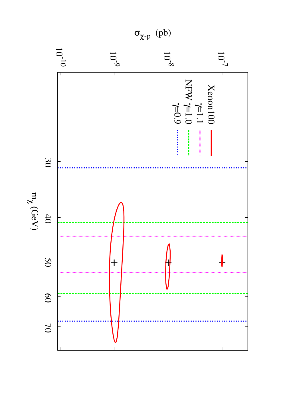
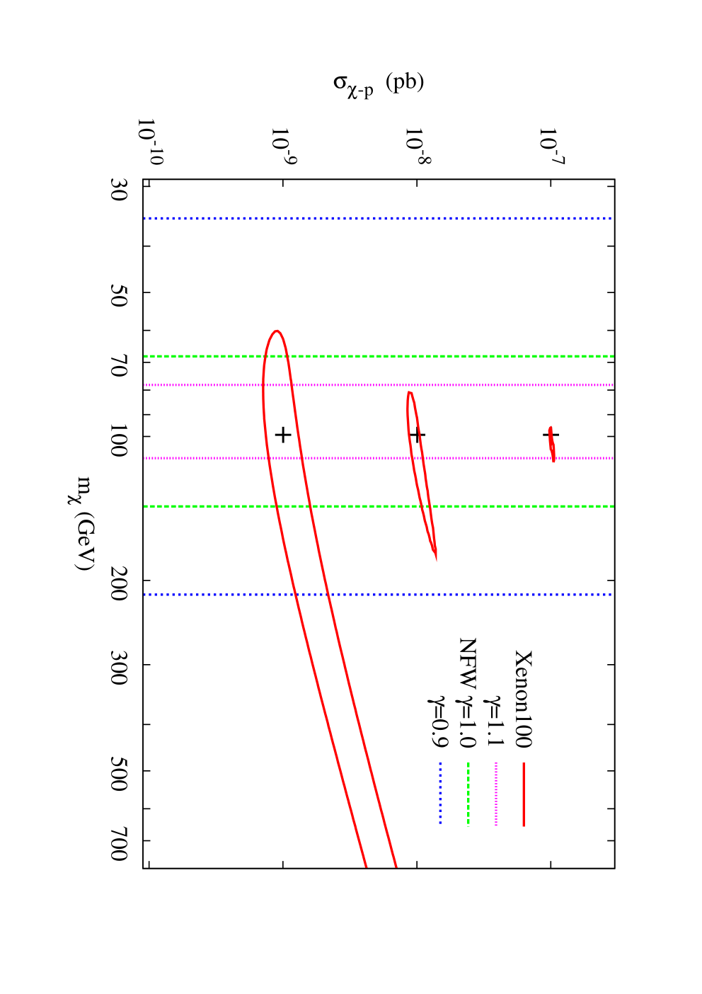
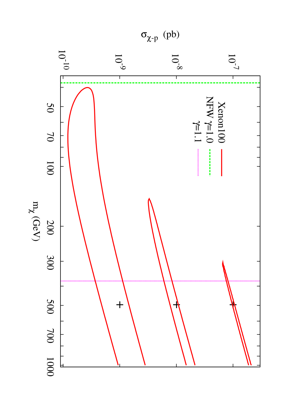
In Fig.2.13 we compare the precision level for both experiments as a function of the WIMP mass, for different values of the spin-independent cross-section ( $10^{-7}$ , $10^{-8}$ and $10^{-9}$ pb) and for different halo profiles. For this treatment we minimize the impact of uncertainties discussed in the previous paragraph, as we are mostly interested in examining the a priori, in some sense “intrinsic” sensitivity of the two detection techniques. For example, in the case of direct detection, the necessity for minimization of background noises and control of the noise sources has been repeatedly pointed out. As for uncertainties entering the velocity distribution of WIMPs in the solar neighborhood (or, why not, the form factor’s functional form), these can, in principle be minimized by measurements exterior to the experiments themselves. The same holds for most uncertainties in the case of indirect detection. As a small example, Fermi’s overall sky survey capacity is hoped to contribute in the minimization of uncertainties in non-DM annihilation sources, whereas other observations in different energy regions can also contribute in this direction. In this respect, for our comparative results, we remove the extra parameters from the statistical treatment. We see that at $95\%$ of confidence level Fermi, after $3$ years of exposure will have an equivalent sensitivity to the $100$ kg XENON experiment after $3$ years of running if $\sigma_{\chi-p}\lesssim 10^{-8}$ pb, independently of the WIMP mass. The indirect detection by Fermi will always be able to give an upper bound on the WIMP mass for $m_{\chi}\sim 100$ GeV, whereas the XENON $100$ kg experiment would only give a lower bound value if $\sigma_{\chi-p}\lesssim 10^{-9}$ pb. In all cases, the lower bounds given by Fermi for a NFW halo profile are similar to the ones given by the XENON $100$ kg experiment for any WIMP mass if $\sigma_{\chi-p}\lesssim 10^{-8}$ pb.

To compare the uncertainties on the WIMP mass expected from direct and indirect detection modes, we plotted in Fig.2.14 $\Delta m_{\chi}/m_{\chi}$ as a function of the WIMP mass for $\sigma_{\chi-p}=10^{-8}\mbox{pb}$ and a NFW halo profile. One can clearly see in the figure that Fermi will be competitive with XENON $100$ kg to measure the WIMP mass in the case of a NFW halo profile for $\sigma_{\chi-p}\lesssim 10^{-8}$ pb. For heavy WIMPs, Fermi could even be more sensitive than XENON.

2.4.5 WIMPs at present and future colliders

So far we have completely neglected colliders as a potential source of information on dark matter properties. However, there is a quite general agreement on the fact that despite the significant progress in astroparticle physics experiments, which manage to impose more and more constraints on various models, collider experiments remain an irreplaceable source of information for particle physics. It is quite natural thus, to examine the potential of colliders to constrain WIMP properties. We will examine the extent at which astroparticle and collider experiments become competitive, trying at the same time to stay as model-independent as possible.

This last point is, in fact, the major difficulty in treating collider experiments to extract astroparticle data: most studies performed for new physics at colliders are very strongly model dependent. This is almost unavoidable in the case of the LHC, due to the hadronic nature of the colliding particles. The fact that the initial energy of the colliding particles/partons is not well-known, since it is determined by the parton distribution functions, renders it extremely difficult (in fact, practically impossible) to look beyond the transverse plane. This obviously limits -up to a certain point- the precision that could be obtained with respect to, for example, an $e^{+}e^{-}$ collider. As a result, it is quite difficult to make predictions in a model-independent way, since a whole set of parameters must be taken into account in order to perform concrete predictions. The cruciallity of these uncertainties will become clearer in the following.

The Approach

Recently, an approach was proposed in references [146, 147] which allows to actually perform a model-independent study of WIMP properties at lepton colliders (such as the ILC project). The goal we pursue is to extract constraints which are as stringent as possible for a generic dark matter candidate. A generic WIMP can annihilate into pairs of standard model particles:

\chi+\chi\longrightarrow X_{i}+\bar{X}_{i}\ .

(2.38)

However, the procedure taking place in a collider is the opposite one, having only one species of particles in the initial state. The idea proposed in Ref. [146] is to correlate the two processes in some way. This can be done through the so-called “detailed balancing” equation, which reads:

\frac{\sigma(\chi+\chi\rightarrow X_{i}+\bar{X}_{i})}{\sigma(X_{i}+\bar{X}_{i}\rightarrow\chi+\chi)}=2\frac{v_{X}^{2}(2S_{X}+1)^{2}}{v_{\chi}^{2}(2S_{\chi}+1)^{2}}\ ,

(2.39)

where $v_{i}$ and $S_{i}$ are respectively the velocity and the spin of the particle $i$ . The cross-section $\sigma(\chi\chi\rightarrow X_{i}\bar{X}_{i})$ is only averaged over spins.

The total thermally averaged WIMP annihilation cross-section can be expanded as

\sigma_{i}v=\sum_{J=0}^{\infty}{\sigma_{i}^{(J)}v^{2J}}\ ,

(2.40)

where $J$ is the angular momentum of each annihilation wave. Now, for low velocities, the lowest-order non-vanishing term in the last equation will be dominant. So, we can express the total annihilation cross-section as a sum of the partial ones over all possible final states for the dominant partial wave $J_{0}$ in each final state:

\sigma_{an}=\sum_{i}{\sigma_{i}^{(J_{0})}}\ .

(2.41)

Next, we can define the “annihilation fraction” $\kappa_{i}$ into the standard model particle pair $X_{i}-\bar{X}_{i}$ :

\kappa_{i}=\frac{\sigma_{i}^{(J_{0})}}{\sigma_{an}}\ .

(2.42)

By combining Eqs. (2.39) and (2.42) we can obtain the following expression for the WIMP pair-production cross-section:

\sigma(X_{i}\bar{X}_{i}\rightarrow 2\chi)=2^{2(J_{0}-1)}\kappa_{i}\sigma_{an}\frac{(2S_{\chi}+1)^{2}}{(2S_{X}+1)^{2}}\left(1-\frac{4M_{\chi}^{2}}{s}\right)^{1/2+J_{0}}\ .

(2.43)

A few remarks should be made about the validity of this formula:

•

Equation (2.43) is valid for WIMP pair-production taking place at center-of-mass energies just above the pair-production threshold.
•

The detailed balancing equation is valid if and only if the process under consideration is characterized by time-reversal and parity invariance. It is well known that weak interactions violate both of them, up to some degree, which we ignore in this treatment.

A process of the form $X_{i}\bar{X}_{i}\longrightarrow\chi\chi$ is not visible in a collider, since WIMPs only manifest themselves as missing energy. At least one detectable particle is required for the event to pass the triggers. An additional photon from initial state radiation (ISR) is required to be recorded on tape: $X_{i}\bar{X}_{i}\longrightarrow\chi\chi\gamma$ . We can correlate the WIMP pair-production process to the radiative WIMP pair-production for photons which are either soft or collinear with respect to the colliding beams. In this case, the two processes are related through [146]:

\frac{d\sigma(e^{+}e^{-}\rightarrow 2\chi+\gamma)}{dxd\cos\theta}\approx{\cal{F}}(x,\cos\theta)\tilde{\sigma}(e^{+}e^{-}\rightarrow 2\chi)\ ,

(2.44)

where $x=2E_{\gamma}/\sqrt{s}$ , $\theta$ is the angle between the photon direction and the direction of the incoming electron beam, $\tilde{\sigma}$ is the WIMP pair-production cross-section produced at the reduced center of mass energy $\tilde{s}=(1-x)s$ , and $\cal{F}$ is defined as:

{\cal{F}}(x,\cos\theta)=\frac{\alpha}{\pi}\frac{1+(1-x)^{2}}{x}\frac{1}{\sin^{2}\theta}\ .

(2.45)

Now, by combining Eqs. (2.44) and (2.43) we get the master equation:

\frac{d\sigma}{dxd\cos\theta}(e^{+}e^{-}\rightarrow 2\chi+\gamma)\approx\frac{\alpha\kappa_{e}\sigma_{an}}{16\pi}\frac{1+(1-x)^{2}}{x}\frac{1}{\sin^{2}\theta}2^{2J_{0}}(2S_{\chi}+1)^{2}\left(1-\frac{4M_{\chi}^{2}}{(1-x)s}\right)^{1/2+J_{0}}\ .

(2.46)

It would be useful here to note that although the value of $\kappa_{e}$ is here arbitrary, this parameter acquires specific values in each model. As an example, in mSUGRA models $\kappa_{e}$ ranges roughly from $0.2$ to $0.3$ [146].

The problem now is that very collinear photons fall outside the reach of any detector, due to practical limitations in the coverage of the volume around the beam pipe. Also, typically, lower cuts are included in the detected transverse momentum of photons, $p_{T}=E_{\gamma}\sin\theta$ , in order to avoid excessive background signals at low energies. So, if we are to use this approach, we have to examine its validity outside the soft/collinear region. The accuracy of the collinear approximation for hard photons at all angles has been discussed in the original paper [146], with the conclusion that the approach works quite well.

However, an important point should be taken into account here. From the previous discussion on the validity of the method, we have to impose specific kinematic cuts on the detected photons. We consider the following conditions:

•

We demand an overall condition $\sin\theta\geq 0.1$ and $p_{T}\geq 7.5$ GeV in order to assure the detectability of the photons.
•

In order to assure the fact that any photon under examination corresponds to non-relativistic WIMPs, we demand $v_{\chi}^{2}\leq 1/2$ . This gives a lower kinematic cut, along with an upper cut corresponding just to the endpoint of the photon spectrum:

$\frac{\sqrt{s}}{2}\left(1-\frac{8M_{\chi}^{2}}{s}\right)\leq E_{\gamma}\leq\frac{\sqrt{s}}{2}\left(1-\frac{4M_{\chi}^{2}}{s}\right)\ .$ (2.47)

These conditions present a flaw: the energy limits depend on the mass we wish to constrain. On the other hand, for the reasons explained before, we cannot treat the signals without imposing such kinds of cuts, if we do not want either to misuse the method or stick to heavy WIMPs (which, for kinematic reasons, cannot be relativistic). The only way to evade this problem is to suppose that other dark matter detection experiments (or, eventually, the LHC in the framework of specific models) will have already provided us with some sort of limits on the WIMP mass. In this case, having an idea of the region in which the WIMP mass falls, we can also estimate the cuts that will safely keep us outside the relativistic region and only consider photons within this region.

The main source of background events is the standard model radiative neutrino production, $e^{+}e^{-}\longrightarrow\nu\bar{\nu}\gamma$ . Apart from these background events, various models predict additional signals of the form “ $\gamma$ + missing energy”, one of the most well-known examples being radiative sneutrino production [148, 149], predicted in the framework of several supersymmetric models. In the spirit of staying as model-independent as possible, we will ignore all possible beyond standard model processes.

Basic results for non-polarized beams

We place ourselves in the framework of the ILC project with a center-of-mass energy of $\sqrt{s}=500$ GeV and an integrated luminosity of $500$ fb^-1. In order to estimate the background events, we used the CalcHEP code [150, 151] to generate $1.242.500$ $e^{+}e^{-}\longrightarrow\nu\bar{\nu}\gamma$ events, corresponding to the aforementioned conditions. The total radiative neutrino production background can be seen in Fig.2.15. The peak at $E_{\gamma}=\sqrt{s}/2\cdot(1-M_{Z}^{2}/s)\simeq 241.7$ GeV corresponds to the radiative returns to the $Z$ resonance.

We generate a predicted “observable” spectrum for given values of the WIMP mass and the annihilation fraction. During this study, we do not proceed to a (more realistic) full detector simulation, as done for example in Ref. [152], but stick to prediction levels in order to perform as thorough a scan as possible in the $(m_{\chi},\kappa_{e})$ parameter space and to have a picture of the “a priori” potential of the method.

Figure 2.16 shows the predicted ability of the ILC to determine WIMP masses and annihilation fractions for four points in the $(m_{\chi},\kappa_{e})$ parameter space for a $68\%$ and $95\%$ Confidence Level. These results concern WIMPs with spin $S_{\chi}=1/2$ and an angular momentum $J_{0}=1$ which corresponds to an annihilation cross-section $\sigma_{an}=7$ pb [146]. As can be seen, we are able to constrain quite significantly the WIMP mass ( $20\%-40\%$ precision), while constraints on $\kappa_{e}$ are weaker.

Figure 2.17 shows the relative error ( $\Delta m_{\chi}/m_{\chi}$ ) for the mass reconstruction as a function of $m_{\chi}$ , for $\kappa_{e}=0.3$ and a $95\%$ confidence level. The solid line corresponds to the proper treatment including kinematic cuts. For indicative reasons, we also show the abused results obtained if we do not impose kinematic cuts on the photon energy (dashed line). The amelioration of the method’s efficiency is obvious, although this is after all a false fact, since we include regions in which the approach is not valid. Above $m_{\chi}\simeq 175$ GeV the two lines become identical, since the WIMPs cannot be relativistic. The capacity of the method peaks significantly for masses of the order of $175$ GeV because around this value we reach an optimal combination of phase space volume and available spectrum that passes the kinematic cuts. As we move away from this value the accuracy tends to fall.

Let us make a final remark on the possibility of adopting a similar approach in the case of the LHC. As we argued before, the large uncertainty in the collision energy affects significantly the precision of the whole procedure (which is, already, based on approximations). Formally, in order to perform such a study for the LHC, the computed cross-sections must be convoluted with the proton parton distribution functions. As an additional element, the photon background in the LHC is expected to be much greater than in the ILC. The possibility of determining WIMP properties through a model-independent method at the LHC has been addressed to in Ref. [153], where the authors conclude that WIMP detection will be extremely difficult, if even possible.

Polarized beams

The reach of the ILC can be further increased by polarizing the beams. For polarized beams, the signal cannot be fully characterized by $\kappa_{e}$ ; instead, four independent annihilation fractions are needed, corresponding to the four possible $e^{+}e^{-}$ helicity configurations.

To apply Eq. (2.46) to this case, we make the replacement:

	$\displaystyle\kappa_{e}$	$\displaystyle\rightarrow$	$\displaystyle\frac{1}{4}(1+P_{-})\,\left[(1+P_{+})\,\kappa(e_{-}^{R}e_{+}^{L})+(1-P_{+})\,\kappa(e_{-}^{R}e_{+}^{R})\right]$		(2.48)
		$\displaystyle+$	$\displaystyle\frac{1}{4}(1-P_{-})\,\left[(1+P_{+})\,\kappa(e_{-}^{L}e_{+}^{L})+(1-P_{+})\,\kappa(e_{-}^{L}e_{+}^{R})\right]\ ,$		(2.48)

where $P_{\pm}$ are the polarizations of the positron and the electron beams. As in ref [146, 152], let us assume that the WIMP couplings to electrons conserve both helicity and parity: $\kappa(e_{-}^{R}e_{+}^{L})=\kappa(e_{-}^{L}e_{+}^{R})=2\,\kappa_{e}$ and $\kappa(e_{-}^{R}e_{+}^{R})=\kappa(e_{-}^{L}e_{+}^{L})=0$ .

In Fig.2.18 we show the relative error for the mass reconstruction for $\kappa_{e}=0.3$ and $95\%$ confidence level, for the unpolarized scenario and for two different polarizations: $(P_{-},P_{+})=(0.8,0)$ and $(0.8,0.6)$ .

2.4.6 Complementarity and Conclusions

In Fig.2.19 we compare the precision levels for direct and indirect detection experiments, along with the corresponding results of the method we followed for the ILC for two cases of WIMPs masses, $m_{\chi}=100$ GeV and $175$ GeV, and $\kappa_{e}=0.3$ . We plot the results in the $(m_{\chi},\kappa_{e})$ plane. This is done as the $\kappa_{e}$ parameter entering the ILC treatment presented before is, in fact, the same parameter as the corresponding branching ratio $Br_{i}=\frac{\langle\sigma_{i}v\rangle}{\langle\sigma v\rangle}$ appearing in Eq. (2.14) for $i=e$ .

The blue-dotted line corresponds to a $100$ kg XENON experiment, where the WIMP-nucleus cross-section has been assumed to be $10^{-8}$ pb. The green-dashed line depicts the results for a Fermi-like experiment assuming a NFW halo profile. The total annihilation cross-section into standard model particles has been taken to be $\langle\sigma v\rangle=3\cdot 10^{-26}$ cm³s^-1. The red-plain line represents our results for an ILC-like collider, with non-polarized beams. All the results are plotted for a $95\%$ confidence level.

We can see that for different regions of the WIMP mass, the three kinds of experiments that we have used as prototypes can act in a highly complementary way. For example, in the case of a 100 GeV WIMP, indirect detection or an ILC-like experiment alone can provide us with limited precision both for the WIMP mass (of the order of $60\%$ ) and the $\kappa_{e}$ parameter (where the results are even worse). Combined measurements can dramatically increase the precision, reaching an accuracy of $25\%$ in mass. If we additionally include direct detection measurements, we can further increase the precision.

In the case of a $175$ GeV WIMP, a point where the unpolarized ILC sensitivity peaks, we see that the dominant information comes from this source. Nevertheless, even if we only combine direct and indirect detection experiments, we see that we can, in fact, acquire non-negligible constraints on the dark matter candidate mass.

$m_{\chi}$	XENON	Fermi	ILC
$50$ GeV	$-5/+7$ GeV	$\pm 12$ GeV	$-$
$100$ GeV	$-19/+75$ GeV	$-50/+60$ GeV	$-40/+20$ GeV
$175$ GeV	$-65/$ GeV	$-125$ GeV	$-20/+15$ GeV
$500$ GeV	$-$	$-$	$-$

Table 2.4: Precision on a WIMP mass expected from the different experiments at a

95\%

CL after 3 years of exposure,

\sigma_{\chi-p}=10^{-8}

pb a NFW profile and a 500 GeV unpolarized linear collider with an integrated luminosity of 500

\mbox{fb}^{-1}

To summarize the analysis, we show in Table 2.4 the precision expected for several interesting dark matter masses. Whereas a light WIMP (50 GeV) can be reached by both types of dark matter experiments with a relatively high level of precision, our analysis fails in the ILC case because of the relativistic nature of the WIMP. On the contrary, the ILC would be particularly efficient to discover and measure a WIMP with a mass of about 175 GeV. Concerning a 500 GeV WIMP, which is kinematically unreachable at the linear collider, it would be difficult to be observed by Fermi or XENON. Only a lower bound could be determined experimentally.

We have discussed the possibility of identifying WIMP properties in a model-independent way. For that we have considered direct and indirect searches, and in particular the interesting cases of a XENON $100$ kg experiment and the Fermi satellite. We have shown that whereas direct detection experiments will probe efficiently light WIMPs given a positive detection (at the $10\%$ level for $m_{\chi}\lesssim 50$ GeV), Fermi will be able to confirm and even increase the precision in the case of NFW profile, for a WIMP-nucleon cross-section $\sigma_{\chi-p}\lesssim 10^{-8}$ pb.

Moreover, both XENON and Fermi are in principle complementary with a future ILC project, and the measurements from the three experiments will be able to increase significantly the precision that we can reach on the mass of the WIMP.

In this chapter we introduced the basic formalism we shall be using in the following in order to compute event rates and examine the detectability of various dark matter candidates in a series of experiments. We also presented an (somehow outdated we should say) analysis of the capacity of three major detection modes to constrain dark matter properties. But, so far, we have said very few on specific models that try to explain dark matter. This will be the topic of the following chapters.

Chapter 3 A minimal solution to the Dark Matter problem

In the first chapter we explained why the Standard Model is unable to answer the Dark Matter question. In short, it does not contain any electrically and color neutral particle that can be produced non-relativistically. Therefore, if one wishes to try and explain the dark matter problem, it is unavoidable to look for candidates in extensions of the Standard Model of particle physics. In this chapter, we describe one of the simplest such extensions that have been proposed in the literature, the singlet scalar model of dark matter.

3.1 Some introductory remarks

There is a plethora of theories beyond the standard model. They are often motivated by some experimental discrepancy with respect to the theory (dark matter, neutrino masses, LEP-2 excess). In other cases, they try to resolve some problems appearing in the standard model itself from a theoretical (someone could say almost aesthetic) point of view. Finally, some extensions are even manifestly motivated by curiosity.

Although a full listing is quite difficult, we could cover a large variety of these extensions by categorizing them within three or four large classes:

•

One can extend the particle content and/or the gauge group. A simple example in this direction will be described in the present chapter.
•

One can add spacetime dimensions which usually amount to new particles and interactions in the four-dimensional spacetime. These theories, usually called extra-dimensional ones shall not be dealt with in this work, despite their significant interest. Some notable references in this class of models are [154, 155, 156, 157, 145, 158, 159].
•

Finally, one can think of extending the Poincaré symmetry characterizing current quantum field theories. This is the example of supersymmetry, that we shall examine in the next chapter.

It is interesting to note, as an introductory remark, that several among these approaches (actually, all of them!) were not initially introduced in relation to the dark matter issue. The fact that they can actually provide us with viable candidates is often an unexpected as well as impressive fact.

So far, we have implicitly made an assumption which obviously imposes a huge restriction to the potential number of models that could solve the dark matter problem: that dark matter actually consists of a single particle. This is a very common simplification. Although multi-candidate models do exist, most approaches are interested in finding exactly one candidate in each model. A first reason is that obviously it is easier to deal with a single particle rather than a certain number of them. Secondly, our description of the so-called “WIMP miracle” presents us with an intriguing possibility: solving the Boltzmann equation for a single particle can, indeed, amount quite naturally to searching for candidates in an -in principle- experimentally reachable energy scale which can account for the entire quantity of dark matter in our universe. Were we to suppose a large number of components, we would practically have all the freedom in the world to introduce as many candidates as we want with couplings and masses in essentially all energy scales. Finally, we should say (and this shall be explicited in the following) that as it turns out, finding a stable or quasi-stable particle in a model is not that easy a task, especially if we wish to couple it to some Standard Model sector in a non-purely gravitational manner. For example, if we were to consider a candidate coupled to two lighter fermions, the candidate could easily decay, spoiling the picture of thermal relics. The stability or quasi-stability of a dark matter candidate is practically always imposed by some discrete symmetry, rendering the lightest BSM particle (i.e. exactly one) stable.

In the following, hence, we shall see that within all models we examine there is one and only one dark matter candidate which should account for the entire amount of dark matter in our universe. This has important repercussions, since in the case of multi-component dark matter, each individual component need only respect the upper WMAP bound. On the contrary, in the case of single-component dark matter, both the upper and the lower bound must be taken into account. So, the self-annihilation cross-section of the candidate is not only bound from below but also from above.

3.2 The singlet scalar extension of the Standard Model

Among the three possibilities for extensions to the standard model we presented previously, the first is perhaps the most straightforward one. If we leave the SM gauge group intact, we can add some more particle fields to the already existing particle content transforming according to our desired representations of $SU(3)_{C}\times SU(2)_{L}\times U(1)_{Y}$ and examine if they can constitute viable dark matter candidates. Evidently, describing the process as such is an enormous oversimplification, since a whole number of experimental or theoretical constraints should be respected. We shall see such examples in the paragraphs to follow.

Perhaps the simplest choice that can be made is the addition of a scalar field, being completely neutral under the entire gauge group, but acquiring part of its mass through the usual Higgs mechanism. The field is hence only coupled to the Standard Model through its interaction with the Higgs field. Although such a model had previously been considered in the literature, it was first introduced as a potential solution to the dark matter problem in $1994$ [160]. If we stick to the case of a single scalar singlet (in the original paper the possibility for a larger number is also considered) coupled to the standard model only through the Higgs sector, the most general renormalizable tree-level Lagrangian that can be written is

{\cal{L}}={\cal{L}}_{SM}+{\cal{L}}_{S}

(3.1)

where ${\cal{L}}_{SM}$ is the usual standard model Lagrangian and ${\cal{L}}_{S}$ is the Lagrangian involving the singlet field $S$ :

{\cal{L}}_{S}=\frac{1}{2}\partial_{\mu}S\partial^{\mu}S-\frac{1}{2}m_{0}^{2}S^{2}-\lambda_{1}SH^{\dagger}H-\lambda S^{2}H^{\dagger}H-\frac{\lambda_{3}}{3}S^{3}-\frac{\lambda_{S}}{4}S^{4}

(3.2)

where for the moment, $S$ can be a complex field. In its present form, this Lagrangian does not guarantee the stability of $S$ : if for example the scalar were to be heavier than twice the Higgs boson mass, it could easily decay into a Higgs pair due to the term $\sim SH^{\dagger}H$ that induces a singlet-Higgs-Higgs vertex. To assure stability, we further impose a $Z_{2}$ symmetry (i.e. $S\rightarrow-S$ ) under which the singlet is odd whereas all other particles are even. Referring to Eq.(3.2), doing so eliminates the terms proportional to $\lambda_{3}$ and $\lambda_{1}$ . Furthermore, we make a simplifying assumption, that the $S$ field is real. We note that a linear term is forbidden by the $Z_{2}$ symmetry, but would be permitted in the original Lagrangian. Even if the $Z_{2}$ symmetry were absent though, such a term could be eliminated by a redefinition of the vacuum energy.

The previous assumptions amount to a Lagrangian

{\cal{L}}_{S}=\frac{1}{2}\partial_{\mu}S\partial^{\mu}S-\frac{m_{0}^{2}}{2}S^{2}-\frac{\lambda_{S}}{4}S^{4}-\lambda S^{2}H^{\dagger}H

(3.3)

The model introduces, hence, three new parameters: the scalar mass $m_{0}$ , the scalar’s self-coupling $\lambda_{S}$ and the quartic coupling of the scalar to the Higgs field $\lambda$ . The first two are parameters “internal” to the pure $S$ sector. The third one determines the coupling strength of $S$ to the visible sector, through its interaction with the Higgs. We note that since $\lambda_{S}$ does by no means affect the visible sector, it is difficult to directly constrain its value.

When the Higgs field acquires a non-zero vacuum expectation value, the scalar mass receives contributions from terms of the form $\lambda v^{2}S^{2}$ which shifts the actual tree-level mass to

m_{S}^{2}=m_{0}^{2}+\lambda v^{2}\ ,\ \

(3.4)

from which we can clearly see that we can change the free parameter basis from $(m_{0},\lambda,\lambda_{S})$ to $(m_{S},\lambda,\lambda_{S})$ . At tree-level, the $\lambda_{S}$ parameter does not contribute to dark matter phenomenology and is therefore an irrelevant parameter for most dark matter - related analyses. Taking into account the fact that the Higgs boson has not yet been discovered, there are thus three free parameters of interest overall, namely $(m_{S},\lambda,m_{h})$ with the latter being the Higgs mass, which is nevertheless bound by LEP and LEP-2 measurements, as well as theoretical constraints, having a minimal allowed value of $114.4$ GeV. If we further demand that at the true vacuum of the theory $<S>=0$ , we can avoid mixing effects between the scalar and the Higgs boson. The singlet’s mass has a priori no reason to lie in the electroweak scale: in fact, being a scalar that is not protected by some symmetry (as is the case of gauge symmetry for gauge bosons and chiral symmetry for fermions), its mass receives loop contributions depending quadratically on the theory’s cutoff scale $\Lambda$ which can push the mass up to the Planck scale. However, for naturalness reasons, it is reasonable to expect that $m_{S}$ should fall roughly withing the electroweak scale.

Despite its simplicity, it turns out that this simple extension of the Standard Model can provide an interesting phenomenology and has been examined in the literature to quite some extent. Before going on to discuss various constraints and phenomenological issues related to the model, we just note that even more interesting effects can be introduced if one departures from the singlet scalar case and introduces, for example, a scalar doublet [161, 162, 163, 164, 165, 166, 167, 168, 169, 170, 171, 172, 173, 174, 175] or a fermion multiplet [176, 177, 178, 179, 180] . But this is probably the truly simplest extension imaginable within the framework of renormalizable four - dimensional theories.

3.3 Constraints and collider phenomenology

Although this might seem as a rather simplistic approach, we can divide the constraints on the model into two main categories, theoretical and experimental. Theoretical constraints can come from requirements such as vacuum stability, perturbativity, unitarity and so on. Experimental constraints can come mainly from precision electroweak measurements and direct searches at lepton colliders, or the requirement that the model reproduces the correct dark matter relic density.

3.3.1 Theoretical constraints

Three types of theoretical constraints have been so far discussed in the literature: unitarity, perturbativity and stability of the EWSB vacuum. In all cases, the authors stick to the case of a real scalar field.

Perturbative unitarity constraints have been examined in [181]. Unfortunately, the authors conclude that their analysis does not restrict the scalar mass $m_{S}$ . The main bounds that can be obtained is that the Higgs mechanism contribution to the scalar mass cannot be larger than $900$ GeV and that for $m_{h}\in(114.5,251)$ GeV and $\lambda\in(0.21,0.97)$ GeV the model parameters must satisfy the relation

6\lambda_{S}+\frac{4\lambda^{2}}{8\pi}\lesssim 8\pi\ .\ \

(3.5)

Vacuum stability and perturbativity constraints in their turn have been studied in detail in [182]. In this paper, the authors perform an analysis of the one-loop effective potential and find that not only one can extract limits on the dark matter - related quantities, but interesting bounds can even be found on the value of the scalar self-coupling especially when the relic density constraint is taken into account in combination with others. The effective potential at $1$ -loop order is calculated and its scale invariance imposes the introduction of running parameters for the couplings and masses as usually in renormalization procedures. Due to the structure of the model, the addition of the scalar does not contribute to the RGE evolution of the usual SM parameters other than those that enter the scalar potential, which can be written in its turn as

V_{eff}(h,S)=V_{tree}(h,S)+V_{1-loop}(h,S)

(3.6)

where the tree-level and 1-loop pieces of the scalar potential are, in our notations,

V_{tree}(h,S)=\mu^{2}H^{\dagger}H+\lambda_{h}(H^{\dagger}H)^{2}+\frac{m_{0}^{2}}{2}S^{2}-\frac{\lambda_{S}}{4}S^{4}-\lambda S^{2}H^{\dagger}H

(3.7)

and

V_{1-loop}(h,S)=\sum_{j}\frac{n_{j}}{64\pi^{2}}m_{j}^{4}(h,S)\left[\log\left(\frac{m_{j}^{2}(h,S)}{\mu_{r}^{2}}\right)-c_{j}\right]

(3.8)

where $h,S$ denote the classical fields defined as functional derivatives with respect to external sources of the generating functional that only generates connected Green’s functions and $\mu_{r}$ is the renormalization scale. We should note a slight change in notation with respect to the first chapter, where the initial Higgs doublet was denoted as $\Phi$ and the quartic Higgs coupling as $\lambda$ , a symbol which at this point we reserve for the $S$ scalar quartic coupling, denoting the corresponding Higgs coupling as $\lambda_{h}$ .

Scale invariance of (3.6) and previous knowledge of the standard model $\beta$ and $\gamma$ functions for the unaffected parameters allow the authors to fully determine the beta functions for all parameters of the model (imposing, of course, appropriate boundary conditions).

Then, the conditions the authors demand are that no remote vacuum be formed below the cutoff $\Lambda$ of the theory, to assure vacuum stability, as well as that no Landau pole appears below the cutoff in order to ensure perturbativity. Many more details as well as explicit formulae can be of course found in the original paper.

Of particular interest for our work are the results obtained under the condition that the WMAP constraints be satisfied in a saturated manner. Assuming a Higgs mass of $120$ GeV, the bounds on $(m_{S},\lambda)$ combinations depend strongly on one hand on the value of the scalar self-coupling (the bounds being alleviated as the coupling increases) and on the other hand on the scale at which we consider that new physics enter the game. For self-coupling of ${\cal{O}}(1)$ , the model is practically unconstrained, especially if the cutoff is placed near the EW scale.

3.3.2 Some notes on collider phenomenology

In the general case where a real singlet scalar field is added to the Standard Model, it can mix with the usual Higgs boson and affect not only the phenomenology of the latter, but also a whole series of electroweak observables. This analysis has been performed in detail by Barger et al in [183]. More specifically, the mixing is expected to bring about important changes in the gauge boson propagator functions involved in several processes and quantities such as the $W$ mass, atomic parity violation or $Z$ - pole observables.

In our case, however, we already mentioned that for the scalar to be completely stable, we impose a discrete symmetry to the Lagrangian. This eliminates all mixing effects with the Standard Model Higgs. In this case, practically all experimental constraints are completely alleviated, at least from the point of view of collider physics. Nevertheless, even in this case it is possible to have interesting effects especially on Higgs discovery physics at the Large Hadron Collider or the ILC.

If the Singlet is light enough so that $m_{h}>2m_{S}$ , the Higgs boson decay modes can be significantly modified, since the possibility for invisible decays into a singlet pair is open. In this case, as explained in the same paper, one should expect (depending on the singlet mass as well as on the strength of the singlet-singlet-Higgs coupling) significant modifications on the Higgs discovery potential of the LHC. More specifically, and especially in the Light Higgs scenario, fermionic decay modes can by dominated by the invisible decays. Whereas the Higgs boson discovery potential thus deteriorates in the other channels, there can be discovery in the invisible channel through observation of events with missing energy in Vector Boson Fusion or Higgstrahlung processes. Furthermore, modifications can be sizeable in the Higgs total decay width.

Interestingly, it turns out that low-mass singlets can further severely alter expectations on $b\rightarrow s$ transitions in the decays of $B$ mesons to Kaons along with missing energy [184]. These effects could be measurable in $b$ - factories and could constrain the very low mass regime of the model, for $m_{s}<2$ GeV. Current data can already put bounds for lower masses, excluding a significant portion of that region of the parameter space.

The major constraints in the $Z_{2}\times$ SM case come from imposing dark-matter related limits, especially the demand to reproduce the observed relic density as well as the imposition of bounds coming from direct detection experiments.

3.3.3 Relic density

The relic density constraint has been examined in a series of papers [160, 182, 183, 185, 186, 187] for different regions of the model’s parameter space and at times under different assumptions concerning the singlet itself (especially concerning its real or complex nature), depending also on the emphasis that each author wishes to give on specific aspects of the model’s phenomenology. The relic abundance calculation is actually really simple compared to more extended models with several possible annihilation channels. The singlet coupling only to the Higgs sector, the only diagram entering the calculation of $<\sigma v>$ is the $s$ - channel exchange of a Higgs boson between a pair of singlets and the final state particles. The dark matter constraint can be satisfied in significant portions of the parameter space $(\lambda,m_{s},m_{h})$ . The $\lambda_{S}$ parameter, as we already mentioned, is irrelevant for the calculations and might only enter indirectly through the constraints described in the previous sections. An instructive way to represent the parameter combinations that satisfy the constraint can be found for example in [187]. We borrow fig.3.1 from this paper in order to explain the general parameter space behavior.

In this figure, the author plots the WMAP-compliant regions in the $(m_{s},\lambda)$ plane for various values of the Higgs mass, represented in fig.3.1 as lines or regions of different colors. In practice, the author scans the model’s parameter space in order to find points that satisfy the constraint $\Omega_{S}h^{2}=0.11$ . For the case $m_{h}=120$ GeV, the entire region compatible with the $2\sigma$ region allowed by WMAP is plotted. It is particularly noteworthy that, as mentioned in the paper, for reasonable values of $\lambda$ the model can account for the DM relic abundance by keeping the singlet’s mass near the electroweak scale, so the corresponding DM candidate is a characteristic illustration of WIMP dark matter.

The most striking feature upon imposition of the WMAP limits is the steep decline in the required $\lambda$ value for specific values of the scalar mass, varying according to the Higgs boson mass. The first of these regions corresponds to the case where $m_{s}\approx{\cal{O}}(m_{h}/2)$ , where annihilation is done through a practically on-shell Higgs propagator. In this case, the squared propagator entering the relevant amplitude explodes in value providing an enormous boost to the annihilation cross-section, hence the WMAP data can be satisfied only by significantly decreasing the value of the relevant coupling. Seen inversely, by keeping $\lambda$ constant, once the $h$ -pole is reached the relic density falls dramatically and $S$ can no longer account for the observed relic abundance. The enhancement of $\sigma v$ depends of course on the total width of the Higgs. This is the reason why as the Higgs mass increases, so does the required $\lambda$ value in order to satisfy WMAP. For the same reason, the increase in the Higgs width, the resonance area tends to become less narrow for larger Higgs masses.

The second feature concerns the fall in the required $\lambda$ values in order to reproduce the DM relic density for moderate Higgs masses and slightly above the Higgs resonance. This feature stays practically constant with changes in $m_{h}$ . It corresponds to the $W^{+}W^{-}$ pair-production threshold, where $m_{h}\sim m_{W}$ . Once again the cross-section increases and the required singlet-singlet-Higgs coupling must be smaller so as not to underpoduce dark matter. This feature is more striking for lower Higgs masses, whereas as $m_{h}$ increases the two resonances overlap.

A further feature is that for smaller singlet masses, the required $\lambda$ values in order to reproduce the DM relic density are comparably higher than for higher ones. Once again, this is a mainly kinematic effect. Since the cross-section rises as the incident particle mass approaches the outgoing ones, once the gauge boson channels open the singlet tends to annihilate mostly into $W^{+}W^{-}$ and $ZZ$ pairs, which are evidently closer in mass than quarks or leptons. Furthermore, we see that as $m_{S}$ grows further beyond the $W$ -resonance, the corresponding $\lambda$ values tend to increase once more.

The resonance regions let aside, for $m_{h}$ values of roughly $120$ - $200$ GeV, we see that the coupling values in order to get the correct relic density are of the order of $10^{-1}$ for small masses and around $10^{-2}$ for masses up to $300$ GeV. These are the regions which are the most relevant for indirect detection, as we shall see in the following.

Direct detection constraints have also been examined by a number of authors and under different points of view [183, 185, 187, 188, 93, 186]. In most cases, the authors use existing data in order to impose bounds on the model parameters. After the excesses reported by DAMA but also CDMS-II and CoGeNT, there have been efforts to examine whether the singlet scalar model can account for these excesses. The nature as well as the uncertainties entering some of the latest reported excesses are still under discussion, but at first approach the model seems to be able to reconcile them. Furthermore, as discussed in [93] near-future measurements will be able to give a definitive answer on the point. In a recent review [189] the model is confronted with the latest constraints coming from CDMS-II and XENON. It turns out that if standard assumptions are made, and for a Higgs mass of $120$ GeV, the CDMS-II results alone exclude singlet masses roughly up to $80$ GeV. If the XENON-100 results are also taken into account, practically the entire parameter space for masses up to $200$ GeV are excluded. The only region evading detection is the $h$ -pole one, since the required $\lambda$ value is, as we explained, much smaller. We note that this region falls largely outside the reach of all planned direct detection experiments.

3.4 Gamma-rays detection prospects

Apart from its interesting relic density, direct detection and collider phenomenology, the singlet scalar model of dark matter has implications for indirect detection experiments as well. This has been studied in [187] for the case of gamma-rays coming from DM annihilations (excluding the Galactic Center) and in [190] for positrons and antiprotons. We note that in [189] the results of the second of these papers are summarized and extended as far as the considered Higgs mass is concerned.

Let us first summarize the results concerning gamma-rays. For instructive reasons, once again, we give in fig.3.2 the plot from ref.[187] summarizing the author’s findings.

In this figure, the blue lines follow the model’s viable parameter space, where the singlet mass is varied and the value of $\lambda$ is fixed for every mass by imposing the relic density constraint. We remind that, and this also concerns the following antimatter treatment we shall present, the dark matter relic density is fixed to its central value (in the case of this paper this is $\Omega_{DM}h^{2}=0.11$ ) and not varied in the whole WMAP-allowed region. The effect of allowing for such a variation would just result to the lines being transformed to narrow regions around this central value. In this respect, the results are representative. Then, the corresponding values of $<\sigma v>_{v\rightarrow 0}$ are calculated, which are relevant for indirect detection at present times when the WIMP velocity is small. The considered profile is the standard Navarro, Frenk and White one, although since the GC is excluded from the analysis this is not such and important factor.

The observed behavior is very smooth: $<\sigma v>_{v\rightarrow 0}$ remains practically constant for all singlet masses. Then, two important features appear. The first one is situated at the point where $2m_{S}\sim m_{h}$ , where we have resonant annihilation into a Higgs propagator. The second one appears for the case of on-shell production of a pair of $W$ vector bosons. Why does this fluctuation appear? The answer lies in the fact that $<\sigma v>$ and $<\sigma v>_{v\rightarrow 0}$ are calculated for different kinematic regimes. In order to obtain the correct relic density, and for typical Weakly Interacting Massive Particles as in our case, a - more or less - standard value of the total thermally averaged self-annihilation cross-section is needed. We already saw that in these two regions, this value is obtained through a combination of low $\lambda$ values and the fact that annihilation takes place resonantly. The $\lambda$ value stays practically the same at present times. The resonance conditions, however, do not. Since during decoupling WIMPs have a non-negligible velocity, the resonance occurs slightly lower than the points where $2m_{S}=m_{h}$ or $m_{S}=m_{W}$ . What actually matters is the total energy of the singlets at that time and not just the one associated to their mass. Hence, for the specific points, the correct relic density was obtained for small $\lambda$ values but for resonance conditions which are no longer valid.

To corroborate these comments, we should notice the rise in $<\sigma v>_{v\rightarrow 0}$ right after the Higgs resonance. Being at the zero velocity limit, a small rise in the WIMP mass can reproduce resonant annihilation which compensates the smallness of the scalar-scalar-Higgs coupling as soon as we are practically exactly at $m_{S}=1/2m_{h}$ . This is manifest in the cases of $m_{h}=120,180$ and $200$ GeV but not in the $m_{h}=150$ GeV one. The most plausible explanation for this is that since the two resonance regions get very close, the peak that would appear after the $h$ resonance is immediately killed by the fall in $\lambda$ due to the $W^{+}W^{-}$ one.

Now, as expected, the Fermi detection limits do not present any particular features. For the same mass values the limits do obviously not depend on the model parameters as such. Small variations from one Higgs mass scenario to another are the result of small differences in the final state composition, which in any case is mostly $b\bar{b}$ below the W resonance and $W^{+}W^{-}$ above. So, the detectability lines are practically the same among the different cases. We see that for masses up to roughly $180$ GeV the perspectives are really good for both background models, whereas heavier singlets are visible for the “conventional” background only, which is lower than the “optimized” one.

3.5 Antimatter Detection

In ref.[190] we studied the corresponding prospects for antimatter (positron and antiproton) detection at the AMS-02 mission as well as the constraints coming from the existing PAMELA collaboration data. We used the public code micrOMEGAs, which in its latest versions gives the possibility to compute the relic density for WIMP-type candidates in generic models in order to define the viable parameter space. We examined singlets with masses lying in the region $50\leq m_{S}\leq 600$ GeV fixing the Higgs mass at $m_{h}=120$ GeV, then varying $\lambda$ so as to get a relic density of $\Omega_{DM}h^{2}=0.11$ .

In fig.3.3 we show the Branching Fractions (BRs) at zero velocity for our mass range and for the points satisfying the relic density constraint.

We see the behavior described in the previous, namely that for small masses the final state is dominated by the $b\bar{b}$ component, whereas above the $W$ threshold the most important channel is the $W^{+}W^{-}$ one. Smaller - but existing - contributions come from $hh,ZZ,c\bar{c}$ and $t\bar{t}$ final states. At this point, it should be noted that a novel estimation of the final state composition and the self-annihilation cross-section in [191] demonstrates that in the low-mass regime, $3$ - body final state contributions can also be sizeable.

3.5.1 Antiproton detection

Our first study concerns the constraints coming from the PAMELA experiment and the detection perspectives with AMS-02 in the antiproton channel. We compute our results for the three propagation models MIN, MED and MAX as defined in the previous chapter assuming a smooth dark matter halo, as well as taking into account potential substructure enhancing the annihilation rate.

In order to assess the background, we repeat that the relatively recent PAMELA data are well reproduced by the conventional propagation model of Strong and Moskalenko. We thus consider that the experiment’s results are essentially comprised of background events and just fit their spectrum, taking care so as to maintain a good normalization to the low-energy data.

In this treatment, we shall characterize a point as being “3- $\sigma$ excluded” if the sum of the signal produced by this point and the background events surpass the PAMELA measurements by more than $3$ standard deviations, as stated by the collaboration itself. On the other hand, in order to assess a point as being detectable by AMS-02 we employ a $\chi^{2}$ criterion. The $\chi^{2}$ is defined as

\chi^{2}=\sum_{n=0}^{N}\frac{(\phi^{tot}_{n}-\phi^{bkg}_{n})^{2}}{(\phi^{tot}_{n})}A\cdot T\ ,

(3.9)

where $\phi^{tot}$ is the total antiproton flux, $\phi^{bkg}$ is the background flux, $N$ is the number of energy bins considered, $A$ is the geometrical acceptance of the experiment, and $T$ is the data acquisition time. It is reminded that AMS-02 is expected to take data for three years and features an antiproton geometrical acceptance of $330$ cm²sr [132]. We consider $20$ energy bins evenly distributed in logarithmic scale between $10$ and $300$ GeV. A $95\%$ confidence level corresponds then to $\chi^{2}>31$ .

We present our results in the same way as done in [187] for gamma-rays. To obtain the excluded regions in the plane ( $m_{S},<\sigma v>$ ), we first compute, for a model with the same branching ratios as the singlet scalar model (see figure 3.3), the value of $<\sigma v>$ required to exclude the model, $<\sigma v>_{excl}$ . By comparing $<\sigma v>_{singlet}$ with $<\sigma v>_{excl}$ we can then determine whether the model is excluded or not at a given singlet mass and according to our exclusion criterion. An analogous procedure is followed to determine the detectable regions.

In fig.3.4 we start the presentation of our results by comparing the minimal cross-sections that would be required for each mass value and for the three propagation models against the relevant singlet scalar’s model predicted cross-sections in order to satisfy the relic density constraint.

In the figure, the red/dashed, green/dotted and blue/dotted-dashed curves concern the MIN, MED and MAX models respectively, whereas the black solid line the model’s prediction. We immediately see that no parameter space point is yet excluded for any of the three propagation models. However, we observe that the small region corresponding to the point where two singlets annihilate resonantly into a Higgs propagator is at the verge of exclusion for the MAX model.

Then, in fig.3.5 we plot the corresponding minimal cross-sections that would be needed in order to have a positive detection in AMS-02.

We see that the model has really good perspectives for antiproton detection. Some portion of its parameter space will be probed for all three propagation models, whereas for the MED and the MAX one practically the entire viable parameter space will be visible, apart from the points corresponding to the $h$ -resonance during decoupling as well as the corresponding $W^{+}W^{-}$ resonance.

The next step is to consider possible effects of substructure in the galactic halo. In fig.3.6 we plot the exclusion limits for the three propagation models as denoted in each plot’s label, considering three different clump setups: No clumps (these lines are the same as those in fig.3.4 and are just given to facilitate comparison), and three constant individual clump boost factors that we use to extract the effective one. In all cases and in what follows, we consider that $20\%$ of the DM halo is in clumps.

For all three propagation models, we see that the case $B_{c}=3$ does not produce any essential modification with respect to the clump-less case. $B_{c}=10$ produces an effective boost of the order of $3$ on average, which can also be seen in the graphs. Finally, $B_{c}=10$ corresponds to an average effective boost of at least ${\cal{O}}(10)$ , which explains the decrease of the cross-section needed for exclusion by around an order of magnitude. Let us examine the three propagation models one by one: in the case of the MIN model, no viable parameter space point is excluded by current data. The MED model is excluded if one assumes optimistic boost factors, especially in the low/intermediate scalar mass regime. Finally, the MAX model is completely ruled out for large boost factors, whereas even in the moderate boost case the $h$ - resonance at present times (i.e. at zero velocity) is excluded. It should be noted that the the $h$ - pole region at decoupling as well as the $W^{+}W^{-}$ threshold are not excluded for any astrophysical setup.

In fig.3.7 we plot once again the minimal cross-sections that would be required for AMS-02 to be able to detect singlet scalar DM assuming substructure boosts as in fig.3.6.

As expected, even for intermediate boost values good regions of the viable parameter space can be probed. We note that for optimistic boost configurations, even the decoupling Higgs pole can be probed at a very good level.

An interesting feature is that both the exclusion limits as well as the detection perspectives become weaker as the singlet mass increases. This is actually due to two facts: first, an increase in the WIMP mass tends to have a negative impact on DM indirect detection. Secondly, above the $W$ - resonance, there are major contributions from gauge boson final states. But we saw that gauge bosons tend to underpoduce antiprotons with respect to quark final states. The spectrum for such mass values is thus weaker than for smaller ones.

3.5.2 Positron detection

The next step in [190] was the calculation of the positron fluxes and corresponding constraints from PAMELA and perspectives for AMS-02. Both the conditions we impose to characterize points as being excluded or detectable and the way we present our results are the same as previously.

Before describing these results, we should comment upon one important point that will be of determinant importance in this detection mode. We already described how the latest PAMELA and Fermi-LAT data are in straight contrast to all previous expectations on the positron background, especially in our region of interest, $E\geq 10$ GeV and commented upon the fact that a huge effort is devoted by numerous groups in order to find explanations for this excess through astrophysical mechanisms. In this paper, we stuck to this approach, namely that the bulk of the PAMELA signal comes from background events through some astrophysical mechanism. Therefore, we feel that the most conservative choice that can be made (rendering results as robust as possible) is to take as background the entire PAMELA [111] and Fermi [112] data. To this goal, we fit the positron fraction data from PAMELA as well as the $e^{+}+e^{-}$ ones from Fermi. Since the two concern different energy regions, the only solution is to extrapolate the fitting functions into our region of interest and multiply the two fitting functions to obtain the relevant positron flux.

In fig.3.8 we demonstrate our results on the positron - excluded parameter space due to the combined PAMELA/Fermi measurements.

It is clear from the figure that the viable parameter space falls largely outside the excluded region by more than two orders of magnitude in the cross-section.

Then, in fig.3.9 we present the corresponding results for the AMS-02 perspectives in the same channel. In this case the situation appears to be much better than in the case of PAMELA (remember already that AMS-02 has a geometrical acceptance of roughly an order of magnitude larger than PAMELA and that in this case only statistical errors are considered). The two most promising regions of the model are the $h$ - resonance at present times, detectable in all three propagation models, as well as the $W$ - resonance again at present times. In the first case, i.e. the resonant annihilation into a pair of $h$ bosons, the PAMELA or AMS-02 limits do not change in an important manner. It is the rise in the total annihilation cross-section that renders these points visible, since the $<\sigma v>_{singlet}$ values in this case are pushed into the detectable region. In the second case, on the other hand, it is the detectability limits themselves that change due to the peculiar composition of the final state, which is almost entirely comprised of a $W^{+}W^{-}$ pair. We saw that gauge bosons tend to produce quite rich spectra in positrons, therefore a positive detection requires a smaller cross-section in this case.

Note also that the changes among different propagation models are much smaller than in the case of antiprotons.

Finally, we calculate the constraints and prospects if clumpiness is taken into account. The results can be seen in fig.3.10 for the three propagation models and our three clump setups. In the case of the MIN model, optimistic boost factor assumptions ( $B_{c}=100$ ) must be made in order to account for a significant part of the parameter space to start falling into the region that can be probed.

In the cases of the MED and MAX models, even moderate astrophysical considerations can render an important portion of the considered models detectable, especially in the low/intermediate mass regime. For large boost factors, the entire viable parameter space is visible in all three models.

It is strange, at first sight, to see that for the same exclusion/detectability criteria, the antiproton channel seems to offer much better possibilities than the positron one. One would in fact expect the exact opposite situation, since the yield into positrons is for most final states more than an order of magnitude larger than the yield into antiprotons.

However, at this point we should keep in mind that in all detection procedures the important factor is, in the end, not just the signal’s magnitude but rather the relative magnitude of the signal to the background. In this sense, for example, if we imagine an experimental setup with strictly zero background, even one or two events could constitute a clear proof for new physics. In the case of antimatter detection, since the discovery of the PAMELA excess, if we consider - and this is the case in the present analysis - the whole dataset as being the result of some astrophysical mechanism, then we are left with a very large background in the positron channel which would require much more elevated signal rates so as to produce a statistically significant excess. This is not the case in the antiproton channel though, where background rates are small enough so that even with relatively lower signal event rates it is easier to achieve a statistically significant excess.

In this chapter, we examined the phenomenology of a simple extension of the standard model by a real singlet scalar field. After presenting previous results on the various constraints and phenomenological aspects for the model, we presented our analysis concerning the constraints coming from and the prospects for antimatter detection from dark matter annihilations in the galactic halo. We saw that for masses in the region $(50,600)$ GeV, cross-sections of the order of $3\cdot 10^{-26}$ cm³ sec^-1 and for final states comprised mostly of $b\bar{b}$ or $W^{+}W^{-}$ pairs, there are no constraints coming, for example, from the existing antimatter flux measurements. We nevertheless expect a significant amelioration with the launch of the AMS-02 experiment. In the following chapter, we shall examine more complex models falling into another of the classes we cited in the beginning of this chapter.

Chapter 4 Supersymmetric solutions

In the previous chapter we examined a really minimal way that tries to solve the dark matter problem. We especially insisted on the fact that despite its simplicity, the addition of just a singlet scalar in the theory can provide us with a viable candidate for the missing matter content of the universe. We also saw that this candidate could be detected at present or oncoming experiments.

In this chapter we shall see how a dark matter candidate can arise within the context of more complicated models. At first, we shall briefly describe some further issues that render the Standard Model to be considered as a - probably - incomplete theory. Then, we shall see how an extension of the Poincaré symmetry that characterizes the SM Lagrangian can provide us with a framework that can actually solve these issues. Eventually, the same framework can, under certain assumptions, also give rise to a stable neutral particle that can answer the dark matter question. Furthermore, we shall discuss how despite its elegance, the models that can be constructed by virtue of this new extended symmetry, called supersymmetry (SUSY), are not without issues. This shall especially be the case for the simplest model that can be constructed in this way, called the Minimal Supersymmetric Standard Model (MSSM). Eventually, we shall discuss dark matter in a context that tries to resolve some of these issues, focusing on two specific examples: one going beyond the MSSM framework (BMSSM) and another one admitting non-minimal versions of the former. All of this shall, of course, be clarified much more in the following.

4.1 Some issues with the Standard Model…

The Standard Model of particle physics is widely acknowledged as being extremely successful in its predictions, both at a qualitative and a quantitative level. All the new particles it predicted have been discovered. It could be practically said that since the discovery of the top quark, its last missing ingredient before EWSB, there has been almost no compelling experimental evidence for new physics. Perhaps the two main experimental issues that have arisen are neutrino oscillations, witnessing the existence of some non-zero neutrino masses, as well as the existence of dark matter, for which as we have said the Standard Model cannot account. For the moment, its only missing ingredient is the mechanism breaking electroweak symmetry, or according to our discussion until now the discovery of the Higgs boson.

However, there are reasons to think that despite its success the Standard Model should probably not be the ultimate theory. We have of course already mentioned that the Standard Model is a renormalizable theory that can be in principle extrapolated up to arbitrarily high energies. It is nevertheless quite reasonable to wonder what happens if it is not treated in this way, but it is instead taken to be just the low-energy limit of some higher theory.

If this is the case, an important issue arises. It is known that every renormalization (more precisely: regularization) procedure intrinsically introduces some cut-off scale, say $\Lambda$ . If one just considers the pure Standard Model, then at the end of this procedure the cut-off should be sent to infinity and finite results should be acquired. This is actually the case for the Standard Model: it is a renormalizable theory. But if we instead accept that the Standard Model has some specific region of validity, then the cut-off cannot be sent to arbitrarily high scales. This argument leads to one of the main concerns indicating that the SM needs some ultraviolet completion from a more fundamental theory, as we shall see in the following paragraph.

4.1.1 The hierarchy problem

In fig.4.1 we show two examples of one-loop contributions to the Higgs propagator, leading to a redefinition of its physical mass according to usual renormalization procedures.

To a good approximation (which shall be justified in a moment), one can ignore the light quark loop contributions and only keep the one coming from the top quark. Then, the Higgs mass receives corrections like

\delta_{m_{h}}^{2}=\frac{3\Lambda^{2}}{8\pi^{2}u^{2}}\left[\left(4m_{t}^{2}-2M_{W}^{2}-M_{Z}^{2}-m_{h}^{2})+{\cal{O}}\left(\log\frac{\Lambda}{\mu}\right)\right)\right]\ ,\ \

(4.1)

where it can be seen that since fermion loop contributions scale as $m_{f}^{2}$ , those coming from top quark loops are largely dominant. From Eq.(4.1) we can see that the standard model Higgs mass receives corrections depending both logarithmically and quadratically on the cutoff scale. Logarithmic corrections are actually not that large, since even if we replaced the cutoff scale by the Planck mass, where gravity is generally expected to manifest its quantum nature (hence rendering the theory incomplete), then the corresponding contributions are numerically quite small. This is not at all the case, however, for the quadratic corrections. There is, thus, a natural tendency for the Higgs mass to be pushed towards the highest energy scale of the theory.

On the other hand, we expect that the Higgs mass should lie somewhere around the electroweak scale. This is not only due to that “logically” it should be somewhere around the scale where electroweak symmetry breaking takes place. It is also a requirement coming from a series of bounds, such as the triviality and vacuum stability ones. Of course, one could argue that since there are both positive and negative contributions to the quadratic terms, there could be some important cancellation among them. This calculation has been demonstrated to be a viable solution, it requires though very precise cancellations among very large quantities in order to yield very small ones. This effect is usually referred to as fine tuning, whereas the resulting problem is known as the “hierarchy problem“ [192]. It would be more “natural” to think of a mechanism that precisely eliminates the quadratic divergencies or largely suppresses them. For the moment, we just note that the usual way of eliminating terms in Lagrangians, perturbative expansions etc is the introduction of symmetries: the gauge symmetry “protects” gauge bosons from receiving quadratically divergent contributions, whereas chiral symmetry does so for the case of fermions.

4.1.2 Gauge coupling unification

The Standard Model, apart from its endurance against experimental tests, is also a framework that allows us to incorporate in the same lagrangian three out of the four fundamental forces in nature: the strong, weak and electromagnetic interactions. This unification is however incomplete. QCD on the one hand is just a multiplicative factor for the electroweak sector, whereas even in the latter there are two distinct gauge group factors resulting to two coupling constants.

This of course is by no means an original remark. Since the very early days of the standard model, a great amount of research has been devoted to whether it would be possible to conceive a model with a simpler gauge structure, perhaps based on a single semi-simple lie group, that can simultaneously describe all three fundamental interactions (gravity is outside the scope of this work). Schematically, one can imagine a large gauge group, having $SU(3)_{C}\times SU(2)_{L}\times U(1)_{Y}$ as one of its subgroups, breaking down at some scale in order to yield the SM along with some new matter and gauge bosons, which would probably be heavier than the ones we know.

This point of view was encouraged by the findings of the LEP collider at CERN, at which a precise measurement of the three coupling constants was possible. The evolution of the coupling constants is described by the renormalization group equations. Setting $t=\ln\mu$ , the general one-loop form of the beta function $\beta_{a}$ associated to a generic group’s coupling constant $g_{a}$ is

\beta_{a}\equiv\frac{dg_{a}}{dt}=\frac{g_{a}^{3}}{16\pi^{2}}\left(\sum_{i}l(R_{i})-3C_{2}(G)\right)

(4.2)

where the summation is over the irreducible representations of the group $G$ , $l(R_{i})$ is the Dynkin index of the representation $R_{i}$ and $C_{2}(G)$ is the quadratic Casimir of the adjoint representation of $G$ . In the case of the standard model, this expression becomes

\beta_{a}=\frac{1}{16\,\pi^{2}}\,b_{a}\,g_{a}^{3},

(4.3)

with the $b_{a}$ coefficients being

\left(b_{1},\,b_{2},\,b_{3}\right)=(41/10,\,-19/6,\,-7)

(4.4)

and the normalization of $g_{1}$ being chosen according to the one imposed by unification conditions as the ones found in $SU(5)$ . Then, it is customary to also define $\alpha_{a}\equiv g_{a}^{2}/(4\,\pi)$ . The evolution of $1/\alpha_{a}$ ’s can be seen in fig.4.2 taken from ref.[193].

Starting from the precise LEP and LEP2 measurements, it has been rendered possible to perform an accurate computation of the predicted behavior of the SM gauge coupling constants at high energy scales, the result of this computation being shown in the figure. Very soon it was understood that the three coupling constants have a manifest tendency to unify at a high energy scale, roughly from $10^{12}$ up to $10^{16}$ GeV. This tendency, although it could also clearly be an accident, is however an important element supporting the idea of unification. It turns out however that the three couplings do not exactly meet. Unification is incomplete within the framework of the Standard Model.

Supersymmetry (SUSY) (see, for example, [194, 195, 196, 193, 197]), and especially its low-energy variant, is perhaps the most popular way of addressing and resolving the hierarchy and unification issues. In the following paragraphs we shall introduce the basic formalism needed and see how SUSY can stabilize the Higgs mass and induce gauge coupling unification. Furthermore, we shall focus on the solution SUSY can provide to the dark matter issue and examine the detection prospects for one of the DM candidates appearing in supersymmetric frameworks, the lightest neutralino.

4.2 Elements of SUSY formalism

4.2.1 Supersymmetric algebra and superspace

The $S$ matrix describing transitions from one quantum state to another, possesses a certain number of symmetries. In particular:

It is invariant under the action of the elements of the Poincaré group, whose generators are the translations and the Lorentz rotations $P_{\mu}$ and $M_{\mu\nu}$ respectively. These obey the commutation relations

$\displaystyle\left[P_{\mu},P_{\nu}\right]$	$\displaystyle=$	$\displaystyle 0,$
$\displaystyle\left[P_{\mu},M_{\rho\sigma}\right]$	$\displaystyle=$	$\displaystyle i\,(\eta_{\mu\rho}\,P_{\sigma}-\eta_{\mu\sigma}\,P_{\rho}),$	(4.5)
$\displaystyle\left[M_{\mu\nu},M_{\rho\sigma}\right]$	$\displaystyle=$	$\displaystyle i\,(\eta_{\nu\rho}\,M_{\mu\sigma}-\eta_{\nu\sigma}\,M_{\mu\rho}-\eta_{\mu\rho}\,M_{\nu\sigma}+\eta_{\mu\sigma}\,M_{\nu\rho}).$

where $\eta_{\mu\nu}$ is the flat metric tensor.

It is invariant under internal symmetries associated to some conserved quantum number (current) according to Noether’s theorem, such as the color, the electric charge etc. The generators of these internal symmetries, say $T^{a}$ , are Lorentz scalars and form Lie groups satisfying the relations

$\displaystyle\left[T^{a},P_{\mu}\right]$	$\displaystyle=$	$\displaystyle 0$
$\displaystyle\left[T^{a},M_{\mu\nu}\right]$	$\displaystyle=$	$\displaystyle 0$	(4.6)
$\displaystyle\left[T^{a},T^{b}\right]$	$\displaystyle=$	$\displaystyle i\,C^{abc}\,T^{c}$

where $C^{abc}$ are the group’s structure constants.

In 1967 Coleman and Mandula demonstrated a famous no-go theorem [198] stating that apart from the Poincaré group generators, the only conserved quantities in a local relativistic QFT with a mass gap can be a finite number of Lorentz scalars associated with a Lie algebra of a compact Lie group (like the ones associated with the internal symmetries described above). This statement is valid if the theory only contains commutators. In 1975, Haag, Lopuszanski and Sohnius demonstrated however that this restriction can be evaded if one also includes anticommutators in the theory. Furthermore, they demonstrated that the resulting extended Lie algebra (called supersymmetric algebra) is the only one compatible with the symmetries of the $S$ matrix.

The most general supersymmetric algebra must contain the Poincaré group generators $P_{\mu}$ and $M_{\mu\nu}$ as well as a number $N$ of generators $Q^{A}$ . It can be demonstrated that $N$ cannot take arbitrary values, but should instead be $1,2$ or $4$ in the case of global supersymmetry, or also $8$ in the case of local supersymmetry. Despite the theoretical interest of theories with $N>1$ (for example $N=4$ SYM theories posess the maximal possible symmetry compatible with global supersymmetry and are finite, i.e. their beta functions vanish; extended supersymmetry plays an important role in some string constructions), since quite some time it has been known that they result to non-chiral fermions. In this work, we shall hence only focus on $N=1$ theories.

The algebra of the generators is [199]

$\displaystyle\{Q_{\alpha},\bar{Q}_{\dot{\beta}}\}$	$\displaystyle=$	$\displaystyle 2\,\sigma^{\mu}_{\alpha\dot{\beta}}\,P_{\mu},$
$\displaystyle\{Q_{\alpha},Q_{\beta}\}$	$\displaystyle=$	$\displaystyle\{\bar{Q}_{\dot{\alpha}},\bar{Q}_{\dot{\beta}}\}=0,$
$\displaystyle\left[Q_{\alpha},P_{\mu}\right]$	$\displaystyle=$	$\displaystyle\left[\bar{Q}_{\dot{\alpha}},P_{\mu}\right]=0,$	(4.7)
$\displaystyle\left[Q_{\alpha},M_{\mu\nu}\right]$	$\displaystyle=$	$\displaystyle\frac{1}{2}\,(\sigma_{\mu\nu})_{\alpha}^{\beta}\,Q_{\beta},$
$\displaystyle\left[\bar{Q}_{\dot{\alpha}},M_{\mu\nu}\right]$	$\displaystyle=$	$\displaystyle-\frac{1}{2}\,\bar{Q}_{\dot{\beta}}\,(\sigma_{\mu\nu})_{\dot{\alpha}}^{\dot{\beta}}\ ,$

where the matrices $\sigma_{\mu\nu}\equiv\frac{1}{4}\,(\sigma_{\mu}\bar{\sigma}_{\nu}-\sigma_{\nu}\bar{\sigma}_{\mu})$ are the generators of the special linear group of $2\times 2$ complex matrices with unit determinant, $SL(2,\mathbb{C})$ . The first equation further shows us that the mass dimension of the $Q$ generators must be $1/2$ . The operators $Q_{\alpha}$ and $\bar{Q}_{\alpha}$ are Weyl spinors belonging to the representations $(1/2,0)$ and $(0,1/2)$ of the Lorentz group. Conventionally, we say that the former transforms as a left-handed Weyl spinor whereas the latter as a right-handed one.

An infinitesimal supersymmetric transformation of a field $\phi$ can be written by virtue of two grassmann variables $\theta$ and $\bar{\theta}$ as

\delta_{\theta}\,\phi=(\theta^{\alpha}\,Q_{\alpha}+\bar{\theta}_{\dot{\alpha}}\,\bar{Q}^{\dot{\alpha}})\,\phi.

(4.8)

Now, since we are extending the symmetries of the $S$ matrix, it can be convenient to also introduce some sort of “extended” space, called superspace. Superspace in $N=1$ supersymmetry is described by the four usual spacetime coordinates along with two Grassmann variables $\theta^{\alpha}$ and $\bar{\theta}^{\dot{\alpha}}$ which obey the anticommutation relations

\{\theta^{\alpha},\theta^{\beta}\}=\{\bar{\theta}^{\dot{\alpha}},\bar{\theta}^{\dot{\beta}}\}=\{\theta^{\alpha},\bar{\theta}^{\dot{\beta}}\}=0.

(4.9)

A global (non - position - dependent) supersymmetric transformation in superspace is then defined by “exponentiation” of the infinitesimal transformation as

G(x^{\mu},\theta,\bar{\theta})=\exp[i\,(-x^{\mu}\,P_{\mu}+\theta\,Q+\bar{\theta}\,\bar{Q})].

(4.10)

where it is assumed that $\theta$ and $\bar{\theta}$ are of dimension $-1/2$ . The composition of two supersymmetric transformations in superspace is written as

G(x^{\mu},\theta,\bar{\theta})\,G(y^{\mu},\zeta,\bar{\zeta})=G(x^{\mu}+y^{\mu}+i\,\zeta\,\sigma^{\mu}\bar{\theta}-i\,\theta\,\sigma^{\mu}\bar{\zeta},\theta+\zeta,\bar{\theta}+\bar{\zeta}).

(4.11)

In particular, the composition of two supersymmetric transformations one of which does not modify spacetime is

G(0,\zeta,\bar{\zeta})\,G(x^{\mu},\theta,\bar{\theta})=G(x^{\mu}+i\,\theta\,\sigma^{\mu}\bar{\zeta}-i\,\zeta\,\sigma^{\mu}\bar{\theta},\theta+\zeta,\bar{\theta}+\bar{\zeta}).

(4.12)

Eq. (4.12) allows us to define a differential representation of the $Q_{\alpha}$ and $\bar{Q}_{\dot{\alpha}}$ operators, as

	$\displaystyle Q_{\alpha}$	$\displaystyle=$	$\displaystyle\frac{\partial}{\partial\theta^{\alpha}}-i\,(\sigma^{\mu})_{\alpha\dot{\alpha}}\,\bar{\theta}^{\dot{\alpha}}\,\partial_{\mu},$
	$\displaystyle\bar{Q}_{\dot{\alpha}}$	$\displaystyle=$	$\displaystyle\frac{\partial}{\partial\bar{\theta}^{\dot{\alpha}}}-i\,\theta^{\alpha}\,(\sigma^{\mu})_{\alpha\dot{\alpha}}\partial_{\mu},$		(4.13)

where $P_{\mu}\equiv-i\,\partial_{\mu}$ . Then, it is further possible to define covariant derivatives as

	$\displaystyle D_{\alpha}$	$\displaystyle=$	$\displaystyle\frac{\partial}{\partial\theta^{\alpha}}+i\,(\sigma^{\mu})_{\alpha\dot{\alpha}}\,\bar{\theta}^{\dot{\alpha}}\,\partial_{\mu},$
	$\displaystyle\bar{D}_{\dot{\alpha}}$	$\displaystyle=$	$\displaystyle-\frac{\partial}{\partial\bar{\theta}^{\dot{\alpha}}}-i\,\theta^{\alpha}\,(\sigma^{\mu})_{\alpha\dot{\alpha}}\partial_{\mu}.$		(4.14)

We should note that the supercharges and the covariant derivatives anticommute

\{D,Q\}=\{\bar{D},Q\}=\{D,\bar{Q}\}=\{\bar{D},\bar{Q}\}=0.

(4.15)

4.2.2 Superfields

In a similar manner as we define fields as functions of spacetime, we can also define superfields $f(x,\theta,\bar{\theta})$ as functions of superspace. A superfield can in general be expanded in powers of $\theta$ and $\bar{\theta}$ . This series cannot reach an arbitrarily high order, since the square of a Grassmann variable is zero

	$\displaystyle f(x,\theta,\bar{\theta})$	$\displaystyle=$	$\displaystyle z(x)+\theta\,\phi(x)+\bar{\theta}\,\bar{\chi}(x)+\theta\theta\,m(x)+\bar{\theta}\bar{\theta}\,n(x)$		(4.16)
		$\displaystyle+$	$\displaystyle\theta\,\sigma^{\mu}\,\bar{\theta}\,A_{\mu}(x)+\theta\theta\bar{\theta}\,\bar{\lambda}(x)+\bar{\theta}\bar{\theta}\theta\,\psi(x)+\theta\theta\bar{\theta}\bar{\theta}\,d(x),$		(4.16)

with $\theta\theta\equiv\theta^{a}\,\theta_{a}=\theta^{a}\,\epsilon_{ab}\,\theta^{b}$ and $\bar{\theta}\bar{\theta}\equiv\bar{\theta}_{\dot{a}}\,\bar{\theta}^{\dot{a}}=\bar{\theta}_{\dot{a}}\,\epsilon^{\dot{a}\dot{b}}\,\bar{\theta}_{\dot{b}}$ , where $\epsilon$ is an antisymmetric tensor defined as $\epsilon^{12}=\epsilon_{21}=1$ .

A clarification is in order: the superfield $f$ should not be taken as a physical field, corresponding to one specific particle. It is just a function of superspace, whose components form a supermultiplet. The components, on the other hand, can actually have physical meaning.

Now, $f$ contains both bosonic components, ( $z$ , $m$ , $n$ , $A_{\mu}$ , $d$ ) as well as fermionic ones ( $\phi$ , $\chi$ , $\lambda$ , $\psi$ ). The dimension of $z$ is the same as the superfield’s $f$ one. The dimensions of the other fields augment progressively with powers of $\theta$ and $\bar{\theta}$ up to the value $[f]+2$ for the field $d$ .

The most general superfield as defined in (4.16) is a reducible representation of the supersymmetry algebra. Next, it would be useful to construct the irreducible representations by imposing conditions on $f$ .

The chiral superfield

The chiral superfield takes its name by the chiral nature of the SM fermions. Since for chiral fields their left- and right - handed components are independent, the superfield describing them should need two degrees of freedom in order to fully describe them. Left-handed chiral superfields $\Phi$ are defined as

\bar{D}_{\dot{\alpha}}\Phi=0.

(4.17)

If we define a bosonic coordinate $y^{\mu}\equiv x^{\mu}+i\theta\sigma^{\mu}\bar{\theta}$ , we notice that $\bar{D}_{\dot{\alpha}}y^{\mu}=\bar{D}_{\dot{\alpha}}\theta=0$ . Hence, the chiral superfield can be written as

\Phi(y,\theta)=z(y)+\sqrt{2}\,\theta\,\psi(y)+\theta\theta\,F(y).

(4.18)

If $\Phi$ is of dimension $1$ , $z$ must be a physical complex scalar field, $\psi$ a left-handed Weyl spinor and $F$ and auxiliary field of dimension $2$ . Eq. (4.18) can be written as

	$\displaystyle\Phi(x,\theta,\bar{\theta})$	$\displaystyle=$	$\displaystyle z(x)+i\,\theta\sigma^{\mu}\bar{\theta}\,\partial_{\mu}\,z(x)+\frac{1}{4}\,\theta\theta\bar{\theta}\bar{\theta}\,\square\,z(x)$		(4.19)
		$\displaystyle+$	$\displaystyle\sqrt{2}\,\theta\,\psi(x)-\frac{i}{\sqrt{2}}\,\theta\theta\,\partial_{\mu}\psi(x)\,\sigma^{\mu}\,\bar{\theta}+\theta\theta\,F(x).$		(4.19)

It can further be demonstrated that the product of two chiral fields is a chiral field. In particular, the components $\theta\theta$ are invariant under SUSY transformations. They transform as a total derivative

	$\displaystyle\left.\Phi_{i}\,\Phi_{j}\right\|_{\theta\theta}$	$\displaystyle=$	$\displaystyle z_{i}\,F_{j}+z_{j}\,F_{i}-\psi_{i}\,\psi_{j},$		(4.20)
	$\displaystyle\left.\Phi_{i}\,\Phi_{j}\,\Phi_{k}\right\|_{\theta\theta}$	$\displaystyle=$	$\displaystyle z_{i}\,z_{j}\,F_{k}+z_{k}\,z_{i}\,F_{j}+z_{j}\,z_{k}\,F_{i}-\psi_{i}\,\psi_{j}\,z_{k}-\psi_{k}\,\psi_{i}\,z_{j}-\psi_{j}\,\psi_{k}\,z_{i}.$

In the same way as in Eq. (4.17), we can define right-handed antichiral superfields satisfying

D_{\alpha}\Phi^{\dagger}=0.

(4.21)

Hence

\Phi^{\dagger}(y^{\dagger},\bar{\theta})=z^{*}(y^{\dagger})+\sqrt{2}\,\bar{\theta}\,\bar{\psi}(y^{\dagger})+\bar{\theta}\bar{\theta}\,F^{*}(y^{\dagger}).

(4.22)

The product of a chiral and an antichiral superfield posess an interesting property: their $\theta\theta\bar{\theta}\bar{\theta}$ component contains the kinetic terms of $z$ and $\psi$

\left.\Phi_{i}\,\Phi_{j}^{\dagger}\right|_{\theta\theta\bar{\theta}\bar{\theta}}=F_{i}\,F^{*}_{j}+z^{*}_{i}\,\square\,z_{j}-\frac{i}{2}\,(\psi_{i}\,\sigma^{\mu}\,\partial_{\mu}\,\bar{\psi}_{j}-\partial_{\mu}\,\psi_{i}\,\sigma^{\mu}\,\bar{\psi}_{j}).

(4.23)

Furthermore, this component transforms as a total derivative under supersymmetric transformations, it is therefore SUSY - invariant.

Using expressions (4.23) and (4.20) we can construct the most general renormalizable Lagrangian containing only chiral superfields

\mathcal{L}=\left.\Phi_{i}^{\dagger}\,\Phi^{i}\right|_{\theta\theta\bar{\theta}\bar{\theta}}+\left[\lambda_{i}\,\Phi^{i}+\frac{m_{ij}}{2}\,\Phi^{i}\,\Phi^{j}+\frac{g_{ijk}}{2}\,\Phi^{i}\,\Phi^{j}\,\Phi^{k}+c.h.\right]_{\theta\theta}.

(4.24)

The first factor corresponds to kinetic terms. The following terms correspond to the $\theta\theta$ component of the superpotential $W$

W(\Phi^{i})=\lambda_{i}\,\Phi^{i}+\frac{m_{ij}}{2}\,\Phi^{i}\,\Phi^{j}+\frac{g_{ijk}}{2}\,\Phi^{i}\,\Phi^{j}\,\Phi^{k}.

(4.25)

An important remark is that the superpotential must be a holomorphic function of the superfields $\Phi^{i}$ . If we break it down to components, we can get the corresponding Lagrangian

	$\displaystyle\mathcal{L}$	$\displaystyle=$	$\displaystyle i\,\partial_{\mu}\,\bar{\psi}_{i}\,\bar{\sigma}^{\mu}\,\psi^{i}+F^{}_{i}\,F^{i}+z^{}_{i}\square\,z^{i}$		(4.26)
		$\displaystyle+$	$\displaystyle\left[\lambda_{i}\,F^{i}+m_{ij}\,\left(z^{i}\,F^{j}-\frac{1}{2}\,\psi^{i}\,\psi^{j}\right)+g_{ijk}\,\left(z^{i}\,z^{j}\,F^{k}-\psi^{i}\,\psi^{j}\,z^{k}\right)+c.h.\right].$		(4.26)

The auxiliary fields $F$ and $F^{*}$ can be integrated out by means of their equations of motion

\frac{\partial\,\mathcal{L}}{\partial\,F^{*}}=0\qquad\text{et}\qquad\frac{\partial\,\mathcal{L}}{\partial\,F}=0

(4.27)

which gives us an expression for $\mathcal{L}$ containing only the dynamical fields $z$ and $\psi$

\mathcal{L}=i\,\partial_{\mu}\,\bar{\psi}_{i}\,\bar{\sigma}^{\mu}\,\psi^{i}+z^{*}_{i}\square\,z^{i}+\frac{1}{2}\,\left(\frac{\partial^{2}\,W}{\partial\,z^{i}\,\partial\,z^{j}}\,\psi^{i}\,\psi^{j}+c.h.\right)-\mathcal{V}(z,z^{*}),

(4.28)

where $\mathcal{V}(z,z^{*})\equiv F^{*}_{i}\,F^{i}$ is the scalar potential. This potential is manifestly positive: this is a consequence of supersymmetry. Its minimum corresponds to $F^{i}\geq 0$ .

The vector superfield

In order to describe the SM gauge bosons now, we introduce the vector superfields defined by their self-conjugation condition

V(x,\theta,\bar{\theta})=V^{\dagger}(x,\theta,\bar{\theta}).

(4.29)

In terms of components, according to Eq. (4.16), a vector superfield is written as

$\displaystyle V(x,\theta,\bar{\theta})$	$\displaystyle=$	$\displaystyle C(x)+i\,\theta\,\chi(x)-i\,\bar{\theta}\,\bar{\chi}(x)-\theta\,\sigma^{\mu}\,\bar{\theta}\,v_{\mu}(x)$	(4.30)
	$\displaystyle+$	$\displaystyle\frac{i}{2}\,\theta\theta\,\left[M(x)+i\,N(x)\right]-\frac{i}{2}\,\bar{\theta}\bar{\theta}\,\left[M(x)-i\,N(x)\right]$
	$\displaystyle+$	$\displaystyle i\,\theta\theta\bar{\theta}\,\left[\bar{\lambda}(x)+\frac{i}{2}\,\bar{\sigma}^{\mu}\,\partial_{\mu}\,\chi(x)\right]-i\,\bar{\theta}\bar{\theta}\theta\,\left[\lambda(x)+\frac{i}{2}\,\sigma^{\mu}\,\partial_{\mu}\,\bar{\chi}(x)\right]$
	$\displaystyle+$	$\displaystyle\frac{1}{2}\,\theta\theta\bar{\theta}\bar{\theta}\,\left[D(x)+\frac{1}{2}\,\square\,C(x)\right];$

where the fields $C$ , $M$ , $N$ , $D$ and $v_{\mu}$ are real. We should notice that the vector superfield is gauge invariant. The number of degrees of freedom can be significantly reduced through gauge fixing. The Wess-Zumino gauge [200] is a generalization of the usual unitary gauge and has the form

V\rightarrow V+\Phi+\Phi^{\dagger};

(4.31)

where $\Phi$ is a non-physical chiral superfield that can be adjusted to eliminate $C$ , $M$ , $N$ and $\chi$ . This choice of gauge also implies that the fields $\lambda$ and $D$ are gauge-invariant, and that the vector $v_{\mu}$ transforms as in the non-supersymmetric case:

v_{\mu}\rightarrow v_{\mu}-i\,\partial_{\mu}\,(z-z^{*}).

(4.32)

So, in this gauge the vector superfield takes the form

V(x,\theta,\bar{\theta})=-\theta\,\sigma^{\mu}\,\bar{\theta}\,v_{\mu}(x)+i\,\theta\theta\bar{\theta}\,\bar{\lambda}(x)-i\,\bar{\theta}\bar{\theta}\theta\,\lambda(x)+\frac{1}{2}\,\theta\theta\bar{\theta}\bar{\theta}\,D(x).

(4.33)

This superfield is comprised of a gauge field $v_{\mu}$ , a gaugino $\lambda$ and an auxiliary real field $D$ . The field strength tensor (which would be the equivalent of the usual $F^{\mu\nu}=\partial_{\mu}\,A_{\nu}-\partial_{\nu}\,A_{\mu}$ ) is defined by means of gauge-invariant spinor fields

	$\displaystyle W_{\alpha}$	$\displaystyle=$	$\displaystyle-\frac{1}{4}\,\bar{D}\bar{D}D_{\alpha}\,V,$
	$\displaystyle\bar{W}_{\dot{\alpha}}$	$\displaystyle=$	$\displaystyle-\frac{1}{4}\,DD\bar{D}_{\dot{\alpha}}\,V.$		(4.34)

We note that $\bar{D}_{\dot{\alpha}}\,W_{\alpha}=0$ and $D_{\alpha}\,\bar{W}_{\dot{\alpha}}=0$ , which means that these fields are chiral and anti-chiral respectively. In terms of components, we have

	$\displaystyle W_{\alpha}$	$\displaystyle=$	$\displaystyle-i\,\lambda_{\alpha}(y)+\theta_{\alpha}\,D(y)-\frac{i}{2}\,(\sigma^{\mu}\,\bar{\sigma}^{\nu}\,\theta)_{\alpha}\,v_{\mu\nu},$
	$\displaystyle\bar{W}_{\dot{\alpha}}$	$\displaystyle=$	$\displaystyle i\,\bar{\lambda}_{\dot{\alpha}}(y^{+})+\bar{\theta}_{\dot{\alpha}}\,\bar{D}(y^{+})+\frac{i}{2}\,(\sigma^{\mu}\,\bar{\sigma}^{\nu}\,\bar{\theta})_{\dot{\alpha}}\,v_{\mu\nu},$		(4.35)

where $v_{\mu\nu}\equiv\partial_{\mu}v_{\nu}-\partial_{\nu}v_{\mu}$ . Since $W_{\alpha}$ is a chiral field, the component $\theta\theta$ of $W^{\alpha}\,W_{\alpha}$ ,

\left.W^{\alpha}\,W_{\alpha}\right|_{\theta\theta}=-2\,i\,\lambda\,\sigma^{\mu}\,\partial_{\mu}\,\bar{\lambda}-\frac{1}{2}\,v^{\mu\nu}\,v_{\mu\nu}+\frac{i}{4}\,\epsilon^{\mu\nu\rho\sigma}\,v_{\mu\nu}\,v_{\rho\sigma},

(4.36)

is SUSY-invariant, since it transforms as a total derivative.

From this last expression, we can construct the most general renormalizable Lagrangian containing only vector superfields

	$\displaystyle\mathcal{L}$	$\displaystyle=$	$\displaystyle\frac{1}{4}\,\left(\left.W^{\alpha}\,W_{\alpha}\right\|_{\theta\theta}+\left.\bar{W}_{\dot{\alpha}}\,\bar{W}^{\dot{\alpha}}\right\|_{\bar{\theta}\bar{\theta}}\right)$		(4.37)
		$\displaystyle=$	$\displaystyle\frac{1}{2}\,D^{2}-i\,\lambda\,\sigma^{\mu}\,\partial_{\mu}\,\bar{\lambda}-\frac{1}{4}\,v^{\mu\nu}\,v_{\mu\nu}.$		(4.37)

where the auxiliary field $D$ can be eliminated by means of its equations of motion. This field will also contribute to the scalar potential, without modifying its positivity.

4.2.3 Interactions and supersymmetry breaking

Interactions

Having so far examined theories with pure chiral or vector superfields, we can now construct a supersymmetric gauge - invariant Lagrangian describing interactions among chiral superfields $\Phi_{i}$ and vector superfields $V$ .

Under the action of a non-abelian group $G$ , a chiral superfield transforms as

\Phi^{i}\rightarrow(e^{-i\,\Lambda})^{i}_{j}\,\Phi^{j},\qquad\Phi^{\dagger}_{i}\rightarrow\Phi^{\dagger}_{j}\,(e^{i\,\Lambda^{\dagger}})^{j}_{i},

(4.38)

where $\Lambda^{i}_{j}\equiv(T^{a})^{i}_{j}\,\Lambda_{a}(x,\theta,\bar{\theta})$ is defined in terms of chiral superfields $\Lambda_{a}$ . The matrices $T^{a}$ are hermitian generators of $G$ in the representation in which $\Phi$ lives. In particular, in the adjoint representation

	$\displaystyle Tr\left(T^{a}\,T^{b}\right)$	$\displaystyle=$	$\displaystyle C(r)\,\delta^{ab},$
	$\displaystyle\left[T^{a},T^{b}\right]$	$\displaystyle=$	$\displaystyle i\,f^{abc}\,T^{c}.$		(4.39)

Since the transformation law for the chiral superfield is (4.38), the kinetic term $\Phi^{\dagger}_{i}\,\Phi^{i}$ appearing in the Lagrangian (4.24) is no longer gauge - invariant. However, if we generalize the transformation law of $V$ , Eq. (4.31), for non-abelian groups as

e^{V}\rightarrow e^{-i\,\Lambda^{\dagger}}\,e^{V}\,e^{i\,\Lambda},

(4.40)

we can construct a SUSY-invariant kinetic term as

\left.\Phi^{\dagger}_{i}\,\left(e^{V}\right)^{i}_{j}\,\Phi^{j}\right|_{\theta\theta\bar{\theta}\bar{\theta}}.\\

(4.41)

The field strength tensor (4.34) for non abelian interactions must then be redefined as

\displaystyle W_{\alpha}=-\frac{1}{4}\,\bar{D}\bar{D}\,e^{-V}\,D_{\alpha}\,e^{V}\ ,\ \bar{W}_{\dot{\alpha}}=-\frac{1}{4}\,DD\,e^{-V}\,\bar{D}_{\dot{\alpha}}\,e^{V}.

(4.42)

These field strength tensors in their turn transform as

W_{\alpha}\rightarrow W^{\prime}_{\alpha}=e^{-i\,\Lambda}\,W_{\alpha}\,e^{i\,\Lambda}.

(4.43)

The Lagrangian for vector superfields is the same as in Eq. (4.37), apart from the fact that a trace must be taken over gauge indices.

Then, the most general renormalizable Lagrangian including gauge interactions among chiral and vector superfields can be written as

	$\displaystyle\mathcal{L}$	$\displaystyle=$	$\displaystyle\frac{1}{4\,C(r)}\,\left(\left.W^{\alpha}\,W_{\alpha}\right\|_{\theta\theta}+\left.\bar{W}_{\dot{\alpha}}\,\bar{W}^{\dot{\alpha}}\right\|_{\bar{\theta}\bar{\theta}}\right)+\left.\Phi^{\dagger}\,e^{V}\,\Phi\right\|_{\theta\theta\bar{\theta}\bar{\theta}}$		(4.44)
		$\displaystyle+$	$\displaystyle\left[\left.\left(\lambda_{i}\,\Phi^{i}+\frac{m_{ij}}{2}\,\Phi^{i}\,\Phi^{j}+\frac{g_{ijk}}{2}\,\Phi^{i}\,\Phi^{j}\,\Phi^{k}\right)\right\|_{\theta\theta}+c.h.\right].$		(4.44)

Supersymmetry breaking

A phenomenologically viable supersymmetric model should include terms breaking supersymmetry. One possibility is that supersymmetry can be an exact symmetry of the theory, but which is spontaneously broken by the vacuum choice. In this way, supersymmetry will not be manifest at low energies, especially the electroweak scale which is of interest for us. However, it turns out quite difficult to spontaneously break supersymmetry.

There have been several proposals for spontaneous breaking of supersymmetry in the literature. These proposals always include new particles and interactions at some high energy scale. The standard picture is that supersymmetry breaking occurs in some “hidden sector” which does not communicate directly with the rest of the spectrum, the breaking being then “mediated” to the other parts of the Lagrangian through some messenger sector. The most well-known examples are gravity-mediated supersymmetry breaking [201, 202], gauge-mediated breaking [203], anomaly-mediated breaking [204, 205] or supersymmetry breaking induced by the existence of extra dimensions [206]. Combinations of these mechanisms can also be effective, often motivated by string constructions [207]. However, there is no consensus on the mechanism that induces SUSY - breaking. It might be that future experimental data shall help in this direction.

It is nonetheless possible to parametrize the effects of supersymmetry breaking at low energies, introducing terms breaking it explicitly in the otherwise SUSY - invariant Lagrangian. The new couplings must be soft, so as to not reintroduce quadratic divergencies in the theory. In particular, we cannot introduce dimensionless couplings.

The most general renormalizable Lagrangian explicitly breaking supersymmetry, $\mathcal{L}_{\text{soft}}$ must include

•

masses for the scalars $-m_{\phi_{i}}^{2}\,\left|\phi_{i}\right|^{2}$ ,
•

masses for the gauginos $-\frac{1}{2}\,m_{\lambda_{i}}\,\bar{\lambda}_{i}\lambda_{i}$ ,
•

trilinear scalar interactions $-A^{ijk}\,\phi_{i}\,\phi_{j}\,\phi_{k}+c.h.$
•

bilinear scalar terms $-b^{ij}\,\phi_{i}\,\phi_{j}+c.h.$ .

Fermionic terms could also in principle be included, but they can be absorbed by a redefinition of the superpotential, the scalar masses and the trilinear couplings. We note that it has been rigorously demonstrated that a theory breaking supersymmetry softly does not reintroduce quadratic divergencies in the perturbative expansion [208].

The soft Lagrangian $\mathcal{L}_{\text{soft}}$ breaks supersymmetry, since it only contains scalars and gauginos without their superpartners. These soft terms would induce a mass for the scalars and the gauginos, even in the absence of mass terms for vector bosons and ordinary fermions.

4.3 The Minimal Supersymmetric Standard Model

4.3.1 The MSSM

The Minimal Supersymmetric Standard Model (MSSM) [209, 210, 211, 212, 193] is, as stated in its name, the simplest supersymmetric extension to the Standard Model. It is minimal in the sense that it contains the smallest possible number of new fields.

The MSSM is based on the SM gauge group $SU(3)_{C}\times SU(2)_{L}\times U(1)_{Y}$ . Supersymmetry associates to every gauge boson a spin - $1/2$ fermion. The gauge bosons belong to $8+3+1$ vector superfields, associated to the groups $SU(3)_{C}$ , $SU(2)_{L}$ and $U(1)_{Y}$ . The superpartners of the gauge bosons are usually collectively called gauginos. In particular, the superpartners of the gluons are called gluinos $\tilde{g}$ , whereas the ones associated to the $W^{\pm}$ , $W^{3}$ and $B$ gauge bosons of the electroweak sector are called winos $\tilde{W}$ and binos $\tilde{B}$ respectively. In table 4.1 we indicate the quantum numbers of the various vector superfields of the MSSM. As usually, the charge $Q_{\text{em}}$ associated with electromagnetism is given by the sum of the third component of the isospin, $T_{3}$ and the hypercharge $Y$ of the particle.

$\begin{array}[]{c}\mbox{Super-}\\ \mbox{field}\end{array}$	$\begin{array}[]{c}\mbox{Spin}\\ 1\qquad 1/2\end{array}$		$SU(3)_{C}$	$SU(2)_{L}$	$T_{3}$	$U(1)_{Y}$	$Q_{\text{em}}$
$B$	$B_{\mu}$	$\tilde{B}$	$1$	$1$	$0$	$0$	$0$
$W$	$\begin{array}[]{r}W_{\mu}^{+}\\ W_{\mu}^{3}\\ W_{\mu}^{-}\end{array}$	$\begin{array}[]{r}\tilde{W}^{+}\\ \tilde{W}^{3}\\ \tilde{W}^{-}\\ \end{array}$	$1$	$3$	$\begin{array}[]{r}+1\\ 0\\ -1\end{array}$	$0$	$\begin{array}[]{r}+1\\ 0\\ -1\end{array}$
$g$	$g_{\mu}$	$\tilde{g}$	$8$	$1$	$0$	$0$	$0$

Table 4.1: Vector superfields of the MSSM

On the other hand, the matter content of the MSSM is described by chiral superfields. We follow the standard convention according to which the chiral superfields are defined in terms of left-handed Weyl spinors, hence their charge conjugates correspond to right-handed spinors. Two $SU(2)_{L}$ doublets ( $Q_{i}$ and $L_{i}$ ) and three singlets ( $u^{c}_{i}$ , $d^{c}_{i}$ and $e^{c}_{i}$ ) are needed to account for the different quarks and leptons. The index $i=1,2,3$ corresponds to different fermion families. We note that like the minimal SM, the MSSM does not contain right-handed neutrinos.

In the Standard Model, a single Higgs doublet field $H$ along with its conjugate is sufficient to provide masses for all quarks and massive leptons. In the MSSM, two Higgs doublets are instead necessary, often denoted as $H_{u}$ and $H_{d}$ . It is actually supersymmetry itself that imposes the introduction of two doublets instead of one. This can be seen in two ways:

•

In supersymmetry, the superpotential (4.25) is a holomorphic function in the superfields it contains. Hence, a Higgs supermultiplet with isospin $Y=+1/2$ cannot give rise to Yukawa couplings that generate masses for down-type quarks. The inverse applies to a $Y=-1/2$ Higgs supermultiplet, which can only generate masses for up-type quarks. The holomorphic nature of the superpotential obliges us hence to introduce two distinct Higgs doublet fields.
•

The Higgs superpartners, called Higgsinos, are expected (and actually do) give rise to new contributions to the chiral anomaly. In order to achieve cancellation of these anomalies, one must have

$\sum_{\text{fermions}}Y^{3}=\sum_{\text{fermions}}T_{3}^{2}\cdot Y=0.$ (4.45)

Now, whereas in the Standard Model the quark and lepton contributions cancel, in the MSSM case this is no longer valid. It is only after the introduction of a second Higgs doublet that anomaly cancellation is actually achieved.

The chiral superfields and their quantum numbers are summarized in table 4.2, which along with table 4.1 sum up the particle content of the MSSM.

$\begin{array}[]{c}\mbox{Super-}\\ \mbox{field}\end{array}$	$\begin{array}[]{c}\mbox{Spin}\\ 1/2\qquad 0\end{array}$		$SU(3)_{C}$	$SU(2)_{L}$	$T_{3}$	$U(1)_{Y}$	$Q_{\text{em}}$
$Q$	$\begin{array}[]{r}u_{L}\\ d_{L}\end{array}$	$\begin{array}[]{r}\tilde{u}_{L}\\ \tilde{d}_{L}\end{array}$	$3$	$2$	$\begin{array}[]{r}1/2\\ -1/2\end{array}$	$1/6$	$\begin{array}[]{r}2/3\\ -1/3\end{array}$
$u^{c}$	$\bar{u}_{R}$	$\tilde{u}_{R}^{*}$	$\bar{3}$	$1$	$0$	$-2/3$	$-2/3$
$d^{c}$	$\bar{d}_{R}$	$\tilde{d}_{R}^{*}$	$\bar{3}$	$1$	$0$	$1/3$	$1/3$
$L$	$\begin{array}[]{r}\nu_{L}\\ e_{L}\end{array}$	$\begin{array}[]{r}\tilde{\nu}_{L}\\ \tilde{e}_{L}\end{array}$	$1$	$2$	$\begin{array}[]{r}1/2\\ -1/2\end{array}$	$-1/2$	$\begin{array}[]{r}0\\ -1\end{array}$
$e^{c}$	$\bar{e}_{R}$	$\tilde{e}_{R}^{*}$	$1$	$1$	$0$	$1$	$1$
$H_{u}$	$\begin{array}[]{r}H_{u}^{+}\\ H_{u}^{0}\end{array}$	$\begin{array}[]{r}\tilde{H}_{u}^{+}\\ \tilde{H}_{u}^{0}\end{array}$	$1$	$2$	$\begin{array}[]{r}1/2\\ -1/2\end{array}$	$1/2$	$\begin{array}[]{r}1\\ 0\end{array}$
$H_{d}$	$\begin{array}[]{r}H_{d}^{0}\\ H_{d}^{-}\end{array}$	$\begin{array}[]{r}\tilde{H}_{d}^{0}\\ \tilde{H}_{d}^{-}\end{array}$	$1$	$2$	$\begin{array}[]{r}1/2\\ -1/2\end{array}$	$-1/2$	$\begin{array}[]{r}0\\ -1\end{array}$

Table 4.2: The chiral superfields of the MSSM.

There is only one missing ingredient before writing down the MSSM Lagrangian density. If supersymmetry where an exact symmetry, then every particle belonging to the same supermultiplet would have the same mass as its supersymmetric partner. So, for example, there should exist selectrons $\tilde{e}_{L}$ and $\tilde{e}_{R}$ with masses $m_{\tilde{e}}=m_{e}\sim 0.51$ MeV. However, it is quite apparent that if this was the case, such scalars should have been observed. This means that if supersymmetry has anything to do with the physical world at the electroweak scale, it must be broken.

The MSSM Lagrangian is thus comprised of two main pieces: The first one is supersymmetric and contains all kinetic terms for chiral and vector superfields, as well as all terms that can be derived from the superpotential. The second part contains all SUSY - breaking terms, which we argued should be soft. So, we can write

\mathcal{L}=\mathcal{L}_{\text{kin}}+\mathcal{L}_{\text{W}}+\mathcal{L}_{\text{soft}}.

(4.46)

Under the light of the previous discussion, the most general gauge-invariant superpotential of the MSSM is

	$\displaystyle W=\sum_{i,j=1}^{3}\,\sum_{a,b=1}^{2}\left[\lambda^{ij}_{u}\,Q_{ai}\,\epsilon^{ab}\,H_{ub}\,u_{j}-\lambda^{ij}_{d}\,Q_{ai}\,\epsilon^{ab}\,H_{db}\,d_{j}\right.$
	$\displaystyle\left.-\lambda^{ij}_{l}\,L_{ai}\,\epsilon^{ab}\,H_{db}\,e_{j}+\mu\,H_{ua}\epsilon^{ab}\,H_{bd}\right].$		(4.47)

where $\lambda_{u}$ , $\lambda_{d}$ and $\lambda_{l}$ are complex $3\times 3$ matrices in family space, corresponding to the Yukawa couplings, whereas the $\mu$ term is a supersymmetric mass term for the Higgs doublets.

This superpotential is invariant under a discrete symmetry called $R$ - parity, defined as

R_{p}=(-1)^{2\,S+3\,(B-L)},

(4.48)

where $S$ is each particle’s spin and $B$ and $L$ are the baryonic and leptonic numbers respectively. $R$ - parity was first introduced to ensure baryon and lepton number conservation, so as to prevent rapid proton decay. Particles belonging to the same supermultiplet do not have the same $R$ - parity: Standard Model particles have $R_{p}=1$ , whereas their superpartners have $R_{p}=-1$ .

Apart from its initial motivation, $R$ - parity has very far-reaching consequences:

•

sparticles are forcedly produced in pairs.
•

The Lightest Supersymmetric Particle (LSP) is completely stable.
•

sparticles other than the LSP decay in an odd number of sparticles.

The structure of the MSSM Lagrangian is highly constraining for the parameters it includes. However, the soft breaking terms generate a huge number of free parameters. The relevant part of the Lagrangian is

$\displaystyle\mathcal{L}_{\text{soft}}=$	$\displaystyle-$	$\displaystyle\frac{1}{2}\left[M_{1}\,\tilde{B}\tilde{B}+\sum_{a=1}^{3}M_{2}\,\tilde{W}^{a}\tilde{W}_{a}+\sum_{a=1}^{8}M_{3}\,\tilde{g}^{a}\tilde{g}_{a}+c.c.\right]$	(4.49)
	$\displaystyle-$	$\displaystyle\sum_{i=1}^{3}\left[m_{\tilde{Q}_{i}}^{2}\,\|\tilde{Q}_{i}\|^{2}+m_{\tilde{L}_{i}}^{2}\,\|\tilde{L}_{i}\|^{2}+m_{\tilde{u}_{i}}^{2}\,\|\tilde{u}_{i}\|^{2}+m_{\tilde{d}_{i}}^{2}\,\|\tilde{d}_{i}\|^{2}+m_{\tilde{e}_{i}}^{2}\,\|\tilde{e}_{i}\|^{2}\right]$
	$\displaystyle-$	$\displaystyle m_{\tilde{H}_{u}}^{2}\,\|\tilde{H}_{u}\|^{2}-m_{\tilde{H}_{d}}^{2}\,\|\tilde{H}_{d}\|^{2}-(B\,\mu\sum_{a=1}^{2}\tilde{H}_{u}^{a}\,\tilde{H}_{da}+c.c.)$
	$\displaystyle-$	$\displaystyle\left[A_{u}^{ab}\,\tilde{Q}_{ai}\,\epsilon^{ij}\,\tilde{H}_{uj}\,\tilde{u}_{b}-A_{d}^{ab}\,\tilde{Q}_{ai}\,\epsilon^{ij}\,\tilde{H}_{dj}\,\tilde{d}_{b}-A_{e}^{ab}\,\tilde{L}_{ai}\,\epsilon^{ij}\,\tilde{H}_{dj}\,\tilde{e}_{b}+c.c.\right].$

where in Eq. (4.49) $M_{1}$ , $M_{2}$ and $M_{3}$ correspond to the masses of the bino, the winos and the gluinos respectively. The terms in the second line correspond to the mass terms for squark and sleptons. In the third line, there are new contributions to the Higgs potential. Finally, the fourth line corresponds to trilinear couplings among three scalars. We note that the $A_{u,d,l}$ factors are $3\times 3$ complex matrices in family space.

After having presented some basic elements of formalism, we shall now see how supersymmetry (and, notably, the MSSM) provides solutions to the Standard Model issues mentioned previously: the Higgs mass hierarchy problem, the unification of gauge couplings, as well as the dark matter problem.

4.3.2 SUSY to the rescue!

Solution to the hierarchy problem

Supersymmetry can offer a solution to the hierarchy problem discussed previously. In the same way as gauge symmetry “protects” the masses of vector bosons and chiral symmetry the ones of fermions from receiving quadratic divergencies, SUSY protects the masses of scalars. We saw that the problem arose from the contributions of fermion and gauge boson loop correction to the Higgs mass. It is well-known that fermion loops always carry an extra factor of $-1$ with respect to the case where a boson “circulates” in the loop.

So, for example, if we suppose $N_{S}$ scalar particles of mass $m_{S}$ and with trilinear and quartic couplings $v\,\lambda_{S}$ and $\lambda_{S}$ respectively, their $1$ -loop contribution to the Higgs mass shall be of the form

\Delta\,M_{H}^{2}=\frac{N_{S}\,\lambda_{S}}{16\,\pi^{2}}\left[-\Lambda^{2}+2\,m_{S}^{2}\,\log\frac{\Lambda}{m_{S}}\right]-\frac{N_{S}\,\lambda_{S}^{2}\,v^{2}}{16\,\pi^{2}}\left[-1+2\,\log\frac{\Lambda}{m_{S}}\right]+\mathcal{O}\left(\frac{1}{\Lambda^{2}}\right),

(4.50)

which also contains quadratic divergencies.

However, if we suppose that the Higgs couplings to the scalar particles have some relation with its couplings to fermions of the form $|\lambda_{f}^{2}|=\lambda_{S}$ , and that the number of bosonic and fermionic degrees of freedom is equal ( $N_{S}=N_{f}$ ), the total radiative corrections induced by the presence of fermions and scalars is

M_{H}^{2}=m_{H}^{2}+\frac{N_{f}\,\lambda_{f}^{2}}{4\,\pi^{2}}\left[(m_{f}^{2}-m_{S}^{2})\,\log\frac{\Lambda}{m_{S}}+3\,m_{f}^{2}\,\log\frac{m_{S}}{m_{f}}\right]+\mathcal{O}\left(\frac{1}{\Lambda^{2}}\right).

(4.51)

At this point, we see that the quadratic divergencies have disappeared. We remark that logarithmic divergencies are still there, but even if the theory’s cutoff is pushed to the Plank scale, these remain quite moderate. An important remark is, though, that in order to have exact cancellation of the quadratic divergencies a very strong condition is imposed, namely that $m_{S}=m_{f}$ . This last condition is however in straight contradiction to our discussion so far, since we said that supersymmetry must be broken and that sparticles should receive additional contributions with respect to their SM counterparts if we wish for a phenomenologically viable theory.

This last point motivates electroweak scale supersymmetry: the superpartners must not be much heavier than the corresponding SM particles, since this would destabilize the Higgs boson mass once more. As we shall see in the following, even more complications may appear, concerning mostly the mass of the lightest Higgs boson, both from an experimental and a theoretical point of view.

Gauge coupling unification

Another point where the MSSM turns out to be successful is the unification of coupling constants. The renormalization group equations for the three gauge couplings $g_{1}$ , $g_{2}$ and $g_{3}$ are again given by Eq. (4.2), but this time the coefficients $b_{a}$ are different than in the Standard Model case:

\left(b_{1},\,b_{2},\,b_{3}\right)=\left\{\begin{array}[]{l}(41/10,\,-19/6,\,-7)\qquad\text{MS}\\ (33/5,\,1,\,-3)\hskip 56.9055pt\text{MSSM.}\end{array}\right.

(4.52)

The coefficients in the MSSM case are larger, due to the larger number of particles contributing to the beta-functions. In fig.4.3 we can see a comparison of the RGE evolution of the $\alpha_{a}^{-1}$ ’s, at two loops in perturbation theory. Contrary to the Standard Model case, the MSSM contains the right number of fields to ensure unification of the gauge couplings at some large scale, called the Grand Unification scale $M_{\text{GUT}}\sim 2\cdot 10^{16}$ GeV. Unification of coupling constants at some scale could indicate the existence of some Grand Unified Theory (GUT) at the scale where the coupling constants acquire the same value.

This is a further motivation for weak-scale supersymmetry: it has been demonstrated that gauge coupling unification is not a general feature of supersymmetric theories and models. In order to achieve it, the superpartner contributions must enter the RGE running at a scale being sufficiently low so as to leave enough “space” for the coupling constants to evolve in this way.

4.3.3 The physical particles of the MSSM

Before setting off to examine dark matter in the framework of the MSSM, it is useful to discuss the physical particle spectrum of the model, i.e. the mass eigenstates appearing in the Lagrangian. Tables 4.1 and 4.2 summarize the various gauge eigenstates of the model. We know that after EWSB several particles of the Standard Model that are gauge eigenstates are no longer mass eigenstates, since they appear in quadratic crossed terms in the Lagrangian. This is also the case for the MSSM, with mixing effects being even more extended than in the SM. As a first remark, we note that the SM particles’ definitions are not altered at tree level (apart, of course, from the Higgs sector). We shall now describe what happens with the rest of the particle content. Our intention is not to provide a detailed description, but rather to summarize a number of elements that shall be useful for the following, namely to just identify the physical degrees of freedom.

The Higgs fields

We saw that in the MSSM two Higgs doublets are required, which we denote by $H_{u}\equiv H_{2}=(H_{2}^{+},H_{2}^{0})^{T}$ and $H_{d}\equiv H_{1}=(H_{1}^{0},H_{1}^{-})^{T}$ . Upon EWSB, the neutral components of the two doublets acquire non-zero VEVs $v_{1}/\sqrt{2}$ and $v_{2}/\sqrt{2}$ for $H_{1}^{0}$ and $H_{2}^{0}$ respectively, with $(v_{1}+v_{2})^{2}=v^{2}=(246\ \mbox{GeV})^{2}$ . We further define the parameter

\tan\beta=\frac{v_{2}}{v_{1}}

(4.53)

As usually, the physical Higgs fields are obtained by expanding around the scalar potential’s minimum

	$\displaystyle H_{1}$	$\displaystyle=$	$\displaystyle(H_{1}^{0},H_{1}^{-})^{T}=\frac{1}{\sqrt{2}}(v_{1}+H_{1}^{0}+iP_{1}^{0},H_{1}^{-})^{T}$		(4.54)
	$\displaystyle H_{2}$	$\displaystyle=$	$\displaystyle(H_{2}^{+},H_{2}^{0})^{T}=\frac{1}{\sqrt{2}}(H_{2}^{+},v_{2}+H_{2}^{0}+iP_{2}^{0})^{T}$

with the real parts corresponding to $CP$ - even Higgs bosons and the imaginary parts to $CP$ - odd ones and the goldstone bosons.

Then, the physical fields/mass eigenstates of the model can be expressed as linear combinations of the gauge eigenstates, as follows:

•

First, we can write down the expression for the neutral goldstone boson and the $CP$ - odd Higgs

\left(\begin{array}[]{c}G^{0}\\ A\end{array}\right)=\left(\begin{array}[]{cc}\cos\beta&\sin\beta\\ -\sin\beta&\cos\beta\end{array}\right)\ \left(\begin{array}[]{c}P_{1}^{0}\\ P_{2}^{0}\end{array}\right)

(4.55)

•

Then, we have the charged Goldstone bosons and the charged Higgses

\left(\begin{array}[]{c}G^{\pm}\\ H^{\pm}\end{array}\right)=\left(\begin{array}[]{cc}\cos\beta&\sin\beta\\ -\sin\beta&\cos\beta\end{array}\right)\ \left(\begin{array}[]{c}H_{1}^{\pm}\\ H_{2}^{\pm}\end{array}\right)

(4.56)

•

Finally, we have the two physical $CP$ - even Higgs bosons

\left(\begin{array}[]{c}H\\ h\end{array}\right)=\left(\begin{array}[]{cc}\cos\alpha&\sin\alpha\\ -\sin\alpha&\cos\alpha\end{array}\right)\ \left(\begin{array}[]{c}H_{1}^{0}\\ H_{2}^{0}\end{array}\right)

(4.57)

where $\alpha$ is a rotation angle. In principle, the Higgs sector should contribute six new free parameters to the theory. It turns out however that there are several relations among them, which amount to only two free parameters, often taken to be $\tan\beta$ and $M_{A}$ .

The sfermions

Sfermions can also mix, since they share quantum numbers. The mass matrices have the general form

{\cal M}^{2}_{\tilde{f}}=\left(\begin{array}[]{cc}m_{f}^{2}+m_{LL}^{2}&m_{f}\,X_{f}\\ m_{f}\,X_{f}&m_{f}^{2}+m_{RR}^{2}\end{array}\right)

(4.58)

where

\begin{array}[]{l}\ m_{LL}^{2}=m_{\tilde{f}_{L}}^{2}+(I^{3L}_{f}-Q_{f}s_{W}^{2})\,M_{Z}^{2}\,c_{2\beta}\\ \ m_{RR}^{2}=m_{\tilde{f}_{R}}^{2}+Q_{f}s_{W}^{2}\,M_{Z}^{2}\,c_{2\beta}\\ \ \ \ X_{f}=A_{f}-\mu(\tan\beta)^{-2I_{f}^{3L}}\ .\end{array}

(4.59)

These mass matrices are diagonalized by means of $2\times 2$ unitary matrices

R^{\tilde{f}}=\left(\begin{array}[]{cc}c_{\theta_{f}}&s_{\theta_{f}}\\ -s_{\theta_{f}}&c_{\theta_{f}}\end{array}\right)\ \ \ \ ,\ \ c_{\theta_{f}}\equiv\cos\theta_{\tilde{f}}\ \ {\rm and}\ \ s_{\theta_{f}}\equiv\sin\theta_{\tilde{f}}\ .\ \

(4.60)

The mixing angle and sfermion masses are then given by

s_{2\theta_{f}}=\frac{2m_{f}X_{f}}{m_{\tilde{f}_{1}}^{2}-m_{\tilde{f}_{2}}^{2}}\ \ ,\ \ c_{2\theta_{f}}=\frac{m_{LL}^{2}-m_{RR}^{2}}{m_{\tilde{f}_{1}}^{2}-m_{\tilde{f}_{2}}^{2}}

(4.61)

and

m_{\tilde{f}_{1,2}}^{2}=m_{f}^{2}+\frac{1}{2}\left[m_{LL}^{2}+m_{RR}^{2}\mp\sqrt{(m_{LL}^{2}-m_{RR}^{2})^{2}+4m_{f}^{2}X_{f}^{2}}\ \right]\ .\ \

(4.62)

The mixing is very strong in the stop sector for large values of the parameter $X_{t}=A_{t}-\mu\cot\beta$ and generates a mass splitting between the two mass eigenstates which makes the state $\tilde{t}_{1}$ much lighter than the other squarks and possibly even lighter than the top quark itself. These points shall be of interest later on, when we discuss the so-called “little hierarchy problem”.

Gaugino and Higgsino sector

The two charged Winos as well as the two charged Higgsinos can mix to yield four fermionic mass eigenstates called charginos. These eigenstates have a tree-level mass matrix

{\cal M}_{\pm}=\begin{pmatrix}M_{2}&\sqrt{2}M_{W}s_{\beta}\\ \sqrt{2}M_{W}c_{\beta}&\mu\end{pmatrix},

(4.63)

where $M_{W}$ is the $W$ boson mass and $s_{\beta}=\sin\beta$ .

Next, the four gauge eigenstates $(\tilde{B},\tilde{W}^{3},\tilde{H}_{u}^{0},\tilde{H}_{d}^{0})$ can also mix, giving rise to four mass eigenstates collectively called neutralinos. At tree-level, the neutralino mass matrix is given by

{\cal M}_{0}=\begin{pmatrix}M_{1}&0&-M_{Z}s_{W}c_{\beta}&M_{Z}s_{W}s_{\beta}\\ 0&M_{2}&M_{Z}c_{W}c_{\beta}&-M_{Z}c_{W}s_{\beta}\\ -M_{Z}s_{W}c_{\beta}&M_{Z}c_{W}c_{\beta}&0&-\mu\\ M_{Z}s_{W}s_{\beta}&-M_{Z}c_{W}s_{\beta}&-\mu&0\end{pmatrix}.

(4.64)

where $s_{\beta}=\sin\beta$ , $c_{\beta}=\cos\beta$ , $s_{W}=\sin\theta_{W}$ , $c_{W}=\cos\theta_{W}$ , $\theta_{W}$ is the Weinberg angle and $M_{Z}$ is the $Z$ boson mass.

The matrix (4.64) is complex symmetric and can thus be diagonalized analytically by a unitary matrix $Z_{0}$ as

{\cal M}_{0}=Z_{0}D_{0}Z_{0}^{\dagger}

(4.65)

The exact form of $Z_{0}$ is, in the general case, quite complex. In the end, one gets four mass eigenstates that we shall hereafter denote $\chi_{i}^{0}\ ,\ i=1...4$ , with $m_{1}^{0}<m_{2}^{0}<m_{3}^{0}<m_{4}^{0}$ .

Having presented the physical particle content of the MSSM, we can next wonder whether some of these particles could account for the observed dark matter abundance.

4.4 Dark Matter in the MSSM

So far, we have mainly focused on the completely minimal supersymmetric extension of the Standard Model. In short, for every bosonic or fermionic degree of freedom in the SM, $N=1$ global supersymmetry introduces a fermionic or bosonic one. Nevertheless, there are obviously numerous other extensions that can be envisaged, depending on each author’s concerns. In any case, whatever the precise model, it is reasonable to look for candidates which are neutral under color and electromagnetism, as well as most probably stable (or at least with couplings weak enough to prevent their rapid decay).

In the MSSM framework we presented, the imposition of $R$ -parity renders the Lightest Supersymmetric Particle completely stable. Potential candidates could be (referring to the physical states now) sneutrinos (left-handed, since we have not written down terms for right-handed neutrinos) or neutralinos. Furthermore, we note that once supersymmetry is rendered local, an additional candidate can be found, the graviton’s superpartner called gravitino. Gravitino dark matter has been studied in a series of different frameworks, such as the MSSM [213], extensions of the former that solve the so-called “ $\mu$ problem” and/or the neutrino mass problem [214, 215, 216, 217, 218] and so on. Then, one could aim at introducing right - handed neutrinos in order to achieve a see-saw mechanism yielding small neutrino masses, in which case the right-handed neutrino or sneutrino could enter the game (see, for example, [219]). Finally, we should also mention that in theories trying to address the absence of $CP$ violation in the strong sector via the introduction of a Peccei - Quinn symmetry, the associated boson called axion is a plausible candidate. Although today axions are rather constrained, if such a model is rendered supersymmetric, the axion’s superpartner called axino can provide a good candidate [220].

Among these candidates, the most well - known and widely studied is the lightest neutralino (often also called just neutralino).

4.4.1 Neutralino dark matter

We already mentioned that all neutralinos are linear combinations of the superpartners of the SM neutral gauge bosons and the neutral Higgs bosons. In a generic manner, we can write

\chi_{1}^{0}=Z_{11}\tilde{B}+Z_{12}\tilde{W}^{3}+Z_{13}\tilde{H}_{1}^{0}+Z_{14}\tilde{H}_{2}^{0}

(4.66)

where we assume that we have rearranged the neutralino matrix in order to have the lightest one at the top row. Since neutralinos are comprised of four distinct contributions, all of which contribute to the total couplings in different manners, it is customary to further define two quantities representing the neutralino composition, namely the gaugino fraction and the Higgsino fraction

	$\displaystyle f_{G}$	$\displaystyle=$	$\displaystyle\left\|Z_{11}\right\|^{2}+\left\|Z_{12}\right\|^{2}\ ,\ \$		(4.67)
	$\displaystyle f_{H}$	$\displaystyle=$	$\displaystyle\left\|Z_{13}\right\|^{2}+\left\|Z_{14}\right\|^{2}\ .\ \$

A huge amount of literature has been devoted to the study of neutralino dark matter. It is quite difficult to present an overview of the relevant phenomenology in the case of the most general $R$ - parity conserving MSSM, since the number of free parameters in the general case is of the order of $120$ , which is an uncontrollably large parameter space to be probed efficiently.

The most usual approach towards supersymmetric phenomenology is to make simplifying assumptions, often (but not exclusively) motivated by some higher theory, aiming at the reduction of the number of free parameters. One such example is the so-called Constrained MSSM (CMSSM). In this model, it is assumed that

•

The three gauge couplings (properly normalized) meet at the Grand Unification Scale
•

The Bino, Wino and gluino masses are universal at the GUT scale $M_{1}(M_{\text{GUT}})=M_{2}(M_{\text{GUT}})=M_{3}(M_{\text{GUT}})\equiv m_{1/2}$

•

All scalar masses unify at the GUT scale

	$\displaystyle m_{\tilde{Q}_{i}}(M_{GUT})$	$\displaystyle=$	$\displaystyle m_{\tilde{u}_{Ri}}(M_{GUT})=m_{\tilde{d}_{Ri}}(M_{GUT})=m_{\tilde{L}_{i}}(M_{GUT})=m_{\tilde{\ell}_{Ri}}(M_{GUT})$		(4.68)
		$\displaystyle=$	$\displaystyle m_{H_{1}}(M_{GUT})=m_{H_{2}}(M_{GUT})\equiv m_{0}$		(4.68)

•

Trilinear couplings are universal at the GUT scale

$A^{u}_{ij}(M_{GUT})=A^{d}_{ij}(M_{GUT})=A^{\ell}_{ij}(M_{GUT})\equiv A_{0}\,\delta_{ij}$ (4.69)

If one further assumes a specific relation among the bilinear and trilinear soft breaking terms as well as a relation between the gravitino and scalar masses, the resulting model is called minimal supergravity (mSUGRA).

In the case of the CMSSM, the resulting model is described by only five free parameters: $\tan\beta$ , $m_{1/2}$ , $m_{0}$ , $A_{0}$ and $\mbox{sign}(\mu)$ , where the last parameter is the sign of the Higgsino mass parameter. It can be demonstrated that demanding radiative electroweak symmetry breaking, minimization of the Higgs potential yields

	$\displaystyle B\mu$	$\displaystyle=$	$\displaystyle\frac{1}{2}\left[(m_{H_{1}}^{2}-m_{H_{2}}^{2})\tan 2\beta+M_{Z}^{2}\sin 2\beta\right]$		(4.70)
	$\displaystyle\mu^{2}$	$\displaystyle=$	$\displaystyle\frac{m_{H_{2}}^{2}\sin^{2}\beta-m_{H_{1}}^{2}\cos^{2}\beta}{\cos 2\beta}-\frac{M_{Z}^{2}}{2}$		(4.71)

which demonstrates that while the absolute value of $\mu$ is fixed, its sign remains unknown.

In order to describe some typical features of neutralino dark matter in the CMSSM, we borrow figure 4.4 from [221]. Non-dark matter - related constraints appearing in the figure are explained in the caption.

We can clearly see from the figure that whereas the regions where the neutralino becomes the LSP are quite significant, the WMAP limits strongly restrict the viable parameter space. The WMAP - compliant regions are represented in turquoise. It is interesting that despite the relatively small number of surviving points, the processes contributing to getting the correct relic density vary from one region to another. Let us start the description of these zones by stating that in most of the parameter space, the CMSSM yields too large a relic density. The neutralino LSP is mostly bino, and a bino LSP couples very weakly to both the $Z$ and the Higgs bosons. The couplings of the neutralino to various MSSM particles are presented in Appendix C. Some enhancement is thus needed in order to obtain WMAP-compliant results. For small $(m_{1/2},m_{0})$ values, the correct relic density is obtained through crossed-channel sfermion exchange. This is called the bulk region. As $m_{1/2}$ increases, the correct relic density is obtained near the region where the stau becomes the LSP. In this case, the dominant process enhancing neutralino annihilation is actually its coannihilation with the lightest $\tilde{\tau}$ , usually called the NLSP (Next-to LSP). This region is called the coannihilation region. At larger $(m_{1/2},m_{0})$ values and away from the coannihilation region, the self-annihilation cross-section gets enhanced kinematically, since in this region two neutralinos can annihilate efficiently into a nearly on-shell Higgs propagator $H$ or $A$ . This region is called the funnel region. Finally, there is a fourth region where the correct relic density can be obtained, called the focus point/hyperbolic branch region, where the neutralino obtains a significant Higgsino fraction, resulting in an enhancement of its couplings to gauge and Higgs bosons.

For the moment, we pause our discussion on neutralino dark matter in order to present an issue of the CMSSM related to the Higgs boson mass, motivating the models that we shall be looking into in the following.

4.5 A parenthesis: the little hierarchy problem

Starting from the discussion on the physical spectrum of the MSSM, it is quite straightforward to compute the model’s tree-level prediction for the neutral $CP$ - even Higgs boson masses. The result is

m_{h,H}^{2}=\frac{1}{2}\left[m_{Z}^{2}+m_{A}^{2}\mp\sqrt{(m_{A}^{2}-m_{Z}^{2})^{2}+4m_{A}^{2}m_{Z}^{2}\sin^{2}2\beta}\right]

(4.72)

From this equation we can see an immediate problem: denoting the lightest of the two Higgses by $h$ , we see that its mass is forcedly lower than the $Z$ boson mass. LEP2 has posed the most stringent existing bounds on the lightest Higgs boson mass for the Standard Model [222] and the MSSM [223]. In the former case, this limit is very stringent $m_{h}>114.4$ GeV. In the MSSM case, the situation turns out to be slightly more complicated.

These bounds come mainly from two direct search channels, namely Higgsstrahlung and associated production of $h$ and $A$ . For later use, we note that the cross-sections for these processes are, in comparison to the Standard Model Higgsstrahlung case

	$\displaystyle\sigma(e^{+}e^{-}\rightarrow hZ)$	$\displaystyle=$	$\displaystyle g^{2}_{hZZ}\sigma_{\mbox{\tiny SM}}(e^{+}e^{-}\rightarrow hZ)$		(4.73)
	$\displaystyle\sigma(e^{+}e^{-}\rightarrow hA)$	$\displaystyle=$	$\displaystyle g^{2}_{hAZ}\sigma_{\mbox{\tiny SM}}(e^{+}e^{-}\rightarrow hZ)\times\frac{\lambda_{Ah}^{2}}{\lambda_{Zh}(\lambda_{Zh}^{2}+12M_{Z}^{2}/s)}$

where $m_{Z}$ is the $Z$ boson mass, $s$ is the center-of-mass energy of the collision, $\sigma_{\mbox{\tiny SM}}(e^{+}e^{-}\rightarrow hZ)$ is the Higgsstrahlung cross-section in the SM, $\lambda_{ij}=(1-M_{i}^{2}/s-M_{j}^{2}/s)^{2}-4M_{i}^{2}M_{j}^{2}/s^{2}$ and the two couplings $g_{ijk}$ are given by the Higgs mixing angles

	$\displaystyle g^{2}_{hZZ}$	$\displaystyle=$	$\displaystyle\sin^{2}(\beta-\alpha)$		(4.74)
	$\displaystyle g^{2}_{hAZ}$	$\displaystyle=$	$\displaystyle\cos^{2}(\beta-\alpha)$

The LEP2 bound $m_{h}\gtrsim 114$ GeV is actually also applicable to the MSSM, in the case where $g^{2}_{hZZ}={\cal{O}}(1)$ .

In fig.4.5, taken from [223], the LEP collaboration calculates the limits on the squared ratio $\xi^{2}=(\sigma_{hZZ}/\sigma_{hZZ}^{SM})^{2}$ between a generic BSM $hZZ$ coupling and the Standard Model one as a function of the Higgs boson mass. As we can see from the figure, once the squared coupling becomes smaller than $1$ , there is indeed much space for lighter $h$ masses. Referring to Eq.(4.73), the $\xi$ factor would be simply $\sin(\beta-\alpha)$ .

The problem in CMSSM and mSUGRA-like models arises from the fact that in these models the suppression factor is typically ${\cal{O}}(1)$ . An example analysis is presented in [224], where it can be seen that a Light Higgs Scenario (LHS) cannot be realized within the framework of mSUGRA without introducing tensions with other observables.

One the other hand, Eq.(4.72) is a tree-level prediction. Once one starts taking seriously into account the quantum nature of the MSSM and includes radiative corrections to the Higgs mass, these turn out to be quite sizeable for some regions of the CMSSM parameter space. However, even in this way, there are some requirements which often appear to be quite restrictive [225]:

•

From Eq.(4.72) we can see that the large $\tan\beta$ regime is rather favored, since then the lightest Higgs mass approaches its highest tree-level limit, the $Z$ mass.
•

Even after the inclusion of radiative corrections, it turns out that the regions of the parameter space where the LEP2 limits can be satisfied are somewhat restricted, requiring either large stop masses (the stop sector gives the dominant contribution to the Higgs mass), either substantial left-right stop mixing.

We thus see that in order to obtain a large enough Higgs mass, quite particular assumptions must be made concerning the values of $\tan\beta$ , the masses and mixings of the stop sector, or the relation among the two Higgs mixing angles. Furthermore, assuming large stop masses starts posing once again issues with the hierarchy problem, since we already mentioned that the superpartner masses should be as close to the electroweak scale as possible in order to efficiently cancel the Higgs mass quadratic divergencies. This problem is referred to as the little hierarchy problem.

According to this discussion, two possible wayouts could be envisaged:

•

Taking into account contributions to the Higgs mass that could come from physics beyond the MSSM (BMSSM), which are known to be present in several of its extensions.
•

Trying to find a framework which does not necessarily modify the particle content of the MSSM, but instead focuses on reducing $\sin(\beta-\alpha)$ .

In the remaining of this work we shall be examining dark matter in two supersymmetric frameworks trying to evade the little hierarchy problem in both ways.

4.6 Beyond the MSSM

4.6.1 The framework

One of the first thoughts that might come in mind in an effort to satisfy the LEP2 bounds could be to further extend the particle content of the MSSM. New contributions to the lightest Higgs mass could in principle raise the tree-level (or even the loop-level) prediction and reconcile it with the experimental constraints. Numerous such examples are known in the literature. An important issue is, however, that nothing is known about what could be the physics beyond the MSSM (if the MSSM has something to do with physical reality).

During the last few years, a series of papers [226, 227, 228, 229, 230] have followed a somewhat alternative approach: instead of examining all possible extensions of the MSSM, one could just assume that new physics enters the game at some scale $M$ , imposing a cutoff to the theory. Below this cutoff, the new degrees of freedom can in principle be integrated out of the theory resulting in an effective Lagrangian near the EW scale. The new operators can then be organized according to their suppression by the cutoff scale in the superpotential. Dimension - $5$ operators will be suppressed as $1/M$ , dimension - $6$ as $1/M^{2}$ and so on.

At first sight, the number of potential operators that one could include in order to write down the most general dimension five superpotential is huge, not to speak of higher - dimensional operators. However, it turns out that employing superfield techniques and identities, the total number of these operators can be significantly reduced by redefining a certain number of them. In fact, the most general dimension - $5$ [231] and dimension - $6$ [232] MSSM superpotentials were recently written down. Several new parameters and contributions should be taken into account, but apparently much less than one would have initially expected.

In the light of the previous discussion on the little hierarchy problem, one could start with a little less ambition and strictly try to address the Higgs mass issue, for example by only including dimension - $5$ operators only involving Higgs fields. This was done quite recently by Dine, Seiberg and Thomas in ref.[230]. Baryon and lepton number violating operators are ignored, as is done for operators that could be added in the squark sector.

The authors found a remarkable result, namely that there are only two independent operators falling under the previous considerations that can be added to the MSSM superpotential. The first of these operators is supersymmetric:

W_{5}^{\mbox{\tiny SUSY}}=\frac{\lambda_{1}}{M}(H_{u}H_{d})^{2}\ .

(4.75)

Another contribution comes from supersymmetry breaking terms. This operator can be written as

W_{5}^{\cancel{\mbox{\tiny SUSY}}}=\frac{\lambda_{2}}{M}{\cal{Z}}(H_{u}H_{d})^{2}

(4.76)

where ${\cal{Z}}$ is a supersymmetry breaking spurion field, ${\cal{Z}}=m_{\mbox{\tiny SUSY}}\theta^{2}$ . Here, $m_{\mbox{\tiny SUSY}}$ is the supersymmetry breaking scale.

The total superpotential for this model (dubbed Beyond the MSSM, BMSSM) is, of course, the sum of the three contributions

W_{\mbox{\tiny BMSSM}}=W_{\mbox{\tiny MSSM}}+W_{5}^{\mbox{\tiny SUSY}}+W_{5}^{\cancel{\mbox{\tiny SUSY}}}\ .

(4.77)

Differentiating the superpotential with respect to the theory’s scalar fields and then squaring, we can get the Higgs scalar potential. This shall include both $1/M$ and $1/M^{2}$ - suppressed terms, of which according to our discussion we only keep the former, i.e. the crossed terms between the MSSM contribution and the new pieces. The supersymmetric and supersymmetry breaking parts give us the following contributions respectively

	$\displaystyle\delta V_{1}$	$\displaystyle=$	$\displaystyle 2\epsilon_{1}(H_{u}H_{d})(H_{u}^{\dagger}H_{u}+H_{d}^{\dagger}H_{d})+h.c.$		(4.78)
	$\displaystyle\delta V_{2}$	$\displaystyle=$	$\displaystyle\epsilon_{2}(H_{u}H_{d})^{2}+h.c.$		(4.79)

where we have defined the two new parameters that the model introduces

	$\displaystyle\epsilon_{1}$	$\displaystyle\equiv$	$\displaystyle\frac{\mu^{*}\lambda_{1}}{M}$		(4.80)
	$\displaystyle\epsilon_{2}$	$\displaystyle\equiv$	$\displaystyle-\frac{m_{\mbox{\tiny SUSY}}\lambda_{2}}{M}\ .$		(4.81)

Finally, the new operators introduce a new Higgs-Higgs-Higgsino-Higgsino interaction Lagrangian

\delta{\cal{L}}=-\frac{\epsilon_{1}}{\mu^{*}}\left[2(H_{u}H_{d})(\tilde{H}_{u}\tilde{H}_{d})+2(\tilde{H}_{u}H_{d})(H_{u}\tilde{H}_{d})+(H_{u}\tilde{H}_{d})(H_{u}\tilde{H}_{d})+(\tilde{H}_{u}H_{d})(\tilde{H}_{u}H_{d})\right]+h.c.

(4.82)

This contribution modifies the Higgsino annihilation process, which can be relevant for dark matter phenomenology provided the neutralino has a significant Higgsino component. At this point we should notice that this additional interaction Lagrangian does not depend on the $\epsilon_{2}$ parameter. It is thus reasonable to expect that the dark matter - related phenomenology should only depend indirectly on $\epsilon_{2}$ , notably through the modifications of the various particles’ masses.

At the same time, all of the above contributions modify the relation among the Higgs mass and the stop sector, as well as the neutralino and chargino masses. Concerning the lightest Higgs mass, the Non - Renormalizable (NR) corrections to the Higgs mass can become sizeable, allowing to satisfy the LEP2 limits even at tree-level for moderate stop mass values and without substantial left-right stop mixing. The modifications in the lightest Higgs mass, the neutralino mass matrix, as well as in some useful couplings can be found along with some other useful formulae in Appendix C.

Several aspects of the model have been studied in the literature [233, 234, 235, 236, 237]. Since the model is much more extended and complex than the singlet scalar one, we shall not describe in as much detail its various phenomenological consequences and constraints. For the sake of brevity, we shall only focus on the dark matter - related phenomenology. The first step is to describe the relic density constraints coming from the WMAP measurements. Then, we shall present some work effectuated in [238] (see also [239]) concerning the dark matter detection prospects for the model.

4.6.2 Relic Density

The impact of the NR operators on the relic density calculation has been examined in detail in references [240] and [237]. In both of these papers, the authors scan over the BMSSM parameter space (the conventions used in the two papers are different), finding WMAP - compliant regions that are absent in the MSSM case, either due to the elimination of a number of them by “external” constraints, or because the MSSM just cannot produce the relevant phenomenology.

We shall be examining the dark matter phenomenology in the two benchmark scenarios discussed in [237]: the first one tries to compare the BMSSM phenomenology with the low-energy phenomenology of a typical CMSSM model, whereas the second one begins with the definition of a low-energy model which in the BMSSM framework can lead to light stops and heavy sleptons.

Correlated stop - slepton masses

The first scenario of [237] begins with the typical set of the five free parameters present in CMSSM - like models

\tan\beta,\ m_{1/2},\ m_{0},\ A_{0},\ \mbox{sign}(\mu)

(4.83)

In such a framework, the low energy parameters can be approximately given by

$\displaystyle m^{2}_{\tilde{q}}$	$\displaystyle\approx$	$\displaystyle m_{0}^{2}+6\,m_{1/2}^{2},$
$\displaystyle m^{2}_{\tilde{\ell}_{L}}$	$\displaystyle\approx$	$\displaystyle m_{0}^{2}+0.5\,m_{1/2}^{2},$
$\displaystyle m^{2}_{\tilde{\ell}_{R}}$	$\displaystyle\approx$	$\displaystyle m_{0}^{2}+0.15\,m_{1/2}^{2},$
$\displaystyle M_{1}$	$\displaystyle\approx$	$\displaystyle 0.4\,m_{1/2},$
$\displaystyle M_{2}$	$\displaystyle\approx$	$\displaystyle 0.8\,m_{1/2},$
$\displaystyle M_{3}$	$\displaystyle\approx$	$\displaystyle 3\,m_{1/2}.$	(4.84)

Three out of the five parameters of the CMSSM model are fixed, choosing specifically $\tan\beta=3$ or $10$ , $A_{0}=0$ , $\mbox{sign}(\mu)>0$ and then the remaining $(m_{0},m_{1/2})$ parameter space is scanned and the relic density as well as a number of EW observables are computed.

The resulting low-energy model is next enriched with the addition of the NR operator contributions and the observables are recalculated. We should stress at this point that the new framework should by no means be conceived as a generalized CMSSM model, since it is impossible to take into account the BMSSM physics effects on the running of physical quantities from the GUT scale down to the electroweak scale: the two models are compared only with respect to their low-energy phenomenology.

In order to present the relic-density related phenomenology, we borrow fig.4.6 from ref.[237]. In this figure, the left-hand side plot corresponds to the CMSSM benchmark with the BMSSM contributions set to zero. The WMAP - compliant regions are delimited by red solid lines (in practice the regions seem as lines in the plot). Furthermore, a series of constraints are also depicted in the figure: the regions above and on the left of the yellow dashed lines correspond to a non-neutralino LSP (in this case it is the stau), the regions below the blue dotted line are excluded by the null chargino searches at LEP whereas the black dotted-dashed lines are light Higgs mass isocontours as seen in the figure. We note that the entire parameter space depicted in the figure is in any case excluded due to the lightest Higgs mass constraint.

Once the low-energy spectrum and observables are computed, the next step is to turn on the BMSSM contributions. In the original paper this is done in two steps: first, only the $\epsilon_{1}$ parameter is turned on choosing $\epsilon_{1}=-0.1$ and $\epsilon_{2}=0$ . We point out that in our notations, a negative $\epsilon_{1}$ value yields a positive contribution to the lightest Higgs mass, as can be verified in Appendix C. Everything is recalculated with this configuration. Then, both parameters are given non-zero values, namely $\epsilon_{1}=-0.1$ and $\epsilon_{2}=0.05$ and the process is repeated. For the time being, we omit the intermediate step with $\epsilon_{2}=0$ and just give the results with both parameters turned on (right panel of fig.4.6). Later, when we present our original work on the BMSSM dark matter detection issue, we shall present all three configurations. A first remark that could be already made for the BMSSM variant is that the LEP2 Higgs mass bound is immediately satisfied for the entire parameter space thanks to the contributions from the new operators.

Let us now start the description of the relic density results with the left panel, i.e. the plain mSUGRA model (forgetting for the moment that it is in any case excluded). As a general rule, we could say that the model tends to yield too small neutralino self-annihilation cross-sections and thus overproduce dark matter. At low $m_{1/2}$ values and almost parallel to the $m_{0}$ axis, we notice two strips where the WMAP bounds are satisfied. These are around the region where the neutralino mass is close to half the mass of the lightest Higgs boson or the $Z$ boson, $m_{\chi_{1}^{0}}\sim m_{h,Z}/2$ . In this regime, the neutralino self-annihilation cross-section gets enhanced because the light Higgs propagator in the $s$ - channel starts being nearly on-shell. The second region of interest is the one almost parallel to the stau LSP constraint line, at low $m_{0}$ values. In this region, the correct relic density is obtained not because of some enhancement in the neutralino self-annihilation cross-section, but due to efficient $\chi_{1}^{0}$ - $\tilde{\tau}$ coannihilation. Finally, for small $(m_{0},m_{1/2})$ values, we have the bulk region, where the relic density calculation is driven by crossed sfermion exchange.

The most striking feature brought about by the introduction of the NR operators (right-hand side plot) is the appearance of a new, distinct zone where the relic density constraint is satisfied. This is the region again almost parallel to the $m_{0}$ axis and above the chargino LEP exclusion limits. In fact, this region is not exactly new: the introduction of the dimension - $5$ operators has the effect (and the aim) to raise the Higgs mass. Hence, whereas in the CMSSM case the $Z$ and $h$ pole regions are practically degenerate ¹¹ 1 The degeneracy of the two poles is of course not a universal phenomenon in the CMSSM, it just occurs in the scenario considered here! , the new contributions uplift the Higgs mass causing for the separation of the two resonant regions. And whereas the $Z$ pole region remains excluded by the LEP chargino search limits, the $h$ pole region is now perfectly viable.

Light stops, heavy sleptons

The second scenario introduced in [237] makes no reference whatsoever to GUT-scale conditions (even if in the previous case we are not interested in them either). The authors start with a set of low-energy parameters, namely

M_{2},\ \mu,\ \tan\beta,\ X_{t},\ m_{U},\ m_{Q},\ m_{\tilde{f}},\ m_{A},

(4.85)

which correspond respectively to the Wino mass, the Higgsino mass parameter, the usual ratio of the Higgs vacuum expectation values, the trilinear coupling - dependent parameter $X_{t}=A_{t}-\mu\cot\beta$ , the right stop mass parameter, a common mass parameter for the third generation left squarks, a common mass for the sleptons, the first two generation squarks and the right sbottom and, finally, the pseudoscalar mass. Six out these eight parameters are fixed as $\tan\beta=3$ or $10$ , $X_{t}=0$ , $m_{U}=210$ GeV, $m_{Q}=400$ GeV, $m_{\tilde{f}}=m_{A}=500$ GeV and a scan is performed in the $(M_{2},\mu)$ parameter space. The other two gaugino masses are fixed as $M_{1}=5/3\tan^{2}\theta_{W}M2\approx 1/2M_{2}$ whereas $M_{3}$ is irrelevant for our analysis. Then, the $\epsilon_{1}$ and $\epsilon_{2}$ parameters are turned on as in the previous scenario (choosing $\epsilon_{1}=-0.1$ and then also $\epsilon_{2}=+0.05$ ) and the scan is repeated.

This scenario is chosen in order to yield light stops

m_{\tilde{t}_{1}}\lesssim 150\ {\rm GeV},\ \ \ \ 370\ {\rm GeV}\lesssim m_{\tilde{t}_{2}}\lesssim 400\ {\rm GeV}

(4.86)

which, as argued in the paper, is a favorable scenario for electroweak baryogenesis.

We once again borrow fig.4.7 from [237] in order to describe the relic density phenomenology. We start with the plain MSSM model (left panel). The first regions where the WMAP constraints are satisfied are the two red regions at roughly $M_{2}\approx 100$ GeV and almost parallel to the $\mu$ axis. These correspond to neutralino annihilation taking place near the $h$ and $Z$ poles as before. Around these regions the relic density is too high, whereas between them it is too low. The next region is the one quasi-parallel to the neutralino LSP constraint, where the driving mechanism enhancing the neutralino annihilation process is coannihilation with the NLSP, which in this case is the lightest stop. Finally, there is one last region around $M_{2}\sim 200$ Gev and $\mu\sim 100-250$ GeV, where the neutralino starts acquiring a significant Higgsino fraction, augmenting its couplings to the $Z$ boson and amounting mostly to gauge and Higgs boson final states. Interestingly, for larger $M_{2}$ values the self-annihilation cross-section becomes too large, and the lower WMAP limit is violated.

Introducing the dimension - $5$ operators has, once again, mainly the effect of separating the $h$ and $Z$ pole regions, due to the rise in the lightest Higgs mass. Once again, the $h$ pole region evades the LEP chargino search limits. Finally, we remark the appearance of a violet line at large $\mu$ values. This corresponds to a further constraint, which is the requirement for vacuum stability. Indeed, in the presence of the NR operators the scalar Higgs potential can get destabilized, with a second remote vacuum forming, rendering the EW breaking vacuum of the theory metastable.

Having discussed the two scenarios and their relic density - related phenomenology, we can now proceed to examine the detection prospects for the model in various channels.

4.7 Dark matter detection in the BMSSM

In ref.[238] we examined the detection perspectives for the two BMSSM models presented previously. Finding first the WMAP-compatible regions (to be depicted in red in the plots that follow), we estimated whether the parameter space points for the two scenarios can be probed using four different detection techniques: direct detection in a XENON - like experiment, gamma-ray detection at the Fermi satellite mission as well as positron and antiproton detection coming from DM annihilations in the AMS-02 experiment.

The method we followed was to first compute the detection rates with $\epsilon_{1}=\epsilon_{2}=0$ , i.e. in the plain MSSM case. This shall correspond to the first row in all plots that follow for this study. Then, we further examine two BMSSM variants for each scenario, turning on the values $(\epsilon_{1}=-0.1,\epsilon_{2}=0)$ (second-row plots) and $(\epsilon_{1}=-0.1,\epsilon_{2}=0.05)$ (third-row plots) in each one of them. Our computations were done assuming two distinct values for $\tan\beta$ , namely $3$ and $10$ . The first case shall correspond to the left-hand side plots, whereas the second one to the right-hand side ones.

Before presenting our results, it is useful to define what we shall be meaning in this treatment when we characterize a parameter space point as being “detectable”. We employ a method based on the $\chi^{2}$ quantity. Consider whichever mode of detection: direct or indirect in any of the three channels ( $\gamma$ -rays, $e^{+},\bar{p}$ ) we shall be considering. In all four modes, what is finally measured is a number of events per energy bin. Let us call $N^{sig}_{i}$ the number of signal (dark matter - induced) events in the $i$ -th bin, the nature of which depends on the specific experiment, $N^{bkg}_{i}$ the corresponding background events in the same bin, and $N^{tot}_{i}$ the sum of the two. The variance $\chi^{2}_{i}$ in every bin is defined as:

\chi^{2}_{i}=\frac{(N_{i}^{tot}-N_{i}^{bkg})^{2}}{N_{i}^{tot}}\ .

(4.87)

Then, the condition that we impose to characterize a point as detectable, is that at least in one energy bin $\chi^{2}_{i}\gtrsim 3.84$ . In Gaussian error terms, this corresponds to a $95\%$ CL.

We shall now present the work effectuated for each of the four detection modes, introducing our experimental and theoretical assumptions and simplifications, then describing the results for each of our two models.

4.7.1 Direct detection

The first part of the work consists of calculating the regions of our parameter space that can be probed in a XENON-like experiment for our twelve models (2 scenarios each with 6 sub-variants as described before). To this goal, we consider $7$ recoil energy bins between $4$ and $30$ keV. The background in this analysis is set to zero. Furthermore, we assume three exposure values (time $\times$ detector mass) which we take as $\epsilon=30,300$ and $3000$ kg $\cdot$ year. These exposure values could correspond e.g. to a detector with $1$ ton of xenon and $11$ days, $4$ months or $3$ years of data acquisition, respectively.

Concerning astrophysics, in this analysis we take the standard halo model with neutralinos following a Maxwell-Boltzmann velocity distribution in the galactic rest frame and neglecting the motion of the earth around the sun, whereas the local DM density is set to $0.385$ GeV cm^-3 [58]. The sun’s velocity around the GC is set to $220$ km sec^-1.

Correlated stop-slepton masses

Figure 4.8 shows the sensitivity lines (black lines) for exposures $\varepsilon=30$ , $300$ and $3000$ kg $\cdot$ year, on the $[m_{0},\,m_{1/2}]$ parameter space, for all other parameters as defined in paragraph 4.6.2. We repeat for the sake of convenience that the first-row plots correspond to plain CMSSM scenarios whereas the second and third to the ‘mSUGRA-like’ benchmark, with the $\epsilon_{1}$ and $(\epsilon_{1},\epsilon_{2})$ parameters turned on respectively. The plots on the left correspond to a choice $\tan\beta=3$ whereas the right-hand side ones to $\tan\beta=10$ . ²² 2 At this point, we should notice once more something that we remarked previously: passing from the second-row plots to the third-row ones (i.e. turning on $\epsilon_{2}$ ) has just a small impact on dark matter phenomenology, due to the fact that the Higgs-Higgs-Higgsino-Higgsino interaction lagrangian does not depend on $\epsilon_{2}$ . The scalar potential, on the other hand, does depend on it, hence the significant changes in the vacuum stability constraints. These curves reflect the XENON sensitivity and represent its ability to test and exclude different regions of the mSUGRA and BMSSM relevant model at $95\%$ CL: all points lying below the black lines are detectable. When some line is absent, this means that the whole parameter space can be probed for the corresponding exposure.

Some further information is included in the plot (as well as the ones to follow): The red regions depict the parameter space points yielding relic densities compatible with the WMAP limits. The regions in orange (light gray) or blue (dark gray) are excluded due to the fact that the LSP is the stau or because of the null searches for charginos at LEP. For large $\tan\beta$ , an important fraction of the $[m_{0},\,m_{1/2}]$ plane, corresponding to the region above the violet line, generates an unstable vacuum and is then excluded. An interesting remark is that the introduction of $\epsilon_{2}$ alleviates the vacuum stability constraint [241], and slightly increases the Higgs mass.

As a general rule, we can see from all plots that the detection prospects are maximized for low values of the $m_{0}$ and $m_{1/2}$ parameters. For higher $m_{0}$ values, the masses of the squarks in the internal propagators increase, causing the scattering cross-section to decrease. In the same way, the increase of $m_{1/2}$ augments the WIMP mass and leads to a deterioration of the detection perspectives. On the other hand, the region of low $m_{1/2}$ is also preferred because in that case the lightest neutralino is a mixed bino-Higgsino state, favoring the $\chi_{1}^{0}-\chi_{1}^{0}-h$ and $\chi_{1}^{0}-\chi_{1}^{0}-H$ couplings, and thus the scattering cross-section. Let us recall that a pure Higgsino or a pure gaugino state does not couple to the Higgs bosons, as can be seen in Appendix C. We note that whereas the couplings to both $CP$ -even Higgses are enhanced, it is mostly the coupling to the light one that dominates.

On the other hand, by comparing the left- and right-hand figures, we can see that the detection prospects are also maximized for low values of $\tan\beta$ . For large values, besides the increase of the lightest Higgs boson mass, the coupling of the latter to a $\chi_{1}^{0}$ pair decreases significantly because it is proportional to $\sin 2\beta$ , for $|\mu|\gg M_{1}$ .

The introduction of the NR operators gives rise to an important deterioration of the detection prospects. The main effect enters via the important increase in the lightest CP-even Higgs mass. This behavior is attenuated for larger values of $\tan\beta$ , since the corrections to the Higgs masses are suppressed by $1/\tan\beta$ (see e.g. reference [230]). On the other hand, the neutralino couplings are not really influenced by the NR operators in this regime, since $\chi_{1}^{0}$ is mostly bino-like. So, the impact on its couplings with Higgs bosons is marginal.

It is important to note at this point that the deterioration in the detection perspectives, while existing, is nevertheless relative: we must not forget that the plain MSSM scenarios presented here are already excluded because of the light Higgs mass.

Concerning the plots in figure 4.8, an overall remark that can be made is that, even for low exposures, a sizable amount of the parameter space can be probed. The XENON experiment will be particularly sensible to low values of $m_{1/2}$ . However, larger exposures could be able to explore almost the whole parameter space taken into account.

Light stops, heavy sleptons

Figure 4.9 shows the exclusion lines for XENON with exposures $\varepsilon=30$ , $300$ and $3000$ kg $\cdot$ year, on the $[M_{1},\,\mu]$ parameter space for our LSHS scenario, with the other parameters as defined in section 4.6.2 for $\tan\beta=3$ (left panel) and $10$ (right panel).

Here again, the experiment will be sensitive to the regions below the black contours. It can be seen that in general, the detection prospects are maximized for low values of the $M_{1}$ and/or the $\mu$ parameters. These regions correspond to a light $\chi_{1}^{0}$ . Although this might not be obvious in the figure, we have further seen that the scattering cross-section is enhanced near the region $M_{1}\sim\mu$ . In this case, the lightest neutralino is a mixed bino-Higgsino state, favoring the $\chi_{1}^{0}-\chi_{1}^{0}-h$ and $\chi_{1}^{0}-\chi_{1}^{0}-H$ couplings. Again, the detection prospects are also improved for low values of $\tan\beta$ . This is due to the fact that for $|\mu|\gg M_{1}$ the coupling between the LSP and the Higgs bosons is suppressed by a factor $\sin 2\beta$ . We further checked that the first line of the figure (corresponding to the case without the NR operators), besides being excluded by the Higgs mass, is partially ruled out by the recent XENON10 [138] and CDMS [81] searches.

When introducing the dimension $5$ operators the detection prospects deteriorate, in a similar way as in the last subsection. The main effect is again the rise of the lightest Higgs mass. Furthermore, the $\chi_{1}^{0}-\chi_{1}^{0}-h$ coupling is suppressed. The latter effect is very accentuated in the region where the LSP is Higgsino-like. It is interesting however to notice that, for the case of large $\tan\beta$ , almost the whole area that falls outside the reach of XENON for $\varepsilon=30$ kg $\cdot$ year is already excluded by the vacuum stability constraint (i.e. the region above the violet line). It should be noted that the BMSSM scenarios evade the aforementioned constraints from XENON10 and CDMS.

This scenario seems to offer exceptionally good detection perspectives. Even with middle exposures, XENON will be able to detect dark matter in the whole viable region for all three benchmarks and in the two models.

4.7.2 Gamma - rays from the Galactic Center

Next, we examine the capacity of the Fermi mission to detect gamma-rays from neutralino annihilations coming from the galactic center region. We calculate the corresponding fluxes and extract detectability limits considering gamma-rays within a cone of $\Delta\Omega\approx 3\cdot 10^{-5}$ around the galactic center. Our results are computed for three halo profile cases already discussed in the first chapter: the Navarro, Frenk and White one, the Einasto profile as well as a NFW - like profile including adiabatic compression effects. The relevant values for the $\bar{J}$ quantity are shown in table 4.3.

	$a$ [kpc]	$\alpha$	$\beta$	$\gamma$	$\bar{J}(3\cdot 10^{-5}$ sr $)$
Einasto	-	-		-	$6.07\cdot 10^{3}$
NFW	$20$	$1.0$	$3.0$	$1.0$	$8.29\cdot 10^{3}$
NFW_c	$20$	$0.8$	$2.7$	$1.45$	$5.73\cdot 10^{6}$

Table 4.3: Einasto, NFW and NFW_c density profiles with the corresponding parameters, and values of

\bar{J}(\Delta\Omega)

. The latter has been computed by means of a VEGAS Monte-Carlo integration algorithm, imposing a constant density for

r\leq 10^{-7}

kpc so as to avoid divergences appearing in the NFW-like profiles.

The energy range we examine is $[1,300]$ GeV which we divide into $20$ logarithmically evenly spaced energy bins and calculate the chisquare quantities as previously. The assumed data acquisition period is $5$ years.

Concerning the background, we take into account two sources already described in the second chapter: The bright source nearly coincident with the Galactic Center as detected by the HESS mission, as well as the HESS measurements of the diffuse gamma-rays in the area surrounding the GC.

Correlated stop-slepton masses

In figure 4.10 we present our results concerning the detection perspectives at the Fermi mission for the three halo profiles. Fermi will be sensitive to the regions below the contours and, for $\tan\beta=3$ , to the area inside the blob.

It can be seen that the detection prospects are maximized for low values of the $m_{0}$ and $m_{1/2}$ parameters. This is due to the fact that for higher $m_{0}$ values, the masses of the squarks increase, causing the annihilation cross-section to decrease. However, the growth of $m_{1/2}$ gives rise to resonnances or to the opening of some relevant production channels, after passing some thresholds, increasing significantly $\langle\sigma v\rangle$ . These thresholds appear as features, especially in the left-hand side plots, where the detectability lines follow a less smooth behavior.

The first feature corresponds to a light neutralino, with mass $m_{\chi}\sim m_{Z}/2$ ( $m_{1/2}\sim 130$ GeV). In that case the annihilation is done via the $s$ -channel exchange of a real $Z$ boson, decaying in hadrons ( $\sim 70\%$ ), neutrinos ( $\sim 20\%$ ) and charged leptons ( $\sim 10\%$ ). We can see that in this region, although it is excluded by the LEP constraints, the detection prospects are good.

Secondly, a threshold appears for $m_{\chi}\sim m_{W}$ ( $m_{1/2}\sim 220$ GeV). The annihilation cross-section is enhanced by the opening of the production channel of two real $W^{\pm}$ bosons in the final state. This process takes place solely through chargino exchange, since both $Z$ and Higgs bosons exchange are suppressed by taking the limit $v\to 0$ . In fact, this feature is even more interesting: right below the opening of the gauge boson final states, the detectability lines seem to “avoid” the $h$ -pole region, since the process $\chi_{1}^{0}\chi_{1}^{0}\rightarrow h\rightarrow f\bar{f}$ that dominated at freeze-out and augmented the self-annihilation cross-section is an inefficient mechanism at present times, as discussed in Appendix B. As the neutralino mass increases a little, the chargino exchange process starts entering the game as the gauge boson final state becomes accessible. And, contrary to annihilation into a $h$ propagator, the cross-section for this process does not decease so dramatically as $v\to 0$ .

The last threshold corresponds to the opening of the channel $\chi_{1}^{0}\chi_{1}^{0}\to t\bar{t}$ ( $m_{1/2}\sim 400$ GeV). The diagrams involved in such a process contain contributions from $t$ - and $u$ -channel exchange of stops, and from $s$ -channel exchange of $Z$ ’s and pseudoscalar Higgs bosons. The aforementioned threshold appears as a particular feature on the left-hand side plots: An isolated detectable region for $m_{1/2}\sim 400$ - $500$ GeV and $m_{0}\lesssim 300$ GeV corresponding to the annihilation into a pair of real top quarks.

Larger values for the annihilation cross-section can be reached for higher values of $\tan\beta$ . In that case, the production process of a pair of down-type quarks (in particular $b\bar{b}$ pairs) and charged leptons, dominates the total cross-section. In fact, the diagrams containing exchanges of a pseudoscalar Higgs boson or a sfermion are enhanced by factors $\tan\beta$ and $1/\cos\beta$ respectively. On the other hand, for high values of $\tan\beta$ , the channels corresponding to the annihilations into $W^{+}W^{-}$ and $t\bar{t}$ vanish. The first because of the reduction of the coupling $\chi_{1}^{0}-\chi_{i}^{\pm}-W^{\mp}$ ; the second because of important destructive interference between diagrams containing the exchange of a $Z$ boson and stops.

For the present scenario, the introduction of the NR operators gives rise to a very mild signature. Actually, as in almost the whole parameter space the lightest neutralino is bino-like, its couplings do not vary drastically. Moreover, the increment in the Higgs masses has a small impact on the $\langle\sigma v\rangle$ factor. For indirect detection prospects, the main effect corresponds to a slight increase in the LSP mass. Let us emphasize on the fact that, however, the detectable regions are in the BMSSM case more cosmologically relevant than in the corresponding plain MSSM one.

Concerning figure 4.10, let us note that the only astrophysical setup in which some useful information can be extracted is the NFW_c one. This means that in this scenario, in order to have some positive detection in the $\gamma$ -ray channel, there should exist some important enhancement of the signal by some astrophysical mechanism (as the adiabatic contraction mechanism invoked in this case). We note that, and this will be different from the case of antimatter signals, there is however no important constraint on astrophysical boosts from the Galactic Center. Gamma-ray detection does not rely, as is the case for positrons that we shall examine followingly, that much on local phenomena. In this respect, the NFW_c results can be characterized as optimistic (it has been pointed out that even by changing the gravitational collapse conditions, the results can get even more pessimistic in the case, e.g., of a binary black hole formation in the GC), but not excluded.

Light stops, heavy sleptons

Figure 4.11 presents the results for the second scenario with light stops and heavy sleptons.

The experiment will be sensitive to the regions below/on the right of the contours. Again, the detection prospects are maximized for low values of the $M_{1}$ and $\mu$ parameters, corresponding to light WIMPs. However, the growth of any of the latter parameters gives rise to the opening of some production channels or to some resonnances, enhancing significantly the neutralino self-annihilation cross-section. The first feature appears for $m_{\chi}\sim m_{Z}/2$ and corresponds to the $s$ -channel exchange of a real $Z$ boson.

The second one concerns the production channel of two real $W$ bosons. Once again, we notice the important difference in the detectability lines at and right after the $h$ - pole region. Let us note that in this scenario the neutralino LSP can be as heavy as $\sim 110$ GeV, implying that the annihilation into a pair of top quarks is never kinematically allowed.

Finally, the region where $M_{1}\gg\mu$ is highly favored for indirect detection due to the fact that the LSP is Higgsino-like, maximizing its coupling to the $Z$ boson. Let us recall that the $Z$ boson does not couple to a pure gaugino-like neutralino. This feature appears as an isolated region detectable by all three halo profiles in the right area of all plots. Unfortunately, these regions are cosmologically disfavored, as they yield too low a relic density.

Large values for the annihilation cross-section can be reached for high values of $\tan\beta$ , mainly because of the enhanced production of $b\bar{b}$ pairs. On the other hand, for high values of $\tan\beta$ , the threshold corresponding to the opening of the annihilation into $W^{+}W^{-}$ is suppressed or enhanced for $\mu\gg M_{1}$ or $\mu\ll M_{1}$ respectively, due to the dependence of the $\chi_{1}^{0}-\chi_{i}^{\pm}-W^{\mp}$ coupling on the texture of the LSP.

For the present scenario, the introduction of the NR operators gives rise to an important increase of the $\chi_{1}^{0}-\chi_{1}^{0}-A$ coupling when $\mu>M_{1}$ , and therefore to a boost in the annihilation into fermion pairs. On the other hand, as the Higgs boson $h$ becomes heavier, the processes giving rise to the final state $h\,Z$ get kinematically closed.

In the case presented in figure 4.11, there is a positive detection for all three halo profiles; however, the regions that can be probed for either the NFW or the Einasto cases are cosmologically irrelevant.

In fact, they could give rise to a positive detection near the $Z$ -funnel and in the region where the LSP is a Higgsino state ( $M_{1}\gtrsim 150$ GeV); nevertheless the first is already excluded by LEP (at least for minimal scenarios) and the second generates too small a dark matter relic density, below the WMAP limits. On the other hand, the profile NFW_c could test a large amount of the parameter space we examine, particularly for high values of $\tan\beta$ . Only the Higgs peak and the regions with a heavy LSP escape from detection.

4.7.3 Positron detection

Correlated stop-slepton masses

The results concerning the detectability perspectives for the CMSSM-like scenario in the positron detection channel are quite pessimistic. We already mentioned in our discussion of the singlet scalar model that since the PAMELA and Fermi measurements, and according to our conservative treatment of considering the whole combined measurements as the background for our study, the main issue in the positron channel is an extreme domination of all measurements by a large background severely obscuring the signal.

One could invoke large boost factors of an astrophysical nature as was the case in the first efforts to explain the PAMELA excess through dark matter annihilations, a case in which a larger portion of the parameter space would be visible. However, it has been pointed out that it is highly unlikely to expect large boost factors due, e.g., to substructures in the halo [242]. In this respect, if we assume a maximal clump-due signal enhancement by a factor $\sim 10$ , the only hope for positive detection of a non-LEP excluded area might come for the bulk region, as it is the only one lying at the limits of detectability. For the sake of brevity, we omit the relevant plots for the mSUGRA-like benchmark, since no point of the parameter space can be tested.

We note that the considered background and AMS02 setup is exactly the same as in the singlet scalar treatment presented in the previous chapter, with the data acquisition period being fixed at $3$ years.

Light stops, heavy sleptons

In figure 4.12 we present the detection perspectives in the positron channel for our scenario with light stops and heavy sleptons.

The detectable parameter space regions lie within the zones delimited by the black lines for the three propagation models: the oval-shaped blobs as well as the banana-shaped ones. Once again, we notice the general features already present in the $\gamma$ -ray channel. The regions giving rise to a positive detection lie within the zone where the LSP is a Higgsino-like state, with mass $m_{\chi}>m_{W}$ , in order to have the final state $W^{+}W^{-}$ kinematically available. This region in general does not fulfill the WMAP limit. However, and this is a novel feature of the BMSSM, with both $\epsilon_{1}$ and $\epsilon_{2}$ couplings turned on, a small region of the mixed Higgsino-bino regime can be detected for the MAX (and even the MED) propagation model. As we pointed out before, in this regime the total annihilation cross-section can be quite significantly enhanced, leading to better detection perspectives.

4.7.4 Antiproton detection

The last step in our analysis is to examine the antiproton channel predictions for the AMS02 experiment. We already mentioned the relevant experimental and background parameter values in the singlet scalar model case. Once again, we stick to antiprotons with kinetic energies larger than $10$ GeV, whereas we consider that the AMS02 mission will collect data during three years.

Correlated stop-slepton masses

In figure 4.13 we present our results for the detectability of the BMSSM in comparison to the CMSSM by the AMS-02 experiment for the antiproton channel. The detectable regions lie below the black lines.

In the case $\tan\beta=3$ , the experiment is not sensitive to any point in the parameter space satisfying also the collider constraints and, hence, the corresponding results are once again omitted. A first remark here should concern the fact that the perspectives for antiproton detection are significantly ameliorated with respect to the corresponding positron ones, at least for large values of $\tan\beta$ . We saw that this was also the case in the singlet scalar model of dark matter and attributed it to the important difference in background levels among the two channels.

Important areas of the viable parameter space are at the limits of detectability: the bulk region, but also, for some cases, part of the Higgs funnel where sfermion exchange continues being efficient. Now, as we stressed out before, the possible enhancements due for example to substructures are quite constrained. Given however that some regions are marginally out of reach, it would not be impossible to state that even small boosts could render important (in a qualitative sense, due to their cosmological relevance) regions of the parameter space detectable by AMS-02.

Light stops, heavy sleptons

Figure 4.14 presents the results for antiprotons and for the second scenario under consideration. AMS-02 will be able to probe the regions lying within the oval-like blobs and the banana-shaped regions delimited by the black contours and the axes.

Once again, the BMSSM turns out to be more favorable for DM detection than the ordinary case of light stops and heavy sleptons without NR operators. Detectable regions fall either into the case of the Higgsino-like neutralino regime, or in the low-mass $Z$ funnel region. We point out that an important part of the area where the dark matter relic density is fulfilled via coannihilation with the lightest stop could also be tested. This last point might appear strange, since the coannihilation mechanism is inefficient at present times. However, it should be noted that the detectable regions are mostly near the end of this region, where the correct relic density is in fact obtained through a combination of coannihilation and self-annihilation enhancement due to the mixed gaugino - Higgsino nature of the lightest neutralino.

An interesting remark concerns the different behavior in the detectability lines among gamma-rays and antiprotons just above the $h$ funnel. Whereas the opening of the gauge boson final state channels lead to an important increase in the self-annihilation cross-section as well as the photon yield at present times, this seems to be less the case for antiprotons. At this point, we should recall fig.2.3 that demonstrates that gauge boson final states are not the most favorable ones for antiproton detection, since the corresponding yield is much lower compared to the hadronic one.

4.7.5 Summarizing

We saw that taking into account higher-dimensional contributions that could come from beyond the MSSM physics can contribute significantly in resolving the little hierarchy problem of the plain MSSM. The lightest Higgs mass increases without demanding for large radiative corrections, whereas the model has been shown to be testable at the LHC. A very interesting interplay appears with respect to dark matter phenomenology, since new regions yielding the correct relic density appear and manage to evade collider constraints.

Dark matter detection gets quite challenged in this scenario, mainly due to the increase in mass of practically the entire sparticle spectrum compared to the CMSSM case. The most promising detection mode appears to be the direct detection one, although interesting information could also come mainly from the gamma-ray and the antiproton channel.

Especially concerning the last one, we see that important regions of the parameter space can be probed. As an encouraging comment, we should again point out that the assumptions made in this particular channel are quite conservative.

Overall, WIMP detection in this framework is best for small masses and when the neutralino obtains a significant Higgsino component. On the other hand, resonant annihilation into a $h$ boson and then in fermion pairs is a mechanism that can be efficient in yielding large enough cross-sections and hence the correct relic density at early times but is an inefficient mechanism at present times, since the relevant cross-section tends to zero as $v\to 0$ . This remark has already been made, for example, in [4] and is further explained in Appendix B.

4.8 The Light Higgs Scenario

The BMSSM framework discussed in the previous section tries to alleviate the little hierarchy problem by invoking new physics inducing a positive contribution to the Higgs mass. However, in section 4.5 we discussed another possible way out.

As we saw in Eq.(4.73), the Higgs production cross-sections for the channels favored at LEP2 depend not only on its mass, but also on its couplings. In particular, we saw that the $hZZ$ coupling receives a $\sin(\beta-\alpha)$ suppression with respect to the Standard Model one. If $\sin(\beta-\alpha)<1$ , then the LEP bound could potentially be evaded (or, more precisely, modified towards lower masses). The problem in CMSSM models arose from the fact that typically $\sin(\beta-\alpha)\sim 1$ , a regime which is usually called the decoupling regime, since the pseudoscalar Higgs is much heavier than the lightest $CP$ - even Higgs boson.

Departing from the mSUGRA/CMSSM framework allows to open a parameter space where the $114.4$ GeV limit on the Higgs mass no longer holds, due to the decrease in the $hZZ$ coupling. In this regime, all Higgs bosons can have comparable masses, hence it is often called the non-decoupling zone. The masses of the neutral Higgses can reach down to the value of the $Z$ boson [225] without conflicting the LEP2 constraints. Interestingly, such a LHS with $m_{h}\sim 98$ GeV can apparently also accommodate the $2.3\sigma$ LEP2 excess [222]. The little hierarchy problem is concretely evaded due to the fact that since the Higgs mass can now be much lower than the LEP2 conventional limit, radiative corrections need not be large and hence the assumptions on the stop sector can be rendered less restrictive.

Several approaches towards the possibility for a light Higgs have been examined in the literature [224, 243, 244, 245, 246, 247, 248, 249, 250, 251, 252, 253, 254]. One such framework are non-universal Higgs mass (NUHM) models [245, 246, 255, 256, 257, 258, 259, 260, 261, 262, 263, 264, 265, 207, 266, 267, 268] where the Higgs masses are attributed different values than the other scalars at the GUT scale. Assuming such a condition does by no means necessarily abandon Grand Unification. On the contrary, the Higgs bosons often live in different representations of GUTs and can therefore acquire different masses. Furthermore, it is known that specific supersymmetry breaking mediation schemes, such as gauge mediation, generate non-universal scalar soft breaking terms at the GUT scale. This offers a further motivation to study such scenarios.

Describing the full phenomenology of such a framework goes beyond the scope of the present work. We shall focus on the analysis performed in [269], where we examined a particular variant of a NUHM model and its dark-matter related phenomenology.

4.8.1 The model and its constraints

The Light Higgs Scenario can be realized by slightly relaxing the constraints of the CMSSM. In particular, if one assumes non-universal Higgs masses at the GUT scale, then it turns out possible to obtain viable models which yield electroweak scale Higgs masses lower than $114.4$ GeV, without violating the LEP2 bounds, through the reduction of the $\sin(\beta-\alpha)$ coefficient. The model can be described by seven parameters

m_{1/2},\ A_{0},\ \mbox{sign}(\mu),\ \tan\beta,\ m_{0},\ m_{H_{u}}^{2}(M_{GUT}),\ m_{H_{d}}^{2}(M_{GUT})

(4.88)

where $m_{1/2}$ is a common mass for gauginos, $A_{0}$ is a universal trilinear coupling, $\mbox{sign}(\mu)$ is the sign of the Higgs mass parameter, $\tan\beta$ is the ration of the two Higgs doublet vacuum expectation values and the GUT-scale common scalar mass $m_{0}$ concerns all scalars but the two Higgs bosons. The GUT-scale masses of the latter are denoted as $m_{H_{u}}^{2}(M_{GUT})$ and $m_{H_{d}}^{2}(M_{GUT})$ .

Starting from this set of parameters it is possible to retrieve the low-energy quantities as well as a viable parameter space passing all electroweak constraints. $\mu$ and $m_{A}$ can be computed using the Renormalization Groups Equations as well as the requirement for radiative EWSB, through the following equations

$\displaystyle\mu^{2}$	$\displaystyle=$	$\displaystyle-\frac{1}{2}M^{2}_{Z}+\frac{m_{H_{d}}^{2}-m_{H_{u}}^{2}\tan^{2}\beta}{\tan^{2}\beta-1}+\frac{\Sigma_{1}-\Sigma_{2}\tan^{2}\beta}{\tan^{2}\beta-1}$	(4.89)
$\displaystyle\sin 2\beta$	$\displaystyle=$	$\displaystyle 2B\mu/(m_{H_{d}}^{2}+m_{H_{u}}^{2}+2\mu^{2}+\Sigma_{1}+\Sigma_{2})$	(4.90)
$\displaystyle m_{A}^{2}$	$\displaystyle=$	$\displaystyle m_{H_{d}}^{2}+m_{H_{u}}^{2}+2\mu^{2}\sim m_{H_{d}}^{2}-m_{H_{u}}^{2}$	(4.91)

where $\Sigma_{i}$ ’s represent the one-loop radiative corrections [270, 271, 272] and the last of the three equations holds at tree-level given that one can approximate $\mu^{2}\sim-m_{H_{u}}^{2}$ for $\tan\beta\geq 5$ . Here $m_{H_{u}}$ and $m_{H_{d}}$ are of course defined at the electroweak scale ³³ 3 To fix the Higgs mass notation for the following, we adopt the convention that whenever $m_{H_{u}}$ or $m_{H_{d}}$ refer to GUT-scale parameter, we shall include the scale of definition in parenthesis whereas whenever we refer to EW-scale quantities the scale shall be ommited.. All the EW scale parameters and masses are computed using the SuSpect package [273].

Then, a set of electroweak observable constraints can be imposed in order to produce realistic models:

•

Higgs boson mass limit: In the non-decoupling region $m_{A}$ becomes very light so that one has $m_{A}\sim m_{H}\sim m_{h}\sim M_{Z}$ . Then, the lower limit of $m_{h}$ goes down to 93 GeV or even lower[222]. We define the light Higgs boson scenario by demanding that $\sin(\beta-\alpha)^{2}\penalty\ <\penalty\ 0.3$ (or $\sin(\beta-\alpha)\penalty\ <\penalty\ 0.55$ ) and at the same time $93<m_{h}<114$ . In practice, we slightly relax the limit on $\sin(\beta-\alpha)$ and demand $\sin(\beta-\alpha)\penalty\ <\penalty\ 0.6$ . An interesting feature is that in this case, the LEP2 limit of roughly $114$ GeV now starts to apply for the heavier Higgs boson, since its coupling for the Higgstrahlung process is $g_{zzH}\propto\cos(\beta-\alpha)$ , which now becomes dominant. So, in order to obtain an acceptable SUSY spectrum with $93<m_{h}<114$ , in addition to the desired value for $\sin(\beta-\alpha)$ , one also requires $m_{H}>114\penalty\$ GeV.

On the other hand, in the decoupling region ( $\sin(\beta-\alpha)\sim 1$ ), the $m_{h}\gtrsim 114$ GeV limit needs to be respected. However we note that there is an uncertainty of about 3 GeV in computing the mass of the light Higgs boson [274, 275, 276, 277]. This theoretical uncertainty primarily originates from momentum-independent as well as momentum-dependent two-loop corrections and higher loop corrections from the top-stop sector. Consequently, a lower limit of $111$ GeV is often accepted for the SUSY light Higgs boson mass $m_{h}$ .
•

$Br(b\rightarrow s\gamma)$ constraint: In models like mSUGRA, the most significant contributions to $b\rightarrow s\gamma$ originate from charged Higgs and chargino exchange diagrams. The charged Higgs ( $H^{-}-t$ loop) contribution has the same sign and comparable strength with respect to the $W^{-}-t$ loop contribution of the SM, which already saturates the experimental result. Hence, in scenarios where the charged Higgs mass can be very small, satisfying the $b\rightarrow s\gamma$ constraint requires a cancellation between the two diagrams. This in turn requires a particular sign of $\mu$ or more precisely, that $\mu$ and $A_{t}$ are of opposite sign. The effect of this constraint on the Light Higgs boson zone has been discussed in [243]. We have used the following 3 $\sigma$ level constraint from $b\rightarrow s\gamma$ with the following limits[278, 279, 280].

$2.77\times 10^{-4}<Br(b\rightarrow s\gamma)<4.33\times 10^{-4}.$ (4.92)
•

$Br(B_{s}\rightarrow\mu^{+}\mu^{-})$ constraint: Similarly, the flavor physics observable $B_{s}\rightarrow\mu^{+}\mu^{-}$ may become very significant in this particular parameter space. The current experimental limit for $Br(B_{s}\to\mu^{+}\mu^{-})$ coming from CDF[281] can be written as (at ${\rm 95\,\%\,C.L.}$ )

$\displaystyle{\rm Br}(B_{s}\to\mu^{+}\mu^{-})<5.8\times 10^{-8}.$ (4.93)

The estimate of $B_{s}\to\mu^{+}\mu^{-}$ in the MSSM depends strongly on the mass of the A-boson and on the value of $\tan\beta$ . In particular, the neutral Higgs boson contribution scales as $m_{A}^{-4}$ whereas there is an additional dependence on $(\tan\beta)^{6}$ . However, in the present analysis, we choose $\tan\beta=10$ which makes this constraint less restrictive for most of the parameter space.
•

WMAP constraint : As far as the relic density constraint is concerned, we consider the following 3 $\sigma$ limit of the WMAP data[10],

$0.091<\Omega_{CDM}h^{2}<0.128.$ (4.94)

Here $\Omega_{CDM}h^{2}$ is the dark matter relic density in units of the critical density and $h=0.71\pm 0.026$ is the Hubble constant in units of $100\ \rm km\ \rm s^{-1}\ \rm Mpc^{-1}$ . We have used the code micrOMEGAs [21] to compute the neutralino relic density.

4.9 Dark matter in a LHS with Non - Universal Higgs Masses

4.9.1 Relic density and electroweak observables

The first step in our analysis is to impose the various constraints as explained before and compute the regions where the WMAP bounds are satisfied. Our main results are presented in figs.4.15 and 4.16. In both cases, we depict the parameter space points consistent with the WMAP data in the $m_{1/2}-m_{A}$ plane using red dots. We assume a moderate value for $\tan\beta=10$ .

Let us first concentrate on figure 4.15. The other parameters are set at $m_{0}=600\penalty\$ GeV, $A_{0}=-1100$ GeV ⁴⁴ 4 The top quark mass is taken to be $173.1$ GeV, whereas the $\mu$ parameter is taken to be positive throughout our analysis.. We have varied the mass parameters $m_{H_{u}}^{2}(M_{GUT})$ and $m_{H_{d}}^{2}(M_{GUT})$ in the regions $\left[0,m_{0}^{2}\right]$ and $\left[-1.5m_{0}^{2},-0.5m_{0}^{2}\right]$ respectively so as to obtain light neutralino dark matter consistent with light Higgs masses ( $m_{H,A}<250$ GeV). The lightest neutralino is mostly $\tilde{B}$ - like (although with a non negligible $\tilde{H}$ component).

In the same plot, we also show contours for the lightest Higgs mass ( $m_{h}$ , brown-dotted in the plot) and $\sin(\beta-\alpha)$ (violet-dotted). All the parameter space points with $\sin(\beta-\alpha)<0.6$ are characterised, according to our conventions, as belonging to the Light Higgs boson scenario, where the Higgs mass can evade the LEP2 limit due to the reduced coupling with the $Z$ boson. On the other hand, admitting a 3 GeV uncertainty in the Higgs mass calculation, as mentioned, we delineate the regions corresponding to $111<m_{h}<114$ GeV. Satisfying WMAP for smaller $m_{1/2}$ values, imposes lighter squarks as well as lighter gluinos.
There are two distinct regions in the parameter space satisfying the relic abundance constraint:

•

The light Higgs pole annihilation region (funnel region) where neutralino annihilation produces an acceptable relic density via the $s$ - channel exchange of a light Higgs. This region extends in the direction parallel to the $m_{A}$ axis with gaugino mass value $\sim 140$ GeV. In plain mSUGRA models, this zone is highly bound due to flavor physics constraints [282, 283]. The spin independent cross-sections[283], on the other hand, could reach the CDMS-II[81] limits.
•

The region (also a funnel region) where annihilations are principally due to $s$ - channel exchange of $A$ and $H$ bosons, since now $2m_{\chi_{1}^{0}}\simeq m_{A},m_{H}$ . Similar to the case of mSUGRA, this WMAP - satisfying region in the NUHM model is principally characterized by the pseudoscalar Higgs boson - mediated resonant annihilation. The exact or near-exact resonance regions have very large annihilation cross-sections resulting in under-abundance of dark matter. In fact, an acceptable relic density can be produced when the $A$ -width is quite large and $2m_{\chi_{1}^{0}}$ can be appreciably away from the exact resonance zone. This is precisely the reason for the two branches of red circles that extend along the direction of $m_{1/2}$ in figure 4.15. The same effect was also present in the $h$ - pole region in our BMSSM analysis.

Since we wish to focus on the LHS scenario, of particular interest is the region where $\sin(\beta-\alpha)<0.6$ . In this regime, the lightest neutralino is characterized by a quite small mass, $55<m_{\chi^{0}_{1}}<65$ GeV, whereas the $A$ boson plays a dominant role in the annihilation process. Now, apart from the mass of the $A$ bosons, neutralino pair annihilation also depends on the coupling ${\cal{C}}_{\chi_{1}^{0}\chi_{1}^{0}A}\sim Z_{11}Z_{13}$ . We recall that the Higgsino component $Z_{13}$ of the LSP is essentially determined by the $\mu$ parameter. For a relatively large $\mu$ parameter ( $500\mbox{GeV}<\mu<750\mbox{GeV}$ ), the Higgsino components are relatively small. One hence needs quite small neutralino masses ( $m_{\chi_{1}^{0}}\sim 55-65$ GeV) in order to satisfy the relic density constraint in the non-decoupling limit, where $m_{A}$ is of the order of $100$ GeV. In other words, the neutralino in this case cannot be too far from the exact resonance condition. In this respect, as the neutralino mass increases, the WMAP-compliant regions extend in the direction of larger $m_{A}$ . However then the Higgs bosons fall into the other category, i.e. in the decoupling region. Interestingly, even this WMAP - satisfying zone does not require large values for gaugino masses. We shall followingly see that this whole region can lead to large gamma-ray as well as antiproton signals in present or oncoming experiments.

Before presenting our results on indirect detection, we should also discuss the flavor physics observables $b\rightarrow s\gamma$ and $B_{s}\rightarrow\mu^{+}\mu^{-}$ . Since we choose a rather moderate value for $\tan\beta$ ( $=10$ ), the $B_{s}\rightarrow\mu^{+}\mu^{-}$ constraint is not very stringent for the parameter space as shown in Fig.4.15. On the other hand $Br(b\rightarrow s\gamma)$ constitutes a strong constraint particularly in the non-decoupling region where charged Higgs bosons are very light. However, for large negative $A_{0}$ values, hence negative values of $A_{t}$ at the EW scale, one of the stop eigenstates becomes lighter due to large mixing. This in turn provides a cancellation between charged Higgs and chargino - induced diagrams. Choosing $A_{0}=-1100\penalty\$ GeV at $M_{GUT}$ , almost all parameter space points and more importantly the whole WMAP allowed region in the $m_{1/2}-m_{A}$ plane can satisfy the constraint.

Figure 4.15 also contains some gray zones, which correspond to some further constraints:
(i) For $m_{1/2}\geq 135$ GeV, parameter space points with $m_{A}$ smaller than roughly $100$ GeV are not compatible with the Higgs mass limit in the non-decoupling zone i.e, here one has $m_{h}<93$ GeV.
(ii) For $m_{1/2}\leq 135$ GeV, the gluino becomes lighter (we demand $m_{\tilde{g}}>390$ GeV for a parameter space point to be valid [284]) and then very soon the chargino becomes too light with $m_{\chi_{1}^{\pm}}<103.5$ GeV. We should note here that a light Higgs with mass $m_{h}\leq 93$ GeV may be allowed, but then $\sin(\beta-\alpha)$ needs to be further suppressed. However this region is then further constrained and we do not consider it in our analysis.

For this first scenario, the parameter value choice of fig.4.15 yields relatively light neutralinos, of masses up to $80$ GeV.

Next, we probe a parameter space region where neutralinos become heavier, remaining nevertheless in the Light Higgs boson zone. Once again, the relic density constraint is mainly satisfied by $s$ - channel quasi-resonant $A$ exchange. It should nonetheless be noted that in this second scenario, $s$ -channel $Z$ and $t$ -channel neutralino exchange are also potentially significant contributions. For illustration we fix $m_{0}$ at a very similar value as previously, i.e $m_{0}=600$ GeV while the trilinear coupling $A_{0}$ is fixed at $A_{0}=-1000$ GeV in order to make $b\rightarrow s\gamma$ less restrictive. Then, $m_{H_{u}}^{2}(M_{GUT})$ is set to $2.4m_{0}^{2}$ and $m_{H_{d}}^{2}(M_{GUT})$ is varied in the region $\left[-0.3m_{0}^{2},0.1\right]$ GeV in search for points satisfying WMAP. These choices yield small values for the $\mu$ parameter ( $150<\mu<300$ GeV), hence the LSP can have a significant Higgsino component.

The corresponding results can be seen in fig.4.16. It can be seen that $m_{1/2}\sim 300$ GeV corresponds to the non-decoupling zone for the Higgs boson. The lightest neutralino (with $m_{\chi_{1}^{0}}\sim 120$ GeV) is quite far from the resonant annihilation condition $2m_{\chi_{1}^{0}}\simeq m_{A}$ . This is due to the fact that the neutralino self-annihilation cross-section is in this case further enhanced by the presence of a significant Higgsino component in the LSP, augmenting its couplings to the Higgs bosons. In comparison to the previous case, where the $b\bar{b}$ final state has the maximum branching ratio, here several other final states involving the Higgs as well as gauge bosons ( $Zh,ZH,W^{\pm}H^{\pm},hA,HA,hh$ ) open up. We should note that $m_{\chi_{1}^{0}}$ cannot be too large as then the neutralino would be even further away from the resonance condition, which in turn makes the pair annihilation via $A$ -boson exchange less efficient. As in the previous scenario, the $b\rightarrow s\gamma$ constraint does not influence the WMAP - compliant zones. The gray areas correspond to the same constraints as before.

4.9.2 Indirect detection in the NUHM model

The next step is to compute constraints from and perspectives for dark matter detection experiments. This shall be done for gamma-rays coming from DM annihilation at intermediate galactic latitudes and for the Fermi mission, as well as antiprotons at the PAMELA and AMS02 experiments.

We omit the relevant study for positrons, since the previous two model examples in this work reveal rather pessimistic perspectives for this channel.

Exclusion and detectability

Let us first present the criteria we shall adopt in this analysis in order to characterize a parameter space point as being detectable. As we have seen in all previous treatments, in order to assess whether a parameter space point is excluded by current data from Fermi or PAMELA, we should have some estimate of the background spectra for both gamma-rays and antiprotons. In the previous analyses of the singlet scalar DM model and the BMSSM, we just considered that the current measurements of Fermi or PAMELA essentially consist of background events, and that the measured spectra could be used in order to estimate the background. In the treatment of [269] we adopt a slightly different philosophy, which begins from the fact that up to the present day there does not exist some precise background functional form enjoying global acceptance in the community. The point where agreement seems to exist, however, is the general form that this background should follow, that of a power-law: $\Phi_{bkg}=aE^{b}$ . This is expected to be the case in both detection channels.

In reality, every flux measurement contains both background as well as (hopefully) signal events. For every parameter space point of our NUHM, we can compute the gamma-ray or antiproton fluxes as described previously. Then, each point shall be considered as excluded if there is no $(a,b)$ combination (i.e. the generic power-law background) for which the sum of the signal and the background can provide a good fit to the current data. Hence, we vary $(a,b)$ , compute the corresponding backgrounds and then subsequently add the signal contribution to check if there exists some background form for which this sum provides a sufficiently good fit to the data. If no such $(a,b)$ can be found, the corresponding parameter space point can be considered as excluded. In practice, the criterion we demand is that there should exist at least one $(a,b)$ combination for which the sum of the signal and the background fallq within the $95\%$ CL error bars as given by the Fermi or PAMELA collaborations.

The method we follow in order to characterize a parameter space point as being detectable is, in some sense, the inverse one: First, we need some estimate of what future data could look like. We expect that this data should also comprise of both some power-law background and the eventual signal events. In order to minimize the signal’s significance, we choose this background at the higher $68\%$ CL limits of the Fermi or PAMELA experimental points. Then, for each parameter space point, we add the signal to this background, creating a set of pseudo-data that could appear in the future. As pointed out, the exact form of the background is in general unknown, but its general form is expected to be a power-law. So, we could look for deviations of the pseudo-data from such a behaviour. If it is impossible to find a power law form that fits this pseudo-data well enough, then the corresponding parameter space point is characterized as detectable. If such an $(a,b)$ combination can be found, then the signal shall be indistinguishable from the background (unless some other measurements allow to constrain the viable $(a,b)$ combination, a possibility that we do not consider here). The goodness-of-fit criterion we choose is based on the $\chi^{2}$ quantity, which is defined as

\chi^{2}=\sum_{i=1}^{\mbox{\tiny nbins}}\frac{(N_{\mbox{\tiny bkg}}-N_{\mbox{\tiny exp}})^{2}}{N_{\mbox{\tiny bkg}}}

(4.95)

where nbins is the number of bins, taken to be $20$ in both cases, $N_{\mbox{\tiny exp}}$ is the pseudo-data, whereas $N_{\mbox{\tiny bkg}}$ is the background-only number of events that we try to fit to the pseudo-data.

If the best fitting power-law has a $\chi^{2}$ larger than $28.87$ (our problem has $20-2=18$ degrees of freedom, since we are trying to fit $2$ variables $(a,b)$ ), this means that there is no (background-only) power-law that can fit the pseudo-data. Hence, if $\chi^{2}>28.87$ the corresponding parameter space point is detectable, since the signal it generates is distinguishable from the background.

If we wish to sum up our method in “hypothesis testing” terms, we could say that in the case of exclusion we are testing a null hypothesis according to which existing data can be well-described by dark matter annihilations plus some background form. In the detectability case, the null hypothesis is that the pseudo-data (containing both signal and background) can be well fitted by a background only function.

Obviously, the former results shall be subject to changes according to deviations from Gaussian statistics, further experimental errors, systematics etc. More detailed analyses are certainly performed within the experimentalist community. We note that our calculations concerning the detection perspectives in gamma-rays are done assuming a $3$ -year data acquisition period, with the region of interest being within the field-of-view $100\%$ of the time. The same data acquisition period is used for antiprotons.

Gamma-rays from intermediate galactic latitudes

We have seen that the most common region of the sky that is examined in the literature as a source of $\gamma$ -rays is the galactic center, since it is the region where $N$ -body simulations predict a maximization of the dark matter density distribution and, hence, the corresponding gamma-ray flux. However, the galactic center is quite poorly understood as a region: there are large uncertainties in the background modelizations as well as the density profile itself.

It has been proposed (see, for example, ref.[285]) that one could maximize the signal/ background ratio by actually excluding the region around the galactic center. Following this reference, we perform our computations in an annular region extending from $20^{\circ}$ up to $35^{\circ}$ from the galactic center, excluding at the same time the regions within $10^{\circ}$ from the galactic plane. It has actually been shown that within the framework of such an analysis, one can enhance the signal/background ratio by up to roughly an order of magnitude. This consitutes, in some sense, a “change in strategy” with respect to the previous analyses we have presented in this work: instead of looking for regions where the signal becomes maximal (i.e. the GC), we look for a region where the signal’s relative significance with respect to the background increases. A model-independent analysis of the Fermi discovery potential - among others - at intermediate latitudes has been performed in [136].

In the meantime, we present in table 4.4 the values obtained for the $\bar{J}$ quantity defined in Eq.(2.16), for the three different halo profiles also discussed in the BMSSM analysis: the Navarro, Frenck and White one, the Einasto profile and a NFW-like profile that has tried to take into account the effects of baryons in the inner galactic regions.

	$a$ [kpc]	$\alpha$	$\beta$	$\gamma$	$\bar{J}$
Einasto	-	-		-	$10.486$
NFW	$20$	$1.0$	$3.0$	$1.0$	$8.638$
NFW_c	$20$	$0.8$	$2.7$	$1.45$	$12.880$

Table 4.4: Einasto, NFW and NFW_c density profiles with the corresponding parameters, and values of

\bar{J}(\Delta\Omega)

for the galactic region under consideration.

The $\bar{J}$ values obtained in the table demonstrate another virtue of searching for dark matter at intermediate latitudes, namely the fact that the results become quite robust with respect to the various dark matter density distribution modelizations. We saw in all previous analyses that in the galactic center case, there can be differences of orders of magnitude in this factor, whereas in this case the differences are of $O(1)$ . In the following, we shall be presenting our results for an Einasto profile, since it yields results somewhere in the middle among the other two scenarios.

The Fermi collaboration has published its 1-year observation results outside the GC [286, 107, 287]. In this paper, the collaboration presents its observations for a period of $19$ Msec and for various galactic latitudes. In the companion paper, the results for latitudes $20^{\circ}<b<60^{\circ}$ are also presented, which lie actually in our region of interest. The data between $b=10^{\circ}$ and $20^{\circ}$ are included in the same paper, presenting an enhancement by a factor of roughly $1.5-2$ with respect to the higher latitude data. In this analysis, for the sake of simplicity, we shall be focusing on the data from higher latitudes ( $20^{\circ}<b<60^{\circ}$ ), integrating them over the whole region of interest. This is justified, since we have excluded from our analysis the region within $20^{\circ}$ from the galactic center, which should provide one of the major contributions to this spectrum.

In the paper, the authors could fit the data quite well using a Diffuse Galactic Emission model based on the GALPROP code. We find this model to be well reproduced, in our region of interest, by a simple power-law

\Phi_{\mbox{\tiny bkg}}^{\mbox{\tiny Th}}=2.757\cdot 10^{-6}E^{-2.49}

(4.96)

in units of GeV^-1 sec^-1 cm^-2 sr^-1.

In the same analysis, the collaboration presents the detector effective area values that should be used in order to compare predictions with observations, as a function of the gamma-ray energy. In the following, we shall be using these values rather than the usual nominal effective area of $10000$ cm². We consider a $3$ - year data acquisition period under the previous assumptions.

Antiproton detection

The PAMELA collaboration recently published its updated antiproton measurements in the kinetic energy range from $60$ MeV up to $180$ GeV [288]. The data acquisition period was $850$ days and the results seem to be in quite good agreement with several theoretical predictions for secondary production. Model-independent constraints from this data have been discussed, for example, in [289].

Above $10$ GeV, which is the region of interest in our case, the data can be well described by a simple power law

\Phi_{\mbox{\tiny bkg }}=5.323\times 10^{-4}E^{-2.935}\ \ \mbox{GeV}^{-1}\mbox{sec}^{-1}\mbox{sr}^{-1}\mbox{cm}^{-2}.

(4.97)

When we examine the detection perspectives in the antiproton channel, we shall take the data acquisition period as $3$ years. We have performed our calculations for the three propagation models MIN, MED and MAX but we shall only be showing our results for the MAX model and comment upon the results for the other two propagation models.

Results for indirect detection

According to our findings, no point of our parameter space is presently excluded by the existing Fermi or PAMELA data while passing all constraints analyzed previously (electroweak or relic density). The only points which are actually excluded are those that possess such large self-annihilation cross-sections that they lead to under-abundance of dark matter at present times. From now on, we shall therefore only stick to predictions concerning the detection perspectives of our model.

In fig.4.15 we plot the contours where the $\chi^{2}$ between the background-only fit and the pseudo-data becomes equal to $28.87$ , a case in which the background-only hypothesis can be rejected at $95\%$ CL and the corresponding parameter space points are thus detectable for the case $A_{0}=-1100\penalty\$ GeV. The parameter space region lying between the contours $D^{\gamma}$ or $D^{\bar{P}}_{Max}$ has $\chi^{2}\geq 28.87$ and is, thus, detectable. The contours for gamma-rays are blue-dashed whereas for antiprotons violet-dotted-dashed. In this plot, we assume the Einasto profile and the MAX propagation model for gamma-rays and antiprotons respectively.

We see that the $A$ -pole region falls within the detectability limits in both channels, whereas the $h$ -pole region is completely invisible both for Fermi and AMS-02. We shall comment on these points in the following. In the case of gamma-rays, switching to another profile does not significantly alter the results. In the case of antiprotons however, the results do change. For the sake of clarity we omit plotting these results, but we have calculated that both for the MIN and the MED propagation model the entire parameter space evades detection.

Before explaining these results, we make the introductory remark that as can be seen for example in [136], the Fermi satellite should in principle be able to exclude WIMPs with thermal cross-sections lying in our neutralino mass range and for $b\bar{b}$ final states.

Passing on to our results, it is interesting that practically all of the points offer quite good detection perspectives. This is related to two facts: firstly, the present values of the annihilation cross-sections for the parameter space points satisfying the WMAP constraints are quite high, namely of the same order as during the time of decoupling (i.e., in the thermal region). This is mainly due to the mechanism through which the correct relic density is actually obtained.

We already pointed out that in this scenario the mechanism that drives neutralino annihilation is resonnant $s$ -channel pseudoscalar Higgs boson exhange, apart from the small region at low $m_{1/2}$ and relatively large $m_{A}$ , where the dominant mechanism is CP-even light Higgs exchange. In the case of annihilation through an $A$ propagator, the cross-section is practically insensitive to velocity changes as pointed out for example in [4] and demonstrated in Appendix B. This leads to the conclusion that the self-annihilation cross-section stays quite high even at present times. It is really instructive to compare this regime with the corresponding points where the acceptable relic density is produced via neutralino pair annihilation into $h$ . In this case, $<\sigma v>$ tends to zero as the LSP velocity does so (i.e., at present times, which is relevant for indirect detection experiments).

This is indeed an interesting effect, which renders the $h$ -pole points practically invisible to indirect detection experiments. If one observes the indirect detection results for the BMSSM, one can deduce that detectability limits (although defined differently) seem to systematically “avoid” the $h$ -pole region. Furthermore, we should note that the decay modes in the present scenario are dominated by the $b\bar{b}$ final state. This is due first of all to kinematics but also to the fact that annihilation into $A$ and then into down-type fermions is proportional to the quark mass, through the dependence of the relevant amplitude on the Yukawa couplings. We have seen that this is a final state yielding relatively rich photon spectra if compared, for example, to the leptonic case. This is less the case for the antiproton yield, where the decays of light quarks have the tendency of yielding more antiprotons than $b\bar{b}$ pairs. This could be an explanation of the relatively better detection perspectives at Fermi than at AMS-02 - although such a comparison could be misleading, since what matters is not only the absolute magnitude of the signal, but rather its relative magnitude with respect to the background, their precise relative form and so on.

Let us proceed to our second scenario, i.e., fig.4.16. Once again, the blue-dashed line depicts region where $\chi^{2}=28.87$ for gamma-rays whereas the violet-dotted-dashed line represents the same condition for antiprotons. Astrophysical assumptions are the same as in the previous case. Points lying above, below or on the left of the contours are detectable. If we plotted the gamma-ray results for the other two profiles we examined, results would be practically unchanged. In the case of the two other propagation models for antiprotons, AMS-02 will be blind to the relic density satisfying points.

We can see that in this scenario, the perspectives are also quite good. We should note that we are still lying in the $A$ -pole region (with significant contribution from $s-$ channel $Z$ and $t-$ channel neutralino exchange): neutralino annihilation is driven by the $s$ -channel pseudoscalar exchange. Once again, $<\sigma v>$ lies roughly in the typical thermal region. But in this case, the lightest neutralino has a higher mass than previously. This is the reason why for relatively large values of $m_{1/2}$ , we have a certain deterioration in the detection perspectives, particularly in the lower branch of the WMAP compliant parameter space. This is mostly visible in the antiproton channel, where we see that practically all LHS points are invisible at AMS-02. We have checked that if we consider a more stringent gamma-ray detectability criterion, the same tendency would be visible for the corresponding contour as well. This behaviour could be connected to the fact that in this particular parameter space region of small $m_{A}$ and large $m_{1/2}$ , the final state is comprised, to a large extent, by Higgs and gauge bosons. This is not the case for the upper branch, where the dominant channel is $b\bar{b}$ . The main effect of a final state including Higgses is to shift the energy spectrum towards lower energies (since we consider the Higgs bosons to decay predominantly into $b\bar{b}$ pairs), where the background is larger. It is thus more difficult to disentagle the non-power law component of the spectrum (i.e. the signal) from the background.

In the two scenarios we examine two regimes, one with a quite light neutralino ( $50\lesssim m_{\chi_{1}^{0}}\lesssim 80$ GeV) and one with a relatively heavier one ( $100\lesssim m_{\chi_{1}^{0}}\lesssim 130$ GeV), finding that a good part of our parameter space should be visible at Fermi and AMS-02. There is, however, one question that could arise, namely what happens in the intermediate mass regime, particularly in the context of the light Higgs boson zone. The answer could be given once more by considering that it is well-known that increasing the WIMP mass tends to aggravate detection perspectives, if the same final states and self-annihilation cross-section are assumed. Both the $Br_{i}$ ’s and $\left\langle\sigma v\right\rangle$ remain quite stable in value from lighter to higher masses in our model: the final state is mostly $b\bar{b}$ (in the second case Higgs final states are also significant which subsequently decay mostly into $b\bar{b}$ ) and the cross-section is of the typical thermal value, both during decoupling and at present times. Thus, it is easy to infer that the intermediate mass regime would also be able to produce rich $\gamma-$ ray or anti-proton signals. Overall, this $A$ -pole scenario that we have examined can be considered as quite promising for indirect detection. Later on, we shall further comment on some more general conclusions that could be drawn concerning this particular region.

4.9.3 Direct detection in the NUHM model

In fig.4.17 we scatter the WMAP-compliant parameter space points on the $(m_{\chi},\sigma_{\chi-N}^{SI})$ (neutralino mass - neutralino-nucleon spin-independent scattering cross-section) plane and compare them against the three strongest bounds available in the literature: The combined 2008 and 2009 CDMS-II results, the constraints from the XENON10 experiment as well as the latest bounds from XENON100. We take the two former ones from ref.[91] and the latter from [87]. We further highlight the points falling into the LHS with different colors. The neutralino-nucleon spin-independent scattering cross-section is computed by means of the public code DarkSUSY [23, 24, 25, 26].

We see that many of our points fall largely within the region that is supposed to be excluded from the existing data. Whereas the $A_{0}=-1100\penalty\$ GeV scenario (pink points) is more or less satisfying the constraints, the scenario with $A_{0}=-1000\penalty\$ GeV (yellow points) is in most cases largely above the limits, exceeding by more than an order of magnitude the CDMS-II and XENON100 allowed cross-sections. The large values for $\sigma_{\chi^{0}_{1}-N}^{SI}$ in the second scenario can be attributed to the large Higgsino components of the neutralino which enhance the coupling ${\cal{C}}_{\chi_{1}^{0}\chi_{1}^{0}h(H)}$ . In both cases, the points falling in the LHS lie within the excluded zones.

However, in chapter 2 it was argued that there can be significant uncertainties that complicate the assertion on whether a particular model is excluded or not. More specifically:

•

Uncertainties can arise in the calculation of the neutralino-nucleon elastic scattering cross-section, which can be due to a number of factors. For example, as described in detail in [64], significant uncertainties can arise in the passage from the parton-level cross-section to the hadronic level one.
•

Some uncertainties might be present in the passage from the hadronic to the nuclear level. Indeed, at the end of the day the primarily constrained quantity is the WIMP-nucleus elastic scattering cross-section and not the WIMP-nucleon one.
•

The local dark matter density is by no means a perfectly well-known quantity and is in fact a normalization factor in the overall procedure of computing the WIMP-nucleus scattering rate.
•

Little is known on the true velocity distribution of WIMPs in the detector rest frame as well as on the escape velocity at which the integral over the velocity distribution should be truncated.

The first point concerns our own calculation of the spin-independent neutralino-nucleon elastic scattering cross-section. In other words, and refering to fig.4.17, we expect that a certain variation in the position of parameter space points on the $(m_{\chi^{0}_{1}},\sigma_{\chi^{0}_{1}-N}^{SI})$ plane should be allowed. The other remarks apply to the experimental limits published from the various collaborations, i.e., they can amount to a change in the position of the exclusion lines.

In ref.[64], a systematic study of the hadronic uncertainties entering the neutralino-nucleon scattering cross-section is performed. It turns out that the most striking and influential uncertainty comes from the pion-nucleon $\sigma$ term related to the strange quark content of the nucleon which is poorly known but an essential ingredient for a precise calculation of the relevant cross-section. This source of uncertainty alone can give rise to a variation in the spin-independent cross-section of more than an order of magnitude[250, 64]. This means that the relevant neutralino-nucleon scattering cross-sections that we have calculated can in fact vary by a factor of more than $10$ .

In order to better comprehend this argument, we should digress for a moment and present some formalism on the passage from the parton to the nucleon - level cross-section. The effective Lagrangian that describes neutralino elastic scattering at small velocities is given by

{\cal L}=\alpha^{\prime}_{qi}\bar{\chi_{1}^{0}}\gamma^{\mu}\gamma^{5}\chi_{1}^{0}\bar{q_{i}}\gamma_{\mu}\gamma^{5}q_{i}+\alpha_{qi}\bar{\chi_{1}^{0}}\chi_{1}^{0}\bar{q_{i}}q_{i}\penalty\ .

(4.98)

The first term represents spin - dependent scattering while the second term refers to spin - independent scattering. Eq.(4.98) assumes summing over both the quark generations $q$ while the subscript $i$ runs for up ( $i=1$ ) and down type ( $i=2$ ) quarks respectively. The neutralino-quark coupling coefficients $\alpha_{q}$ and $\alpha^{\prime}_{q}$ contain all SUSY model-dependent information. The spin-independent scattering cross-section of a neutralino with a target nucleus of proton number (atomic number) $Z$ and neutron number $A-Z$ ( $A$ being the mass number) is given by

\sigma^{SI}=\frac{4m_{r}^{2}}{\pi}\left[Zf_{p}+(A-Z)f_{n}\right]^{2}\penalty\ ,

(4.99)

where $m_{r}$ is the reduced mass defined by $m_{r}=\frac{m_{\chi_{1}^{0}}m_{N}}{(m_{\chi_{1}^{0}}+m_{N})}$ and $m_{N}$ refers to the mass of the nucleus. The quantities $f_{p}$ and $f_{n}$ contain all the information of short-distance physics and nuclear partonic strengths. These are given by

\frac{f_{p,(n)}}{m_{p,(n)}}=\sum_{q=u,d,s}f_{Tq}^{(p,(n))}\frac{\alpha_{q}}{m_{q}}+\frac{2}{27}f_{TG}^{(p,(n))}\sum_{c,b,t}\frac{\alpha_{q}}{m_{q}}\penalty\ ,

(4.100)

where $f_{Tq}^{(p,(n))}$ defined as

m_{p,(n)}f_{Tq}^{(p,(n))}=\langle p,(n)|m_{q}\bar{q}q|p,(n)\rangle\equiv m_{q}B_{q}\penalty\ .

(4.101)

The quantities $f_{Tq}^{(p,(n))}$ can be evaluated using hadronic data [290]. The gluon - related part namely $f_{TG}^{(p,(n))}$ is given by

f_{TG}^{(p,(n))}=1-\sum_{q=u,d,s}f_{Tq}^{(p,(n))}\penalty\ .

(4.102)

The numerical values of $f_{Tq}^{(p,(n))}$ may be seen in [290, 291].

Here the parameter $f_{Ts}^{(p,(n))}$ requires the information of the strange quark content of the nucleon $y$ which, on the other hand, depends on the pion-nucleon sigma term $\sigma_{\pi N}$ and the size of the $SU(3)$ symmetry breaking- $\sigma_{0}$ through $y=1-\frac{\sigma_{0}}{\sigma_{\pi N}}$ . More specifically, $f_{Ts}^{(p,(n))}\propto\sigma_{\pi N}y\propto(\sigma_{\pi N}-\sigma_{0})$ , so that $\sigma^{SI}\sim(\sigma_{\pi N}-\sigma_{0})^{2}$ .

In DarkSUSY the above coefficient is chosen as $f_{Ts}^{(p,(n))}\equiv 0.14$ . Recent lattice results however, hint towards much smaller values of $y$ ( $y<0.05$ ) which leads to $f_{Ts}^{(p,(n))}\sim 0.02$ [250, 292], a value much smaller than previous estimates. Considering even larger uncertainty in $\sigma_{\pi N}$ and thus in $y$ one may assume $\sigma_{\pi N}=\sigma_{0}$ which leads to $y=0$ or $f_{Ts}^{(p,(n))}=0$ [64]. This could provide a significant change in the results of the $\sigma^{SI}$ . In fact, in [250, 64], the variation in the spin-independent cross-section due to this reduced $f_{Ts}^{(p,(n))}$ has been estimated.

In order to quantify the effect of the strange quark content uncertainties, we consider two representative values for $f_{Ts}^{(p,(n))}$ namely $0.02$ and $0$ . We present our results in fig.4.18. Indeed, we can see that the corresponding cross-sections decrease by significant factors, reaching up to an order of magnitude (particularly for $f_{Ts}^{(p,(n))}=0$ ). This clearly starts raising questions on whether a good portion of our parameter space is excluded (as one would naively expect from Fig.4.17) or not.

We see, however, that - especially in the heavier neutralino scenario - there are still some parameter points lying above the exclusion lines (roughly a factor of $2-3$ ). This is particularly true for the LHS scenario. However, this conclusion may become weaker if one considers the other uncertainties that we mentioned.

Passing to the nuclear level requires modelling of the nucleon density within the nucleus. The most commonly used parametrization is the one presented by Engel in [62]. An analysis of potential deviation that might arise from different form factor parametrizations has been performed, for example, in [63], where the authors find that the exclusion lines can shift vertically by roughly a factor of $1.5$ .

Apart from these points, we have already seen in chapter 2 that the uncertainties related to the local dark matter density in the solar neighborhood as well as the ones related to the velocity distribution in the detector rest frame and the escape velocity can induce further uncertainties which in our case could shift the exclusion lines towards larger values of cross-sections by roughly a factor of $2$ .

We thus see that overall, and despite the apparent exclusion of a large portion of our parameter space, there is still quite some margin for changing the relation among the predicted $(m_{\chi^{0}_{1}},\sigma_{\chi^{0}_{1}-N}^{SI})$ as derived from the model and the exclusion limits as presented by the corresponding collaborations. We feel it is reasonable to say that we cannot assess that easily whether the parameter space points lying above the exclusion lines in Fig.4.17 are actually excluded or not.

We should clarify at this point that the previous remarks have by no means the purpose of demeaning the remarkable works that are done both by theorists and experimentalists in order to develop tools for calculations and extract reliable bounds. Our goal was just to illustrate that it might still be meaningful to examine models which at first sight appear to be excluded. This becomes particularly apparent from our calculation of the spin-independent cross-section for different values of $f_{Ts}^{(p,(n))}$ .

Chapter 5 Conclusions and outlook

5.1 Summarizing

The existence of a significant quantity of non-baryonic, non-luminous, Cold Dark Matter in the universe is today considered to be quite well-established. Up to the writing of this work, the CDM approach seems to be the only coherent way of explaining a whole series of cosmological observations.

At the same time, the Standard Model of particle physics does not include a neutral stable particle that could play the role of CDM. In fact, the existence of dark matter is today one of the few experimental indications that there should be physics beyond the SM: the interface between particle physics and cosmology turns into a driving force for the search for new physics.

Among the several classes of dark matter candidates that could be envisaged, a particularly interesting one is that of Weakly Interacting Massive Particles. Among their most attractive features appart from the fact that their production mechanism is rather simple in its principle, is that they can arise naturally in various extensions of the SM and that there are strong chances that they can be detected in present or future experiments: Direct detection, indirect detection and TeV - scale colliders.

In this work we examined WIMP dark matter mostly from the point of view of its detection perspectives in such experiments. At first, we discussed dark matter in a model-independent framework, examining what could be the prospects for the determination of some of its characteristics, notably the WIMP mass. We saw that for moderate or low values of the WIMP mass, there could be hope not only to detect such particles but also to constrain their properties.

The next step was to study dark matter in a minimal extension of the Standard Model by a real singlet scalar field. We presented some existing results concerning various constraints of the model. Then, we tested potential constraints coming from the PAMELA experiment in the positron and the antiproton channel, to find that for the time being all of the viable parameter space survives the test. Interestingly though, some part of it is excluded if one assumes somehow “optimistic” astrophysical configurations including clumps. We also checked the detection perspectives for the model in these two channels and in the oncoming AMS02 experiment. The conclusion is that significant regions of the parameter space shall be probed in this experiment. If clumpiness is invoked, practically the whole model is testable.

Finally, we examined neutralino dark matter in two supersymmetric models trying to resolve the so called “little hierarchy problem” of the MSSM, related to the lightest higgs mass and the LEP2 bounds on it. The first approach introduces non-renormalizable contributions coming from physics beyond the MSSM in order to augment the lightest higgs mass. The second model tries instead to evade the LEP constraints by reducing the higgs boson coupling to the $Z$ boson. We saw that for important regions of the parameter space of the corresponding models, we can not only obtain the correct relic density in accordance to the WMAP measurements, but also seriously hope that these candidates could be detected in the years to come. Furthermore, we discussed some particular features of the viable supersymmetric parameter space and the interface between the dominant mechanism for obtaining the correct relic density and the detection prospects at present times.

Generically speaking, dark matter detection is more favourable for relatively light candidates maintaining large self-annihilation cross-sections from decoupling up to present times. We saw as a counter - example the $h$ - pole region, where the cross-section is high enough at earlier times but tends to zero with the neutralino velocity. This particular (x)MSSM region gives the correct relic density but is only visible in direct detection experiments. On the opposite side there is the $A$ - pole region as well as parameter space domains where the LSP has a significant higgsino component, since the cross-section does not depend that strongly on the neutralino kinetic energy.

5.2 Perspectives

As the present work progressed, we have had the chance to witness repeated excitement due to unexpected signals that could be interpreted as coming from dark matter: The PAMELA/Fermi positron excess, the CDMS-II events, the DAMA/CoGeNT/CRESST signals. Whether these signals have indeed anything to do with dark matter is still an open discussion. It is clear today that the number of uncertainties entering dark matter detection is so large that it is hard to produce immediate conclusions.

Today most of the excitement seems to concern the signals coming from direct detection experiments. If the triple DAMA/CoGeNT/CRESST excess is indeed due to dark matter, this challenges several of the dominant dark matter models since they point to a very low mass WIMP, of the order of $10$ GeV, and interacting at a relatively high rate, which is not that easy to obtain without violating current bounds from other sources.

In order to identify the nature of potential excesses, a huge amount of work is required in pinpointing the various factors and uncertainties entering not only the determination of viable models, but also the identification of the signals themselves and whether or not they can be explained through standard physics. This is one of the main difficulties in dark matter detection: the observation object is simply our natural environement as a whole and it is hard to identify what is the “background” or the “signal” physics, since both are quite poorly known. In this respect, it is of crucial importance to try and quantify these uncertainties. The combination of different experimental sources can certainly contribute significantly in this direction. At this point it should not be omitted that calculations often bare uncertainties also from the quantum field theoretical side: loop corrections, multi - particle final states etc need often be taken into account in order to obtain reliable results.

Especially in the advent of the Large Hadron Collider, there is hope that we could detect signals with a significant amount of missing transverse energy that could be due to the existence of some neutral stable particle. If such a prediction is confirmed, the next step should be to study whether this particle could be the essential ingredient of dark matter. This is not at all a trivial task, as often it includes reconstructing entire models in order to check if indeed the particle can reproduce the correct relic abundance.

As final comment, it should be said that dark matter phenomenology englobes a large amount of information coming from very different fields: particle physics, classical astrophysics, cosmology, nuclear physics. This is at the same time a major difficulty and a major challenge. And, if we are lucky enough so that dark matter is not so dark after all, this could open a whole new era in high energy physics.

Appendix A Propagation of Cosmic Rays

In this appendix we give some details on the solution of Eq.2.24 for positrons and antiprotons.

A.1 Positrons

We largely follow the formalism utilized in [75]. We saw that the master equation 2.24 gets simplified in the form 2.28

K_{0}\,\epsilon^{\alpha}\nabla^{2}\psi+\frac{\partial}{\partial\epsilon}\left(\frac{\epsilon^{2}}{\tau_{E}}\psi\right)+q=0\,,

(A.1)

with $\epsilon\equiv E/E_{0}$ .

The first step to the solution of the last equation consists of transcribing equation (2.28) with respect to a pseudo-time variable [73]

\tilde{t}(E)=\tau_{E}\left(\frac{\epsilon^{\alpha-1}}{1-\alpha}\right)

(A.2)

which gives the following equation to solve

\frac{\partial\tilde{\psi}}{\partial\tilde{t}}-K_{0}\nabla^{2}\tilde{\psi}=\tilde{q}(\vec{x},t)\ .

(A.3)

Suppose now we deposit a unit point-like charge in the coordinate origin and at pseudo-time equal zero. Then, the previous equation obtains the form

\frac{\partial\tilde{\psi}}{\partial\tilde{t}}-K_{0}\nabla^{2}\tilde{\psi}=\delta^{3}(\vec{x_{s}})\delta(t_{s})\ .

(A.4)

If we ignore boundary conditions, this equation is analytically solvable and actually defines the Green’s function for our problem in pseudo-spacetime, which can be found to be

\tilde{G}(\vec{x},\tilde{t};\vec{0},0)=\theta(\tilde{t})\left(4\pi K_{0}\tilde{t}\right)^{-3/2}\exp\left[-\frac{r^{2}}{4K_{0}\tilde{t}}\right]\ .

(A.5)

Then, we can actually express the general integral of equation (A.3) with the help of the Green’s function as

\tilde{\psi}(\vec{x},\tilde{t})=\int_{0}^{\tilde{t}}d\tilde{t}_{s}\int d^{3}\vec{x}_{s}\tilde{G}(\vec{x},\tilde{t};\vec{x_{s}},\tilde{t}_{s})\tilde{q}(\vec{x}_{s},\tilde{t}_{s})

(A.6)

which, passing back into real spacetime gives us the flux

\Phi(\vec{x},E)=\int_{E}^{\infty}dE_{s}\int d^{3}\vec{x}_{s}G_{e^{+}}(\vec{x},E;\vec{x}_{s},E_{s})q(\vec{x}_{s},E_{s})

(A.7)

the propagator can be computed via the modified Green’s function (A.5) through

G_{e^{+}}(\vec{x},E;\vec{x}_{s},E_{s})=\frac{\tau_{E}}{E_{0}\epsilon^{2}}\tilde{G}(\vec{x},\tilde{t};\vec{x_{s}},\tilde{t}_{s})

(A.8)

Now, since positrons can clearly escape our cylindrical diffusive zone, boundary conditions should be imposed. A first simplification that can be done quite safely is to ignore completely the radial boundary conditions. This is justified by the fact that since positrons loose energy during their propagation, they cannot originate from very far away. So, if the diffusive zone coincides more or less with the milky way visible part, positrons received on the earth can originate from roughly a couple of kpc distance. It is much more probable that a positron could escape through the vertical limits of the diffusive slab rather than the radial ones. The vertical boundary conditions are much more important, since the vertical height of the diffusive zone is much smaller than the radial one. In any case, ignoring radial boundary conditions allows us to separate the radial and vertical part of the diffusion equation, with the modified propagator obtaining the general form

\tilde{G}(\vec{x},\tilde{t};\vec{x_{s}},\tilde{t}_{s})=\frac{\theta(\tilde{\tau})}{4\pi K_{0}\tilde{\tau}}\exp\left[-\frac{R^{2}}{4K_{0}\tilde{\tau}}\right]\tilde{V}(z,\tilde{t};z_{s},\tilde{t}_{s})

(A.9)

where $\tilde{\tau}=\tilde{t}-\tilde{t}_{s}$ .

Regarding the form of $\tilde{V}$ , it turns out that we can identify two regimes in which the diffusion equation can be solved in a different manner. The parameter determining the regime in which we are situated is

\zeta=\frac{L^{2}}{4K_{0}\tilde{\tau}}

(A.10)

For large $\zeta$ , which could be interpreted at a first level as the regime where the diffusion time is small, then the positrons originate from small distances, much smaller than the $L$ limits of the diffusive slab, and the vertical boundary conditions can be ignored. In this case, the diffusion equation is actually a 1D Schrödinger equation and $\tilde{V}$ can be written in the form

\tilde{V}(z,\tilde{t};z_{s},\tilde{t}_{s})=\frac{\theta(\tilde{\tau})}{4\pi K_{0}\tilde{\tau}}\exp\left[-\frac{(z-z_{s})^{2}}{4K_{0}\tilde{\tau}}\right]

(A.11)

In the opposite regime of small $\zeta$ values, the vertical boundary conditions can no longer be ignored but $\tilde{V}$ can be expanded as a series

\tilde{V}=\sum_{n=1}^{\infty}\frac{1}{L}\left[e^{-\lambda_{n}\tilde{\tau}}\phi_{n}(z_{s})\phi_{n}(z_{\odot})+e^{-\lambda_{n}^{\prime}\tilde{\tau}}\phi_{n}^{\prime}(z_{s})\phi_{n}^{\prime}(z_{\odot})\right]

(A.12)

where

\phi_{n}(z)=\sin[k_{n}(L-|z|)]\ \ ,\ \ \phi_{n}^{\prime}(z)=\sin[k_{n}^{\prime}(L-z)]\,,

(A.13)

and

	$\displaystyle k_{n}=$	$\displaystyle\left(n-\frac{1}{2}\right)\frac{\pi}{L}\ \ ,\ \ \$	$\displaystyle k_{n}^{\prime}=n\frac{\pi}{L}\,,$		(A.14)
	$\displaystyle\lambda_{n}=$	$\displaystyle K_{0}\,k_{n}^{2}\ \ ,\ \ \$	$\displaystyle\lambda_{n}^{\prime}=K_{0}\,(k^{\prime}_{n})^{2}$		(A.15)

In order to compute the halo function with respect to the diffusion length, we developed a FORTRAN code that calculates the relevant integral. The results were then fitted and used throughout the calculations presented in this work. In figure A.1 we plot the halo function, defined in Eq.(2.31) as a function of the diffusion length and for the three propagation models defined in Table 2.2, assuming a Navarro, Frenk and White halo profile.

As we mentioned, this halo function completely encodes the astrophysics of positron propagation in the diffusion model we adopt.

In order to illustrate the impact of different propagation models as explained in the main body of the work, we demonstrate in fig.A.2 the flux received on the earth (times the squared energy) in the case of a Majorana particle with $m_{\chi}=400$ GeV and $\left\langle\sigma v\right\rangle=3\cdot 10^{-26}$ cm³ sec^-1 annihilating into a pure $b\bar{b}$ final state.

A.2 Antiprotons

In the case of antiproton propagation, the equation that needs to be solved is

\left[-K\,\nabla+V_{c}\,\frac{\partial}{\partial z}+2\,h\,\Gamma^{\mbox{ann}}_{\bar{p}}\,\delta(z)\right]G=q(r,t)

(A.16)

or, if we again assume a unit point source at the origin of our spacetime coordinates,

\left[-K\,\nabla+V_{c}\,\frac{\partial}{\partial z}+2\,h\,\Gamma^{\mbox{ann}}_{\bar{p}}\,\delta(z)\right]G=\delta\left(\vec{r}-\vec{r^{\prime}}\right)\,,

(A.17)

with $h=100$ pc being the half-thickness of the galactic disc. The antiproton propagator at the solar position can then be written (in cylindrical coordinates) as

G^{\odot}_{\overline{p}}(r,z)=\frac{e^{-k_{v}\,z}}{2\pi\,K\,L}\,\sum_{n=0}^{\infty}c_{n}^{-1}\,K_{0}\left(r\sqrt{k_{n}^{2}+k_{v}^{2}}\right)\sin(k_{n}\,L)\,\sin(k_{n}\,(L-z))\,,

(A.18)

where $K_{0}$ is a modified Bessel function of the second kind and

$\displaystyle c_{n}$	$\displaystyle=$	$\displaystyle 1-\frac{\sin(k_{n}L)\cos(k_{n}L)}{k_{n}L}\,,$	(A.19)
$\displaystyle k_{v}$	$\displaystyle=$	$\displaystyle V_{c}/(2K)\,,$	(A.20)
$\displaystyle k_{d}$	$\displaystyle=$	$\displaystyle 2\,h\,\Gamma_{\overline{p}}^{\mbox{\tiny{ann}}}/K+2\,k_{v}\,.$	(A.21)

$k_{n}$ is obtained as the solution of the equation

n\,\pi-k_{n}\,L-\arctan(2\,k_{n}/k_{d})=0,\ \ n\in\mathbb{N}\,.

(A.22)

Then, in order to compute the flux expected on earth, we should convolute the Green function (A.18) with the source distribution $q(\vec{x},E)$ . For dark matter annihilations in the galactic halo, the source term is given by

q(\vec{x},E)=\frac{1}{2}\left(\frac{\rho(\vec{x})}{m_{\chi}}\right)^{2}\sum_{i}\left(\langle\sigma v\rangle\frac{dN_{\bar{p}}^{i}}{dE_{\bar{p}}}\right)\,,

(A.23)

where the index $i$ runs over all possible annihilation final states. Regarding the distribution of dark matter in the Galaxy, $\rho(\vec{x})$ , we assume a NFW profile. The final expression for the antiproton flux on the Earth takes the form

\Phi_{\odot}^{\bar{p}}(E_{\mbox{\tiny{kin}}})=\frac{c\,\beta}{4\pi}\frac{\langle\sigma v\rangle}{2}\left(\frac{\rho(\vec{x}_{\odot})}{m_{\chi}}\right)^{2}\frac{dN}{dE}(E_{\mbox{\tiny{kin}}})\int_{DZ}\left(\frac{\rho(\vec{x_{s}})}{\rho(\vec{x}_{\odot})}\right)^{2}G^{\odot}_{\overline{p}}(\vec{x}_{s})\,d^{3}x\,,

(A.24)

where none of the integrated quantities depends on the antiproton energy.

In figure A.3 we plot the quantity

R(T)=\int_{DZ}\left(\frac{\rho(\vec{x_{s}})}{\rho(\vec{x}_{\odot})}\right)^{2}G^{\odot}_{\overline{p}}(\vec{x}_{s})\,d^{3}x\,

(A.25)

entering Eq.A.24.

This function $R(T)$ encodes the entire astrophysics of antiproton propagation and was calculated with the help of a dedicated FORTRAN code that was developed in the framework of the present work.

Once more, we demonstrate the effects of changing the propagation parameters in fig.A.4 where we plot the expected differential antiproton flux on the earth according to the three propagation models MIN, MED and MAX. The flux is computed, once again, for a $400$ GeV Majorana particle annihilating into $b\bar{b}$ with a cross-section $\left\langle\sigma v\right\rangle=3\cdot 10^{-26}$ cm³ sec^-1.

It is interesting to notice the difference among the MIN and MAX models with respect to the relevant differences in the positron case. The change in the flux is much larger in the antiproton case. This large difference also manifests itself in the results presented in this work: In all of the performed studies, it is clear that changes in the antiproton propagation model bring along drastic modifications in exclusion/detection limits, whereas this is less the case for positrons.

A.3 Substructure in the galactic halo

Once again, we closely follow the approach outlined in [75]. Since the distribution of dark matter clumps in the Galaxy is unknown, the enhancement of the positron or antiproton flux due to substructures cannot be computed from first principles; it can only be studied from a statistical point of view. What is of relevance in the present work is not the contribution of individual clumps but rather the average contribution of the halo’s clumpy component, which gives rise to the so-called effective boost factor.

In [75], it is argued that assuming a particular - somehow intuitive - statistical distribution of the subhalos $p(\vec{x})=\rho_{s}(\vec{x})/M_{H}$ , where $\vec{x}$ is the clumps position and $\rho_{s},M_{H}$ are the smooth component’s distribution and the mass of the protohalos respectively, does not affect the results, at least qualitatively.

Assume that a fraction $f$ of the dark matter component of the Milky Way is bound in clumps and that the boost factor of each clump is a constant number $B_{c}$ , which can differ from one clump to another. Since the positrons received on the earth cannot originate from very large distances, it is quite reasonable to consider that $B_{c}$ is constant throughout the clumps that could contribute (i.e. in the vicinity of the solar system). Assuming further that the masses of clumps are comparable (in practice, the same) and that they are point-like, the authors of the paper demonstrate that the effect of clumpiness can be encoded in an energy dependent function (the effective boost) $B_{eff}$ that can be written as

B_{\mbox{\tiny{eff}}}\equiv\frac{\langle\phi\rangle}{\phi_{\mbox{\tiny{sm}}}}=(1-f)^{2}+fB_{c}\frac{{\cal{I}}_{1}}{{\cal{I}}_{2}}\,,

(A.26)

where $\langle\phi\rangle$ is the average flux coming from the clumpy DM distribution, and $\phi_{\mbox{\tiny{sm}}}$ is the flux that we would expect if the whole halo were smooth.
The functions ${\cal{I}}_{n=1,2}$ are given by

{\cal{I}}_{n}=\int_{\mbox{\tiny{DM halo}}}G(\vec{x},E)\left(\frac{\rho_{\mbox{\tiny{sm}}}(\vec{x})}{\rho_{0}}\right)^{n}d^{3}\vec{x}\,.

(A.27)

The effective boost factor, then, depends on $f$ and $B_{c}$ . When invoking clumpiness, we follow [75] and use $f=0.2$ as a representative value (see e.g. [293, 294]). Regarding the constant boost factor, $B_{c}$ , it could vary from just a few up to two orders of magnitude [242, 295, 294]. In this work we use $B_{c}=3,10,100$ , which give rise to effective boost factors in the approximate ranges ( $1,2$ ), ( $3,5$ ) and ( $10,40$ ) respectively. This last range roughly coincides with the upper limit for the boost factor found in [242], for the case of a NFW smooth halo and clumps with a Moore et al internal profile. Once again, the effective boost factors are calculated by developing a dedicated FORTRAN code.

In order to illustrate the impact of substructures on the expected flux, we plot in fig.A.5 the positron flux expected on the earth in the case of a Majorana particle as described in the case with no clumps, assuming three different astrophysical setups: We choose the MED propagation model and impose that $20\%$ of the halo’s matter is in clumpy form. Then, we choose three different values for the constant boost factor for every clump (as discussed in the text) and compute the corresponding fluxes. For comparison, we repeat the MED case with no clumps already present in fig.A.2.

As a last comment, it must be kept in mind that in some exceptional cases –for example when there is a large dark matter clump very close to the Earth– $B_{eff}$ can deviate significantly from $B$ . Since the probability of such an event is quite small [296], we do not consider such a possibility in this work.

Appendix B Some useful simple amplitudes

In this Appendix we give the expression for two simple Feynman diagrams playing an important role for neutralino annihilation through the $h$ and the $A$ pole. The notation followed is very condensed, since the main interest here is the general form of the vertices and not the exact expressions. The exact form of the vertices can be found in Appendix C.

B.1 $\chi\chi\longrightarrow h\longrightarrow f\bar{f}$

In fig.B.1 we show the leading contribution to the neutralino self-annihilation cross-section in case of resonant $s$ - channel annihilation to fermions through a light Higgs boson.

Other contributions are of course present, that must be computed and added. But this is the leading one in the case of interest.

For the sake of brevity, we neglect the exact form of the vertices of $h$ denoting, for example, by $A$ the $h\chi\chi$ vertex and $B$ the $hf\bar{f}$ one. The point of this simple calculation does not depend on the exact expression of this coupling, only on that it is a simple number. The amplitude for such a process of fig.B.1 can be written as

i{\cal{M}}=u(p,s)A\bar{v}(p,s)\frac{i}{p^{2}-m_{h}^{2}+im_{h}\Gamma}\bar{u}(k,s)Bv(k,s)

(B.1)

Squaring the matrix element, then averaging over initial state spins and summing over final state ones, we get the simple expression

\overline{\left|{\cal{M}}\right|^{2}}=\frac{A^{2}B^{2}(4m_{\chi}^{2}-s)(s-4m_{f}^{2})}{m_{h}^{4}+(\Gamma^{2}-2s)m_{h}^{2}+s^{2}}

(B.2)

where $s$ is the usual Mandelstam variable, $s=(p_{1}+p_{2})^{2}=4p^{2}$ if we work in the center-of-mass (CM) frame and $\Gamma$ is the $h$ width. Now, in the zero velocity limit, $s\rightarrow 4m_{\chi}^{2}$ and hence the amplitude obviously vanishes.

B.2 $\chi\chi\longrightarrow A\longrightarrow f\bar{f}$

In fig.B.2 we show the leading contribution to the neutralino self-annihilation cross-section in case of resonant $s$ - channel annihilation into fermions through a pseudoscalar Higgs boson.

Once again, we point out that this is just the leading contribution at tree-level at the $A$ -resonance.

Working in the same way as before, we collectively denote by $A$ and $B$ the couplings of the pseudoscalar to the neutralinos and the fermions. Only that in this case, the couplings are not actually numbers, they include a $\gamma_{5}$ factor. The relevant amplitude should thus be written as

i{\cal{M}}=u(p,s)A\gamma_{5}\bar{v}(p,s)\frac{i}{p^{2}-m_{h}^{2}+im_{h}\Gamma}\bar{u}(k,s)B\gamma_{5}v(k,s)

(B.3)

This expression gives

\overline{\left|{\cal{M}}\right|^{2}}=\frac{A^{2}B^{2}s^{2}}{m_{h}^{4}+(\Gamma^{2}-2s)m_{h}^{2}+s^{2}}

(B.4)

which by no means vanishes in the zero velocity limit.

We thus see a point repeatedly pointed out in the main body of this work, namely that the zero velocity limit of resonant annihilation into an $f\bar{f}$ pair exhibits a completely different behavior depending on the scalar or pseudoscalar nature of the propagator.

Appendix C Masses and couplings

In this Appendix, we provide some useful formulae concerning the masses and couplings of neutralinos to various MSSM particles in order to illustrate some points in the main body of this work.

Furthermore, we provide the relevant modifications brought about by the introduction of NR operators in the BMSSM case. In this case, we also include the corrections to the Higgs mass matrices.

For convenience, we repeat several formulae already found in the main body of this work, notably the (mass) matrix expressions for the various physical states. The aim is by no means to give a full listing of all the mass matrices, rotation matrices or couplings in the MSSM and the BMSSM, but just to provide formulae which are useful for a better understanding of some of the arguments in the relevant chapters.

C.1 MSSM

C.1.1 Physical spectrum and neutralino mass matrix

In the Higgs sector, we have the following transformation matrices that relate the gauge eigenstates to the physical ones:

1) Neutral goldstone boson and the $CP$ - odd Higgs

\left(\begin{array}[]{c}G^{0}\\ A\end{array}\right)=\left(\begin{array}[]{cc}\cos\beta&\sin\beta\\ -\sin\beta&\cos\beta\end{array}\right)\ \left(\begin{array}[]{c}P_{1}^{0}\\ P_{2}^{0}\end{array}\right)

(C.1)

2) Charged Goldstone bosons and charged Higgses

\left(\begin{array}[]{c}G^{\pm}\\ H^{\pm}\end{array}\right)=\left(\begin{array}[]{cc}\cos\beta&\sin\beta\\ -\sin\beta&\cos\beta\end{array}\right)\ \left(\begin{array}[]{c}H_{1}^{\pm}\\ H_{2}^{\pm}\end{array}\right)

(C.2)

3) $CP$ - even Higgs bosons

\left(\begin{array}[]{c}H\\ h\end{array}\right)=\left(\begin{array}[]{cc}\cos\alpha&\sin\alpha\\ -\sin\alpha&\cos\alpha\end{array}\right)\ \left(\begin{array}[]{c}H_{1}^{0}\\ H_{2}^{0}\end{array}\right)

(C.3)

The neutralino mass matrix can be written as

{\cal M}_{0}=\begin{pmatrix}M_{1}&0&-M_{Z}s_{W}c_{\beta}&M_{Z}s_{W}s_{\beta}\\ 0&M_{2}&M_{Z}c_{W}c_{\beta}&-M_{Z}c_{W}s_{\beta}\\ -M_{Z}s_{W}c_{\beta}&M_{Z}c_{W}c_{\beta}&0&-\mu\\ M_{Z}s_{W}s_{\beta}&-M_{Z}c_{W}s_{\beta}&-\mu&0\end{pmatrix}.

(C.4)

where $s_{\beta}=\sin\beta$ , $c_{\beta}=\cos\beta$ , $s_{W}=\sin\theta_{W}$ , $c_{W}=\cos\theta_{W}$ , $\theta_{W}$ is the Weinberg angle and $M_{Z}$ is the $Z$ boson mass.
This matrix can be diagonalized by a unitary matrix $Z_{0}$ as

{\cal M}_{0}=Z_{0}D_{0}Z_{0}^{\dagger}

(C.5)

resulting in four eigenstates which are mixtures of the bino, the wino and the two Higgsinos. Analytical diagonalization has been performed in [297].
We denote the lightest of these eigenstates by

\chi_{1}^{0}=Z_{11}\tilde{B}+Z_{12}\tilde{W}^{3}+Z_{13}\tilde{H}_{1}^{0}+Z_{14}\tilde{H}_{2}^{0}

(C.6)

where we assume that we have rearranged the neutralino matrix in order to have the lightest one at the top row and we have dropped the subscript $0$ in the $Z$ matrix. The gaugino and Higgsino fraction are defined by

	$\displaystyle f_{G}$	$\displaystyle=$	$\displaystyle Z_{11}^{2}+Z_{12}^{2}$		(C.7)
	$\displaystyle f_{H}$	$\displaystyle=$	$\displaystyle Z_{13}^{2}+Z_{14}^{2}$

C.1.2 Couplings

1) Couplings to neutral Higgs bosons:
We write these couplings in a generic manner as $g^{L}_{ijk}P_{L}+g^{R}_{ijk}P_{R}$ where $g^{L,R}_{\chi^{0}_{i}\chi^{0}_{j}H^{0}_{k}}=g^{L,R}_{ijk}$ . The indices correspond to $h=1,H=2,1=3$ . $P_{L}$ and $P_{R}$ are left and right handed projection operators, defined as $P_{L,R}=1/2(1\mp\gamma^{5})$ and the relevant $g_{L},g_{R}$ are:
$\displaystyle g^{L}_{ijk}$ $\displaystyle=$ $\displaystyle\frac{1}{2s_{W}}\left(Z_{j2}-\tan\theta_{W}Z_{j1}\right)\left(e_{k}Z_{i3}+d_{k}Z_{i4}\right)\ +\ i\leftrightarrow j$ $\displaystyle g^{R}_{ijk}$ $\displaystyle=$ $\displaystyle\frac{1}{2s_{W}}\left(Z_{j2}-\tan\theta_{W}Z_{j1}\right)\left(e_{k}Z_{i3}+d_{k}Z_{i4}\right)\epsilon_{k}\ +\ i\leftrightarrow j$
In these equations $Z$ is the $4\times 4$ matrix that diagonalizes the neutralino matrices and $\epsilon_{1,2}=-\epsilon_{3}=1$ . The coefficients $e_{k}$ and $d_{k}$ are

	$\displaystyle e_{1}=+\cos\alpha\ ,\ e_{2}=-\sin\alpha\ ,\ e_{3}=-\sin\beta$
	$\displaystyle d_{1}=-\sin\alpha\ ,\ d_{2}=-\cos\alpha\ ,\ d_{3}=+\cos\beta$		(C.8)

We note that a pure gaugino ( $f_{H}=0$ ) or a pure Higgsino ( $f_{G}=0$ ) does not couple to the Higgs bosons.

2) Couplings to the $Z$ boson:
We follow the same notation writing the couplings under the generic form $G^{L}_{ijZ}P_{L}+G^{R}_{ijZ}P_{R}$ where $G^{L,R}_{\chi^{0}_{i}\chi^{0}_{j}Z}=G^{L,R}_{ijZ}$ and the relevant coefficients are given by:
$\displaystyle G^{L}_{ijZ}$ $\displaystyle=$ $\displaystyle-\frac{1}{2s_{W}c_{W}}[Z_{i3}Z_{j3}-Z_{i4}Z_{j4}]$ $\displaystyle G^{R}_{ijZ}$ $\displaystyle=$ $\displaystyle+\frac{1}{2s_{W}c_{W}}[Z_{i3}Z_{j3}-Z_{i4}Z_{j4}]$
In this case, we should note that a pure gaugino neutralino does not couple to the $Z$ boson, a point which is already commented upon in the main body of this work.

A complete set of Feynman rules, along with the (numerous) ones which are omitted here can be found, for example, in [298], although the notations vary with respect to the ones used here. The notation followed in the present work draws largely from [299, 225].

C.2 BMSSM

The introduction of NR operators brings along modifications in a series of quantities: The Higgs, neutralino and chargino mass matrices, the Higgs trilinear and quartic self-couplings, the Higgs sector couplings to neutralinos and charginos. We do not include here a full set of Feynman rules for the BMSSM. We only give some couplings that help illustrating some arguments in the main body of the text.

1) Modification in the lightest Higgs mass:
Considering $M_{Z}$ , $m_{A}$ and $\tan\beta$ as input parameters, we obtain the correction to the lightest Higgs mass:

\delta_{\epsilon}m_{h}^{2}=2v^{2}\left(\epsilon_{2}-2\epsilon_{1}s_{2\beta}-\frac{2\epsilon_{1}(m_{A}^{2}+M_{Z}^{2})s_{2\beta}+\epsilon_{2}(m_{A}^{2}-M_{Z}^{2})c^{2}_{2\beta}}{\sqrt{(m_{A}^{2}-M_{Z}^{2})^{2}+4m_{A}^{2}M_{Z}^{2}s^{2}_{2\beta}}}\right)

(C.9)

In the same time, the Higgs mixing angle is shifted from its MSSM value:

	$\displaystyle s_{2\alpha}$	$\displaystyle=$	$\displaystyle\frac{-(m_{A}^{2}+M_{Z}^{2})s_{2\beta}+4v^{2}\epsilon_{1}}{(m_{H}^{2}-m_{h}^{2})s_{2\beta}}$		(C.10)
		$\displaystyle=$	$\displaystyle-\frac{(m_{A}^{2}+M_{Z}^{2})s_{2\beta}}{(m_{A}^{4}-2m_{A}^{2}M_{Z}^{2}c_{4\beta}+M_{Z}^{4})^{1/2}}-4v^{2}c_{2\beta}^{2}\frac{2\epsilon_{1}(m_{A}^{2}-M_{Z}^{2})^{2}-\epsilon_{2}s_{2\beta}(m_{A}^{4}-M_{Z}^{4})}{(m_{A}^{4}-2m_{A}^{2}M_{Z}^{2}c_{4\beta}+M_{Z}^{4})^{3/2}}$		(C.10)

where we should note that generically, these equations should contain only the real parts of $\epsilon_{1}$ and $\epsilon_{2}$ . In this work, we neglect the possibility for $CP$ violating imaginary parts in the two parameters.

2) Modification of the neutralino mass matrix:
The neutralino mass matrix receives contributions like

M_{0}=\begin{pmatrix}M_{1}&0&-M_{Z}s_{W}c_{\beta}&M_{Z}s_{W}s_{\beta}\\ 0&M_{2}&M_{Z}c_{W}c_{\beta}&-M_{Z}c_{W}s_{\beta}\\ -M_{Z}s_{W}c_{\beta}&M_{Z}c_{W}c_{\beta}&0&-\mu\\ M_{Z}s_{W}s_{\beta}&-M_{Z}c_{W}s_{\beta}&-\mu&0\end{pmatrix}+\frac{4\epsilon_{1}m_{W}^{2}}{\mu^{*}g^{2}}\begin{pmatrix}0&0&0&0\\ 0&0&0&0\\ 0&0&s^{2}_{\beta}&s_{2\beta}\\ 0&0&s_{2\beta}&c^{2}_{\beta}\end{pmatrix}.

(C.11)

3) Modification of the neutralino couplings to Higgs bosons:
The neutralino couplings to neutral Higgs bosons are also modified, according to the following formulae:

$\displaystyle g^{L}_{h\chi^{0}_{i}\chi^{0}_{j}}$	$\displaystyle=$	$\displaystyle 2i\left(\frac{\epsilon_{1}}{\mu^{}}\right)\Big(-v\sqrt{2}\cos\beta\cos\alpha N^{}_{i4}N^{}_{j4}-v\sqrt{2}\sin\beta\sin\alpha N^{}_{i3}N^{*}_{j3}$	(C.12)
	$\displaystyle-$	$\displaystyle 2\sqrt{2}v\sin(\alpha+\beta)\frac{1}{2}(N^{}_{i4}N^{}_{j3}+N^{}_{j4}N^{}_{i3})\Big)$	(C.12)
$\displaystyle g^{R}_{h\chi^{0}_{i}\chi^{0}_{j}}$	$\displaystyle=$	$\displaystyle i\left(g^{L}_{H^{0}_{1}\chi^{0}_{i}\chi^{0}_{j}}\right)^{*}$	(C.13)
$\displaystyle g^{L}_{H\chi^{0}_{i}\chi^{0}_{j}}$	$\displaystyle=$	$\displaystyle 2i\left(\frac{\epsilon_{1}}{\mu^{}}\right)\Big(v\sqrt{2}\cos\beta\sin\alpha N^{}_{i4}N^{}_{j4}-v\sqrt{2}\sin\beta\cos\alpha N^{}_{i3}N^{*}_{j3}$	(C.14)
	$\displaystyle-$	$\displaystyle 2\sqrt{2}v\cos(\alpha+\beta)\frac{1}{2}(N^{}_{i4}N^{}_{j3}+N^{}_{j4}N^{}_{i3})\Big)$	(C.14)
$\displaystyle g^{R}_{H\chi^{0}_{i}\chi^{0}_{j}}$	$\displaystyle=$	$\displaystyle i\left(g^{L}_{H^{0}_{2}\chi^{0}_{i}\chi^{0}_{j}}\right)^{*}$	(C.15)
$\displaystyle g^{L}_{A\chi^{0}_{i}\chi^{0}_{j}}$	$\displaystyle=$	$\displaystyle 2i\left(\frac{\epsilon_{1}}{\mu^{}}\right)\Big(-iv\frac{1}{\sqrt{2}}\sin{2\beta}N^{}_{i4}N^{}_{j4}-iv\frac{1}{\sqrt{2}}\sin{2\beta}N^{}_{i3}N^{*}_{j3}$	(C.16)
	$\displaystyle-$	$\displaystyle i2\sqrt{2}v\frac{1}{2}(N^{}_{i4}N^{}_{j3}+N^{}_{j4}N^{}_{i3})\Big)$	(C.16)
$\displaystyle g^{R}_{A\chi^{0}_{i}\chi^{0}_{j}}$	$\displaystyle=$	$\displaystyle i\left(g^{L}_{H^{0}_{3}\chi^{0}_{i}\chi^{0}_{j}}\right)^{*}$	(C.17)

where once again the couplings are decomposed as $g_{ijk}^{L}P_{L}+g_{ijk}^{R}P_{R}$ .

References

[1] B. F. Schutz, “A first course in general relativity”,. Cambridge, Uk: Univ. Pr. ( 1985) 376p.
[2] S. Dodelson, “Modern cosmology”,. Amsterdam, Netherlands: Academic Pr. (2003) 440 p.
[3] E. W. Kolb and M. S. Turner, “The Early universe”, Front. Phys. 69 (1990) 1–547.
[4] G. Jungman, M. Kamionkowski, and K. Griest, “Supersymmetric dark matter”, Phys. Rept. 267 (1996) 195–373, arXiv:hep-ph/9506380.
[5] G. Bertone, D. Hooper, and J. Silk, “Particle dark matter: Evidence, candidates and constraints”, Phys. Rept. 405 (2005) 279–390, arXiv:hep-ph/0404175.
[6] C. Munoz, “Dark matter detection in the light of recent experimental results”, Int. J. Mod. Phys. A19 (2004) 3093–3170, arXiv:hep-ph/0309346.
[7] J. L. Feng, “Dark Matter Candidates from Particle Physics and Methods of Detection”, arXiv:1003.0904 [astro-ph.CO].
[8] A. Carati, S. L. Cacciatori, and L. Galgani, “Discrete Matter, Far Fields, and Dark Matter”, Europhys. Lett. 83 (2008) 59002, arXiv:0903.1355 [astro-ph.CO].
[9] D. Clowe et al., “A direct empirical proof of the existence of dark matter”, Astrophys. J. 648 (2006) L109–L113, arXiv:astro-ph/0608407.
[10] WMAP Collaboration, J. Dunkley et al., “Five-Year Wilkinson Microwave Anisotropy Probe (WMAP) Observations: Likelihoods and Parameters from the WMAP data”, Astrophys. J. Suppl. 180 (2009) 306–329, arXiv:0803.0586 [astro-ph].
[11] J. F. Navarro, C. S. Frenk, and S. D. M. White, “A Universal Density Profile from Hierarchical Clustering”, Astrophys. J. 490 (1997) 493–508, arXiv:astro-ph/9611107.
[12] B. Moore et al., “Dark matter substructure within galactic halos”, Astrophys. J. 524 (1999) L19–L22.
[13] J. Diemand et al., “Clumps and streams in the local dark matter distribution”, Nature 454 (2008) 735–738, arXiv:0805.1244 [astro-ph].
[14] V. Springel et al., “The Aquarius Project: the subhalos of galactic halos”, Mon. Not. Roy. Astron. Soc. 391 (2008) 1685–1711, arXiv:0809.0898 [astro-ph].
[15] F. Prada, A. Klypin, J. Flix Molina, M. Martinez, and E. Simonneau, “Astrophysical inputs on the SUSY dark matter annihilation detectability”, Phys. Rev. Lett. 93 (2004) 241301, arXiv:astro-ph/0401512.
[16] P. Gondolo and G. Gelmini, “Cosmic abundances of stable particles: Improved analysis”, Nucl. Phys. B360 (1991) 145–179.
[17] G. Belanger, F. Boudjema, A. Pukhov, and A. Semenov, “micrOMEGAs: A program for calculating the relic density in the MSSM”, Comput. Phys. Commun. 149 (2002) 103–120, arXiv:hep-ph/0112278.
[18] G. Belanger, F. Boudjema, A. Pukhov, and A. Semenov, “micrOMEGAs: Version 1.3”, Comput. Phys. Commun. 174 (2006) 577–604, arXiv:hep-ph/0405253.
[19] G. Belanger, F. Boudjema, A. Pukhov, and A. Semenov, “micrOMEGAs2.0: A program to calculate the relic density of dark matter in a generic model”, Comput. Phys. Commun. 176 (2007) 367–382, arXiv:hep-ph/0607059.
[20] G. Belanger, F. Boudjema, A. Pukhov, and A. Semenov, “micrOMEGAs 2.0.7: A program to calculate the relic density of dark matter in a generic model”, Comput. Phys. Commun. 177 (2007) 894–895.
[21] G. Belanger, F. Boudjema, A. Pukhov, and A. Semenov, “Dark matter direct detection rate in a generic model with micrOMEGAs2.1”, Comput. Phys. Commun. 180 (2009) 747–767, arXiv:0803.2360 [hep-ph].
[22] G. Belanger, F. Boudjema, A. Pukhov, and A. Semenov, “micrOMEGAs : a tool for dark matter studies”, arXiv:1005.4133 [hep-ph].
[23] P. Gondolo, J. Edsjo, L. Bergstrom, P. Ullio, and E. A. Baltz, “DarkSUSY: A numerical package for dark matter calculations in the MSSM”, arXiv:astro-ph/0012234.
[24] P. Gondolo et al., “DarkSUSY: A numerical package for supersymmetric dark matter calculations”, arXiv:astro-ph/0211238.
[25] P. Gondolo et al., “DarkSUSY: Computing supersymmetric dark matter properties numerically”, JCAP 0407 (2004) 008, arXiv:astro-ph/0406204.
[26] P. Gondolo et al., “DarkSUSY 4.00 neutralino dark matter made easy”, New Astron. Rev. 49 (2005) 149–151.
[27] L. H. Ryder, “Quantum Field Theory”,. Cambridge, Uk: Univ. Pr. ( 1985) 443p.
[28] M. E. Peskin and D. V. Schroeder, “An Introduction to quantum field theory”,. Reading, USA: Addison-Wesley (1995) 842 p.
[29] R. J. Rivers, “Path integral methods in Quantum Field Theory”,. Cambridge, UK: Univ. Pr. (1987) 339 p. (Cambridge monographs on mathematical physics).
[30] M. J. G. Veltman, “Diagrammatica: The Path to Feynman rules”,. Cambridge, UK: Univ. Pr. (1994) 284 p. (Cambridge lecture notes in physics, 4).
[31] A. Lahiri and P. B. Pal, “A first book of quantum field theory”,. Harrow, UK: Alpha Sci. Int. (2005) 380 p.
[32] T. P. Cheng and L. F. Li, “Gauge Theory of elementary particle physics”,. Oxford, Uk: Clarendon ( 1984) 536 P. ( Oxford Science Publications).
[33] K. Huang, “Quarks, Leptons and Gauge Fields”,. Singapore, Singapore: World Scientific (1982) 281p.
[34] M. Srednicki, “Quantum field theory”,. Cambridge, UK: Univ. Pr. (2007) 641 p.
[35] M. Gell-Mann, “A Schematic Model of Baryons and Mesons”, Phys. Lett. 8 (1964) 214–215.
[36] H. Fritzsch, M. Gell-Mann, and H. Leutwyler, “Advantages of the Color Octet Gluon Picture”, Phys. Lett. B47 (1973) 365–368.
[37] D. J. Gross and F. Wilczek, “Ultraviolet Behavior of non-abelian gauge theories”, Phys. Rev. Lett. 30 (1973) 1343–1346.
[38] H. D. Politzer, “Reliable perturbative results for strong interactions?”, Phys. Rev. Lett. 30 (1973) 1346–1349.
[39] G. t’ Hooft, “The Renormalization procedure for Yang-Mills Fields”,.
[40] S. L. Glashow, “Partial Symmetries of Weak Interactions”, Nucl. Phys. 22 (1961) 579–588.
[41] S. Weinberg, “A Model of Leptons”, Phys. Rev. Lett. 19 (1967) 1264–1266.
[42] A. Salam, “Weak and Electromagnetic Interactions”,. Originally printed in *Svartholm: Elementary Particle Theory, Proceedings Of The Nobel Symposium Held 1968 At Lerum, Sweden*, Stockholm 1968, 367-377.
[43] S. L. Adler and W. A. Bardeen, “Absence of higher order corrections in the anomalous axial vector divergence equation”, Phys. Rev. 182 (1969) 1517–1536.
[44] A. Bilal, “Lectures on Anomalies”, arXiv:0802.0634 [hep-th].
[45] G. ’t Hooft, “Renormalization of Massless Yang-Mills Fields”, Nucl. Phys. B33 (1971) 173–199.
[46] G. ’t Hooft and M. J. G. Veltman, “Regularization and Renormalization of Gauge Fields”, Nucl. Phys. B44 (1972) 189–213.
[47] P. W. Higgs, “Broken symmetries and the masses of gauge bosons”, Phys. Rev. Lett. 13 (1964) 508–509.
[48] P. W. Higgs, “Spontaneous Symmetry Breakdown without Massless Bosons”, Phys. Rev. 145 (1966) 1156–1163.
[49] F. Englert and R. Brout, “Broken symmetries and the mass of gauge vector mesons”, Phys. Rev. Lett. 13 (1964) 321–322.
[50] A. Djouadi, “The anatomy of electro-weak symmetry breaking. I: The Higgs boson in the standard model”, hep-ph/0503172.
[51] http://lhc.web.cern.ch/lhc/.
[52] http://www-bdnew.fnal.gov/tevatron/.
[53] http://www.linearcollider.org/.
[54] M. W. Goodman and E. Witten, “Detectability of certain dark-matter candidates”, Phys. Rev. D31 (1985) 3059.
[55] Drukier, Andrzej K. and Freese, Katherine and Spergel, David N., “Detecting cold dark-matter candidates”, Phys. Rev. D33 (1986) 3495–3508.
[56] Wasserman, Ira , “Possibility of detecting heavy neutral fermions in the galaxy”, Phys. Rev. D33 (1986) 2071–2078.
[57] D. G. Cerdeno and A. M. Green, “Direct detection of WIMPs”, arXiv:1002.1912 [astro-ph.CO].
[58] R. Catena and P. Ullio, “A novel determination of the local dark matter density”, arXiv:0907.0018 [astro-ph.CO].
[59] M. Weber and W. de Boer, “Determination of the Local Dark Matter Density in our Galaxy”, arXiv:0910.4272 [astro-ph.CO].
[60] P. Salucci, F. Nesti, G. Gentile, and C. F. Martins, “The dark matter density at the Sun’s location”, arXiv:1003.3101 [astro-ph.GA].
[61] M. Pato, O. Agertz, G. Bertone, B. Moore, and R. Teyssier, “Systematic uncertainties in the determination of the local dark matter density”, arXiv:1006.1322 [astro-ph.HE].
[62] J. Engel, “Nuclear form-factors for the scattering of weakly interacting massive particles”, Phys. Lett. B264 (1991) 114–119.
[63] G. Duda, A. Kemper, and P. Gondolo, “Model independent form factors for spin independent neutralino nucleon scattering from elastic electron scattering data”, JCAP 0704 (2007) 012, arXiv:hep-ph/0608035.
[64] J. R. Ellis, K. A. Olive, and C. Savage, “Hadronic Uncertainties in the Elastic Scattering of Supersymmetric Dark Matter”, Phys. Rev. D77 (2008) 065026, arXiv:0801.3656 [hep-ph].
[65] DAMA Collaboration, R. Bernabei et al., “The DAMA/LIBRA apparatus”, Nucl. Instrum. Meth. A592 (2008) 297–315, arXiv:0804.2738 [astro-ph].
[66] DAMA Collaboration, R. Bernabei et al., “First results from DAMA/LIBRA and the combined results with DAMA/NaI”, Eur. Phys. J. C56 (2008) 333–355, arXiv:0804.2741 [astro-ph].
[67] J. Lee, “KIMS: Dark matter search experiment in Korea”, AIP Conf. Proc. 878 (2006) 106–110.
[68] KIMS Collaboration, S. K. Kim, “KIMS: Dark matter search experiment in Korea”, AIP Conf. Proc. 805 (2006) 75–81.
[69] C. McCabe, “The Astrophysical Uncertainties Of Dark Matter Direct Detection Experiments”, arXiv:1005.0579 [hep-ph].
[70] L. Bergstrom, P. Ullio, and J. H. Buckley, “Observability of gamma rays from dark matter neutralino annihilations in the Milky Way halo”, Astropart. Phys. 9 (1998) 137–162, arXiv:astro-ph/9712318.
[71] T. Sjostrand, S. Mrenna, and P. Z. Skands, “PYTHIA 6.4 Physics and Manual”, JHEP 05 (2006) 026, arXiv:hep-ph/0603175.
[72] T. Gleisberg et al., “Event generation with SHERPA 1.1”, JHEP 02 (2009) 007, arXiv:0811.4622 [hep-ph].
[73] E. A. Baltz and J. Edsjo, “Positron Propagation and Fluxes from Neutralino Annihilation in the Halo”, Phys. Rev. D59 (1998) 023511, arXiv:astro-ph/9808243.
[74] A. W. Strong and I. V. Moskalenko, “Galactic cosmic rays and gamma rays: a unified approach”, arXiv:astro-ph/9812260.
[75] J. Lavalle, J. Pochon, P. Salati, and R. Taillet, “Clumpiness of Dark Matter and Positron Annihilation Signal: Computing the odds of the Galactic Lottery”, Astron. Astrophys. 462 (2007) 827–848, arXiv:astro-ph/0603796.
[76] T. Delahaye et al., “Galactic secondary positron flux at the Earth”, Astron. Astrophys. 501 (2009) 821–833, arXiv:0809.5268 [astro-ph].
[77] T. Delahaye, R. Lineros, F. Donato, N. Fornengo, and P. Salati, “Positrons from dark matter annihilation in the galactic halo: theoretical uncertainties”, Phys. Rev. D77 (2008) 063527, arXiv:0712.2312 [astro-ph].
[78] D. Maurin, R. Taillet, and C. Combet, “Approximate formulae for exotic GCR anti-p and anti-d: Fluxes and astrophysical uncertainties”, arXiv:astro-ph/0609522.
[79] S. Cooper et al., “Proposal to the Gran Sasso laboratory for a dark matter search using cryogenic detectors”,. MPI-PHE-93-29.
[80] R. L. Dixon, M. Crisler, S. Eichblatt, and S. Geer, “Cryogenic dark matter search (CDMS)”,. FERMILAB-PROPOSAL-0891.
[81] The CDMS-II Collaboration, Z. Ahmed et al., “Results from the Final Exposure of the CDMS II Experiment”, arXiv:0912.3592 [astro-ph.CO].
[82] A. de Bellefon et al., “Dark matter search in the Frejus Underground Laboratory EDELWEISS experiment”, Nucl. Instrum. Meth. A370 (1996) 230–232.
[83] CRESST-Collaboration Collaboration, M. Bravin et al., “The CRESST dark matter search”, Astropart. Phys. 12 (1999) 107–114, arXiv:hep-ex/9904005.
[84] P. Sorensen et al., “The scintillation and ionization yield of liquid xenon for nuclear recoils”, Nucl. Instrum. Meth. A601 (2009) 339–346, arXiv:0807.0459 [astro-ph].
[85] E. Aprile, L. Baudis, and f. t. X. Collaboration, “Status and Sensitivity Projections for the XENON100 Dark Matter Experiment”, PoS IDM2008 (2008) 018, arXiv:0902.4253 [astro-ph.IM].
[86] A. Bottino, F. Donato, N. Fornengo, and S. Scopel, “Relic neutralinos and the two dark matter candidate events of the CDMS II experiment”, Phys. Rev. D81 (2010) 107302, arXiv:0912.4025 [hep-ph].
[87] XENON100 Collaboration, E. Aprile et al., “First Dark Matter Results from the XENON100 Experiment”, arXiv:1005.0380 [astro-ph.CO].
[88] J. I. Collar and D. N. McKinsey, “Comments on ’First Dark Matter Results from the XENON100 Experiment”’, arXiv:1005.0838 [astro-ph.CO].
[89] T. X. Collaboration, “Reply to the Comments on the XENON100 First Dark Matter Results”, arXiv:1005.2615 [astro-ph.CO].
[90] CoGeNT Collaboration, C. E. Aalseth et al., “Results from a Search for Light-Mass Dark Matter with a P- type Point Contact Germanium Detector”, arXiv:1002.4703 [astro-ph.CO].
[91] J. Kopp, T. Schwetz, and J. Zupan, “Global interpretation of direct Dark Matter searches after CDMS-II results”, JCAP 1002 (2010) 014, arXiv:0912.4264 [hep-ph].
[92] S. Chang, J. Liu, A. Pierce, N. Weiner, and I. Yavin, “CoGeNT Interpretations”, arXiv:1004.0697 [hep-ph].
[93] S. Andreas, C. Arina, T. Hambye, F.-S. Ling, and M. H. G. Tytgat, “A light scalar WIMP through the Higgs portal and CoGeNT”, arXiv:1003.2595 [hep-ph].
[94] A. L. Fitzpatrick, D. Hooper, and K. M. Zurek, “Implications of CoGeNT and DAMA for Light WIMP Dark Matter”, Phys. Rev. D81 (2010) 115005, arXiv:1003.0014 [hep-ph].
[95] Y. Mambrini, “The kinetic dark-mixing in the light of CoGENT and XENON100”, arXiv:1006.3318 [hep-ph].
[96] D. Hooper, J. I. Collar, J. Hall, and D. McKinsey, “A Consistent Dark Matter Interpretation For CoGeNT and DAMA/LIBRA”, arXiv:1007.1005 [hep-ph].
[97] J. D. Vergados, “Theoretical directional and modulated rates for direct SUSY dark matter detection”, Phys. Rev. D67 (2003) 103003, arXiv:hep-ph/0303231.
[98] B. Morgan, A. M. Green, and N. J. C. Spooner, “Directional statistics for WIMP direct detection”, Phys. Rev. D71 (2005) 103507, arXiv:astro-ph/0408047.
[99] J. D. Vergados and A. Faessler, “Direct WIMP detection in directional experiments”, Phys. Rev. D75 (2007) 055007, arXiv:hep-ph/0611230.
[100] M. S. Alenazi and P. Gondolo, “Directional recoil rates for WIMP direct detection”, Phys. Rev. D77 (2008) 043532, arXiv:0712.0053 [astro-ph].
[101] G. Sciolla, “Directional detection of Dark Matter”, Mod. Phys. Lett. A24 (2009) 1793–1809, arXiv:0811.2764 [astro-ph].
[102] A. M. Green and B. Morgan, “The median recoil direction as a WIMP directional detection signal”, Phys. Rev. D81 (2010) 061301, arXiv:1002.2717 [astro-ph.CO].
[103] The HESS Collaboration, F. Aharonian et al., “Very high energy gamma rays from the direction of Sagittarius A*”, Astron. Astrophys. 425 (2004) L13–L17, arXiv:astro-ph/0408145.
[104] F. Aharonian and A. Neronov, “High energy gamma rays from the massive black hole in the galactic center”, Astrophys. J. 619 (2005) 306–313, arXiv:astro-ph/0408303.
[105] H.E.S.S. Collaboration, F. Aharonian et al., “Discovery of Very-High-Energy Gamma-Rays from the Galactic Centre Ridge”, Nature 439 (2006) 695–698, arXiv:astro-ph/0603021.
[106] S. D. Hunter et al., “EGRET observations of the diffuse gamma-ray emission from the galactic plane”, Astrophys. J. 481 (1997) 205–240.
[107] T. A. Porter and f. t. F. L. Collaboration, “Fermi LAT Measurements of the Diffuse Gamma-Ray Emission at Intermediate Galactic Latitudes”, arXiv:0907.0294 [astro-ph.HE].
[108] N. Gehrels and P. Michelson, “GLAST: The next-generation high energy gamma-ray astronomy mission”, Astropart. Phys. 11 (1999) 277–282.
[109] S. Peirani, R. Mohayaee, and J. A. de Freitas Pacheco, “Indirect search for dark matter: Prospects for GLAST”, Phys. Rev. D70 (2004) 043503, arXiv:astro-ph/0401378.
[110] PAMELA Collaboration, A. Morselli and P. Picozza, “The PAMELA apparatus for the search of antimatter in cosmic rays”,. In *DuVernois, M.A. (ed.): Topics in cosmic-ray astrophysics* 43-53.
[111] PAMELA Collaboration, O. Adriani et al., “An anomalous positron abundance in cosmic rays with energies 1.5.100 GeV”, Nature 458 (2009) 607–609, arXiv:0810.4995 [astro-ph].
[112] The Fermi LAT Collaboration, A. A. Abdo et al., “Measurement of the Cosmic Ray e+ plus e- spectrum from 20 GeV to 1 TeV with the Fermi Large Area Telescope”, Phys. Rev. Lett. 102 (2009) 181101, arXiv:0905.0025 [astro-ph.HE].
[113] A. W. Strong, I. V. Moskalenko, and O. Reimer, “Diffuse Galactic continuum gamma rays. A model compatible with EGRET data and cosmic-ray measurements”, Astrophys. J. 613 (2004) 962–976, arXiv:astro-ph/0406254.
[114] O. Adriani et al., “A new measurement of the antiproton-to-proton flux ratio up to 100 GeV in the cosmic radiation”, Phys. Rev. Lett. 102 (2009) 051101, arXiv:0810.4994 [astro-ph].
[115] N. Arkani-Hamed, D. P. Finkbeiner, T. R. Slatyer, and N. Weiner, “A Theory of Dark Matter”, Phys. Rev. D79 (2009) 015014, arXiv:0810.0713 [hep-ph].
[116] M. Cirelli, M. Kadastik, M. Raidal, and A. Strumia, “Model-independent implications of the e+, e-, anti-proton cosmic ray spectra on properties of Dark Matter”, Nucl. Phys. B813 (2009) 1–21, arXiv:0809.2409 [hep-ph].
[117] G. Bertone, M. Cirelli, A. Strumia, and M. Taoso, “Gamma-ray and radio tests of the e+e- excess from DM annihilations”, JCAP 0903 (2009) 009, arXiv:0811.3744 [astro-ph].
[118] L. Bergstrom, G. Bertone, T. Bringmann, J. Edsjo, and M. Taoso, “Gamma-ray and Radio Constraints of High Positron Rate Dark Matter Models Annihilating into New Light Particles”, Phys. Rev. D79 (2009) 081303, arXiv:0812.3895 [astro-ph].
[119] I. Gogoladze, R. Khalid, Q. Shafi, and H. Yuksel, “CMSSM Spectroscopy in light of PAMELA and ATIC”, Phys. Rev. D79 (2009) 055019, arXiv:0901.0923 [hep-ph].
[120] M. Cirelli and P. Panci, “Inverse Compton constraints on the Dark Matter e+e- excesses”, Nucl. Phys. B821 (2009) 399–416, arXiv:0904.3830 [astro-ph.CO].
[121] S. Galli, F. Iocco, G. Bertone, and A. Melchiorri, “CMB constraints on Dark Matter models with large annihilation cross-section”, Phys. Rev. D80 (2009) 023505, arXiv:0905.0003 [astro-ph.CO].
[122] M. Pato, L. Pieri, and G. Bertone, “Multi-messenger constraints on the annihilating dark matter interpretation of the positron excess”, Phys. Rev. D80 (2009) 103510, arXiv:0905.0372 [astro-ph.HE].
[123] P. Meade, M. Papucci, A. Strumia, and T. Volansky, “Dark Matter Interpretations of the Electron/Positron Excesses after FERMI”, Nucl. Phys. B831 (2010) 178–203, arXiv:0905.0480 [hep-ph].
[124] S. Profumo and T. E. Jeltema, “Extragalactic Inverse Compton Light from Dark Matter Annihilation and the Pamela Positron Excess”, JCAP 0907 (2009) 020, arXiv:0906.0001 [astro-ph.CO].
[125] G. Huetsi, A. Hektor, and M. Raidal, “Constraints on leptonically annihilating Dark Matter from reionization and extragalactic gamma background”, Astron. Astrophys. 505 (2009) 999–1005, arXiv:0906.4550 [astro-ph.CO].
[126] M. Cirelli, F. Iocco, and P. Panci, “Constraints on Dark Matter annihilations from reionization and heating of the intergalactic gas”, JCAP 0910 (2009) 009, arXiv:0907.0719 [astro-ph.CO].
[127] M. Cirelli, P. Panci, and P. D. Serpico, “Diffuse gamma ray constraints on annihilating or decaying Dark Matter after Fermi”, arXiv:0912.0663 [astro-ph.CO].
[128] D. Hooper, P. Blasi, and P. D. Serpico, “Pulsars as the Sources of High Energy Cosmic Ray Positrons”, JCAP 0901 (2009) 025, arXiv:0810.1527 [astro-ph].
[129] H. Yuksel, M. D. Kistler, and T. Stanev, “TeV Gamma Rays from Geminga and the Origin of the GeV Positron Excess”, Phys. Rev. Lett. 103 (2009) 051101, arXiv:0810.2784 [astro-ph].
[130] S. Profumo, “Dissecting Pamela (and ATIC) with Occam’s Razor: existing, well-known Pulsars naturally account for the ’anomalous’ Cosmic-Ray Electron and Positron Data”, arXiv:0812.4457 [astro-ph].
[131] http://ams.cern.ch.
[132] AMS Collaboration, C. Goy, “Indirect search for dark matter with AMS”, J. Phys. Conf. Ser. 39 (2006) 185–187.
[133] N. Bernal, A. Goudelis, Y. Mambrini, and C. Munoz, “Determining the WIMP mass using the complementarity between direct and indirect searches and the ILC”, JCAP 0901 (2009) 046, arXiv:0804.1976 [hep-ph].
[134] N. Bernal, “WIMP mass from direct, indirect dark matter detection experiments and colliders: A complementary and model- independent approach”, arXiv:0805.2241 [hep-ph].
[135] A. M. Green, “Determining the WIMP mass using direct detection experiments”, JCAP 0708 (2007) 022, arXiv:hep-ph/0703217.
[136] E. A. Baltz et al., “Pre-launch estimates for GLAST sensitivity to Dark Matter annihilation signals”, JCAP 0807 (2008) 013, arXiv:0806.2911 [astro-ph].
[137] A. M. Green, “Determining the WIMP mass from a single direct detection experiment, a more detailed study”, JCAP 0807 (2008) 005, arXiv:0805.1704 [hep-ph].
[138] XENON Collaboration, J. Angle et al., “First Results from the XENON10 Dark Matter Experiment at the Gran Sasso National Laboratory”, Phys. Rev. Lett. 100 (2008) 021303, arXiv:0706.0039 [astro-ph].
[139] E. Aprile et al., “XENON: A 1-tonne liquid xenon experiment for a sensitive dark matter search”, arXiv:astro-ph/0207670.
[140] G. Zaharijas and D. Hooper, “Challenges in detecting gamma-rays from dark matter annihilations in the galactic center”, Phys. Rev. D73 (2006) 103501, arXiv:astro-ph/0603540.
[141] N. Bernal and S. Palomares-Ruiz, “Constraining Dark Matter Properties with Gamma-Rays from the Galactic Center with Fermi-LAT”, arXiv:1006.0477 [astro-ph.HE].
[142] A. Cesarini, F. Fucito, A. Lionetto, A. Morselli, and P. Ullio, “The galactic center as a dark matter gamma-ray source”, Astropart. Phys. 21 (2004) 267–285, arXiv:astro-ph/0305075.
[143] T. E. Jeltema and S. Profumo, “Fitting the Gamma-Ray Spectrum from Dark Matter with DMFIT: GLAST and the Galactic Center Region”, JCAP 0811 (2008) 003, arXiv:0808.2641 [astro-ph].
[144] A. Birkedal, K. T. Matchev, M. Perelstein, and A. Spray, “Robust gamma ray signature of WIMP dark matter”, arXiv:hep-ph/0507194.
[145] L. Bergstrom, T. Bringmann, M. Eriksson, and M. Gustafsson, “Gamma rays from Kaluza-Klein dark matter”, Phys. Rev. Lett. 94 (2005) 131301, arXiv:astro-ph/0410359.
[146] A. Birkedal, K. Matchev, and M. Perelstein, “Dark matter at colliders: A model-independent approach”, Phys. Rev. D70 (2004) 077701, arXiv:hep-ph/0403004.
[147] A. Birkedal, “Measuring dark matter at a collider”, AIP Conf. Proc. 805 (2006) 55–61, arXiv:hep-ph/0509199.
[148] H. K. Dreiner, O. Kittel, and U. Langenfeld, “Discovery potential of radiative neutralino production at the ILC”, Phys. Rev. D74 (2006) 115010, arXiv:hep-ph/0610020.
[149] H. K. Dreiner, O. Kittel, and U. Langenfeld, “Polarization aspects in radiative neutralino production”, arXiv:0707.1642 [hep-ph].
[150] A. Pukhov et al., “CompHEP: A package for evaluation of Feynman diagrams and integration over multi-particle phase space. User’s manual for version 33”, arXiv:hep-ph/9908288.
[151] A. Pukhov, “Calchep 2.3: MSSM, structure functions, event generation, 1, and generation of matrix elements for other packages”, arXiv:hep-ph/0412191.
[152] C. Bartels and J. List, “Model-independent WIMP Searches at the ILC”, arXiv:0709.2629 [hep-ex].
[153] J. L. Feng, S. Su, and F. Takayama, “Lower limit on dark matter production at the Large Hadron Collider”, Phys. Rev. Lett. 96 (2006) 151802, arXiv:hep-ph/0503117.
[154] E. W. Kolb and R. Slansky, “Dimensional Reduction in the Early Universe: Where Have the Massive Particles Gone?”, Phys. Lett. B135 (1984) 378.
[155] G. Servant and T. M. P. Tait, “Is the lightest Kaluza-Klein particle a viable dark matter candidate?”, Nucl. Phys. B650 (2003) 391–419, arXiv:hep-ph/0206071.
[156] H.-C. Cheng, K. T. Matchev, and M. Schmaltz, “Radiative corrections to Kaluza-Klein masses”, Phys. Rev. D66 (2002) 036005, arXiv:hep-ph/0204342.
[157] G. Servant and T. M. P. Tait, “Elastic scattering and direct detection of Kaluza-Klein dark matter”, New J. Phys. 4 (2002) 99, arXiv:hep-ph/0209262.
[158] L. Bergstrom, T. Bringmann, M. Eriksson, and M. Gustafsson, “Two photon annihilation of Kaluza-Klein dark matter”, JCAP 0504 (2005) 004, arXiv:hep-ph/0412001.
[159] L. Bergstrom, T. Bringmann, M. Eriksson, and M. Gustafsson, “Gamma-ray signatures for Kaluza-Klein dark matter”, AIP Conf. Proc. 861 (2006) 814–820, arXiv:astro-ph/0609510.
[160] J. McDonald, “Gauge Singlet Scalars as Cold Dark Matter”, Phys. Rev. D50 (1994) 3637–3649, arXiv:hep-ph/0702143.
[161] D. Majumdar and A. Ghosal, “Dark Matter candidate in a Heavy Higgs Model - Direct Detection Rates”, Mod. Phys. Lett. A23 (2008) 2011–2022, arXiv:hep-ph/0607067.
[162] L. Lopez Honorez, E. Nezri, J. F. Oliver, and M. H. G. Tytgat, “The inert doublet model: An archetype for dark matter”, JCAP 0702 (2007) 028, arXiv:hep-ph/0612275.
[163] L. Lopez Honorez, “Dark Matter from the Inert Doublet Model”, arXiv:0706.0186 [hep-ph].
[164] M. H. G. Tytgat, “The Inert Doublet Model : a new archetype of WIMP dark matter?”, J. Phys. Conf. Ser. 120 (2008) 042026, arXiv:0712.4206 [hep-ph].
[165] E. Lundstrom, M. Gustafsson, and J. Edsjo, “The Inert Doublet Model and LEP II Limits”, Phys. Rev. D79 (2009) 035013, arXiv:0810.3924 [hep-ph].
[166] P. Agrawal, E. M. Dolle, and C. A. Krenke, “Signals of Inert Doublet Dark Matter in Neutrino Telescopes”, Phys. Rev. D79 (2009) 015015, arXiv:0811.1798 [hep-ph].
[167] S. Andreas, M. H. G. Tytgat, and Q. Swillens, “Neutrinos from Inert Doublet Dark Matter”, JCAP 0904 (2009) 004, arXiv:0901.1750 [hep-ph].
[168] E. Nezri, M. H. G. Tytgat, and G. Vertongen, “Positrons and antiprotons from inert doublet model dark matter”, JCAP 0904 (2009) 014, arXiv:0901.2556 [hep-ph].
[169] C. Arina, F.-S. Ling, and M. H. G. Tytgat, “The Inert Doublet Model and Inelastic Dark Matter”, JCAP 0910 (2009) 018, arXiv:0907.0430 [hep-ph].
[170] E. Dolle, X. Miao, S. Su, and B. Thomas, “Dilepton Signals in the Inert Doublet Model”, Phys. Rev. D81 (2010) 035003, arXiv:0909.3094 [hep-ph].
[171] C. Arina, “Inert Doublet Model and DAMA: Elastic and/or inelastic dark matter candidates”, J. Phys. Conf. Ser. 203 (2010) 012041.
[172] L. L. Honorez and C. E. Yaguna, “The inert doublet model of dark matter revisited”, arXiv:1003.3125 [hep-ph].
[173] X. Miao, S. Su, and B. Thomas, “Trilepton Signals in the Inert Doublet Model”, arXiv:1005.0090 [hep-ph].
[174] M. Krawczyk, “Constraining the inert doublet model”, PoS CHARGED2008 (2008) 017.
[175] M. Gustafsson, E. Lundstrom, L. Bergstrom, and J. Edsjo, “Significant gamma lines from inert Higgs dark matter”, Phys. Rev. Lett. 99 (2007) 041301, arXiv:astro-ph/0703512.
[176] M. Cirelli, N. Fornengo, and A. Strumia, “Minimal dark matter”, Nucl. Phys. B753 (2006) 178–194, arXiv:hep-ph/0512090.
[177] M. Cirelli, A. Strumia, and M. Tamburini, “Cosmology and Astrophysics of Minimal Dark Matter”, Nucl. Phys. B787 (2007) 152–175, arXiv:0706.4071 [hep-ph].
[178] M. Cirelli, R. Franceschini, and A. Strumia, “Minimal Dark Matter predictions for galactic positrons, anti-protons, photons”, Nucl. Phys. B800 (2008) 204–220, arXiv:0802.3378 [hep-ph].
[179] M. Cirelli and A. Strumia, “Minimal Dark Matter predictions and the PAMELA positron excess”, PoS IDM2008 (2008) 089, arXiv:0808.3867 [astro-ph].
[180] M. Cirelli and A. Strumia, “Minimal Dark Matter: model and results”, New J. Phys. 11 (2009) 105005, arXiv:0903.3381 [hep-ph].
[181] G. Cynolter, E. Lendvai, and G. Pocsik, “Note on unitarity constraints in a model for a singlet scalar dark matter candidate”, Acta Phys. Polon. B36 (2005) 827–832, arXiv:hep-ph/0410102.
[182] M. Gonderinger, Y. Li, H. Patel, and M. J. Ramsey-Musolf, “Vacuum Stability, Perturbativity, and Scalar Singlet Dark Matter”, JHEP 01 (2010) 053, arXiv:0910.3167 [hep-ph].
[183] V. Barger, P. Langacker, M. McCaskey, M. J. Ramsey-Musolf, and G. Shaughnessy, “LHC Phenomenology of an Extended Standard Model with a Real Scalar Singlet”, Phys. Rev. D77 (2008) 035005, arXiv:0706.4311 [hep-ph].
[184] C. Bird, P. Jackson, R. V. Kowalewski, and M. Pospelov, “Search for dark matter in b $\rightarrow$ s transitions with missing energy”, Phys. Rev. Lett. 93 (2004) 201803, arXiv:hep-ph/0401195.
[185] C. P. Burgess, M. Pospelov, and T. ter Veldhuis, “The minimal model of nonbaryonic dark matter: A singlet scalar”, Nucl. Phys. B619 (2001) 709–728, arXiv:hep-ph/0011335.
[186] S. Kanemura, S. Matsumoto, T. Nabeshima, and N. Okada, “Can WIMP Dark Matter overcome the Nightmare Scenario?”, arXiv:1005.5651 [hep-ph].
[187] C. E. Yaguna, “Gamma rays from the annihilation of singlet scalar dark matter”, JCAP 0903 (2009) 003, arXiv:0810.4267 [hep-ph].
[188] A. Bandyopadhyay, S. Chakraborty, A. Ghosal, and D. Majumdar, “Constraining Scalar Singlet Dark Matter with CDMS, XENON and DAMA and Prediction for Direct Detection Rates”, arXiv:1003.0809 [hep-ph].
[189] W.-L. Guo and Y.-L. Wu, “The real singlet scalar dark matter model”, arXiv:1006.2518 [hep-ph].
[190] A. Goudelis, Y. Mambrini, and C. Yaguna, “Antimatter signals of singlet scalar dark matter”, JCAP 0912 (2009) 008, arXiv:0909.2799 [hep-ph].
[191] C. E. Yaguna, “Large contributions to dark matter annihilation from three-body final states”, Phys. Rev. D81 (2010) 075024, arXiv:1003.2730 [hep-ph].
[192] M. Veltman, Acta. Phys. Pol. B8 (1977) 475 and B12 (1981) 437; S. Weinberg, Phys. Lett. 82B (1979) 387; C.H. Llewellyn Smith and G.G. Ross, Phys. Lett. 105B (1981) 38.
[193] S. P. Martin, “A supersymmetry primer”, arXiv:hep-ph/9709356.
[194] J. Wess and J. Bagger, “Supersymmetry and supergravity”,. Princeton, USA: Univ. Pr. (1992) 259 p.
[195] D. Bailin and A. Love, “Supersymmetric gauge field theory and string theory”,. Bristol, UK: IOP (1994) 322 p. (Graduate student series in physics).
[196] R. N. Mohapatra, “Unification and supersymmetry. The frontiers of quark - lepton physics”,. Berlin, Germany: Springer ( 1986) 309 P. ( Contemporary Physics).
[197] M. Drees, “An Introduction to supersymmetry”, arXiv:hep-ph/9611409.
[198] S. R. Coleman and J. Mandula, “All Possible Symmetries of the S Matrix”, Phys. Rev. 159 (1967) 1251–1256.
[199] J. Wess and B. Zumino, “Supergauge Transformations in Four-Dimensions”, Nucl. Phys. B70 (1974) 39–50.
[200] J. Wess and B. Zumino, “Supergauge Invariant Extension of Quantum Electrodynamics”, Nucl. Phys. B78 (1974) 1.
[201] D. Z. Freedman, P. van Nieuwenhuizen, and S. Ferrara, “Progress Toward a Theory of Supergravity”, Phys. Rev. D13 (1976) 3214–3218.
[202] E. Cremmer, S. Ferrara, L. Girardello, and A. Van Proeyen, “Yang-Mills Theories with Local Supersymmetry: Lagrangian, Transformation Laws and SuperHiggs Effect”, Nucl. Phys. B212 (1983) 413.
[203] G. F. Giudice and R. Rattazzi, “Theories with gauge-mediated supersymmetry breaking”, Phys. Rept. 322 (1999) 419–499, arXiv:hep-ph/9801271.
[204] L. Randall and R. Sundrum, “Out of this world supersymmetry breaking”, Nucl. Phys. B557 (1999) 79–118, arXiv:hep-th/9810155.
[205] A. Falkowski, O. Lebedev, and Y. Mambrini, “SUSY Phenomenology of KKLT Flux Compactifications”, JHEP 11 (2005) 034, arXiv:hep-ph/0507110.
[206] M. Quirós, “New ideas in symmetry breaking”, arXiv:hep-ph/0302189.
[207] E. Dudas, Y. Mambrini, S. Pokorski, A. Romagnoni, and M. Trapletti, “Gauge vs. Gravity mediation in models with anomalous U(1)’s”, JHEP 03 (2009) 011, arXiv:0809.5064 [hep-th].
[208] L. Girardello and M. T. Grisaru, “Soft Breaking of Supersymmetry”, Nucl. Phys. B194 (1982) 65.
[209] P. Fayet, “Supersymmetry and Weak, Electromagnetic and Strong Interactions”, Phys. Lett. B64 (1976) 159.
[210] P. Fayet and S. Ferrara, “Supersymmetry”, Phys. Rept. 32 (1977) 249–334.
[211] P. Fayet, “Spontaneously Broken Supersymmetric Theories of Weak, Electromagnetic and Strong Interactions”, Phys. Lett. B69 (1977) 489.
[212] H. P. Nilles, “Supersymmetry, Supergravity and Particle Physics”, Phys. Rept. 110 (1984) 1–162.
[213] F. Luo, K. A. Olive, and M. Peloso, “The gravitino coupling to broken gauge theories applied to the MSSM”, arXiv:1006.5570 [hep-ph].
[214] K.-Y. Choi, D. E. Lopez-Fogliani, C. Munoz, and R. R. de Austri, “Gamma-ray detection from gravitino dark matter decay in the $\mu\nu$ SSM”, JCAP 1003 (2010) 028, arXiv:0906.3681 [hep-ph].
[215] C. Munoz, “The $\mu\nu$ SSM and gravitino dark matter”, AIP Conf. Proc. 1178 (2009) 1–7, arXiv:0909.4775 [hep-ph].
[216] W. Buchmuller, L. Covi, K. Hamaguchi, A. Ibarra, and T. Yanagida, “Gravitino dark matter in R-parity breaking vacua”, JHEP 03 (2007) 037, arXiv:hep-ph/0702184.
[217] L. Covi, M. Grefe, A. Ibarra, and D. Tran, “Neutrino Signals from Dark Matter Decay”, JCAP 1004 (2010) 017, arXiv:0912.3521 [hep-ph].
[218] L. Covi, J. Hasenkamp, S. Pokorski, and J. Roberts, “Gravitino Dark Matter and general neutralino NLSP”, JHEP 11 (2009) 003, arXiv:0908.3399 [hep-ph].
[219] D. G. Cerdeno, C. Munoz, and O. Seto, “Right-handed sneutrino as thermal dark matter”, Phys. Rev. D79 (2009) 023510, arXiv:0807.3029 [hep-ph].
[220] L. Covi, L. Roszkowski, R. Ruiz de Austri, and M. Small, “Axino dark matter and the CMSSM”, JHEP 06 (2004) 003, arXiv:hep-ph/0402240.
[221] J. Ellis and K. A. Olive, “Supersymmetric Dark Matter Candidates”, arXiv:1001.3651 [astro-ph.CO].
[222] LEP Working Group for Higgs boson searches Collaboration, R. Barate et al., “Search for the standard model Higgs boson at LEP”, Phys. Lett. B565 (2003) 61–75, arXiv:hep-ex/0306033.
[223] ALEPH Collaboration, S. Schael et al., “Search for neutral MSSM Higgs bosons at LEP”, Eur. Phys. J. C47 (2006) 547–587, arXiv:hep-ex/0602042.
[224] G. L. Kane, T. T. Wang, B. D. Nelson, and L.-T. Wang, “Theoretical implications of the LEP Higgs search”, Phys. Rev. D71 (2005) 035006, arXiv:hep-ph/0407001.
[225] A. Djouadi, “The anatomy of electro-weak symmetry breaking. II: The Higgs bosons in the minimal supersymmetric model”, hep-ph/0503173.
[226] A. Brignole, J. A. Casas, J. R. Espinosa, and I. Navarro, “Low-scale supersymmetry breaking: Effective description, electroweak breaking and phenomenology”, Nucl. Phys. B666 (2003) 105–143, arXiv:hep-ph/0301121.
[227] J. A. Casas, J. R. Espinosa, and I. Hidalgo, “The MSSM fine tuning problem: A Way out”, JHEP 01 (2004) 008, arXiv:hep-ph/0310137.
[228] M. Pospelov, A. Ritz, and Y. Santoso, “Flavor and CP violating physics from new supersymmetric thresholds”, Phys. Rev. Lett. 96 (2006) 091801, arXiv:hep-ph/0510254.
[229] M. Pospelov, A. Ritz, and Y. Santoso, “Sensitivity to new supersymmetric thresholds through flavour and CP violating physics”, Phys. Rev. D74 (2006) 075006, arXiv:hep-ph/0608269.
[230] M. Dine, N. Seiberg, and S. Thomas, “Higgs Physics as a Window Beyond the MSSM (BMSSM)”, Phys. Rev. D76 (2007) 095004, arXiv:0707.0005 [hep-ph].
[231] I. Antoniadis, E. Dudas, D. M. Ghilencea, and P. Tziveloglou, “MSSM with Dimension-five Operators (MSSM₅)”, Nucl. Phys. B808 (2009) 155–184, arXiv:0806.3778 [hep-ph].
[232] I. Antoniadis, E. Dudas, D. M. Ghilencea, and P. Tziveloglou, “MSSM Higgs with dimension-six operators”, Nucl. Phys. B831 (2010) 133–161, arXiv:0910.1100 [hep-ph].
[233] K. Blum and Y. Nir, “Beyond MSSM Baryogenesis”, Phys. Rev. D78 (2008) 035005, arXiv:0805.0097 [hep-ph].
[234] K. Cheung, S. Y. Choi, and J. Song, “Impact on the Light Higgsino-LSP Scenario from Physics beyond the Minimal Supersymmetric Standard Model”, Phys. Lett. B677 (2009) 54–58, arXiv:0903.3175 [hep-ph].
[235] S. Cassel, D. M. Ghilencea, and G. G. Ross, “Fine tuning as an indication of physics beyond the MSSM”, Nucl. Phys. B825 (2010) 203–221, arXiv:0903.1115 [hep-ph].
[236] M. Carena, K. Kong, E. Pontón, and J. Zurita, “Supersymmetric Higgs Bosons and Beyond”, arXiv:0909.5434 [hep-ph].
[237] N. Bernal, K. Blum, Y. Nir, and M. Losada, “BMSSM Implications for Cosmology”, JHEP 08 (2009) 053, arXiv:0906.4696 [hep-ph].
[238] N. Bernal and A. Goudelis, “Dark matter detection in the BMSSM”, JCAP 1003 (2010) 007, arXiv:0912.3905 [hep-ph].
[239] N. Bernal, “Neutralino dark matter detection beyond the MSSM”, arXiv:1005.2116 [hep-ph].
[240] M. Berg, J. Edsjo, P. Gondolo, E. Lundstrom, and S. Sjors, “Neutralino Dark Matter in BMSSM Effective Theory”, JCAP 0908 (2009) 035, arXiv:0906.0583 [hep-ph].
[241] K. Blum, C. Delaunay, and Y. Hochberg, “Vacuum (Meta)Stability Beyond the MSSM”, Phys. Rev. D80 (2009) 075004, arXiv:0905.1701 [hep-ph].
[242] J. Lavalle, Q. Yuan, D. Maurin, and X. J. Bi, “Full Calculation of Clumpiness Boost factors for Antimatter Cosmic Rays in the light of $\Lambda$ CDM N-body simulation results”, arXiv:0709.3634 [astro-ph].
[243] S. G. Kim et al., “A Solution for Little Hierarchy Problem and b $\rightarrow$ s gamma”, Phys. Rev. D74 (2006) 115016, arXiv:hep-ph/0609076.
[244] A. Belyaev, Q.-H. Cao, D. Nomura, K. Tobe, and C. P. Yuan, “Light MSSM Higgs boson scenario and its test at hadron colliders”, Phys. Rev. Lett. 100 (2008) 061801, arXiv:hep-ph/0609079.
[245] U. Chattopadhyay and D. Das, “Higgs funnel region of SUSY dark matter for small tan beta, RG effects on pseudoscalar Higgs boson with scalar mass non-universality”, Phys. Rev. D79 (2009) 035007, arXiv:0809.4065 [hep-ph].
[246] S. Bhattacharya, U. Chattopadhyay, D. Choudhury, D. Das, and B. Mukhopadhyaya, “Non-universal scalar mass scenario with Higgs funnel region of SUSY dark matter: a signal-based analysis for the Large Hadron Collider”, Phys. Rev. D81 (2010) 075009, arXiv:0907.3428 [hep-ph].
[247] M. Drees, “A Supersymmetric explanation of the excess of Higgs-like events at LEP”, Phys. Rev. D71 (2005) 115006, arXiv:hep-ph/0502075.
[248] M. Asano, S. Matsumoto, M. Senami, and H. Sugiyama, “Neutralino Dark Matter in Light Higgs Boson Scenario”, Phys. Lett. B663 (2008) 330–333, arXiv:0711.3950 [hep-ph].
[249] M. Asano, S. Matsumoto, M. Senami, and H. Sugiyama, “CDMS II result and Light Higgs Boson Scenario of the MSSM”, JHEP 07 (2010) 013, arXiv:0912.5361 [hep-ph].
[250] J. Cao, K.-i. Hikasa, W. Wang, J. M. Yang, and L.-X. Yu, “Constraints of dark matter direct detection experiments on the MSSM and implications for LHC Higgs searches”, Phys. Rev. D82 (2010) 051701, arXiv:1006.4811 [hep-ph].
[251] E. Boos, A. Djouadi, M. Muhlleitner, and A. Vologdin, “The MSSM Higgs bosons in the intense coupling regime”, Phys. Rev. D66 (2002) 055004, arXiv:hep-ph/0205160.
[252] E. Boos, A. Djouadi, and A. Nikitenko, “Detection of the neutral MSSM Higgs bosons in the intense- coupling regime at the LHC”, Phys. Lett. B578 (2004) 384–393, arXiv:hep-ph/0307079.
[253] E. Boos, V. Bunichev, A. Djouadi, and H. J. Schreiber, “Prospects of mass measurements for neutral MSSM Higgs bosons in the intense-coupling regime at a linear collider”, Phys. Lett. B622 (2005) 311–319, arXiv:hep-ph/0412194.
[254] A. Djouadi and Y. Mambrini, “The Higgs intense–coupling regime in constrained SUSY models and its astrophysical implications”, JHEP 12 (2006) 001, arXiv:hep-ph/0609234.
[255] N. Polonsky and A. Pomarol, “GUT effects in the soft supersymmetry breaking terms”, Phys. Rev. Lett. 73 (1994) 2292–2295, arXiv:hep-ph/9406224.
[256] D. Matalliotakis and H. P. Nilles, “Implications of nonuniversality of soft terms in supersymmetric grand unified theories”, Nucl. Phys. B435 (1995) 115–128, arXiv:hep-ph/9407251.
[257] N. Polonsky and A. Pomarol, “Nonuniversal GUT corrections to the soft terms and their implications in supergravity models”, Phys. Rev. D51 (1995) 6532–6549, arXiv:hep-ph/9410231.
[258] P. Nath and R. L. Arnowitt, “Non-universal soft SUSY breaking and dark matter”, Phys. Rev. D56 (1997) 2820–2832, arXiv:hep-ph/9701301.
[259] J. R. Ellis, T. Falk, K. A. Olive, and Y. Santoso, “Exploration of the MSSM with Non-Universal Higgs Masses”, Nucl. Phys. B652 (2003) 259–347, arXiv:hep-ph/0210205.
[260] J. R. Ellis, K. A. Olive, Y. Santoso, and V. C. Spanos, “Prospects for sparticle discovery in variants of the MSSM”, Phys. Lett. B603 (2004) 51, arXiv:hep-ph/0408118.
[261] H. Baer, A. Mustafayev, S. Profumo, A. Belyaev, and X. Tata, “Direct, indirect and collider detection of neutralino dark matter in SUSY models with non-universal Higgs masses”, JHEP 07 (2005) 065, arXiv:hep-ph/0504001.
[262] H. Baer, A. Mustafayev, S. Profumo, A. Belyaev, and X. Tata, “Neutralino cold dark matter in a one parameter extension of the minimal supergravity model”, Phys. Rev. D71 (2005) 095008, arXiv:hep-ph/0412059.
[263] J. Ellis, K. A. Olive, and P. Sandick, “Update on the Direct Detection of Dark Matter in MSSM Models with Non-Universal Higgs Masses”, New J. Phys. 11 (2009) 105015, arXiv:0905.0107 [hep-ph].
[264] J. R. Ellis, K. A. Olive, and P. Sandick, “Varying the Universality of Supersymmetry-Breaking Contributions to MSSM Higgs Boson Masses”, Phys. Rev. D78 (2008) 075012, arXiv:0805.2343 [hep-ph].
[265] L. Calibbi, Y. Mambrini, and S. K. Vempati, “SUSY-GUTs, SUSY-Seesaw and the Neutralino Dark Matter”, JHEP 09 (2007) 081, arXiv:0704.3518 [hep-ph].
[266] L. L. Everett, I.-W. Kim, P. Ouyang, and K. M. Zurek, “Deflected Mirage Mediation: A Framework for Generalized Supersymmetry Breaking”, Phys. Rev. Lett. 101 (2008) 101803, arXiv:0804.0592 [hep-ph].
[267] M. Holmes and B. D. Nelson, “Dark Matter Prospects in Deflected Mirage Mediation”, JCAP 0907 (2009) 019, arXiv:0905.0674 [hep-ph].
[268] M. Endo, S. Shirai, and K. Yonekura, “Phenomenological Aspects of Gauge Mediation with Sequestered Supersymmetry Breaking in light of Dark Matter Detection”, JHEP 03 (2010) 052, arXiv:0912.4484 [hep-ph].
[269] D. Das, A. Goudelis, and Y. Mambrini, “Exploring SUSY light Higgs boson scenarios via dark matter experiments”, arXiv:1007.4812 [hep-ph].
[270] R. L. Arnowitt and P. Nath, “Loop corrections to radiative breaking of electroweak symmetry in supersymmetry”, Phys. Rev. D46 (1992) 3981–3986.
[271] G. Gamberini, G. Ridolfi, and F. Zwirner, “On Radiative Gauge Symmetry Breaking in the Minimal Supersymmetric Model”, Nucl. Phys. B331 (1990) 331–349.
[272] V. D. Barger, M. S. Berger, and P. Ohmann, “The Supersymmetric particle spectrum”, Phys. Rev. D49 (1994) 4908–4930, arXiv:hep-ph/9311269.
[273] A. Djouadi, J.-L. Kneur, and G. Moultaka, “SuSpect: A Fortran code for the supersymmetric and Higgs particle spectrum in the MSSM”, Comput. Phys. Commun. 176 (2007) 426–455, arXiv:hep-ph/0211331.
[274] S. Heinemeyer, W. Hollik, and G. Weiglein, “Electroweak precision observables in the minimal supersymmetric standard model”, Phys. Rept. 425 (2006) 265–368, arXiv:hep-ph/0412214.
[275] S. Heinemeyer, “MSSM Higgs physics: Theoretical developments”, arXiv:hep-ph/0408340.
[276] G. Degrassi, S. Heinemeyer, W. Hollik, P. Slavich, and G. Weiglein, “Towards high-precision predictions for the MSSM Higgs sector”, Eur. Phys. J. C28 (2003) 133–143, arXiv:hep-ph/0212020.
[277] B. C. Allanach, A. Djouadi, J. L. Kneur, W. Porod, and P. Slavich, “Precise determination of the neutral Higgs boson masses in the MSSM”, JHEP 09 (2004) 044, arXiv:hep-ph/0406166.
[278] Belle Collaboration, P. Koppenburg et al., “An inclusive measurement of the photon energy spectrum in b –¿ s gamma decays”, Phys. Rev. Lett. 93 (2004) 061803, arXiv:hep-ex/0403004.
[279] BaBar Collaboration, B. Aubert et al., “Determination of the branching fraction for inclusive decays $B\to X_{s}\gamma$ ”, arXiv:hep-ex/0207076.
[280] Heavy Flavor Averaging Group (HFAG) Collaboration, E. Barberio et al., “Averages of $b-$ hadron properties at the end of 2005”, arXiv:hep-ex/0603003.
[281] CDF Collaboration, T. Aaltonen et al., “Search for $B^{0}_{s}\to\mu^{+}\mu^{-}$ and $B^{0}_{d}\to\mu^{+}\mu^{-}$ decays with $2fb^{-1}$ of $p\bar{p}$ collisions”, Phys. Rev. Lett. 100 (2008) 101802, arXiv:0712.1708 [hep-ex].
[282] A. Djouadi, M. Drees, and J.-L. Kneur, “Neutralino dark matter in mSUGRA: Reopening the light Higgs pole window”, Phys. Lett. B624 (2005) 60–69, arXiv:hep-ph/0504090.
[283] U. Chattopadhyay, D. Das, D. K. Ghosh, and M. Maity, “Probing the light Higgs pole resonance annihilation of dark matter in the light of XENON100 and CDMS-II observations”, arXiv:1006.3045 [hep-ph].
[284] Particle Data Group Collaboration, C. Amsler et al., “Review of particle physics”, Phys. Lett. B667 (2008) 1.
[285] F. Stoehr, S. D. M. White, V. Springel, G. Tormen, and N. Yoshida, “Dark matter annihilation in the Milky Way’s halo”, Mon. Not. Roy. Astron. Soc. 345 (2003) 1313, arXiv:astro-ph/0307026.
[286] The Fermi-LAT Collaboration, A. A. Abdo et al., “The Spectrum of the Isotropic Diffuse Gamma-Ray Emission Derived From First-Year Fermi Large Area Telescope Data”, Phys. Rev. Lett. 104 (2010) 101101, arXiv:1002.3603 [astro-ph.HE].
[287] Fermi LAT Collaboration, A. A. Abdo et al., “Fermi Large Area Telescope Measurements of the Diffuse Gamma-Ray Emission at Intermediate Galactic Latitudes”, Phys. Rev. Lett. 103 (2009) 251101, arXiv:0912.0973 [astro-ph.HE].
[288] PAMELA Collaboration, O. Adriani et al., “PAMELA results on the cosmic-ray antiproton flux from 60 MeV to 180 GeV in kinetic energy”, Phys. Rev. Lett. 105 (2010) 121101, arXiv:1007.0821 [astro-ph.HE].
[289] I. Cholis, “New Constraints from PAMELA anti-proton data on Annihilating and Decaying Dark Matter”, arXiv:1007.1160 [astro-ph.HE].
[290] J. R. Ellis, A. Ferstl, and K. A. Olive, “Re-evaluation of the elastic scattering of supersymmetric dark matter”, Phys. Lett. B481 (2000) 304–314, arXiv:hep-ph/0001005.
[291] D. Hooper, “TASI 2008 Lectures on Dark Matter”, arXiv:0901.4090 [hep-ph].
[292] H. Ohki et al., “Nucleon sigma term and strange quark content from lattice QCD with exact chiral symmetry”, Phys. Rev. D78 (2008) 054502, arXiv:0806.4744 [hep-lat].
[293] G. Bertone, A. R. Zentner, and J. Silk, “A new signature of dark matter annihilations: Gamma-rays from intermediate-mass black holes”, Phys. Rev. D72 (2005) 103517, arXiv:astro-ph/0509565.
[294] J. Diemand, B. Moore, and J. Stadel, “Earth-mass dark-matter haloes as the first structures in the early universe”, Nature. 433 (2005) 389–391, arXiv:astro-ph/0501589.
[295] V. Berezinsky, V. Dokuchaev, and Y. Eroshenko, “Small-scale clumps in the galactic halo and dark matter annihilation”, Phys. Rev. D68 (2003) 103003, arXiv:astro-ph/0301551.
[296] D. Hooper, J. E. Taylor, and J. Silk, “Can supersymmetry naturally explain the positron excess?”, Phys. Rev. D69 (2004) 103509, arXiv:hep-ph/0312076.
[297] M. M. El Kheishen, A. A. Aboshousha, and A. A. Shafik, “Analytic formulas for the neutralino masses and the neutralino mixing matrix”, Phys. Rev. D45 (1992) 4345–4348.
[298] J. Rosiek, “Complete set of Feynman rules for the MSSM – ERRATUM”, arXiv:hep-ph/9511250.
[299] A. Djouadi, Y. Mambrini, and M. Muhlleitner, “Chargino and neutralino decays revisited”, Eur. Phys. J. C20 (2001) 563–584, arXiv:hep-ph/0104115.