Discrete spherical means of directional derivatives
and Veronese maps
Abstract
We describe and study geometric properties of discrete circular and spherical means of directional derivatives of functions, as well as discrete approximations of higher order differential operators. For an arbitrary dimension we present a general construction for obtaining discrete spherical means of directional derivatives. The construction is based on using the Minkowski’s existence theorem and Veronese maps. Approximating the directional derivatives by appropriate finite differences allows one to obtain finite difference operators with good rotation invariance properties. In particular, we use discrete circular and spherical means to derive discrete approximations of various linear and nonlinear first- and second-order differential operators, including discrete Laplacians. A practical potential of our approach is demonstrated by considering applications to nonlinear filtering of digital images and surface curvature estimation.
Introduction
Mean value properties of functions play crucial role in analysis of many partial differential equations [11], numerical interpolation and integration [33], computer tomography [23], and many other areas of mathematics and engineering. In this paper we undertake a study of discrete circular and spherical means of directional derivatives of functions in view of their applications to the finite difference methods. We present a general construction for obtaining discrete spherical means of directional derivatives, analyze general properties of such means, and use them to derive finite difference approximations with good rotation-invariant properties for linear and nonlinear first- and second-order partial differential operators. The two principal components of our approach are based on the use of the Minkowski’s existence theorem [31] and Veronese maps [15].
For the sake of simplicity, we focus on finite difference approximations of very basic differential operators, the gradient and Laplacian. We start from an elementary analysis of discrete circular means of derivatives and demonstrate how such discrete means can be used for practical estimation of surface curvatures (Section 1). Then, in any dimension, we obtain Minkowski-type formulas for general and regular grids by using the Veronese map (Section 2). Finally, we analyze rotation invariance properties of discrete 2D gradient, Laplacian, and related nonlinear operators defined on a square grid (Section 3).
Various finite difference approximations of the gradient and Laplacian are widely used in fluid mechanics, electromagnetics, finance modeling, image processing, and many other areas. Our interest in constructing reliable discrete approximations of these operators is threefold. Firstly, reliable and consistent approximations of the gradient and Laplacian are needed in various diffusion-type hydrodynamical models, such as the convection-diffusion equation
where the density is convected by a velocity field and dissipates at different time scales. Its attractors exhibit very peculiar behavior as and (see [1]) and we hope that the approximation scheme developed in this paper could complement the analytic treatment of the attractors. The Laplacian case is also particularly useful in computations related to the fast dynamo problem, where the proposed approximation formulas may simplify computations of the magnetic diffusion for iterations of a seed magnetic field, see [8].
Secondly, linear and nonlinear diffusion-type equations are widely used in modern image processing for a variety of tasks including edge detection, image restoration, and image decomposition into structure and and texture components [38, 2]. As demonstrated in [39], the use of discrete nonlinear diffusion operators with good rotation invariance properties is highly beneficial for such tasks. In addition, nonlinear image diffusion provides us with a useful testbed for the theoretical considerations below. Thirdly, accurate and reliable approximations of the surface gradient and Laplacian are key ingredients in many shape analysis studies. Below we discuss applications of the approximation formulas both in image processing and geometry. Finally we note that the approach via the Veronese map described in the present paper can also be used for higher order differential operators, such as bi-Laplacian.
1 Circular means of derivatives and their applications
Continuous and discrete circular means
A simple way to demonstrate the rotational invariance of the 2D Laplacian
consists of representing it as the circular mean (respectively, the spherical mean in 3D) of the second-order directional derivatives
| (1) |
The rotational invariance of the squared gradient can be demonstrated in a similar way as
| (2) |
More generally, the mean value representation for a directional derivative of can be obtained from
| (3) |
where and are constants. Notice that (3) with and implies (1) and setting and yields the equality (2).
Let us now derive discrete counterparts of the above mean value representations (1), (2), and (3). Consider a set of directions , . Then a weighted sum of the second-order directional derivatives can be expressed as
| (4) |
Finding weights such that
| (5) |
yields, after a simple normalization a discrete mean value representation for :
| (6) |
and similar representations of the squared gradient
| (7) |
and directional derivative
| (8) |
respectively. Obviously the same set of weights can be used to obtain a discrete mean value representation for a quasi-Laplacian
| (9) |
Note that the appearance of double angles in the formula (5) exactly corresponds to the Veronese map , considered in Example 2.4 of the next section.
Discrete mean value formulas and Minkowski problem for polygons
The key problem of finding normalized weights in the relation (see (5) above) has a simple geometric meaning and is directly related to the Minkowski existence theorem (also called Minkowski’s Problem, see e.g. [31]) for polyhedra.
Theorem 1.1 (Minkowski’s existence theorem).
Consider unit vectors spanning and a set of positive weights . Then the equation
is a necessary and sufficient condition for existence of a convex polyhedron with facet unit normals and corresponding facet areas . Furthermore, this polyhedron is unique up to translation.
The necessity part of this theorem is, of course, trivial and follows immediately from the Gauss divergence theorem.
Let us note that in (1), (2), and (3) one deals with the directions , , which can be parameterized by the unit vector . Now consider a closed polygon such that the vectors are the outward normals of the polygon’s edges. Then, according to the Gauss divergence theorem, the edge lengths provide us with the desired set of weights . Vice versa, given a set of unit vectors and positive weights satisfying the first condition in (5), Minkowski’s existense theorem guarantees an existence of a convex polygon with edge lengths and outward normals . The left image of Figure 1 illustrates this geometric interpretation of (5).


In particular, if we consider a polygon circumscribed around the unit circle, as seen in the middle image of Figure 1, the lengths of the polygon sides are given by
and, therefore, the normalized weights are
| (10) |
This set of weights was used in [21] for estimating the mean curvature on surfaces approximated by dense triangle meshes.
In Section 2 we show how to solve this key problem in any dimension and, in particular, get a discretization of the corresponding Laplacian.
Application to curvature estimation
In the previous examples, we have considered function data defined on a regular grid. Here we deal with less organized data, namely with triangle meshes approximating smooth surfaces embedded into the Euclidean space .
Reliable estimation of curvature characteristics of polygonal surfaces is very important for many computer graphics and geometric modeling applications. Starting from a seminal paper of Taubin [34] integral-based approaches are frequently used for curvature estimation purposes [21, 28, 22] (see also references therein). Our approach to curvature estimation is based on using discrete circular means of directional surface derivatives. Given a smooth surface approximated by a dense triangle mesh, we employ such discrete circular means for estimating the mean curvature and the so-called curvedness [20] , where and stand for the principal curvatures. (While the curvedness is not a classical curvature measure, it is widely used in numerous applications including protein interaction analysis [7], heart physiology [40], and human visual perception [35].)
Let be a surface orientation normal. Denote by and the principal directions corresponding to the principal curvatures and , respectively. For a point on the surface, consider a unit tangent vector , which makes angle with , and the corresponding directional curvature . Similar to (1) and (2) we have
| (11) |
and
| (12) |
respectively. Here (11) immediately follows from Euler’s formula
and (12) is obtained from a similar representation
which, in turn, can be easily derived from the Rodrigues formulas
Similar to (6) and (7), let us consider discrete counterparts of (11) and (12)
| (13) |
where weights satisfy (5) and are normalized by . For the sake of simplicity, we use the set of weights (10) proposed in [21].
Consider now a triangle mesh approximating the surface and assume that each mesh vertex is equipped with a unit normal which delivers a fairly good approximation of the corresponding surface normal. Given a mesh vertex and its 1-ring neighboring vertices , as seen in the left image of Figure 2, simple approximations of tangential vectors at and the corresponding directional curvature and directional derivative of are given by
| (14) |
respectively. We refer to the right image of Figure 2 for a geometric explanation of the directional curvature approximation. Finally, (13) and (14) provide us with discrete approximations of the mean curvatures and curvedness .

Figure 3 presents color encodings for the mean curvature and curvedness detected on a geometrical model with many small-scale details (see the electronic version of this paper for a color version of this figure).


A visual comparison of (13) and (14) with the curvature estimation methods developed in [34] and [28] indicates that our discretization is less robust to noise but better reflects small-scale surface details. One can improve the approximation by using more sophisticated approximations for the tangent directions, directional curvatures, and directional derivatives of the normal instead of common-sense estimates (14). Here our goal was to reveal potential applications of our approach to curvature-based shape analysis.
2 Discrete spherical means of derivatives
General construction and Veronese maps
In this section we describe a generalization of the discrete mean value formulas of the preceding section from the circle case to arbitrary higher dimensions. In particular, we prove the following
Theorem 2.1.
Given a degree and a collection of points , in general position on the unit sphere in , with , there exist weights (not all equal to zero), which can be found constructively, such that for every harmonic homogeneous polynomial in of degree one has . If , the same statement holds for any homogeneous polynomial in of degree .
For , we have , and this theorem can be viewed as a direct corollary of the Minkowski theorem. Note that for a possible application to computations of the mean curvature of a manifold, the function can be the sum of a constant () and a homogeneous quadratic term (), and one needs to find the weights for obtaining the mean value of such a function from its values at the given set of points. (Of course, all nonzero harmonics should give us the zero mean.) The cases of computations for the discrete Laplacian and square gradient operators are similar.
For instance, we use Theorem 2.1 to construct a discrete Laplacian as follows.
Definition 2.2.
Let be a vertex in an arbitrary irregular grid with neighbouring vertices . Define the discrete Laplacian of a function at a point to be
| (15) |
where points are normalized from to lie on the unit sphere centered at , the weights are given by the above theorem for , and are discrete approximations of the second derivatives of at in the direction .
Definition (15) is inspired by formula (6) and, as we will see later, generalizes the standard discrete Laplacians defined on regular grids.
Remark 2.3.
The result of Theorem 2.1 is very close to constructions of so called “spherical designs." The latter is a finite set of points on such that the average value of any polynomial of degree less than or equal to on this set equals the average value of the polynomial on the sphere. The concept of a spherical design was introduced in [10]. The existence and structure of spherical designs in a circle was studied in [16]. In [32] the existence of designs of all sufficiently large sizes was proved: there is a number depending on and , such that a design exists for any . Many examples and recent results can be found in the survey [3].
The statement of Theorem 2.1 is somewhat different: we do not require the weights to be equal. In many applications, however, one uses the regular latices, and the weights turn out to be equal, as we discuss below.
Proof–Construction
First, we prove Theorem 2.1 for a linear functional (i.e. for ). In this case the solution is given by the Minkowski theorem 1.1. Namely, consider the tangent hyperplanes to the sphere at points ; they form a polyhedron. Here we use the fact that , are in general position, so that no hyperplanes are parallel and no more than intersect at a point (note that the polyhedron is not necessarily circumscribed about the sphere, but the hyperplanes containing its facets are tangent to the sphere). Let be the signed codimension-one volumes of the faces of this polyhedron. Then according to the Minkowski theorem (where we understand as vectors in and where the weights may be negative), and hence for every linear function.
Next, consider harmonic polynomials of degree in . Their restrictions on the sphere form the space of spherical harmonics of degree . Consider the harmonic Veronese map , where , that is, the map defined by taking a basis of harmonic polynomials in of degree . The dimension is given by the formula: . Then where is a linear function on . Let be the constructed above weights for the collection of points in . This gives us the required formula . Note that the general position condition on now means that the points in , after normalization, satisfy the above condition that the tangent planes to the sphere form a polyhedron.
Finally consider all homogeneous polynomials in of degree . Their restrictions on the sphere form the space . The dimension of this space is , and we repeat the same construction involving the Veronese map for each homogeneous component as before.
Example 2.4.
Let us demonstrate this approach in the case of a circle and quadratic functions. The harmonic Veronese map for quadratic polynomials sends the coordinate functions to the space of quadratic harmonic polynomials (whose restrictions on the sphere give us spherical harmonics). For the circle this harmonic Veronese map is where , or , see a detailed analysis in the preceding section.
Note that if we map to the full 3-dimensional space of quadratic polynomials , then the image of the circle will lie in the plane (due to the relation ), so the point images will not be in general position to yield a polyhedron circumscribed around a 2-sphere in .
Example 2.5.
For the case of 2-sphere and quadratic functions the space of harmonic polynomials is 5-dimensional, and our harmonic Veronese map sends to this . The point images lie in general position, and sufficiently many points (at least 6) would yield a polyhedron, which allows one to find the corresponding weights .
Remark 2.6.
Since the points should lie on the sphere , rather than be generic vectors in , one can project them to the sphere by rescaling. Namely, let be a (sufficiently generic) collection of non-zero vectors in . Assign the following weights to these vectors. Consider the collection of points on the unit sphere , draw the tangent hyperplanes to the sphere, and let be the signed -dimensional volumes of the faces of the resulting polyhedron.
Proposition 2.7.
For every linear function on , one has: , where the weights are .
Proof. The Minkowski formula says that , hence . QED
Weights for regular lattices
Now, from the general consideration of points in general position we move to regular ones, and consider the set of all “-mid-points," i.e., the set of points whose coordinates are all possible combinations of nonzero coordinates equal to among spots, starting with to , which are scaled to belong to the unit sphere . Here is any fixed integer between 1 and . We also confine to the case of quadratic harmonics, in the general problem above.
Example 2.8.
In dimension 3, for we get consisting of 6 midpoints of the cube faces, which are also the vertices of an octahedron: and . The set consists of 12 scaled mid-points of the cube edges: , and . The set contains exactly 8 vertices of the cube: .
Theorem 2.9.
Let be a homogeneous quadratic function, be the set of -mid-points for any fixed , . Then
where is the volume of -dimensional sphere and is the number of points in .
One can see that in all these “regular cases" one counts the points of with equal weights. This theorem generalizes the corresponding 3D consideration (see e.g. [24]), which gives three basis stencils used in the Laplacian computations.
Proof. Write , where and a harmonic quadratic polynomial. For a constant the claim is obvious. For one has , so we need to show that for every harmonic quadratic polynomial .
Consider the full Veronese map , given by
with . Let be the space of linear functions on that vanish on the vector with first nonzero components (we separate them by semicolon). Then, for each quadratic harmonic , one has for some . Indeed, harmonic polynomials form a hyperplane in the space of linear functions on being given by one linear relation (coming from the sphere equation ), and the polynomials are harmonic and equal to 0 on this vector . Thus we need to check that for all and any .
For instance, for the set , which consists of -type points, the image consists of vectors : with 1’s in one of the first coordinates. In the case of with “diagonal" points
the image consists of vectors :
with all possible pairs of 1’s among first coordinates and the at the respective, -place. Similarly, for any one can see that in each of these cases we have . Hence for all , as claimed. QED.
Thus, while Theorem 2.1 allows one to find the weights for a generic set of vectors , Theorem 2.9 gives the explicit weights in the case when is a homogeneous quadratic polynomial (i.e., ) and vectors correspond to the -mid-points of the -dimensional cube, .
Remark 2.10.
For computations we are often interested mostly in the case . Here is the explicit statement for adjusted to this case: let be a homogeneous quadratic function, be the set of 12 points: , , and . Then
Thus in all of the above cases we need to use the same weights on these points. This equality of weights for a given set can also be obtained from the symmetry consideration. One can also take combination of the above lattices with with different weights for different (provided that the total sum of the weights is equal to 1), e.g., by considering arbitrary combinations of the 3 lattices in : mid-edges, vertices of the cube, and at the middle of faces. By imposing additional requirements, one can optimize these coefficients: for instance, to achieve an isotropic approximation, or with the next approximation smallest in an appropriate sense.
Remark 2.11.
Points of , evidently, form the coordinate -simplex in the space spanned by first coordinates, which is a slim subspace in . In the case of , the points of form the standard -simplex in a hyperplane in . Indeed, in the latter case, we see that for all one has for and , i.e., the vectors have the same length and same angles between them.
Remark 2.12.
Above we considered two discretization procedures, both using the Veronese map: a generic set of points and the mid-points sets. While for a generic set in the coefficients are given by the Minkowski formula for the corresponding polyhedron in the image, it is not the case in the mid-point cases. Indeed, due to a very regular structure of the image points , the corresponding tangent planes go to infinity, and the corresponding volumes of the faces are infinite.
In a sense, if the image points are linearly dependent in , and the corresponding polyhedron has faces going to infinity (like in the standard basis case), we have to quotient out these “directions to infinity," and consider the volume of faces in a polyhedron of smaller dimension.
Example 2.13.
For and for the standard basis we did not get a polygon on the plane . Instead, it reduces to a pair of points in . It is not enough to start with two generic points in this case, but if we take three generic points on the circle, we obtain an interpolation formula. This is a manifestation of the general phenomenon described in the following proposition.
Proposition 2.14.
There is no discrete mean value formula for quadratic harmonics and a given generic collection of points on .
Proof. Let , and let with be the full Veronese map:
Let . Let .
We want to find constants such that . This is equivalent to the following equality:
where is the matrix made of the vectors , as the following linear algebra shows. Indeed, the equality is equivalent to
which is equivalent to , the identity matrix. This is equivalent to , as claimed.
Of course, if is an orthonormal frame then is orthogonal, and all , as in the theorem above. The matrix is diagonal if and only if the vectors are pairwise orthogonal. This is the case for the set discussed above, which consists of the basis points, but, of course, not true for generic collection of points on . This implies that one cannot have an interpolation formula with generic points. QED
Note that on the other hand, if one has sufficiently many points, so that their Veronese images are linearly dependent in , then any such linear relation provides the weights that yield an interpolation formula.
Higher-dimensional Laplacian approximation formulas
The results of the present section allow one to easily construct various discrete Laplacians and squared gradient similar to representations (6) and (7), respectively. In the beginning of the section we discussed the construction of the discrete Laplacian for an arbitrary grid, see formula (15):
To obtain the weights for a point with neigboring vertices we first normalize the latter to get lying on the unit sphere centered at . Then we consider the Veronese map and obtain points . Finally we obtain the weights by finding the signed -dimensional volumes of the faces of the polyhedron in the -space, see Proposition 2.7. An analog of the formula (7) for the square gradient instead of the Laplacian is completely analogous.
For a regular grid, Theorem 2.9 delivers similar formulas for a discrete Laplace operator where all weights are equal:
| (16) |
where points belong to the grid of -midpoints, , and the constant normalizes the sum, , by comparing the number of neighbours in with that in the coordinate grid , the most straightforward definition of the discrete Laplacian.
Furthermore, one can consider linear combination of the Laplace approximations (16) with different coefficients satisfying . Any such linear combination delivers a different discrete Laplacian and one can run a separate optimization problem on these coefficients to find a discrete Laplacian with better rotation-invariant properties. We discuss the work in this direction for the 2D Laplacian in the next section.
3 Discrete circular means of derivatives and isotropic finite differences
In this section we show how to use discrete circular means of Section 1 for approximation of various differential operators in 2D by finite differences with good rotation invariance properties.
The simplest way to construct such approximations consists of substituting in (6), (7), (8), and (9) three-point finite differences instead of the first- and second-order derivatives. For example, constructing a discrete Laplacian corresponding to (6) can be done as follows. Consider a point inside a convex bounded domain . Let the straight line determined by and direction intersect the boundary in two points and . Denote by and the distances from to and , respectively. The second-order -directional derivative of can be approximated by
| (17) |
where and are assumed to be small. Now a discrete approximation of the Laplacian is obtained by summing up (17) over the set of directions , .
Discrete Laplacian (6), (17) can be considered as a special case of a general construction studied in [36] (see also references therein).
It is interesting to note that integration of (17) with respect to
| (18) |
leads to an extension of a pseudo-harmonic interpolation scheme proposed in [13]. It can be shown that, given defined on , (18) and its generalizations deliver the harmonic interpolation if is a circle (a ball in the multidimensional case) [4].
Unfortunately combining circular means with directional finite differences does not automatically guarantee rotation invariance properties of the approximating differential operators. The reason is that the finite differences introduce directional errors. However, as seen below, for a regular grid, such directional errors can be uniformly distributed over the directions by choosing appropriate weights in discrete circular means (6), (7), (8), and (9).
Gradient and Laplacian stencils for square grids
Now let us focus on analyzing rotation invariance properties of regular grid stencils corresponding to (6) and (7).
Consider a two-dimensional square grid with step-size . Each grid vertex has eight nearest neighbors: two horizontal, two vertical, and four diagonal. Thus, according to our geometric interpretation of (6), (7), and (8), we are given four directions and corresponding unit normals
which define a rectangle aligned with the coordinate axes.
Consider such a rectangle with the edge lengths and , as shown in the right image of Figure 1, and replace the first- and second-order directional derivatives in (6), (7), and (8) by corresponding central differences. We arrive at the following stencils for the -derivative and Laplacian
| (19) |
and
| (20) |
respectively. The stencil for is obtained from by -rotation. Here and everywhere below the matrices are understood as finite difference operators acting on functions defined on a square grid with step-size .
Formulas (19) and (20) provide us with consistent parameterizations of the stencils for the gradient and Laplacian.
Remark 3.1.
The standard central difference and five-point Laplacian is obtained for . Setting leads to the so-called Prewitt masks for the 1st-order derivatives and Laplacian [29, 12]. The case is commonly used in image processing applications and yields the standard Sobel mask for the derivative [29, 12] and a 9-point discrete Laplacian, which possesses good isotropic properties [18]. The case was analyzed in [5], where it was shown that
as . Since the Laplacian is isotropic, the right hand sides of (3.1) and (3.1) deliver asymptotically optimal asymptotically rotation-equivariant stencils for the -derivative and Laplacian, respectively, as . In particular, this explains why (20) with is often used for a numerical solution of the Poisson equation [19, Chapter 3, §1], [6, Chapter 3, §10].
Discrete nine-point Laplacian (20) can be represented as a linear combination of two basis five-point Laplacians
Setting yields and .
In Figure 4, we use a Gaussian bump function
| (29) |
to test isotropic properties of four discrete stencils
Namely, the figure displays contour lines of . As (3.1) suggests, with demonstrates the best performance if the grid step-size is sufficiently small.
 |
 |
 |
 |
| (, ) | (, ) | (, ) | (, ) |
Quasi-Laplacian stencil with good rotation invariance properties
Consider now a quasi-Laplacian operator
| (30) |
where is given. In view of (3.1), (3.1), and (9), the optimal stencils for are obtained from (20) and (19) when .
In practice, the diffusion coefficient in (30) is defined at the staggered grid points which lie on halfway between the standard grid points. Following [2, A.3.2] let us approximate (30) using a linear combination of two basis stencils
with
and
where , , and denote the values of at , , and , respectively.
Assume . Since the same weights are used in the discrete directional mean value representations (6) and (9) we can expect that the optimal rotation-invariant stencil for quasi-Laplacian is obtained when and , or equivalently, when . This indeed turns out to be the case in the lower order terms:
Proposition 3.3.
The discrete approximation of the quasi-Laplacian is is asymptotically rotation-equivariant for and up to order as .
Proof. A straightforward calculation shows that
| (31) |
with
It is interesting that expansion (31) does not contain -terms.
Let us now demonstrate that these differential quantities are rotationally invariant. Obviously equals which is rotationally invariant. Let us consider
Note that and . Direct calculations show that
This completes our proof that the -term in (31) is rotation invariant. QED
Application to nonlinear diffusion image filtering
Accurate numerical implementations of nonlinear diffusion processes governed by
| (32) |
subject to appropriate boundary conditions, are important for a number of disciplines including computational physics, magnetohydrodynamics, financial mathematics, and image processing. In particular, in image processing, adaptive image smoothing is often carried out by (32) with
| (33) |
as suggested by Perona and Malik in their seminal paper [25]. Figure 5 demonstrates how our numerical implementation of (32) and (33) performs an adaptive image smoothing and removes texture from an image.


In image processing, the system (32),(33) is typically solved by finite differences methods with explicit or implicit Euler schemes and several dozens of iterations are usually required in order to achieve desired image filtering effects. For a number of applications including image segmentation and feature extraction, accurate estimation of the gradient directions in an image filtered by (32) and (33) is required. Unfortunately standard finite difference schemes have poor rotation-invariance properties. If such schemes are used repeatedly, the directional error is accumulated. See [37, 39] for examples of finite difference schemes with improved rotation invariance properties.


Our approach to numerical solving of (32), (33) combines the explicit Euler scheme with obvious generalizations of the optimal rotation-invariant stencils derived in previous sections for gradient, Laplacian, and quasi-Laplacian. To demonstrate advantages of our approach we apply our numerical implementation of (32), (33) to (29). Figure 6 shows level sets of (29) before and after applying nonlinear diffusion (32), (33). We also compare our implementation with that from from [26], where five-point stencils are used for numerical solving (32) and (33).
Frequency response analysis
Now we take a brief look at stencils (19) and (20) from a frequency point of view. This standpoint is important when dealing with phenomena possessing a range of space and time scales. Turbulent fluid flows, electromagnetic and acoustic wave propagation, multiresolution analysis of financial data, and multiscale image processing are among common examples.
For the sake of simplicity assume that our square grid has a unit step-size: (this can be easily achieved by rescaling). One can see that (19) consists of the simplest central difference operator combined with a smoothing kernel applied to the orthogonal direction:
| (34) |
The eigenvalue (also called the frequency response) of (19) corresponding to the eigenfunction is given by
where the first term of the product is the frequency response for the central difference and the second one corresponds to the smoothing kernel in (34).
It is well known that the frequency response delivers a satisfactory approximation of , the frequency response for the ideal derivative, only for sufficiently small frequencies (see, for example, [14, Section 6.4]). Now it is clear how (19) improves the central difference: smoothing due to the use the central difference operator instead of the true -derivative is compensated by adding a certain amount of smoothing in the -direction. Thus (19) and its -direction counterpart do a better job in estimating the gradient direction than in estimating the gradient magnitude.
If the goal is to achieve an accurate estimation of both the gradient direction and magnitude, we can combine (19) and (20) as follows. Let
be the identity kernel. Note that
which can be considered as simultaneous smoothing (averaging) with respect to both the coordinate directions. Thus it is natural to use
| (35) |
which combines (19) with a Laplacian-based sharpening. The frequency response function corresponding to (35) is given by
| (36) |
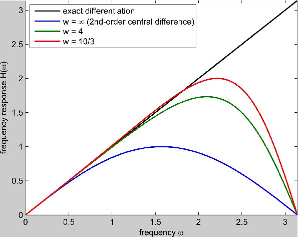
where parameter should be chosen in such a way that (36) delivers a good approximation of , the frequency response for the true derivative. For example, the Taylor series expansion of (36) with respect to at shows that the best approximation of the exact -derivative for is achieved when which corresponds to a Padé approximation. However this choice of parameter is not optimal if we deal with a wider range of frequencies.
Note that (35) is equivalent to an implicit finite difference scheme
| (37) |
Implicit finite differences are widely used for accurate numerical simulations of physical problems involving linear and non-linear wave propagation phenomena, see, for example, [9], [27, Section 5.8]. An implicit finite difference scheme is usually characterized by its frequency-resolving efficiency, the range of frequencies over which a satisfactory approximation of the corresponding differential operator is achieved.
Motivated by [30, 17] where a frequency-based analysis of simple stencils for first-order derivatives was performed, we found out that (36, (37) with deliver a good frequency resolving efficiency for a sufficiently large frequency range, as seen in Figure 7. Of course, the problem of finding an optimal is application-dependent and the optimal value of depends on optimization criteria used and a range of frequencies where the optimization is sought.
The approach via the Minkowski theorem and Veronese map developed in Section 2 is suggestive for an extension of the above results to 3D and to grids in any dimensions. We leave this for future publication.
Acknowledgments. B. K. is grateful to the Ecole Polytechnique in Paris and the Max Planck Institute in Bonn for their hospitality during completion of this paper. He was partially supported by an NSERC research grant. S. T. was partially supported by the Simons Foundation grant No 209361 and by the NSF grant DMS-1105442.
References
- [1] Arnold, V., Khesin, B., 1998. Topological methods in hydrodynamics. Springer.
- [2] Aubert, G., Kornprobst, P., 2006. Mathematical Problems in Image Processing, 2nd Edition. Springer.
- [3] Bannai, E., Bannai, E., 2009. A survey on spherical designs and algebraic combinatorics on spheres. European Journal of Combinatorics 30 (6), 1392–1425.
- [4] Belyaev, A., June 2006. On transfinite barycentric coordinates. In: Proceedings of Fourth Eurographics Symposium on Geometry Processing. Sardinia, Italy, pp. 89–99.
- [5] Bickley, W. G., 1948. Finite difference formulae for the square lattice. Quart. J. Mech. Appl. Math. 1, 35–42.
- [6] Birkhoff, G., Lynch, R. E., 1984. Numerical Solution of Elliptic Problems. SIAM.
- [7] Bradford, J. R., Westhead, D. R., 2005. Improved prediction of protein-protein binding sites using a support vector machines approach. Bioinformatics 21 (8), 1487–1494.
- [8] Childress, S., 1992. Fast dynamo theory. In: Topological aspects of the dynamics of fluids. Kluwer Academic Publishers, Dordrecht, pp. 111–147.
- [9] Colonius, T., Lele, S. K., August 2004. Computational aeroacoustics: progress on nonlinear problems of sound generation. Progress in Aerospace Sciences 40 (6), 345–416.
- [10] Delsarte, P., Goethals, J. M., Seidel, J. J., 1977. Spherical codes and designs. Geometriae Dedicata 6, 363–388.
- [11] Friedman, A., Littman, W., 1962. Functions satisfying the mean value property. Transactions of the American Mathematical Society 102 (1), 167–180.
- [12] Gonzalez, R. C., Woods, R. E., 2008. Digital Image Processing, 3rd Edition. Pearson Prentice Hall.
- [13] Gordon, W., Wixom, J., 1974. Pseudo-harmonic interpolation on convex domains. SIAM J. Numer. Anal. 11 (5), 909–933.
- [14] Hamming, R. W., 1998. Digital Filters, 3rd Edition. Dover.
- [15] Harris, J., 1992. Algebraic Geometry: A First Course. Springer.
- [16] Hong, Y., 1982. On spherical t-designs in . European Journal of Combinatorics 3, 255–258.
- [17] Jähne, B., Scharr, H., Körkel, S., 1999. Principles of filter design. In: Handbook of Computer Vision and Applications, Vol. 2, Signal Processing and Applications. Academic Press, pp. 125–151.
- [18] Kamgar-Parsi, B., Kamgar-Parsi, B., Rosenfeld, A., 1999. Optimally isotropic Laplacian operator. IEEE Transactions on Image Processing 8 (10), 1467–1472.
- [19] Kantorovich, L. V., Krylov, V. I., 1956. Approximate Methods of Higher Analysis. Noordhoff-Interscience.
- [20] Koenderink, J. J., Van Doorn, A. J., 1992. Surface shape and curvature scales. Image and Vision Computing 10, 557–565.
- [21] Langer, T., Belyaev, A., Seidel, H.-P., 2007. Exact and interpolatory quadratures for curvature tensor estimation. Computer Aided Geometric Design 24 (8-9), 443–463.
- [22] Mérigot, Q., Ovsjanikov, M., Guibas, L., 2009. Robust Voronoi-based curvature and feature estimation. In: Proc. of SIAM/ACM Joint Conference on Geometric and Physical Modeling. pp. 1–12.
- [23] Natterer, F., 2001. The Mathematics of Computerized Tomography. SIAM.
- [24] Patra, M., Karttunen, M., 2005. Stencils with isotropic discretisation error for differential operators. Numerical Methods for Partial Differential Equations 22 (4), 936–953.
- [25] Perona, P., Malik, J., 1990. Scale-space and edge detection using anisotropic diffusion. IEEE Transactions on Pattern Analysis and Machine Intelligence 12 (7), 629–639.
- [26] Perona, P., Shiota, T., Malik, J., 1994. Anisotropic Diffusion. Kluwer Academic Press, pp. 73–92.
- [27] Petrila, T., Trif, D., 2005. Basics of Fluid Mechanics and Introduction to Computational Fluid Dynamics. Springer.
- [28] Pottmann, H., Wallner, J., Huang, Q., Yang, Y.-L., 2009. Integral invariants for robust geometry processing. Computer Aided Geometric Design 26, 37–60.
- [29] Pratt, W. K., 2001. Digital Image Processing, 3rd Edition. John Wiley & Sons.
- [30] Scharr, H., Körkel, S., Jähne, B., 1997. Numerische isotropieoptimierung von fir-filtern mittels querglättung. In: Proc. DAGM’97. pp. 367–374.
- [31] Schneider, R., 1993. Convex Bodies: The Brunn-Minkowski Theory. Cambridge University Press.
- [32] Seymour, P. D., Zaslavsky, T., 1984. Averaging sets: A generalization of mean values and spherical designs. Advances in Math. 52, 213224.
- [33] Stroud, A. H., 1971. Approximate Calculation of Multiple Integrals. Prentice-Hall.
- [34] Taubin, G., 1995. Estimating the tensor of curvature of a surface from a polyhedral approximation. In: Proc. ICCV’95. pp. 902–907.
- [35] Valenti, R., Sebe, N., Gevers, T., 2009. Image saliency by isocentric curvedness and color. In: IEEE International Conference on Computer Vision.
- [36] Wardetzky, M., Mathur, S., Kälberer, F., E., G., July 2007. Discrete Laplace operators: No free lunch. In: Proceedings of Fifth Eurographics Symposium on Geometry Processing. Barcelona, Spain, pp. 33–37.
- [37] Weickert, J., 1994. Anisotropic diffusion filters for image processing based quality control. In: Proc. Seventh European Conf. on Mathematics in Industry. Teubner-Verlag, pp. 355–362.
- [38] Weickert, J., 1998. Anisotropic Diffusion in Image Processing. Teubner-Verlag, Stuttgart.
- [39] Weickert, J., Scharr, H., 2002. A scheme for coherence-enhancing diffusion filtering with optimized rotation invariance. Journal of Visual Communication and Image Representation 13, 103–118.
- [40] Zhong, L., Su, Y., Yeo, S.-Y., Tan, R.-S., Ghista, D. N., Kassab, G., 2009. Left ventricular regional wall curvedness and wall stress in patients with ischemic dilated cardiomyopathy. American Journal of Physiology - Heart and Circulatory Physiology 296, H573–H584.