Robust Bayesian reinforcement learning through tight lower bounds

We consider decision making problems where an agent is acting in a (possibly unknown to it) environment. By choosing actions, the agent changes the state of the environment and in addition obtains scalar rewards. The agent acts so as to maximise the expectation of the utility function: $U_{t}\mathrel{\triangleq}\sum_{k=t}^{T}\gamma^{k}r_{k}$, where $\gamma\in[0,1]$ is a discount factor and where the instantaneous rewards $r_{t}\in[0,r_{\textrm{max}}]$ are drawn from a Markov decision process (MDP) $\mu$, defined on a state space ${\mathcal{S}}$ and an action space ${\mathcal{A}}$, both equipped with a suitable metric and $\sigma$-algebra, with a set of transition probability measures $\left\{{\mathcal{T}}_{\mu}^{s,a}\,\middle|\,s\in{\mathcal{S}},a\in{\mathcal{A}}\right\}$ on ${\mathcal{S}}$ , and a set of reward probability measures $\left\{{\mathcal{R}}_{\mu}^{s,a}\,\middle|\,s\in{\mathcal{S}},a\in{\mathcal{A}}\right\}$ on ${\mathbb{R}}$, such that:

where $s_{t}\in{\mathcal{S}}$ and $a_{t}\in{\mathcal{A}}$ are the state of the MDP, and the action taken by the agent at time $t$, respectively. The environment is controlled via a policy $\pi\in\mathcal{P}$. This defines a conditional probability measure on the set of actions, such that $\mathop{\mbox{$\mathbb{P}$}}\nolimits_{\pi}(a_{t}\in A\mid s^{t},a^{t-1})=\pi(A\mid s^{t},a^{t-1})$ is the probability of the action taken at time $t$ being in $A$, where we use $\mathop{\mbox{$\mathbb{P}$}}\nolimits$, with appropriate subscripts, to denote probabilities of events and $s^{t}\mathrel{\triangleq}s_{1},\ldots,s_{t}$ and $a^{t-1}\mathrel{\triangleq}a_{1},\ldots,a_{t-1}$ denotes sequences of states and actions respectively. We use $\mathcal{P}_{k}$ to denote the set of $k$-order Markov policies. Important special cases are the set of blind policies $\mathcal{P}_{0}$ and the set of memoryless policies $\mathcal{P}_{1}$. A policy in $\pi\in\bar{\mathcal{P}}_{k}\subset\mathcal{P}_{k}$ is stationary, when $\pi(A\mid s_{t-k+1}^{t},a_{t-k+1}^{t-1})=\pi(A\mid s^{k},a^{k-1})$ for all $t$.

The expected utility, conditioned on the policy, states and actions is used to define a value function for the MDP $\mu$ and a stationary policy $\pi$, at stage $t$:

where the expectation is taken with respect to the process defined jointly by $\mu,\pi$ on the set of all state-action-reward sequences $({\mathcal{S}},{\mathcal{A}},{\mathbb{R}})^{*}$. The optimal value function is denoted by $Q^{*}_{\mu,t}\mathrel{\triangleq}\sup_{\pi}Q^{\pi}_{\mu,t}$ and $V^{*}_{\mu,t}\mathrel{\triangleq}\sup_{\pi}V^{\pi}_{\mu,t}$. We denote the optimal policy¹¹ 1 We assume that there exists at least one optimal policy. If there are multiple optimal policies, we choose arbitrarily among them. for $\mu$ by $\pi_{\mu}^{*}$. Then $Q^{*}_{\mu,t}=Q^{\pi_{\mu}^{*}}_{\mu,t}$ and $V^{*}_{\mu,t}=V^{\pi_{\mu}^{*}}_{\mu,t}$.

There are two ways to handle the case when the true MDP is unknown. The first is to consider a set of MDPs such that the probability of the true MDP lying outside this set is bounded from above [20, 21, 4, 19, 28, 27, e.g.]. The second is to use a Bayesian framework, whereby a full distribution over possible MDPs is maintained, representing our subjective belief, such that MDPs which we consider more likely have higher probability [14, 10, 31, 2, 12, e.g.]. Hybrid approaches are relatively rare [16]. In this paper, we derive a method for efficiently calculating near-optimal, robust, policies in a Bayesian setting.

Even when our belief $\xi$ is a probability measure over a finite set of MDPs $\mathcal{M}$, the finding an optimal policy is intractable. For that reason, we restrict ourselves to memoryless policues $\pi\in\mathcal{P}_{1}$. We can approximate the optimal memoryless policy with respect to $\xi$, by setting the posterior measure given knowledge of the policy so far and the current state, to equal the initial belief, i.e. $\xi(\mu\mid s_{t}=s,\pi)=\xi(\mu)$ (we do not condition on the complete history, since the policies are memoryless). The approximation is in practice quite good, since the difference between the two measures tends to be small. The policy $\pi_{\textsc{MMBI}}$ can then be obtained via the following backwards induction. By definition:

where the expected reward term can be written as

The next-step utility can be written as:

Putting those steps together, we obtain Algorithm 1, which greedily calculates a memoryless policy for a $T$-stage problem and returns its expected utility.

The calculation is greedy, since optimising over $\pi$ implies that at any step $t+k$, we must condition the belief on past policy steps $\xi(\mu\mid s_{t+k}=s,\pi_{t},\ldots,\pi_{t+k-1})$ to calculate the expected utility correctly. Thus, the optimal $\pi_{t+k}$ depends on both future and past selections. Nevertheless, it is easy to see that Alg. 1 returns the correct expected utility for time step $t$. Theorem 2.1 bounds the gap between this and the Bayes-optimal value function when the difference between the current and future beliefs is small.

We can similarly bound the gap between the MMBI policy and the $\xi$-optimal memoryless policy, by bounding $\sup_{k,s,\pi}\|\xi_{t}(\cdot)-\xi_{t}(\cdot\mid s_{k}=s,\pi)\|_{\lambda,1}$.

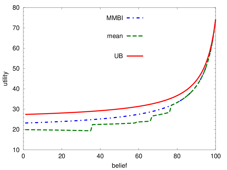
The $\xi$-optimal memoryless policy is generally different from the policy which is optimal with respect to the expected MDP $\hat{\mu}_{\xi}\mathrel{\triangleq}\mathop{\mbox{$\mathbb{E}$}}\nolimits_{\xi}\mu$, as can be seen via counterexample where $\mathop{\mbox{$\mathbb{E}$}}\nolimits_{\xi}V^{\pi}_{\mu}\neq V^{\pi}_{\hat{\mu}_{\xi}}$, or even where $\mathop{\mbox{$\mathbb{E}$}}\nolimits_{\xi}\mu\notin\mathcal{M}$. MMBI can be used to obtain a much tighter value function bound than the $\hat{\mu}_{\xi}$-optimal policy, as shown in Fig. 1, where the MMBI bound is compared to the $\hat{\mu}_{\xi}$-optimal policy bound and the simple upper bound: $V^{*}_{\xi}(s)\leq\mathop{\mbox{$\mathbb{E}$}}\nolimits_{\xi}\max_{\pi}V^{\pi}_{\mu}(s)$. The figure shows how the bounds change as our belief over 8 MDPs changes. When we are more uncertain, MMBI is much tighter than $\hat{\mu}_{\xi}$-optimal. However, when most of the probability mass is around a single MDP, both lower bounds coincide. In further experiments on online reinforcement learning, described in Sec. 3, near-optimal memoryless policies are compared against the $\hat{\mu}_{\xi}$-optimal policy.

Selecting the number of samples $n$ according to $\epsilon$ for MCBRL is computationally prohibitive. In practice, instead of setting $n$ via $\epsilon$, we simply consider increasing values of $n$. For a single sample ($n=1$), MCBRL is equivalent to the sampling method in [29], which at every new stage, samples a single MDP from the current posterior and then uses the policy that is optimal for the sampled MDP. In addition, for this particular experiment, rather than using the memoryless policy found, we apply the stationary policy derived by using the first step of the memoryless policy. This incurs a small additional loss.

We also compared MCBRL against the common heuristic of acting according to the policy that is optimal with respect to the expected MDP $\hat{\mu}_{\xi}\mathrel{\triangleq}\mathop{\mbox{$\mathbb{E}$}}\nolimits_{\xi}\mu$. The algorithm, referred to as the Exploit heuristic in [23], is shown in detail in Alg. 4. At every step, this calculates the expected MDP by obtaining the expected transition kernel and reward function under the current belief. It then acts according to the optimal policy with respect to $\hat{\mu}_{\xi}$. This policy may be much worse than the optimal policy, even within the class of stationary policies $\bar{\mathcal{P}}_{1}$.

We compared the algorithms on the Chain task [9], commonly used to evaluate exploration in reinforcement learning problems. Traditionally, the task has a horizon of $10^{3}$ steps, a discount factor $\gamma=0.95$, and the expected total reward $\mathop{\mbox{$\mathbb{E}$}}\nolimits_{\mu,\pi}\sum_{t=1}^{T}r_{t}$ is compared. We also report the expected utility $\mathop{\mbox{$\mathbb{E}$}}\nolimits_{\mu,\pi}U_{t}$, which depends on the discount factor. All quantities are estimated over $10^{4}$ runs with appropriately seeded random number generators to reduce variance.²² 2 In both cases this expectation is with respect to the distribution induced by the actual MDP $\mu$ and policy $\pi$ followed, rather than with respect to the belief $\xi$. The initial belief about the state transition distribution was set to be a product-Dirichlet prior [11, see] with all parameters equal to $|{\mathcal{S}}|^{-1}$, while a product-Beta prior with parameters $(1,1)$ was used for the rewards.

Figure 2 summarises the results in terms of total reward. The left hand side (2(a)) shows the expected difference in total reward between the optimal policy $\pi^{*}$ and the used policy $\pi$, over $T$ steps, i.e. the regret: ${\mathcal{L}}=\mathop{\mbox{$\mathbb{E}$}}\nolimits_{\mu,\pi}\sum_{t=1}^{T}r_{t}-\mathop{\mbox{$\mathbb{E}$}}\nolimits_{\mu,\pi}\sum_{t=1}^{T}r_{t}$. The error bars denote $95\%$ confidence intervals obtained via a $10^{4}$-bootstrap [15]. For $n=1$, MCBRL performs worse than the expected MDP approach, in terms of total reward. On the other hand, as the number of samples increase, its performance monotonically improves.

Some more detail on the behaviour of the algorithms is given in Figure 2(b), which shows the empirical performance distribution in terms of total reward. The expected MDP approach has a high probability of getting stuck in a sub-optimal regime. On the contrary, MCBRL, for $n=1$, results in significant over-exploration of the environment. However, as $n$ increases, MCBRL explores significantly less, while the number of runs where we are stuck in the sub-optimal regime remains small ($<1\%$ of the runs).

Table 1 presents comparative results on the chain task for Alg. 4 and for MCBRL for $n\in\{1,8,16\}$ in terms of the total reward received in $10^{3}$ steps. This enables us to compare against the results reported in [23, 17]. While the performance of Alg. 4 may seem surprisingly good, it is actually in line with the results reported in [23]. Therein, Beetle only outperformed Alg. 4 in the Chain task when stronger priors were used. In addition, we would like to note that while the case $n=1$ is worse than Alg. 4 for the total reward metric, this no longer holds when we examine the expected utility, where an improvement can already be seen for $n=1$.

We introduced MMBI, a simple backwards induction procedure, to obtain a near-optimal memoryless policy with respect to a belief over a finite number of MDPs. This was generalised to MSBI, a stochastic procedure, whose loss is close in expectation to MMBI, with a gap that depends polynomially on the number of samples, for a belief on arbitrary set of MDPs. It is shown that MMBI results in a much tighter lower bound on the value function that the value of the $\hat{\mu}_{\xi}$-optimal policy. In addition, we prove a bound on the gap between the value of the MMBI policy and the Bayes-optimal policy. Our results are then applied to reinforcement learning problems, by using the MCBRL algorithm to sample a number of MDPs at regular intervals. This can be seen as a principled generalisation of [29], which only draws one sample at each such interval. Then MSBI is used to calculate a near-optimal memoryless policy within each interval. We show experimentally that this performs significantly better than following the $\hat{\mu}_{\xi}$-optimal policy. It is also shown that the performance increases as we make the bound tighter by increasing the number of samples taken.

Compared to results reported for other Bayesian reinforcement learning approaches on the Chain task, this rather simple method performs surprisingly well. This can be attributed to the fact that at each stage, the algorithm selects actions according to a nearly-optimal stationary policy.

In addition, MSBI itself could be particularly useful for inverse reinforcement learning problems (see for example [1, 22]) where the underlying dynamics are unknown, or to multi-task problems[26]. Then it would be possible to obtain good stationary policies that take into account the uncertainty over the dynamics, which should be better than using the expected MDP heuristic. More specifically, in future work, MMBI will be used to generalise the Bayesian methods developed in [13, 25] for the case of unknown dynamics.

In terms of direct application to reinforcement learning, MSBI could be used in the inner loop of some more sophisticated method than MCBRL. For example, it could be employed to obtain tight lower bounds for the leaf nodes of a planning tree such as[12]. By tight integration with such methods, we hope to obtain improved performance, since we would be considering wider policy classes. In a related direction, it would be interesting to see examine better upper bounds [8, 7, 24] and in particular whether the information relaxations discussed by Brown et al. [5] could be extended to the Bayes-optimal case.

Many thanks to Matthijs Snel and Shimon Whiteson for extensive discussions on the optimality of the MMBI algorithm, and for helping to discover an error. In addition, I would like to thank Nikos Vlassis and the anonymous reviewers for helpful comments. This work was partially supported by the EU-Project IM-CLeVeR, FP7-ICT-IP-231722, and the Marie Curie Project ESDEMUU, Grant Number 237816.

References

- [1] P. Abbeel and A.Y. Ng. Apprenticeship learning via inverse reinforcement learning. In Proceedings of the 21st international conference on Machine learning (ICML 2004), 2004.
- [2] J. Asmuth, L. Li, M. L. Littman, A. Nouri, and D. Wingate. A Bayesian sampling approach to exploration in reinforcement learning. In UAI 2009, 2009.
- [3] Peter Auer, Thomas Jaksch, and Ronald Ortner. Near-optimal regret bounds for reinforcement learning. In Proceedings of NIPS 2008, 2008.
- [4] R.I. Brafman and M. Tennenholtz. R-max-a general polynomial time algorithm for near-optimal reinforcement learning. The Journal of Machine Learning Research, 3:213–231, 2003.
- [5] D. B. Brown, J. E. Smith, and P. Sun. Information relaxations and duality in stochastic dynamic programs. Operations Research, 58(4):785–801, 2010.
- [6] P. Castro and D. Precup. Smarter sampling in model-based bayesian reinforcement learning. Machine Learning and Knowledge Discovery in Databases, pages 200–214, 2010.
- [7] D. P. de Farias and B. Van Roy. The linear programming approach to approximate dynamic programming. Operations Research, 51(6):850–865, 2003.
- [8] D. P. de Farias and B. Van Roy. On constraint sampling in the linear programming approach to approximate dynamic programming. Mathematics of Operations Research, 293(3):462–478, 2004.
- [9] Richard Dearden, Nir Friedman, and Stuart J. Russell. Bayesian Q-learning. In AAAI/IAAI, pages 761–768, 1998.
- [10] Richard Dearden, Nir Friedman, and David Andre. Model based Bayesian exploration. In Kathryn B. Laskey and Henri Prade, editors, Proceedings of the 15th Conference on Uncertainty in Artificial Intelligence (UAI-99), pages 150–159, San Francisco, CA, July 30–August 1 1999. Morgan Kaufmann, San Francisco, CA.
- [11] Morris H. DeGroot. Optimal Statistical Decisions. John Wiley & Sons, 1970.
- [12] Christos Dimitrakakis. Complexity of stochastic branch and bound methods for belief tree search in Bayesian reinforcement learning. In 2nd international conference on agents and artificial intelligence (ICAART 2010), pages 259–264, Valencia, Spain, 2009. ISNTICC, Springer.
- [13] Christos Dimitrakakis and Constantin A. Rothkopf. Bayesian multitask inverse reinforcement learning. In European Workshop on Reinforcement Learning (EWRL 2011), 2011.
- [14] Michael O’Gordon Duff. Optimal Learning Computational Procedures for Bayes-adaptive Markov Decision Processes. PhD thesis, University of Massachusetts at Amherst, 2002.
- [15] Bradley Efron and Robert J. Tibshirani. An Introduction to the Bootstrap, volume 57 of Monographs on Statistics & Applied Probability. Chapmann & Hall, November 1993. ISBN 0412042312.
- [16] Mahdi Milain Fard and Joelle Pineau. PAC-Bayesian model selection for reinforcement learning. In NIPS 2010, 2010.
- [17] Thomas Furmston and David Barber. Variational methods for reinforcement learning. In Yee Whye Teh and Mike Titterington, editors, Proceedings of the 13th International Conference on Artificial Intelligence and Statistics (AISTATS), volume 9 of JMLR : W&CP, pages 241–248.
- [18] C. J. Gittins. Multi-armed Bandit Allocation Indices. John Wiley & Sons, New Jersey, US, 1989.
- [19] Thomas Jacksh, Ronald Ortner, and Peter Auer. Near-optimal regret bounds for reinforcement learning. Journal of Machine Learning Research, 11:1563–1600, 2010.
- [20] Leslie Pack Kaelbling. Learning in Embedded Systems. PhD thesis, ept of Computer Science, Stanford, 1990.
- [21] Michael Kearns and Satinder Singh. Near-optimal reinforcement learning in polynomial time. In Proc. 15th International Conf. on Machine Learning, pages 260–268. Morgan Kaufmann, San Francisco, CA, 1998.
- [22] Andrew Y. Ng and Stuart Russell. Algorithms for inverse reinforcement learning. In in Proc. 17th International Conf. on Machine Learning, pages 663–670. Morgan Kaufmann, 2000.
- [23] P. Poupart, N. Vlassis, J. Hoey, and K. Regan. An analytic solution to discrete Bayesian reinforcement learning. In ICML 2006, pages 697–704. ACM Press New York, NY, USA, 2006.
- [24] L. C. G. Rogers. Pathwise stochastic optimal control. SIAM Journal on Control and Optimization, 46(3):1116–1132, 2008.
- [25] Constantin A. Rothkopf and Christos Dimitrakakis. Preference elicitation and inverse reinforcement learning. In European Conference on Machine Learning (ECML 2011), 2011.
- [26] M. Snel and S. Whiteson. Multi-Task Reinforcement Learning: Shaping and Feature Selection, EWRL 2011, 2011.
- [27] A.L. Strehl and M.L. Littman. An analysis of model-based interval estimation for Markov decision processes. Journal of Computer and System Sciences, 74(8):1309–1331, 2008.
- [28] A.L. Strehl, L. Li, and M.L. Littman. Reinforcement learning in finite MDPs: PAC analysis. The Journal of Machine Learning Research, 10:2413–2444, 2009.
- [29] Malcolm Strens. A bayesian framework for reinforcement learning. In ICML 2000, pages 943–950. Citeseer, 2000.
- [30] Tao Wang, Daniel Lizotte, Michael Bowling, and Dale Schuurmans. Bayesian sparse sampling for on-line reward optimization. In ICML ’05, pages 956–963, New York, NY, USA, 2005. ACM.
- [31] J. Wyatt. Exploration control in reinforcement learning using optimistic model selection. In A. Danyluk and C. Brodley, editors, Proceedings of the Eighteenth International Conference on Machine Learning, 2001.