On the importance of the 1-loop finite
corrections to seesaw neutrino masses

Neutrino oscillation experiments have firmly established that neutrino have tiny but non-zero masses and that the mixing in the leptonic sector is in sharp contrast with the small mixing that characterizes the quark sector [1, 2]. From a theoretical perspective the smallness of neutrino masses can be well understood within the seesaw model [3, 4, 5, 6, 7], in which the fermion sector of the Standard Model is extended by adding new electroweak fermionic singlets (standard seesaw model). In this framework, light neutrino masses are generated via mixing with the singlet states and their smallness can naturally be explained if the singlets masses are very large.

The determination of the regions of parameter space consistent with low energy neutrino observables in the seesaw model typically relies on parametrizations of the neutrino Yukawa couplings [8, 9]. Once the Yukawas are properly parametrized, such regions are found by doing numerical scans in which the neutrino experimental data is used as an input. This procedure is always based on the tree-level light neutrino mass matrix and fails if in some regions of the parameter space the one-loop corrections to the tree-level mass matrix turn out to have sizable values.

The one-loop corrections to the seesaw light neutrino mass matrix were first discussed in [10] in a general setup with an arbitrary number of singlets, lepton doublets and Higgs doublets. They were later analyzed in ref. [11] in a particular realization in which, due to a particular Yukawa mass matrix, light neutrino masses vanish at tree-level and are entirely generated by the one-loop corrections. Subsequently, the renormalization of general theories with Dirac and/or Majorana neutrinos was carried out in [12] and additional studies were done in references [13, 14, 15, 16, 17].

Loop corrections are of two types: renormalizable and intrinsically finite. The renormalizable pieces consist of corrections to the tree level parameters already present in the seesaw Lagrangian, and are suppressed with respect to the tree level piece by extra Yukawa couplings and by the loop factor 1/16$\pi^{2}$. The finite parts instead are corrections to the vanishing elements of the tree-level mass matrix for the neutral fermions, and are only suppressed by the loop factor. Thus, they are potentially large.

The aim of this paper is to quantify the impact that the finite one-loop corrections might have on the effective light neutrino mass matrix. We consider the most general standard seesaw model and numerically analyze the importance of these corrections for the different mass matrix elements as well as for the neutrino mass eigenvalues and mixing angles, differentiating in our discussion between the normal and the inverted light neutrino mass spectrum. We will show that the corrections can range over several orders of magnitude, depending on whether one relies or not on models where consistency with the measured neutrino masses and mixing angles requires strong cancellations in the tree-level neutrino mass matrix. Indeed, as we will discuss, once one-loop corrections are taken into account these models are barely reconcilable with data. Barring these cases, we will prove that the finite corrections are usually of order $~20-40\%$ but they may exceed the tree-level value for certain entries that can be strongly suppressed. In order to make reliable predictions in the seesaw, therefore, the finite one-loop corrections should be included.

The rest of the paper is organized as follows: in section 2 we define our notation and briefly describe the seesaw model at tree-level, including its standard parametrization. We discuss the finite 1-loop corrections in section 3. In sections 4 and 5 our main results are presented –the calculation of the finite corrections for the normal and inverted light neutrino mass spectrum. Then, we consider the particular case of tribimaximal mixing in section 6 and we determined how such mixing pattern is modified by the 1-loop finite corrections. A brief discussion of our results and some comments on their possible phenomenological implications is given in section 7. In section 8 we draw our conclusions and summarize our findings. For completeness, in the appendix we present the details of the calculation of the finite one-loop corrections.

In the standard seesaw model, three fermionic electroweak singlets $N_{R_{i}}$ are added to the Standard Model. In the basis in which the matrix of charged lepton Yukawa couplings and the singlet mass matrix are diagonal the Lagrangian accounting for the new interactions can be written as

$$-{\cal L}=-i\bar{N}_{R_{i}}\,{\partial\!\!\!\!\diagup}N_{R_{i}}+\tilde{\phi}^{\dagger}\bar{N}_{R_{i}}\lambda_{ij}\ell_{Lj}+\frac{1}{2}\bar{N}_{R_{i}}CM_{R_{i}}\bar{N}_{R}^{T}+\mbox{h.c.}$$

(1)

where $\phi^{T}=(\phi^{+}\phi^{0})$ is the Higgs electroweak doublet, $\ell_{L}$ are the leptonic $SU(2)$ doublets, $C$ is the charge conjugation operator and $\mathbf{\lambda}$ is a Yukawa matrix in flavor space. In the left-handed chiral basis $\mathbf{n_{L}}^{T}=(\mathbf{\nu_{L}},(\mathbf{N_{R}})^{C})^{T}$, and once electroweak symmetry breaking is taken into account, the neutral fermion mass terms can be written as

$$-{\cal L}_{F^{0}}=\frac{1}{2}\mathbf{n}_{\mathbf{L}}^{T}C\mathbf{\cal M}\,\mathbf{n_{L}}+\mbox{h.c.}$$

(2)

where $\mathbf{\cal M}$, the $6\times 6$ neutral fermion mass matrix, is given by

$$\mathbf{\cal M}=\begin{pmatrix}[cc]\mathbf{0~}&\mathbf{M}_{\mathbf{D}}^{T}\\ \mathbf{M_{D}}&\mathbf{\hat{M}_{R}}\end{pmatrix}\,,$$

(3)

with $\mathbf{M_{D}}=v\mathbf{\lambda}$ ($v=\sqrt{2}M_{W}/g\simeq 174$ GeV). The mass spectrum is obtained by rotating the fields to the mass eigenstate basis, denoted by $\chi_{i}$, via the unitary matrix $\mathbf{U}$:

$$\mathbf{\chi_{L}}=\mathbf{U}^{\dagger}\mathbf{n_{L}}\,.$$

(4)

In this basis, the Lagrangian mass terms, equation (2), become

$$-{\cal L}_{F^{0}}=\frac{1}{2}\overline{\mathbf{\chi}}\,\mathbf{\hat{\cal M}}P_{L}\,\mathbf{\chi}+\text{h.c.}$$

(5)

where

$$\mathbf{U}^{T}\,\mathbf{\cal M}\,\mathbf{U}=\mathbf{\hat{\cal M}}=\mbox{diag}(m_{\chi_{1}},\dots m_{\chi_{6}})$$

(6)

and $\chi_{i}$ are the physical Majorana neutrino fields. Note that by decomposing the matrix $\mathbf{U}$ as [10, 17, 16]

$$\mathbf{U}=\begin{pmatrix}[l]\mathbf{U_{L}}\\ \mathbf{U}_{\mathbf{R}}^{*}\end{pmatrix}$$

(7)

the $\nu_{L_{i}}$ and $N_{R_{i}}$ states can be expressed as

$$\nu_{L_{i}}=U_{L_{i}j}P_{L}\chi_{j}\,,\quad N_{R_{i}}=U_{R_{ij}}P_{R}\chi_{j}\,.$$

(8)

In the seesaw limit ($\mathbf{M_{D}}\ll\mathbf{M_{R}}$), the diagonalization of the mass matrix (3) gives rise to a split spectrum consisting of three heavy states with masses $M_{R_{i}}$ and three light states with an effective mass matrix, $\mathbf{m}_{\boldsymbol{\nu}}^{\mbox{\tiny(tree)}}$, given by

$$\mathbf{m}_{\boldsymbol{\nu}}^{\mbox{\tiny(tree)}}=-\mathbf{M}_{\mathbf{D}}^{T}\,\mathbf{\hat{M}_{R}}^{-1}\,\mathbf{M_{D}}\,.$$

(9)

The light neutrino mass spectrum, mixing angles and CP violating phases –the so-called low-energy observables– are obtained from this matrix after diagonalization:

$$\mathbf{U}_{\ell}^{T}\mathbf{m}_{\boldsymbol{\nu}}^{\mbox{\tiny(tree)}}\mathbf{U}_{\ell}=\mathbf{\hat{m}_{\nu}}\,,$$

(10)

where $\mathbf{U_{\ell}}$ is the leptonic mixing matrix parametrized according to

$$\mathbf{U_{\ell}}=\mathbf{U_{\ell}}(\theta_{23})\mathbf{U_{\ell}}(\theta_{13},\delta)\mathbf{U_{\ell}}(\theta_{12})\times\mbox{diag}(e^{-i\varphi_{1}},e^{-i\varphi_{2}},1)$$

(11)

with $\delta,\varphi_{1,2}$ being respectively the Dirac and Majorana CP violating phases and $U_{\ell}(\theta)$ rotation matrices.

The determination of the seesaw parameters compatible with neutrino experimental data relies on parametrizations of the Yukawa couplings or, equivalently, of the Dirac neutrino mass matrix, $\mathbf{M_{D}}=v\,\mathbf{\lambda}$. In the numerical analysis of the finite one-loop corrections, we have used the most common parametrization of the seesaw, the Casas-Ibarra parametrization [8]. In this parametrization, the most general $\mathbf{M_{D}}$ compatible with eq. (9) is given by

$$\mathbf{M_{D}}=i\,\mathbf{\hat{M}_{R}}^{1/2}\,\mathbf{R}\,\mathbf{\hat{m}_{\nu}}^{1/2}\,\mathbf{U_{\ell}}^{\dagger}\;,$$

(12)

where $\mathbf{R}$ is any orthogonal matrix. This matrix can be written as a rotation matrix determined by three complex angles.

The neutrino mass eigenvalues and the mixing matrix entering into this equation are strongly constrained by experimental data whereas the masses of the singlet neutrinos and the matrix $\mathbf{R}$ are entirely free parameters of the seesaw model. In the numerical treatment of our results (sections 4 and 5) we also impose the perturbativity condition suggested recently in [18]:

$$\mathrm{Tr}\left[\mathbf{\lambda}^{\dagger}\mathbf{\lambda}\right]\leq 3.$$

(13)

Now that we have reviewed the seesaw mechanism at tree level, let us take a look at the 1-loop corrections to neutrino masses.

In the standard seesaw, the one-loop corrections to the $\nu-N$ mass matrix are determined by the neutrino interactions with the $Z$ boson, the neutral Goldstone bosons ($G^{0}$), and the Higgs boson ($h^{0}$) –see appendix A. All together, in addition to the correction involving the standard model leptonic charged current, they define the one-loop two point function $-i\mathbf{\Sigma}(p)$ [17].

Once the one-loop corrections are taken into account the neutral fermion mass matrix is given by

$$\mathbf{\cal M}=\mathbf{\cal M}^{{\mbox{\tiny(tree)}}}+\mathbf{\cal M}^{{\mbox{\tiny(1-loop)}}}\,,$$

(14)

where the 1-loop contribution can be decomposed as

$$\mathbf{{\cal M}}^{{\mbox{\tiny(1-loop)}}}=\begin{pmatrix}\mathbf{\delta M_{L}}&\mathbf{\delta M}_{\mathbf{D}}^{T}\\ \mathbf{\delta M_{D}}&\mathbf{\delta M_{R}}\end{pmatrix}\,.$$

(15)

Notice that the $\mathbf{0}_{3\times 3}$ matrix appearing at tree-level is replaced by the contribution $\mathbf{\delta M_{L}}$, which among all the sub-matrices in $\mathbf{{\cal M}}^{\mbox{\tiny(1-loop)}}$ is the dominant one [17].

Neglecting the subdominant pieces in $\mathbf{{\cal M}}^{\mbox{\tiny(1-loop)}}$ and after block diagonalization of the neutral fermion mass matrix, the effective light neutrino mass matrix, up to one-loop order, can be written as

$$\mathbf{m_{\nu}}=\mathbf{m}_{\nu}^{\mbox{\tiny(tree)}}+\mathbf{m}_{\boldsymbol{\nu}}^{\mbox{\tiny(1-loop)}}=-\mathbf{M}_{\mathbf{D}}^{T}\,\mathbf{\hat{M}_{R}}^{-1}\,\mathbf{M_{D}}+\mathbf{\delta M_{L}}\,.$$

(16)

The sub-matrix $\mathbf{\delta M_{L}}$ and all the other sub-matrices entering in $\mathbf{\cal M}^{{\mbox{\tiny(1-loop)}}}$ are entirely determined by the self-energy functions $\mathbf{\Sigma_{L}^{S}}(p^{2})$ (see appendix A) via the diagonalization relation (6):

$$\mathbf{\cal M}^{{\mbox{\tiny(1-loop)}}}=\mathbf{U}^{*}\mathbf{\Sigma_{L}^{S}}(p^{2})\mathbf{U}^{\dagger}\,.$$

(17)

Accordingly, the finite contribution is given by

$$\mathbf{\delta M_{L}}=\mathbf{U_{L}}^{*}\mathbf{\Sigma^{S}_{L}}(p^{2})\mathbf{U_{L}}^{\dagger}=\mathbf{U_{L}}^{*}\mathbf{\Sigma^{S}_{L}}(0)\mathbf{U_{L}}^{\dagger}\,,$$

(18)

where we have used the fact that $\mathbf{\Sigma^{S}_{L}}$ can be evaluated at zero external momentum [17]. The self-energy functions $\mathbf{\Sigma^{S}_{L}}(0)$ are determined by three Feynman self-energy diagrams involving the $Z$, the neutral Goldstone boson $G^{0}$ and the Higgs boson $h^{0}$. Each diagram contains a divergent piece but when summing up the three contributions the result turns out to be finite, as it has to be since there are no counterterms that would allow to absorb a possible divergence (see appendix A for more details). The final expression for the finite one-loop correction is given by[17]

$$\mathbf{\delta M_{L}}=\mathbf{M}_{\mathbf{D}}^{T}\mathbf{\hat{M}_{R}}^{-1}\left\{\frac{g^{2}}{64\pi^{2}M_{W}^{2}}\left[m_{h}^{2}\ln\left(\frac{\mathbf{\hat{M}_{R}}^{2}}{m^{2}_{h}}\right)+3M_{Z}^{2}\ln\left(\frac{\mathbf{\hat{M}_{R}}^{2}}{M^{2}_{Z}}\right)\right]\right\}\mathbf{M_{D}}\,.$$

(19)

Notice that this correction is not suppressed, with respect to tree-level result, by additional factors of $M_{D}/M_{R}$. Thus, it is expected to be smaller than the tree-level mass term solely by a factor of order $(16\pi^{2})^{-1}\ln(M_{R}/M_{Z})$.

In spite of the similar structure of the 1-loop correction and the tree-level result, they are not proportional to each other unless the heavy neutrinos are degenerate –$\mathbf{M_{R}}\propto\mathbf{I}$. Hence, one could in principle have that $\mathbf{m}_{\nu}^{\mbox{\tiny(tree)}}=0$ and that neutrino masses arise entirely from 1-loop effects, as proposed in [11]. Such models, however, are rather contrived and will not be discussed in the following. We are interested, instead, in the generic modifications to the neutrino mass matrix induced by the 1-loop corrections.

To evaluate these corrections, we first find sets of $\mathbf{M_{D}}$ and $\mathbf{\hat{M}_{R}}$ compatible with the experimental data at tree-level –using equation(12)– and then use them to evaluate $\mathbf{\delta M_{L}}$^aa a Alternatively, one could choose the seesaw parameters so that at 1-loop they are compatible with the experimental data. Both procedures give rise to the same effects.. Specifically, we generate the diagonal matrix of light neutrino masses (according to the desired spectra: normal or inverted) and the mixing matrix $\mathbf{U}_{\ell}$ such that they are compatible with neutrino data. For simplicity, the phases in $\mathbf{U_{\ell}}$ were assumed to vanish. Then, we randomly generate the three masses of the heavy states (in the range $1$ TeV to $10^{12}$ GeV) and the elements of the orthogonal matrix $\mathbf{R}$. From equation (12), we can then obtain $\mathbf{M_{D}}$, which together with the generated $\mathbf{M_{R}}$ allows us to evaluate $\mathbf{\delta M_{L}}$^bb b In our analysis we fix $m_{h^{0}}=150$ GeV.. The size of the corrections is then determined by the ratio between the contributions up to 1-loop order and the tree-level result for the different elements of the neutrino mass matrix, $(\mathbf{m}_{\nu}^{\mbox{\tiny(tree)}}+\mathbf{m}_{\nu}^{\mbox{\tiny(1-loop)}})/\mathbf{m}_{\nu}^{\mbox{\tiny(tree)}}$.

In the next two sections our main results are presented: we compute the corrections to the neutrino mass matrix in the seesaw model for the two different kinds of light neutrino spectra, with normal and inverted hierarchy.

If the spectrum of light neutrinos has a normal hierarchy ($m_{\nu_{3}}=\sqrt{\Delta m_{atm}^{2}}$, $m_{\nu_{2}}=\sqrt{\Delta m_{sol}^{2}}$, $m_{\nu_{1}}\ll m_{\nu_{2}},m_{\nu_{3}}$), the elements of the neutrino mass matrix take values within the following ranges:

$$\mathbf{m}_{\nu}^{\mbox{\tiny{exp}}}=\left(\begin{array}[]{rrr}(2.5,5.5)\times 10^{-12}&(2.3,9.8)\times 10^{-12}&(-3.3,4.9)\times 10^{-12}\\ -&(2.0,3.4)\times 10^{-11}&(1.9,2.3)\times 10^{-11}\\ -&-&(2.1,3.4)\times 10^{-11}\end{array}\right)\,\mbox{GeV}$$

(20)

as the oscillation parameters vary within their $2$-$\sigma$ experimentally allowed intervals [2, 1]. Since the matrix is symmetric, we only show the six independent matrix elements. Notice, in particular, that the element ($1,3$) is the only one that can vanish in this case. It can be easily checked that this can happen if $\theta_{13}$ is between $4^{\circ}$ and $6^{\circ}$. All other elements vary within a relatively small range –not so small for (1,2)– between $10^{-11}$ and $10^{-12}$ GeV. Since the corrections to the neutrino mass matrix are not proportional to the matrix element itself, the correction to the element ($1,3$) could easily exceed its tree-level value.

With the aim of facilitating the study of these corrections and the understanding of their origin, we will divide our analysis in two parts depending on what is assumed for the orthogonal matrix $\mathbf{R}$. First it is taken to be real and then the most general case is considered, a complex matrix. The number of free parameters will therefore increase as we move from the first case to the second.

If the spectrum of light neutrinos has an inverted hierarchy (IH), $m_{\nu_{2}}=\sqrt{\left|\Delta m_{atm}^{2}\right|}$, $m_{\nu_{1}}=\sqrt{\left|\Delta m_{atm}^{2}\right|-\Delta m_{sol}^{2}}$, $m_{\nu_{3}}\ll m_{\nu_{2}},m_{\nu_{1}}$, the elements of the neutrino mass matrix take values within the following ranges:

$$\mathbf{m_{\nu}}^{\mbox{\tiny{exp}}}=\left(\begin{array}[]{rrr}(4.5,5.1)\times 10^{-11}&(-8.5,1.7)\times 10^{-12}&(-8.5,1.3)\times 10^{-12}\\ -&(1.7,3.3)\times 10^{-11}&(-2.5,-2.0)\times 10^{-11}\\ -&-&(1.8,3.4)\times 10^{-11}\par\end{array}\right)\,\mbox{GeV}$$

(21)

as the oscillation parameters vary within their $2$-$\sigma$ experimentally allowed intervals [2, 1]. Notice that in this case the elements ($1,2$) and ($1,3$) are both allowed to vanish, an event that can happen if $\theta_{13}$ is smaller than about $2^{\circ}$. We expect, therefore, large fractional corrections to the entries ($1,2$) and ($1,3$) of the neutrino mass matrix independently of $\mathbf{R}$. As before, we will divide the analysis of the 1-loop corrections into two parts: $\mathbf{R}$ real and $\mathbf{R}$ complex.

We would like now to apply the ideas discussed in the previous sections to a particular and well-motivated scenario: seesaw models with tribimaximal mixing (see e.g. [19]). In scenarios with tribimaximal mixing, the neutrino mixing matrix is given at tree level by

$$U_{\ell}=\left(\begin{array}[]{ccc}\sqrt{2/3}&1/\sqrt{3}&0\\ -1/\sqrt{6}&1/\sqrt{3}&-1/\sqrt{2}\\ -1/\sqrt{6}&1/\sqrt{3}&1/\sqrt{2}\end{array}\right)\,.$$

(22)

As a result, the mixing angles take the values $\theta_{12}=35.3^{\circ}$, $\theta_{23}=45^{\circ}$, $\theta_{13}=0$ at tree level. One may therefore wonder how they would change once the finite one-loop corrections to the seesaw neutrino mass matrix that we have studied are taken into account^dd d Additional corrections from other sources may also be important but are not considered here.. For simplicity, we will limit ourselves in this section to the normal hierarchy spectrum and to the case $\mathbf{R}$ real. Larger corrections are expected if $\mathbf{R}$ is complex.

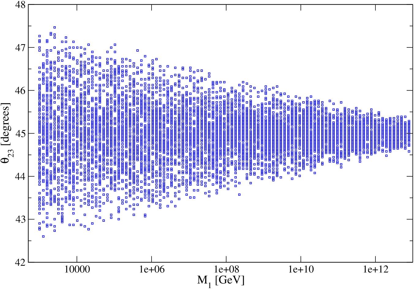
Figure 8 shows the 1-loop value of $\theta_{23}$ as a function of the lightest heavy neutrino mass. We see that it can deviate from its tree-level value by up to $2.5$ degrees and that the maximum deviation decreases with $M_{1}$. In fact, for $M_{1}\gtrsim 10^{12}$ GeV the correction is smaller than half a degree. This dependence with $M_{1}$ is very different to that observed for the matrix elements but it is consistent with it. Since the mixing angles are determined by ratios between different matrix elements, in order to have a sizable variation in the mixing angles, the structure of the neutrino mass matrix should vary significantly at 1-loop, implying that the correction should no be proportional to the identity. Hence, in models where there is a large hierarchy between the masses of the heavy neutrinos, the corrections to the mixing angles are larger. That is exactly what is observed in figure 8.

The 1-loop corrected value of $\theta_{12}$ is shown in figure 9 as a function of $M_{1}$. The variation in this case is smaller and it also decreases with $M_{1}$. More interesting for the phenomenology of neutrinos and for future experiments is the correction to $\theta_{13}$, which is exactly zero at tree level. Figure 10 shows that the 1-loop corrected value of $\theta_{13}$ can reach almost $2$ degrees, corresponding to $\sin^{2}\theta_{13}\sim 10^{-3}$, for $M_{1}$ around $1$ TeV. As expected, the maximum correction decreases with $M_{1}$, amounting to about $1$ degree ($\sin^{2}\theta_{13}\sim 3\times 10^{-4}$) for $M_{1}\sim 10^{8}$ GeV. Given that a neutrino factory could be sensitive to $\sin^{2}\theta_{13}\sim 10^{-5}$ [20], these corrections are certainly within the reach of future experiments.

The huge corrections we have found for fine-tuned models are not surprising. It is well-known in the literature that radiative corrections to fine-tuned models should spoil the tuning imposed at tree-level between the different parameters (see e.g.[21]) and that it is unnatural to expect otherwise. We have explicitly shown that that is the case. The 1-loop corrections to the neutrino mass matrix in fine-tuned seesaw models are so large that the compatibility between the tree-level seesaw formula and the experimental data becomes irrelevant. The inclusion of the 1-loop corrections is in such case necessary.

As a way of avoiding such large corrections, one may think of including the 1-loop correction into the seesaw parametrization from the very beginning. That is, one would like to look for the most general solution to equation (16) rather than to equation (9). Doing so, however, would not completely solve the problem. We would, instead, be constructing fine-tuned models at the 1-loop level, which are expected to receive large corrections at 2-loops. Fine-tuned models, it seems, are better avoided.

One possibility to do so is simply to restrict from the very beginning the magnitude of the complex angles that parametrize $\mathbf{R}$. If they are such that $\left|R_{ij}\right|_{\mbox{\tiny{max}}}\lesssim 1$ then no fine-tuning occurs and the corrections are usually under control. This additional restriction, however, has not been taken into account in previous analysis. And it was recently suggested in [18] that a fair scan of the seesaw parameter space is one in which no restriction beyond the perturbativity of the neutrino Yukawa couplings, which we have implemented, is imposed. Our results clearly demonstrate, on the contrary, that perturbativity is not enough to guarantee the stability of the neutrino mass matrix under radiative corrections and that wrong results can easily be reached if the 1-loop corrections are not taken into account. In fact, as we have seen, a significant fraction of models which are compatible with the data at tree level are no longer so once the 1-loop corrections are considered. Thus, when one is randomly scanning the parameter space of the seesaw model, it is necessary to include the finite corrections to neutrino masses.

Another possible way out is the use of a different parametrization. An alternative to the $\mathbf{R}$ parametrization that has been used in previous works is the $V_{L}$ parametrization. In it, $\mathbf{M_{D}}$ is written as

$$\mathbf{M_{D}}=\mathbf{V}_{\mathbf{R}}^{\dagger}\,\mathbf{\hat{M}_{D}}\mathbf{V_{L}}\,,$$

(23)

where $\mathbf{\hat{M}_{D}}$ is a diagonal matrix defined by the eigenvalues of $\mathbf{M_{D}}$ (real and positive) and $\mathbf{V_{L,R}}$ are unitary matrices determined by three rotation angles and three complex phases. In this parametrization, $\mathbf{\hat{M}_{D}}$, $\mathbf{V_{L}}$ and the neutrino data are used as inputs. Using equation (23) and the effective light neutrino mass matrix the following relation is obtained

$$\mathbf{\hat{M}_{D}}^{-1}\mathbf{V}_{\mathbf{L}}^{*}\mathbf{m}_{\nu}^{{\mbox{\tiny(tree)}}}\mathbf{V}_{\mathbf{L}}^{\dagger}\mathbf{\hat{M}_{D}}^{-1}=\mathbf{V_{R}^{*}}\mathbf{\hat{M}_{R}}^{-1}\mathbf{V_{R}^{\dagger}}\,,$$

(24)

which allows us to determine $\mathbf{V_{R}}$ and $\mathbf{\hat{M}_{R}}$ for a given set of input parameters. We have computed the corrections to the neutrino mass matrix also in this parametrization, and have observed that the results for $\mathbf{R}=\mathbf{I}$ and $\mathbf{R}$ real are easily reproduced for $\mathbf{V_{L}}=\mathbf{I}$ and $\mathbf{V_{L}}$ real. In particular, the large corrections for certain matrix elements are obtained there too. An important difference occurs, however, for $\mathbf{R}$ complex. Due to the different way in which the $\mathbf{V_{L}}$ parametrization samples the parameter space of the seesaw model, it is way more difficult to find fine-tuned models, with the consequence that models with very large corrections are rather scarce in the $\mathbf{V_{L}}$ parametrization.

In a future publication, we will discuss additional implications of these corrections, including their evaluation in supersymmetric scenarios as well as their possible effects in leptogenesis and lepton flavor violating processes.

The seesaw model is one of the most appealing extensions of the Standard Model that can explain neutrino masses. In this model, the mass matrix of light neutrinos receives finite corrections from 1-loop diagrams mediated by the heavy neutrinos. We considered the two different kinds of light neutrino spectra, hierarchical and inverted, and computed the corrections to the entries of the neutrino mass matrix as a function of the seesaw parameters. We found these corrections to be quite important, exceeding in several cases of interest the tree level result by orders of magnitude. Two different reasons were identified as leading to a large correction: an unusually suppressed tree-level result and an $\mathbf{R}$ matrix with elements much larger than $1$. Examples of the first case are the corrections to the matrix element ($1,3$) for NH neutrinos and to ($1,2$) and ($1,3$) for IH neutrinos. The second case can occur for $\mathbf{R}$ complex and includes the so-called fine-tuned models considered in the literature. Since these corrections can be large, models that at tree-level are compatible with the experimental neutrino data will not necessarily be so at the 1-loop level, modifying in a significant way the viable regions in the parameter space of the seesaw model. As a particular example, we studied the corrections to the mixing angles in seesaw scenarios with tribimaximal mixing and show them to lead to observable effects in future experiments. We stressed, therefore, that because of their size and importance, these corrections must necessarily be taken into account in the study and analysis of seesaw models.

We would like to thank Maria Jose Herrero, Enrico Nardi, Alejandro Ibarra and Walter Winter for useful discussions and suggestions. DAS is supported by a belgian FNRS postdoctoral fellowship. CEY is supported by DFG grant no. WI 2639/2-1.

References

- [1] Thomas Schwetz, M. A. Tortola, and Jose W. F. Valle. Three-flavour neutrino oscillation update. New J. Phys., 10:113011, 2008.
- [2] M.C. Gonzalez-Garcia, Michele Maltoni, and Jordi Salvado. Updated global fit to three neutrino mixing: status of the hints of . JHEP, 1004:056, 2010.
- [3] Peter Minkowski. at a Rate of One Out of 1-Billion Muon Decays? Phys. Lett., B67:421, 1977.
- [4] Tsutomu Yanagida. Horizontal gauge symmetry and masses of neutrinos. In Proceedings of the Workshop on the Baryon Number of the Universe and Unified Theories, Tsukuba, Japan, 13-14 Feb 1979.
- [5] Rabindra N. Mohapatra and Goran Senjanovic. Neutrino mass and spontaneous parity nonconservation. Phys. Rev. Lett., 44:912, 1980.
- [6] Murray Gell-Mann, Pierre Ramond, and Richard Slansky. COMPLEX SPINORS AND UNIFIED THEORIES. Print-80-0576 (CERN).
- [7] J. Schechter and J. W. F. Valle. Neutrino Masses in Theories. Phys. Rev., D22:2227, 1980.
- [8] J.A. Casas and A. Ibarra. Oscillating neutrinos and . Nucl.Phys., B618:171–204, 2001.
- [9] Sacha Davidson and Alejandro Ibarra. Determining seesaw parameters from weak scale measurements? JHEP, 09:013, 2001.
- [10] W. Grimus and H. Neufeld. Radiative neutrino masses in an model. Nucl. Phys., B325:18, 1989.
- [11] Apostolos Pilaftsis. Radiatively induced neutrino masses and large Higgs neutrino couplings in the standard model with Majorana fields. Z.Phys., C55:275–282, 1992.
- [12] Bernd A. Kniehl and Apostolos Pilaftsis. Mixing Renormalization in Majorana Neutrino Theories. Nucl. Phys., B474:286–308, 1996.
- [13] W. Grimus and H. Neufeld. 3-neutrino mass spectrum from combining seesaw and radiative neutrino mass mechanisms. Phys. Lett., B486:385–390, 2000.
- [14] Walter Grimus and Luis Lavoura. Softly broken lepton numbers and maximal neutrino mixing. JHEP, 07:045, 2001.
- [15] Apostolos Pilaftsis. Gauge and scheme dependence of mixing matrix renormalization. Phys. Rev., D65:115013, 2002.
- [16] Walter Grimus and Luis Lavoura. Soft lepton-flavor violation in a multi-Higgs-doublet seesaw model. Phys. Rev., D66:014016, 2002.
- [17] Walter Grimus and Luis Lavoura. One loop corrections to the seesaw mechanism in the multi-Higgs doublet standard model. Phys.Lett., B546:86–95, 2002.
- [18] J.Alberto Casas, Jesus M. Moreno, Nuria Rius, Roberto Ruiz de Austri, and Bryan Zaldivar. Fair scans of the seesaw. Consequences for predictions on LFV processes. 2010.
- [19] P. F. Harrison, D. H. Perkins, and W. G. Scott. Tri-bimaximal mixing and the neutrino oscillation data. Phys. Lett., B530:167, 2002.
- [20] Patrick Huber and Walter Winter. Neutrino factories and the ’magic’ baseline. Phys.Rev., D68:037301, 2003.
- [21] A. Ibarra, E. Molinaro, and S.T. Petcov. TeV Scale See-Saw Mechanisms of Neutrino Mass Generation, the Majorana Nature of the Heavy Singlet Neutrinos and -decay. JHEP, 1009:108, 2010.
- [22] G. Passarino and M. J. G. Veltman. One Loop Corrections for Annihilation into in the Weinberg Model. Nucl. Phys., B160:151, 1979.