Chiral symmetry breaking in QCD-like gauge theories with a confining propagator and dynamical gauge boson mass generation
Abstract
We study chiral symmetry breaking in QCD-like gauge theories introducing a confining effective propagator, as proposed recently by Cornwall, and considering the effect of dynamical gauge boson mass generation. The effective confining propagator has the form and we study the bifurcation equation finding limits on the parameter below which a satisfactory fermion mass solution is generated. Considering the evidences that the coupling constant and the gauge boson propagator are damped in the infrared, due to the presence of dynamically massive gauge bosons, the major part of the chiral breaking is mostly due to the confining propagator. We study the asymptotic behavior of the gap equation containing confinement and massive gauge boson exchange, and find that the symmetry breaking can be approximated at some extent by an effective four-fermion interaction generated by the confining propagator. We compute some QCD chiral parameters as a function of , finding values compatible with the experimental data. Within this approach we expect that lattice simulations should not see large differences between the confinement and chiral symmetry breaking scales independent of the fermionic representation and we find a simple approximate relation between the fermion condensate and dynamical mass for a given representation as a function of the parameters appearing in the effective confining propagator.
Keywords:
nonperturbative techniques , nonperturbative calculations , general properties of QCD (dynamics, confinement)1 Introduction
QCD has two main properties: the chiral symmetry breaking (CSB) and confinement of quarks and gluons. Both phenomena are related to the non-perturbative infrared (IR) dynamics. The dynamical generation of quarks masses leading to CSB can be observed through the study of QCD Green functions, what has been extensively performed in the last years by means of Schwinger-Dyson equations (SDE) [1]. Green functions can also be studied through simulations of gauge theories on the lattice, and, in particular, a great improvement in the understanding of dynamical gauge boson mass generation in these theories was obtained recently as pointed out in Ref.[2]. In what concerns gauge boson mass generation there is a nice agreement between the lattice computations and the solutions of Schwinger-Dyson equations [3, 4]. The consistency between these two different approaches, strengthened by the phenomenological consequences [5], reinforces the robust picture of gauge boson mass generation formulated by Cornwall many years ago [6, 7, 8, 9, 10, 11]. In this scenario the dynamical gluon mass induce vortices in the theory and these may be responsible for confinement.
The study of CSB through lattice simulations and the SDE approach have not come to the same firm ground as in the case of gauge boson mass generation. First, early SDE studies of CSB have shown a minute or absence of quark mass generation in the presence of dynamical gluon mass () [12, 13, 14]. Secondly, in lattice simulations it seemed that CSB and confinement were triggered by the same mechanism (at least for SU(2) theories [15, 16]). A recent result about CSB in SU(3) gauge theory indicates that we still need more simulations to confirm whether or not confinement and CSB are intimately connected, but there is a clear sign of a connection between CSB and the string tension [17]. From the point of view of gap equations we may say that something is missing in the solution of the fermionic SDE, and the most plausible possibility is confinement at least for fermions in the fundamental representation, although it may not be essential for CSB when fermions are in higher dimensional representations (e.g. “quarks" in the adjoint representation) [18]. Two recent papers tackle this problem in different ways: one introduces a confining effective propagator into the gap equation [19] and the other introduces a modified quark-gluon vertex containing information about the ghost sector as well as makes use of lattice propagators [20]. Both studies are able to explain CSB for fundamental and adjoint quarks. One of them indicate that confinement may be an essential ingredient in the gap equation [19]. The other contains a set of effects which include the use of a gluon propagator obtained from the lattice simulations and a complete vertex function that is enhanced in the infrared [20].
If CSB is a phenomena linked to confinement, as the lattice results seem to indicate, we may ask how the confinement information is embodied into the lattice gluon propagator used in the fermionic gap equation in order to generate quark masses. Anyhow, some gluon confinement effect ought to be present in the lattice propagator. However it does not show the linear confining potential felt by quarks that has also been observed in the lattice simulations [21]. The linear potential that we are referring to is the successful phenomenological quark model potential given by
| (1) |
where the confining first term is linear with the distance and proportional to the string tension . The second term, that is of order , the strong coupling constant, describes the one gluon exchange contribution. The fact that the lattice gluon propagator does not reproduce the confining part of this potential has been observed recently in Ref.[22]. The potential between static quark charges is related to the Fourier transform of the time-time component of the full gluon propagator in the following way
| (2) |
where is the Casimir eigenvalue of the fundamental representation, the bold terms, and , are 3-vectors. is the zero-zero component of the gluon propagator in the momentum configuration. As noticed in Ref.[22] the linear confining term of the potential () cannot be obtained from the gluon propagator determined in the lattice or from the gluonic SDE. Only the Fourier transform of a type of the product couplingpropagator will generate a linear term in the quark potential, although no fundamental field presents such behavior.
The proposal of Ref.[19] is attractive because it includes the necessary confining force into the gap equation, maintaining covariance and solves the problem discussed in the previous paragraph. It is a simple procedure based on critical properties of confinement and, as we will discuss, allows for a phenomenologically consistent discussion of CSB in gauge theories, providing a model that may be tested through lattice calculations. The main idea is that entropic effects, that can be associated to an area law for the Wilson quark loop, can be taken into account by a confining effective propagator of the form with a finite parameter , where is the zero-momentum value of the running quark mass and is the string tension. Using this confining effective propagator, which is to be understood as the result of a collective effect not related to the propagator of a fundamental gluon field, and responsible for quark confinement. Given this proposal within its own reasons, we aim to investigate its consequences for CSB phenomenology in the QCD case. The new gap equation is able to reproduce all QCD chiral symmetry breaking parameters.
We may say that the papers of Ref. [20] and [19] have complementary ideas and may even indicate a possible mixed picture of the CSB mechanism. In Ref. [20] it was noticed that even a quite complete treatment of the vertex function and gauge dependence of the quark SDE does not allow for CSB in agreement with experiment. A gluon propagator determined in the lattice, that is a little bit less damped in the intermediate infrared region when compared to the one obtained with the gluon SDE, is necessary, as well as some strong ghost effects into the quark-gluon vertex. However, it is not clear that introducing some complicated ghost physics into the one-gluon gap equation would lead to confining effects typical of center vortices. It is also questionable that the gluon propagators found on the lattice will be able to evidence confinement in, for example, a Wilson loop. If so much confinement is present in the one-gluon-exchange approach it would not be simple to explain how the pion ends up massless. Finally, it is not through open quark lines, as all gap equations use, that we shall observe confining effects, but through closed loops. Hence there is certain appeal on the explicit introduction of confining objects, such as center vortices. This is exactly what Cornwall’s proposal does [19], introducing an effective confining propagator whose effect is to add an extra strength to the massive gluon exchange in the infrared, with the advantage of having a simple formula to model the IR QCD behavior. We also recall that it has been argued that the one-gluon massive exchange and the confining gluon propagators act differently when quarks are in the fundamental and adjoint representations [18], therefore we have a precise way to investigate the possible differences in the CSB and confinement transitions for fermions in different representations. We will argue that CSB is a direct consequence of confinement in this specific model.
The article is organized as follows. In Sect. II, we describe briefly the model of Ref.[19], i.e. how confinement is introduced in the gap equation. In Sect. III, we study the bifurcation equation of the full gap equation. It is verified that we have maximum values in order to generate reasonable values for the dynamical quark mass. In Sect. IV, we present an analysis of the asymptotic behavior of the gap equation. The idea was to investigate how confinement could affect the asymptotic behavior of the fermionic self-energy. It must be said that the CSB mechanism is not only important for QCD, but for any non-Abelian gauge theory. In particular, it has consequences for the Standard Model dynamical gauge symmetry breaking, or the so called Technicolor models. We find that if the confinement effective propagator were restricted to a limited region of momenta the self-energy is well approximated by an effective four-fermion interaction. In Sect. V we compute quantities like the pion decay constant and the quark condensate verifying that the model predicts reasonable values for the QCD chiral parameters. In Sect. VI we determine an approximate relation between the fermion condensate and the dynamical mass for a given representation as a function of the parameters appearing in the confining effective propagator. These quantities can be studied through lattice simulations and may provide a test for this CSB mechanism. In Sect. VII, we draw our conclusions.
2 Introducing confinement into the gap equation
The possible relation between confinement and chiral symmetry breaking for quarks in the fundamental representation is an issue discussed several times in the literature in many different contexts as pointed out in Ref.[18]. With the evidence that gluons acquire a dynamically generated mass [2, 3, 4], i.e. a momentum dependent mass , it also becomes clear that the standard quark gap equation with dynamically massive gluons does not have enough strength to generate quark masses. Therefore, if CSB and confinement are triggered by the same mechanism, the main quest in this subject is how to introduce confinement into the quark SDE.
The proposal of Ref.[19] is that confinement should be introduced into the gap equation through the following effective propagator, meaning that it is not at all related to the propagation of a standard quantum field:
| (3) |
In the limit we obtain the standard effective propagator , that yields approximately an area law for the Wilson loop. We must necessarily have a finite value due to entropic reasons as demonstrated in Ref.[19], and it is related to the dynamical quark mass, as required by gauge invariance. Moreover, the Abelian gauge invariance of this effective propagator must appear in the quark action obtained by integrating over quark world lines that will imply a area-law action [19]. With the inverse fermionic propagator written as
using the approximation , which implies that turns out to be identical to the dynamical mass , we can see that the effective propagator of Eq.(3) leads to an Abelian gluon gap equation equal to
| (4) |
where is the running dynamical quark mass generated by the confining propagator, so we end up with
| (5) |
Note that there is an interplay between the parameters , and as extensively discussed in Ref.[19], and we will comment about their values, but it must be said that they should be related among themselves because in the end all of them will be proportional to the QCD mass scale .
Eq.(5) is not the whole story, since it was also recognized that massive one-dressed-gluon exchange may induce a quite small CSB for fermions in the fundamental representation as well as a larger symmetry breaking for fermions in higher dimensional representations [18, 20], which, in the Landau gauge, is given by
| (6) |
where is the quark Casimir eigenvalue and is the effective charge
| (7) |
where for the group with flavors. For quarks in the fundamental representation and with the phenomenologically preferred value MeV [5], we see that this charge’s value at the infrared fixed point [25, 26] () is of order , as shown in Fig.(1), while it should be at least a factor larger to trigger CSB.

For “quarks" in the adjoint representation the Casimir eigenvalue is approximately a factor two larger and compensates the small effective coupling [18, 20]. The ultimate gap equation may be quite sophisticated but it can be well modeled by the sum of the “confining" plus massive one-gluon exchange [19], which, in the Abelian gluon approximation, is given by
| (8) | |||||
where is the dynamical quark mass generated by the confining and one-dressed-gluon propagators. This last equation is the basic one that we shall explore in this work. We could say that this equation resembles, in a different context, what we have in the phenomenological quark model potential described in Eq.(1), i.e. a part that is responsible by confinement (generating an approximately linear term proportional to the string tension), and the second term, that is of order , describing the one-gluon exchange contribution. Thereof, confining part of Eq.(8) is a reasonable phenomenological way to study CSB taking into account the effective area law.
The solution of the confining gap equation (Eq.(5)) was discussed by Cornwall [19], and it was observed that the confining propagator generates CSB represented by a dynamical quark mass that is of order . This dynamical quark mass has a fast large momentum falloff (), which results from a gap equation basically dominated by the infrared region of the propagator. On the other hand the -gluon gap equation was extensively studied in the literature and it is known that it generates CSB only above a certain critical coupling equal to , which, as discussed in the previous paragraph, is not achieved by the effective coupling of Eq.(7). Notice that the suggestion of a hypothetical Casimir scaling law for CSB with fermions in the representation [23, 24]
| (9) |
appears as a consequence of the SDE equation without the existence of a dynamical gauge boson mass.
It is easy to verify that Eq.(5) has nontrivial solutions. Its critical behavior can be inferred from the derivative of Eq.(6) with respect to , where we can replace by (in the constant coupling limit), linearize with the substitution of in the denominator by , and evaluate at :
| (10) |
Eq.(6) has already been solved with different approximations [12, 13, 19], and has solutions only for large values as noticed in Ref.[19]. The condition for Eq.(10) to have a nontrivial solution (and consequently Eq.(5)) is the same one that Eq.(6) has to obey. Considering the damped confining propagator that leads to an effective coupling (that is now in the place of ), and the fact that [19], we verify, just by transposing the results of Ref.[12, 13, 19, 27, 28] (see, particularly, the simple analysis shown in section 3 of Ref.[13]), that chiral symmetry will always be broken with the confining propagator. Therefore, the above procedure leads to the solutions of Eq.(5) that can be represented by a linear combination of the following expressions:
| (11) |
obtained from the derivative of the solutions of Eq.(6), where is the step function and
The value of is determined by the boundary condition at
| (12) |
It seems that the confining effective propagator for the and values discussed above is able to describe the chiral symmetry breaking. However the full CSB problem, as discussed by Cornwall [19], includes the effect of the dressed -gluon exchange, and the critical behavior for the onset of dynamical quark masses in this case will be discussed in the next section. It is possible that only the sum of these effects may explain the lattice results for CSB [17].
3 Critical behavior of the complete gap equation
We can discover some aspects about Eq.(8) critical behavior examining its bifurcation equation. To verify at what point the nontrivial solution of Eq.(8) bifurcates away from trivial solution, it is sufficient to consider the linearized version of that equation [27, 28]. We will deviate from the standard bifurcation theory proceeding as in Ref.[29], and instead of substituting by in the denominators of Eq.(8), we will replace this term by and define the IR value of the dynamical quark mass () by the normalization condition
following these steps we arrive at our bifurcation equation
| (13) | |||||
Our main intention in this section is to verify the gross critical behavior of the gap equation with these infrared finite propagators, this is the reason to select a bare massive gluon in Eq.(13). This equation is a standard Fredholm equation with a positive kernel, and, requiring to belong to , the spectrum is discrete with a smallest value for the “effective coupling" and the -gluon exchange coupling such that we have the trivial solution for values of these couplings smaller than a certain critical value, and the nontrivial one if their values are larger than this same critical value.
We can still make some simplifier approximations before estimating the critical behavior of Eq.(13), making the following substitutions
| (14) |
and
| (15) |
which is known as the angle approximation, and introduces an error of about in the calculation [30]. If we also define the variables , , , , and , we obtain
| (16) |
where we introduced an ultraviolet cutoff () and the kernel is equal to
| (17) | |||||
The kernel is square integrable
| (18) | |||||
therefore Eq.(16) has a nontrivial solution for its coupling on a point set. The smallest eigenvalue (which, as we shall see, is related to the value of ) for which Eq.(16) has a nontrivial square integrable solution, is the first bifurcation of the nonlinear equation, and satisfies
| (19) |
Note that the kernel contains the sum of two contributions, that we may denote and , corresponding to the confining and dressed -gluon exchange propagator. From the triangle inequality we know that
| (20) |
from which we can recover the early results for the -gluon exchange, i.e. if the gluon mass is not introduced into the gap equation and the confining propagator is neglected, the limit of Eq.(19) is obtained only due to the contribution with a critical coupling constant , but the contribution is necessary when considering dynamically massive gluons and quarks in the fundamental representation.

The bifurcation condition described by Eq.(19) is depicted in Fig.(2) in the case of , MeV and GeV2, where it is shown a dashed (blue) curve obtained with MeV, a dot-dashed (red) curve with MeV and a solid (black) curve with MeV. Each point of these curves indicate the bifurcation point for a given value generating a dynamical quark mass . It should be noticed that there is a maximum value above which there is no CSB, and this maximum value does not vary much as we change the values of the dynamical gluon mass. It is also interesting to verify that CSB also receives contributions from the massive gluon term, and this is the reason for the differences between the curves, though the massive gluon (or -gluon exchange) generates a minute mass, as already observed many years ago in Ref.[12, 13]. As the dynamical gluon mass is decreased we can observe a small increase in the maximum value of the parameter, due to the -gluon exchange increasing contribution to the gap equation. When the bifurcation condition is computed it is possible to verify a larger instability in the numerical procedure as we go to larger values of and (for large values), which is due to the fact that we have two contributions to the chiral breaking, but with one of the kernels contributing much more to the breaking than the other. This fact is obvious if we compare the different propagators that we are dealing with. These propagators are shown in Fig.(3) and Fig(4) for typical mass parameters that we are discussing in this work. We can see a huge difference between the two propagators (). Of course, the confining effective propagator should not be regarded as the actual gluon propagator, but must be seen as a collective effect that produces confinement, with an area law for the quark action and appropriate entropic properties [19]. The difference between these contributions are responsible for the delicate convergence of the bifurcation condition.
It must be also noticed that the confining effective propagator has most of its effect concentrated in a momentum region below MeV. Actually, as we shall discuss ahead, most of the chiral symmetry breaking will occur due to the low momentum region of the gap equation, what is consistent with lattice observations that the relevant momentum component of gluons for CSB is exactly this region [31, 32, 33]. This fact may be contrasted with the results of Ref.[20], where a larger part of the CSB comes from an intermediate region of GeV.


4 The asymptotic behavior of the gap equation
The asymptotic behavior of the complete gap equation [Eq.(8)] can be obtained from the linearized Eq.(16) with the kernel given by Eq.(17) in a procedure identical to the one performed by Takeuchi [34] and Kondo, Shuto and Yamawaki [35]. In these references the QCD CSB problem was solved considering a quark Schwinger-Dyson equation also with a two kernel contribution: One due to an effective four-fermion interaction and another one due to a perturbative gluon exchange.
The integral equation (16) with the kernel described in Eq.(17) can be transformed into a differential equation and solved with appropriate boundary conditions. In order to still simplify the calculation we assume
| (21) |
and neglect the running of the coupling constant in Eq.(17). The fact that we consider all masses equal to , as implied by Eq.(21), shall not modify the asymptotic behavior of the quark self-energy, and the assumption of a constant coupling will introduce sub-leading or logarithmic corrections to the asymptotic solution. After these approximations we obtain the following differential equation
| (22) | |||||
where
| (23) |
with the infrared and ultraviolet boundary conditions given respectively by
| (24) |
The asymptotic solution of the linear second-order differential equation, with a singularity at infinity, is obtained as a linear combination of two independent solutions, , which can be obtained by applying the expansion method [36]. Eq.(22) can be put in the form , where and can be expanded in convergent series of the form and for large . The asymptotic solutions are of the form
| (25) |
where are the roots of
| (26) |
With the leading coefficients of the differential equation given by and we obtain two roots
| (27) |
Defining a new variable
| (28) |
we can write the asymptotic solution as
| (29) |
The substitution of Eq.(25), with given by Eq.(28), into the differential equation (22) allows the determination of the coefficients and the recursion formula satisfied by them.
Considering only the “" solution displayed in Eq.(29), with the definitions
| (30) |
we obtain the following recursion formula
| (31) |
and verify, for example, that the first two coefficients of the “" series are related by
| (32) |
For the “" solution we just have to exchange for and for in Eqs.(30) to (32). If we keep only the leading terms in we can write and . Applying the UV boundary condition we obtain that
| (33) |
The IR boundary conditions force the solutions to be equal to as , and the amount each solution ( or ) contributes to the self-energy can be measured by the ratio
| (34) |
The ratio indicates which solution dominates the CSB. To gain some insight on the problem we can recall that when the gluons are massive the coupling constant (see Eq.(7)) is not expected to be larger than , therefore is a small number, and we can see that in the limit , the coefficients and are large and , leading us to and , implying
| (35) |
In the ultraviolet limit we verify that the ratio behaves as and the solution gives the asymptotic behavior of the self-energy. This is, apart from logarithmic contributions, the known behavior found by Politzer using the operator product expansion [37]. Notice that the asymptotic behavior is fully described by the -gluon exchange, and this is not much different from what was found by Takeuchi [34] in a problem where the CSB is dominated by a four-fermion interaction. The influence of the confining propagator enters only through the boundary conditions. As the mass solution that comes from the confining contribution has a fast falloff, almost behaving as an effective four-fermion interaction it is not surprising at all to see the similarity of our Eq.(35) to Eq.(29) of Ref.[34]. Another interesting limit of Eq.(35) is obtained when , or , although this may happen only for almost conformal theories, and it is a case of interest for technicolor models. We mention this because has an upper limit when the gauge bosons acquire a dynamically generated mass, as shown in Eq.(7) [38], and consequently we must force the function coefficient in Eq.(7) to be very small in order to have , and it may be quite difficult to build realistic technicolor theories with . This particular possibility is under study and will be presented elsewhere.
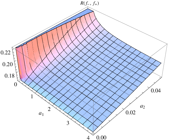
Equation (35) would have a different (and interesting) behavior if the upper cutoff () were of order . This would happen if the integration of the confining part of the gap equation, the one responsible for the CSB, were limited to a region in momentum smaller than, or of the order of the scale . Assuming an upper limit in the momentum integration, we show in Fig.(5) the ratio when as a function of and . This ratio is smaller than indicating that the asymptotic behavior of the irregular symmetry breaking solution would dominate over the regular one in this particular limit. In order to explore even more this possibility we can assume that the confining contribution could be reduced to an effective four-fermion interaction. Some of the reasons why we are concerned with the possibility of generating a four-fermion interaction are the following: First, if confinement is introduced into the gap equation we should expect to reproduce some of the many phenomenological successful quark-models based on the Nambu-Jona-Lasinio type of interaction. Secondly, lattice simulations show that the relevant gluonic energy scale of spontaneous CSB is due to the low-momentum component of the gluon field [31, 32, 33], which may indicate the possibility of a natural upper cutoff in the momentum. The existence of a specific momentum that separates the confinement and perturbative regions has also been discussed in a different context [39]. Finally, the existence of a completely nonperturbative infrared fixed point, as happens when the theory develops a dynamical gauge boson mass [25], may induce effective four-fermion interactions as discussed many years ago in Ref.[40, 41].
It is known that as long as we have a “massive" gluon propagator it would be possible to consider that this mass could be factorized from the propagator generating an effective four-fermion interaction, but this is not true because the actual interaction strength is measured by the product “couplingpropagator", and we know from Eq.(7) that the -gluon exchange has not strength enough to generate such effective coupling. On the other hand the confining effective propagator, with the usual values for the string tension, is strong enough to generate the following effective gap equation:
| (36) | |||||
Apart from the gluon mass effect appearing in the -gluon contribution, the above equation has been extensively studied in Refs. [34] and [35], and it does lead to a self-energy solution that decreases slowly with the momentum, or the so called irregular solution for the self-energy [35]. The solution of Eq.(36) follows from Refs. [34] and [35] observing the interplay between their -fermion coupling constant and our effective coupling .
The critical behavior of Eq.(36) can be compared to the one of the complete Eq.(16) studied in the previous section, but now with a -fermion effective kernel given by
| (37) | |||||
We separated the kernel of Eq.(37) into two different kernels, one due to the effective four-fermion interaction and another due to the exchange of a massive gluon. Using the triangle inequality of Eq.(20) and the bifurcation condition given by Eq.(19) we compute the critical condition and show in Fig.(6) the dot-dashed (black) curve of critical values for the generation of massive solutions of Eq.(36). This curve was obtained for MeV, , MeV and GeV2, and for comparison we also draw in Fig.(6) the dashed (blue) critical curve of the complete kernel given by Eq.(17) (without the four-fermion approximation) computed with the same parameters. This shows that most of the symmetry breaking is driven by the confining effective propagator and the four-fermion approximation is reasonable up to an order of . Since we simplified the gap equation and used the triangle inequality to obtain the curve of Fig.(6), it is difficult to say how much of the difference between these curves result from the numerical procedure. However it indicates that the confinement effect, as proposed in Ref.[19], may indeed be the generator of an effective four-fermion interaction.

We also computed the bifurcation condition (Eq.(19)) with the part only due to the confining kernel in the four-fermion approximation for different values of the string tension. The result is shown in Fig.(7) where the continuous (blue) curve was obtained for GeV2 and the dot-dashed (black) and dashed (blue) were obtained respectively for and GeV2. Small changes in the string tension introduce larger effects than the ones that can be observed when we vary the gauge boson mass in the bifurcation case of the complete gap equation. This confirms again the dominance of the confining effective propagator.
There is no doubt that the confining gap equation can be reduced to an effective four-fermion approximation. However we would like to claim that the confining part of the fermionic SDE should have an upper cutoff at some scale not too much different from . The reason for this is that the linear potential must break at some critical distance. For quarks in the fundamental representation, lattice QCD data shows that the string breaks at the following critical distance [42]
| (38) |
which corresponds to a value compatible with the one necessary for the expected amount of CSB.

The results obtained up to now contain many approximations, as the assumption that all mass scales were the same. A realistic calculation taking into account the different mass scales that we have in the original equation will be performed numerically in the next section, however we may see that the effect of the confining propagator dominates over the -gluon exchange and may even modify the asymptotic behavior of the gap equation as seen in the four-fermion approximation, which retains the CSB information.
5 Chiral parameters with confinement and massive gluons
In the above sections we studied aspects of the bifurcation equation as well as the asymptotic behavior of the full gap equation, but to know how the proposal of Ref.[19] provides the right amount of chiral symmetry breaking it is necessary a full computation of the complete gap equation without the approximations made above or in Ref.[19]. We now solve Eq.(8) without the angle approximation and taking into account the running coupling constant, with its infrared value dictated by a dynamical gluon mass, and a massive gluon propagator with the running mass included exactly as determined in the Ref.[6]. We choose the same values of , , and that were used to obtain Fig.(2), but select an infrared value of the dynamical gluon mass equal to MeV, which is an average of many determinations of this parameter [5]. We compute numerically the full gap equation for the dynamical quark mass with different values and show the results in Fig.(8).

A reasonable dynamical quark mass of MeV is obtained with a value equal to MeV. This is a little smaller but totally consistent, within the different approximations, to the one obtained in Ref. [19].
In order to show how reasonable the four-fermion approximation is to the complete gap equation we plot in Fig.(9) the numerical calculation of Eq.(36). This figure was obtained with MeV, , MeV, GeV2 and MeV. The infrared value of the dynamical quark mass is overestimated by an compared to the one of Fig.(8), while it is also evident the slowly decreasing behavior of the dynamical fermion mass with the momentum as it was advanced in the previous section. The fact that the four-fermion approximation overestimates the dynamical quark mass was already observed in Fig.(6).

To confirm that the scenario of Ref. [19] is fully consistent with the CSB phenomenology, we compute several chiral parameters with the same values of , , and discussed above and MeV, which leads to the usually expected dynamical quark mass of MeV. The chiral parameters, computed in the Abelian gluon approximation, that we consider are:
| (39) |
There are many improvements to this formula, one of them determined in Ref.[45], which gives the following correction factor
| (40) |
and the pion decay constant is obtained as the result of the sum
| (41) |
which is to be compared to the experimental value MeV [46].
b) The quark condensate at the scale GeV2 [1]
| (42) |
which should be compared to typical value of the quark condensate ( GeV2) MeV3 [47].
c) The MIT bag constant B [48]
The results for the three parameters discussed above, computed as a function of , are shown in Table (1). Considering the simple rainbow approximation for the gap equation we see that the results are below the expected values, but better choices for the vertex function as well as higher order corrections for these quantities will bring them closer to the experimental values.
160 62.0 71.12 169.03 100.09 180 54.51 61.83 156.12 84.96 200 46.59 52.14 142.0 69.43 Expected Values 93 93 146
6 CSB for higher dimensional representations
The study of CSB for fermions in higher dimensional representations is of interest because it is a possible way to verify how this mechanism is distinct from the confinement one, as well as it is important for technicolor model building. If a type of Casimir scaling as the one predicted by Eq.(9) occurs, we expect that for higher dimensional representations the CSB typical mass scale would be different from the one for the fundamental representation, and perhaps different from the confinement scale. It has also been argued that for “quarks" in the adjoint representation the dynamically massive gluons may have enough strength to generate a dynamical quark mass [18, 20]. Indeed in Ref.[20] a large dynamical mass was found for fermions in the adjoint representation, and we naively would expect that in this case the confining and chiral breaking transitions would appear separately.
If we follow straightforwardly the model of Ref.[19] we must also verify what is the difference introduced by the confining propagator in the case of higher dimensional representations, because in principle we should replace the string tension by , which is the string tension for fermions in the representation . We assume that this replacement is accurate, although we know that the phenomenological potential of Eq.(1), and consequently the string tension, does change according to the representation. For instance, in the case of the adjoint representation it is known that
| (44) |
where is the energy of the lightest glueball. Moreover, the adjoint representation is not confined but screened [21], what means that the confining propagator should be understood as effective up to a certain distance in these cases. Of course, no matter what the fermionic representation is we shall have a critical distance above which the string breaks. We assume that in the model of Ref.[19] most of the chiral symmetry breaking is still related to the form of Eq.(3), which does not get the chance to be probed at large distances, consequently we may still expect that most of the CSB is driven by the “confining" propagator.
The fermion condensate is the most frequent quantity used to characterize the chiral phase transition, and it is this quantity that we will analyze to investigate CSB for fermions in different representations. The fermion condensate is described by Eq.(42). It is easy to compute this quantity for different fermion representations if we consider the gap equation in the four-fermion approximation given by Eq.(36), perform the angle approximation and neglect the gauge boson mass in the propagator of the -gauge boson exchange contribution:
| (45) | |||||
On the other hand we may write the fermion condensate for the representation in the following form
| (46) |
where is the dimension of the fermion representation and its dynamical mass. We are forcing the upper limit of Eq.(46) to be of , which can be as low as GeV, while is well known at the GeV scale. We did this, as we shall see below, in order to easily compare the condensate expression to Eq.(45), but we can check that Eq.(46) provides a good estimate of the quark condensate at GeV. To do so we see that in the four-fermion approximation the dynamical quark mass is almost flat up to GeV, as can be seen in Fig.(9), and its value is around , therefore the integral in Eq.(46) can be approximated by . With for the fundamental representation we obtain GeV3, which is a little large but consistent with the fact that the four-fermion approximation overestimates the dynamical mass. We stress that the upper limit in the first integral in the right-hand side of Eq.(45) may be a physical one in order to be consistent with the critical distance at which the string breaks, as shown in Eq.(38).
Eq.(46) can be compared to Eq.(45), the dynamical fermion mass in the four-fermion approximation, if we set all integrals at the scale obtaining
| (47) |
Since the first term between brackets in the right-hand side of Eq.(47) is much larger than the second one, combining the two last equations we have
| (48) |
In the QCD case, for quarks in the fundamental representation, this relation underestimates the condensate due to the fact that the integration area in this equation was drastically reduced when we cutoff the integral at , whereas the dynamical quark mass solution, as shown in Fig.(9), is almost flat up to GeV2. Since the effect of the Eq.(3) is the dominating one, it is quite plausible that the relation of Eq.(48) holds up to other scales (still keeping the factor in the right-hand side) and it can be tested through lattice simulations.
We can now make a few comments on the differences between CSB for fermions in the fundamental and adjoint representations estimating the ratio of the condensates for fermions in these representations. First we need to know how the string tension changes as we change the fermion representation. It has been observed in lattice simulations what is usually called Casimir scaling for the string tension [21], i.e.
| (49) |
where is the ratio between the Casimir operators for the representation and the fundamental one. For theories and a finite the Casimir scaling law must break down at some point, to be replaced by a dependence on the -ality of the representation [21]
| (50) |
This change of behavior is credited to an effect of force screening by the gauge bosons. For fermions in the adjoint representation the -ality is zero, therefore, according to Casimir scaling, the adjoint string tension is given by
| (51) |
and, as a reasonable approximation, we may assume . Consequently we obtain the following ratio at the scale
| (52) |
Once the dynamical masses almost scale with the string tension value we could say that the above ratio is roughly of order . Of course, the uncertainty in this estimative is certainly connected to the remarks made at the beginning of this section about the phenomenological potential and the effective propagator for the adjoint representation. For other fermionic representations the screening behavior is smaller, although in all cases we certainly have a limit on the critical distance for which this approach is valid that will be connected with the string breaking mechanism.
7 Conclusions
In this work chiral symmetry breaking for QCD-like theories was studied in the case of a rainbow Schwinger-Dyson equation in the presence of dynamically massive gauge bosons. Confinement was also introduced into the SDE in the form of an effective propagator which is one that can reproduce an area law for quarks. This is a phenomenological way to investigate the possibility, indicated by the lattice, of confinement (by center vortices) being intrinsically related to chiral symmetry breaking.
We briefly review the conditions for the confining propagator to generate non-trivial massive solutions. We studied the bifurcation condition for the complete gap equation, i.e. the one with the exchange of dynamically massive gauge bosons and with the inclusion of the confining effective propagator dependent on the entropic parameter , which must be proportional to the dynamical quark mass, and on the string tension , verifying that there is a maximum value below which the chiral symmetry is broken, and generating the expected values for the dynamical quark masses. As already known in the literature we verified that the massive gauge boson exchange gives only a minute contribution to the dynamical fermion mass. Most of the breaking is due to the confining propagator and this may be one indication that we should not expect large differences between the chiral and confinement transitions.
The asymptotic behavior of the gap equation was studied in order to evaluate how confinement may affect the asymptotic self-energy. We observed that if the confining effect is restricted to a small momentum region, presenting some arguments for why this may happen, the solution changes its behavior from the one obtained with the help of the operator product expansion to a self-energy typical of a four-fermion interaction. It is known that the massive gauge boson gap equation cannot be reduced to an effective four-fermion interaction due to the small infrared strength of the product “couplingpropagator", however we verified that this is not the case for the confining effective propagator. The bifurcation equation for the gap equation with the four-fermion approximation performed in the confining part reproduces approximately the result of the complete gap equation without any approximation. Actually this approximation overestimates the dynamically generated fermion mass by an .
The complete gap equation was computed numerically without any approximation in Section V. Our result for the dynamical fermion mass is consistent with the one obtained by Cornwall [19]. We also computed several chiral parameters which resulted to be of the order of the expected experimental values. These parameters show dependence on the effective propagator scale , however larger differences in the dynamical mass can also be observed with a small variation of the string tension value (see Fig.(7)).
In Section VI we discuss the case of chiral symmetry breaking for fermionic representations different than the fundamental one. We found a simple relation between the fermion condensate and the fermionic dynamical mass. This relation depends on the dimension of the fermion representation, and , and we assumed that the form of Eq.(3) still holds for different fermionic representations up to a certain distance. In principle such relation can be studied in lattice simulations. Since most of the symmetry breaking is due to the confining effective propagator and the string tension approximately scales with the Casimir operator, we do expect simple relations between the condensate values for different representations, but no matter what representation we choose it seems that in this scenario we shall not have large differences between the confining and chiral transition mass scales.
Our results indicate that the CSB mechanism proposed in Ref.[19] can account for the expected values of several
known chiral parameters. The model also seems to indicate that the CSB scale is connected to the confinement one even
for fermions in higher dimensional representations.
How far can we assume the four-fermion approximation discussed here for the purpose of practical
calculations still needs further analysis. Finally, a more precise determination of the CSB observables can be obtained with
the introduction of more sophisticated vertex functions and higher order corrections.
Acknowledgments
We are indebted to A. C. Aguilar for discussions and help with the numerical calculation and are grateful to Prof. J. M. Cornwall for a clarifying exchange of correspondence and comments on a previous version of this manuscript. This research was partially supported by the Conselho Nacional de Desenvolvimento Científico e Tecnológico (CNPq) (AD and AAN), and Fundação de Amparo a Pesquisa do Estado de São Paulo (FAPESP) (FAM).
References
- [1] C. D. Roberts and A. G. Williams, Prog. Part. Nucl. Phys. 33, 477 (1994).
- [2] A. Cucchieri and T. Mendes, PoS QCD-TNT 09, 026 (2009).
- [3] A. C. Aguilar, D. Binosi and J. Papavassiliou, Phys. Rev. D 78, 025010 2008.
- [4] A. C. Aguilar, D. Binosi and J. Papavassiliou, Phys. Rev. D 81, 125025 (2010).
- [5] A. A. Natale, PoS QCD-TNT 09, 031 (2009).
- [6] J. M. Cornwall, Phys. Rev. D 26, 1453 (1982).
- [7] A. C. Aguilar and J. Papavassiliou, JHEP 0612, 012 (2006).
- [8] A. C. Aguilar and J. Papavassiliou, Eur. Phys. J. A 35, 189 (2008).
- [9] A. C. Aguilar and J. Papavassiliou, Phys. Rev. D 81, 034003 (2010).
- [10] D. Binosi and J. Papavassiliou, JHEP 0811, 063 (2008).
- [11] D. Binosi and J. Papavassiliou, Phys. Rept. 479, 1 (2009).
- [12] B. Haeri and M. B. Haeri, Phys. Rev. D 43, 3732 (1991).
- [13] A. A. Natale and P. S. Rodrigues da Silva, Phys. Lett. B 392, 444 (1997).
- [14] A. A. Natale and P. S. Rodrigues da Silva, Phys. Lett. B 390, 378 (1997).
- [15] P. O. Bowman, et al., Phys. Rev. D 78, 054509 (2008).
- [16] R. Hollwieser, M. Faber, J. Greensite, U. M. Heller and S. Olejnik, Phys. Rev. D 78, 054508 (2008).
- [17] P. O. Bowman, et al., Phys. Rev. D 84, 034501 (2011).
- [18] J. M. Cornwall, Invited talk at the conference “Approaches to Quantum Chromodynamics", Oberwölz, Austria, September 2008, hep-ph/0812.0359.
- [19] J. M. Cornwall, Phys. Rev. D 83, 076001 (2011).
- [20] A. C. Aguilar and J. Papavassiliou, Phys. Rev. D 83, 014013 (2011).
- [21] J. Greensite, Prog. Part. Nucl. Phys. 51, 1 (2003).
- [22] P. Gonzalez, V. Mathieu and V. Vento, hep-ph/1108.2347.
- [23] W. J. Marciano, Phys. Rev. D 21, 2425 (1980).
- [24] S. Raby, S. Dimopoulos and L. Susskind, Nucl. Phys. B 169, 373 (1980).
- [25] A. C. Aguilar, A. A. Natale and P. S. Rodrigues da Silva, Phys. Rev. Lett. 90, 152001 (2003);
- [26] A. C. Aguilar, A. Mihara and A. A. Natale, Phys. Rev. D 65, 054011 (2002).
- [27] D. Atkinson, J. Math. Phys. 28, 2494 (1987).
- [28] D. Atkinson and P. W. Johnson, Phys. Rev. D 35, 1943 (1987).
- [29] D. Atkinson, V. P. Gusynin and P. Maris, Phys. Lett. B 303, 157 (1993).
- [30] C. D. Roberts and B. H. J. McKellar, Phys. Rev. D 41, 672 (1990).
- [31] A. Yamamoto and H. Suganuma , Phys. Rev. D 81, 014506 (2010).
- [32] A. Yamamoto and H. Suganuma, PoS Lattice 2010, 294 (2010), hep-lat/1008.1624;
- [33] H. Suganuma, et al., hep-lat/1103.4015.
- [34] T. Takeuchi, Phys. Rev. D 40, 2697 (1989).
- [35] K.-I. Kondo, S. Shuto and K. Yamawaki, Mod. Phys. Lett. A 6, 3385 (1991).
- [36] F. W. J. Olver, Asymptotics and special functions, Academic Press, (1974).
- [37] H. D. Politzer, Nucl. Phys. B 117, 397 (1976).
- [38] J. M. Cornwall, Phys. Rev. D 80, 096001 (2009).
- [39] S. J. Brodsky and R. Shrock, Phys. Lett. B 666, 95 (2008).
- [40] W. A. Bardeen, C. N. Leung and S. T. Love, Phys. Rev. Lett. 56, 1230 (1986).
- [41] W. A. Bardeen, C. N. Leung and S. T. Love, Nucl. Phys. B 273, 649 (1986)
- [42] G. S. Bali et al. [SESAM Collaboration], Phys. Rev. D 71, 114513 (2005).
- [43] H. Pagels and S. Stokar, Phys. Rev. D 20, 2947 (1979).
- [44] J. M. Cornwall, Phys. Rev. D 22, 1452 (1980).
- [45] A. Barducci, R. Casalbuoni, M. Modugno, G. Pettini and R. Gatto, Phys. Lett. B 405, 173 (1997).
- [46] K. Nakamura et al. [Particle Data Group], J. Phys. G 37, 075021 (2010).
- [47] V. Gimenez, V.Lubicz, F. Mescia, V. Porretti and J. Reyes, Eur. Phys. J. C 41, 535 (2005) and references therein.
- [48] R. T. Cahill and C. D. Roberts, Phys. Rev. D 32, 2419 (1985).
- [49] A. Chodos, R. L. Jaffe, K. Johnson, C. B. Thorn and V. F. Weisskopf, Phys. Rev. D 9, 3471 (1974).
- [50] A. Chodos, R. L. Jaffe, K. Johnson and C. B. Thorn, Phys. Rev. D 10, 2599 (1974).
- [51] T. De Grand, R. L. Jaffe, K. Johnson and J. Kiskis, Phys. Rev. D 12, 2060 (1975).