Optimal Dividend Policies for Piecewise-Deterministic Compound Poisson Risk ModelsThanks: This research was supported in part by National Science Foundation under grant DMS-1108782 and from the UWM Research Growth Initiative, and City University of Hong Kong (SRG) 7002677.

Runhuan Feng University of Illinois at Urbana-Champaign Affiliation: Hans W. Volkmer, University of Wisconsin - Milwaukee Affiliation: Shuaiqi Zhang, Hebei University of Technology Affiliation: Chao Zhu, University of Wisconsin - Milwaukee

Abstract

This paper considers the optimal dividend payment problem in piecewise-deterministic compound Poisson risk models. The objective is to maximize the expected discounted dividend payout up to the time of ruin. We provide a comparative study in this general framework of both restricted and unrestricted payment schemes, which were only previously treated separately in certain special cases of risk models in the literature. In the case of restricted payment scheme, the value function is shown to be a classical solution of the corresponding HJB equation, which in turn leads to an optimal restricted payment policy known as the threshold strategy. In the case of unrestricted payment scheme, by solving the associated integro-differential quasi-variational inequality, we obtain the value function as well as an optimal unrestricted dividend payment scheme known as the barrier strategy. When claim sizes are exponentially distributed, we provide easily verifiable conditions under which the threshold and barrier strategies are optimal restricted and unrestricted dividend payment policies, respectively. The main results are illustrated with several examples, including a new example concerning regressive growth rates.

Key Words. Piecewise-deterministic compound Poisson model, HJB equation, quasi-variational inequality, threshold strategy, barrier strategy.

AMS subject classifications. 93E20, 60J75

1 Introduction

The dividend problem in classical insurance risk models was originated in de Finetti, (1957), and drew revived interests in recent literature focusing on optimization of dividend payment strategies. The optimality is often considered to be a strategy which maximizes the expected present value of dividends received by the shareholders. Jeanblanc-Picqué and Shiryaev, (1995) and Asmussen and Taksar, (1997) investigated in diffusion models the dividend problems where the dividends are permitted to be paid out up to a maximal constant rate or a ceiling. We shall refer to such a type of dividend problem as restricted payment scheme. It was shown in their papers that the dividends should be paid out at the maximal admissible rate as soon as the surplus exceeds a certain threshold. Interestingly, it turns out that such a threshold strategy is the optimal restricted payment scheme in a variety of other risk models. For example, Gerber and Shiu, (2006) discussed the threshold strategy in the compound Poisson model and solved the problem explicitly when the claim size is exponentially distributed. Fang and Wu, (2007) studied a similar problem in the compound Poisson risk model with constant interest and showed the optimal dividend strategy is a threshold strategy for the case of an exponential claim distribution. See also Asmussen et al., (2000), Bai and Paulsen, (2010), Choulli et al., (2003), Hunting and Paulsen, (2013) Schmidli, (2002), and references therein for some important developments on optimal dividend policies in the setting of controlled diffusions.

On the other hand, there was also a significant amount of literature in which no such restriction of maximal rate is imposed on dividend payment strategies. We shall refer to this type of dividend strategy as the unrestricted payment scheme. Such schemes are motivated by the fact that dividends are not usually paid out in a continuous fashion in practice. For instance, insurance companies may distribute dividends on discrete time intervals, in theory resulting in unbounded payment rate. In such a scenario, the surplus level changes drastically on a dividend payday. In other words, abrupt or discontinuous changes occur due to “singular” dividend distribution policy. This gives rise to a singular stochastic control problem. Such problems are studied in Choulli et al., (2003), Paulsen, (2008), Shreve et al., (1984), and the references therein when the surplus dynamics is modeled by a controlled diffusion. But to the best of our knowledge, related work in the setting of piecewise-deterministic compound Poisson risk model is relatively scarce. The most notable includes (Schmidli,, 2008, Section 2.4) and Albrecher and Thonhauser, (2008), which investigate the optimal unrestricted dividend payment problem when the surplus process follows a classical Cramer-Lundberg risk model without or with the force of interest, respectively.

As pointed out in Cai et al., 2009b (), the classical Cramér-Lundberg risk model and the compound Poisson risk model with interest, and the compound Poisson risk model with absolute ruin are all special cases of piecewise-deterministic compound Poisson (PDCP) risk model. One naturally asks whether there exist unifying optimal solutions to both dividend payment schemes in PDCP risk models. Moreover, can we find the most general conditions under which the threshold strategy is the optimal restricted dividend policy whereas the barrier strategy is the optimal unrestricted dividend policy? We formulate and solve the problems within the framework of stochastic control theory in the specific setting of PDCP risk model. Compared with the aforementioned work in the setup of controlled diffusions, the associated Hamilton-Jacobi-Bellman (HJB) equation in our work contains a non-local term (the integral term with respect to the claim size distribution), resulting in substantial difficulty and technicality in the analysis.

The contribution and novelty of this work also arise from several different aspects.

1.

A salient feature of our model is the generality of pure jump models in which both restricted and unrestricted payment schemes are presented and directly compared. Although special cases of the PDCP risk model have been treated in the literature, this paper extends enormously the spectrum of risk models which exhibit common optimality.
2.

We obtain general optimal solutions in the case of exponential claim size distribution. Moreover, we provide sufficient conditions to guarantee the optimality of the threshold and barrier strategies for the restricted and unrestricted dividend payment schemes in a general PDCP risk model. To the best of our knowledge, these conditions were unknown previously in the literature. Note that the analysis of solutions in the general case (Theorems 2.5 and 3.7) in this paper is entirely based on qualitative study of ordinary differential equation (ODE) and integro-differential equation (IDE).
3.

It is also worth mentioning that the solution methods presented in this paper are shown with examples to be more efficient alternatives to the known methods in the existing literature. For example, we propose simple procedures (Theorems 2.4 and 3.6) to identify the optimal threshold and barrier levels, rather than the optimization procedure on value functions which would have to be first determined explicitly.

The rest of the paper is organized as follows. After recalling the notion of a PDCP model, we formulate the optimality of dividend strategies as a stochastic control problem in Section 1.1. We consider in Section 2 the restricted dividend payment schemes. Some properties of the value function are derived and the value function is shown to be a classical solution to the HJB equation (2.3). In Section 3, we formulate the optimal unrestricted payment scheme as a singular stochastic control problem and establish a verification theorem of the quasi-variational inequality (3.1). When the claims are exponentially distributed, with complete generality of the PDCP risk model, we provide easily verifiable sufficient conditions for the optimality of threshold and barrier dividend payment schemes and obtain explicit solutions for both the restricted and unrestricted dividend payment schemes in Sections 2 and 3, respectively. Three examples are provided for illustrative purpose in Section 4. Finally, the paper is concluded with several remarks in Section 5. Two technical results on the qualitative analysis of the solution to an ODE and several proofs are placed in the Appendix.

A preliminary version of the paper was announced in Feng et al., (2012) without proofs. In addition, the current version contains new results on sufficient conditions for the optimality of the threshold and barrier strategies (Theorems 2.5 and 3.7).

To facilitate later presentations, we introduce some notations here. We use $I_{A}$ to denote the indicator function of a set $A$ . When $a,b\in{\mathbb{R}}$ , $a\wedge b:=\min\{a,b\}$ and $a^{+}:=\max\{a,0\}$ . Throughout the paper, we use the notations $\xi(t)$ and $\xi_{t}$ interchangeably. As usual, $\sup\emptyset=-\infty$ and $\inf\emptyset=+\infty$ .

1.1 Problem Formulation

To give a rigorous formulation of the optimization problem, we start with a filtered probability space $\{\Omega,\mathcal{F},{\{\mathcal{F}_{t}}\}_{t\geq 0},\mathrm{P}\}$ satisfying the usual condition. We assume that the surplus level is modeled by a piecewise-deterministic compound Poisson process. Note that the jump points represent the arrivals of insurance claims and the downward jumps are determined by claim sizes.

Suppose the surplus level $X(t)$ of an insurance company at time $t\geq 0$ is modeled by a piecewise-deterministic compound Poisson process

X(t)=x+\int_{0}^{t}g(X(s))ds-\sum_{i=1}^{N(t)}Y_{i},\ \ t\geq 0,

(1.1)

where $x\geq 0$ is the initial surplus, $N=\left\{N(t),t\geq 0\right\}$ is a Poisson process with rate $\lambda>0$ , $Y_{1},Y_{2},\dots$ are independent and identically distributed nonnegative random variables, and $g$ is a Lipschitz continuous function, taking values in $(0,\infty)$ , and satisfies the linear growth condition. Denote the common distribution function of $Y_{1},Y_{2},\dots$ by $Q$ .

Denote by $0=T_{0}<T_{1}<T_{2}<\cdots$ the sequence of jump points of the process $X$ , then $\Delta X({T_{k}}):=X({T_{k}})-X({T_{k}-})=Y_{k}$ for $k=1,2,\dots$ . Also, the surplus process $X$ between any two consecutive jumps is deterministic and given by $X(t)=\phi_{X({T_{k}})}(t-T_{k}),$ $t\in[T_{k},T_{k+1}),$ $k=0,1,2,\dots,$ with $\phi_{z}(t)$ determined by $\,\mathrm{d}\phi_{z}(t)=g(\phi_{z}(t))\,\mathrm{d}t,t>0$ and $\phi_{z}(0)=z$ .

We give the corresponding expressions for $g(x)$ and $\phi_{x}(t)$ for three special cases in which optimal dividend policies will be developed later as examples.

•

(Cramér-Lundberg model) The deterministic growth in surplus between any two consecutive claims is defined by the influx of premium at a constant rate $c$ per time unit, i.e., $g(x)=c,~x\geq 0$ . Hence, $\phi_{x}(t)=x+ct,~t\geq 0$ .
•

(Constant interest model) All positive surplus earns interest at the constant rate $\rho>0$ per time unit, i.e., $g(x)=\rho x+c,~x\geq 0$ . Hence, $\phi_{x}(t)=(x+c/\rho)e^{\rho t}{-c/\rho},~t\geq 0$ .
•

(Regressive growth model) The surplus growth rate tends to regress to a mean premium rate $c>0$ according to $\,\mathrm{d}g(x)=b\big(c-g(x)\big)\,\mathrm{d}x$ with $g(0)=a+c$ and $a,b>0.$ Hence, $g(x)=ae^{-bx}+c$ and $\phi_{x}(t)=(-1/b)\{\ln c-\ln[(ae^{-bx}+c)e^{b(x+ct)}-a]\}$ for $t\geq 0$ .

More PDCP models can be found in Cai et al., 2009a (), Cai et al., 2009b (), Cai et al., 2009c (), and Albrecher and Hartinger, (2007).

We now enrich the model by considering dividend payout. Denote by $D(t)$ the aggregate dividends by time $t$ . Assume that $D=\left\{D(t),t\geq 0\right\}$ is càdlàg, nondecreasing, and ${\mathcal{F}}_{t}$ -adapted with $D({0-})=0$ . Moreover, we require that at any time $t$ , the dividend payment should not exceed the current surplus level, i.e., $\Delta D(t):=D(t)-D(t-)\leq X^{D}(t-).$ Any dividend payment scheme $D=\left\{D(t),t\geq 0\right\}$ satisfying the above conditions is called an admissible control and the collection of all admissible controls is denoted by $\Pi$ . The dynamics of the controlled surplus process under the admissible control $D$ is

X^{D}(t)=x+\int_{0}^{t}g(X^{D}(s))ds-\sum_{i=1}^{N(t)}Y_{i}-D(t),

(1.2)

where $x\geq 0$ is the initial surplus. The time of ruin is denoted by

\tau=\tau(x,D):=\inf\left\{t\geq 0:X^{D}(t)<0\right\}.

The expected present value (EPV) of dividends up to ruin is defined as

J(x,D)={\mathrm{E}}_{x}\int_{0}^{\tau}e^{-\delta t}\,\mathrm{d}D(t),

(1.3)

where $\delta>0$ is the force of interest. The objective is to find an admissible control $D^{*}\in\Pi$ that maximizes the EPV. That is, we seek

V(x):=\sup_{D\in\Pi}\left\{J(x,D)\right\}=J(x,D^{*}).

(1.4)

Note that $V(x)=0$ for all $x<0$ . Depending on the parameters of the model, $V$ can be $\infty$ . In the rest of the paper, to work with a well-formulated maximization problem, we assume that $V(x)<\infty$ for all $x\geq 0$ . See Section 3 for a sufficient condition for the finiteness of the value function.

2 Restricted Payment Scheme

We first consider problem (1.4) for the case when the dividend payment scheme $D=D_{R}$ is absolutely continuous with respect to time. That is, there exists some $u(t),t\geq 0$ such that $D_{R}(t)=\int_{0}^{t}u(s)\,\mathrm{d}s.$ Moreover, we assume that $u(t)$ is ${\mathcal{F}}_{t}$ -adapted and that there exists some positive constant $u_{0}$ such that $0\leq u(t)\leq u_{0}<\inf\left\{g(x),x\geq 0\right\}$ , for all $t\geq 0.$ Denote the collection of all such dividend payment schemes by $\Pi_{R}$ . The EPV corresponding to the initial surplus $x\geq 0$ under the dividend payment policy $D_{R}=\left\{D_{R}(t),t\geq 0\right\}$ is given by

J(x,D_{R})={\mathrm{E}}_{x}\int_{0}^{\tau}e^{-\delta t}\,\mathrm{d}D_{R}(t)={\mathrm{E}}_{x}\int_{0}^{\tau}e^{-\delta t}u(t)\,\mathrm{d}t.

(2.1)

The goal is to find an admissible policy $D^{*}_{R}\in\Pi_{R}$ such that

V_{R}(x):=\sup_{D_{R}\in\Pi_{R}}J(x,D_{R})=J(x,D^{*}_{R}).

(2.2)

Apparently, we have $V_{R}(x)\leq V(x)$ for all $x\geq 0$ , where $V(x)$ is the value function in (1.4).

2.1 The HJB Equation and Optimal Strategies

We first derive some elementary properties of the value function (2.2), which will enable us to establish the HJB equation in Theorem 2.2. The proofs can be found in the Appendix.

Lemma 2.1.

The function $V_{R}(x)$ is bounded by $u_{0}/\delta$ , increasing, and Lipschitz continuous on $[0,\infty)$ , and therefore absolutely continuous, and converges to $u_{0}/\delta$ as $x\rightarrow\infty$ .

Theorem 2.2.

The function $V_{R}(x)$ is differentiable and fulfills the HJB equation

\sup_{0\leq u\leq u_{0}}\bigg\{[g(x)-u]V_{R}^{\prime}(x)-(\lambda+\delta)V_{R}(x)+\lambda\int^{x}_{0}V_{R}(x-y)\,\mathrm{d}Q(y)+u\bigg\}=0,\quad x\geq 0.

(2.3)

Moreover, the strategy $D^{*}_{R}=\{\int^{t}_{0}u^{*}_{R}(s)\,\mathrm{d}s,s\geq 0\}$ with

u^{*}_{R}(t)=\begin{cases}0,&\text{ if }\ V_{R}^{\prime}(X^{*}_{R}(t))>1,\\ u_{0},&\text{ if }\ V_{R}^{\prime}(X^{*}_{R}(t))\leq 1,\end{cases}

(2.4)

is optimal in the sense that $J(x,D^{*}_{R})=V_{R}(x),$ where $X^{*}_{R}(t)$ is the corresponding surplus process under the strategy $D^{*}_{R}$ .

2.2 Exponential Claims

We consider a simple yet thought-provoking case where an explicit general solution to the HJB equation (2.3) and an optimal dividend payment policy can be obtained. Assume that the common claim size distribution is given by $Q(y)=1-e^{-\alpha y},y\geq 0,$ for some $\alpha>0.$

Lemma 2.3.

The IDE

g(x)\varphi^{\prime}(x)-(\lambda+\delta)\varphi(x)+\lambda\int^{x}_{0}\varphi(x-y)\alpha e^{-\alpha y}\,\mathrm{d}y=0,\qquad x>0,

(2.5)

has a positive and strictly increasing solution $\psi_{1}$ .

Proof.

It is well known that the IDE (2.5) has a unique solution $\psi_{1}:[0,\infty)\to{\mathbb{R}}$ determined up to a multiplicative constant. Without loss of generality, we choose $\psi_{1}(0)=g(0)>0$ . Then (2.5) implies that $\psi^{\prime}_{1}(0)=\lambda+\delta>0$ . Now the desired assertion will follow if we can prove that $\psi_{1}^{\prime}(x)>0$ for all $x\geq 0$ . Suppose this was not the case, then there would exist some $x_{1}>0$ such that $\psi_{1}^{\prime}(x)>0$ for all $x\in[0,x_{1})$ but $\psi^{\prime}_{1}(x_{1})=0$ . Then by virtue of (2.5),

\begin{array}[]{rl}0&\!\!\!\displaystyle=g(x_{1})\psi_{1}^{\prime}(x_{1})-(\lambda+\delta)\psi_{1}(x_{1})+\lambda\int_{0}^{x_{1}}\psi_{1}(x_{1}-y)\alpha e^{-\alpha y}\,\mathrm{d}y\\ &\!\!\!\displaystyle<-(\lambda+\delta)\psi_{1}(x_{1})+\lambda\int_{0}^{x_{1}}\psi_{1}(x_{1})\alpha e^{-\alpha y}\,\mathrm{d}y<-\delta\psi_{1}(x_{1})<0.\end{array}

This is a contradiction and therefore we must have $\psi_{1}^{\prime}(x)>0$ for all $x\geq 0$ . $\Box$

Theorem 2.4.

Let $\psi_{1}$ be a positive and strictly increasing solution to the IDE (2.5). Suppose that $\psi_{2}$ is a strictly increasing and concave solution to the ODE

[g(x)-u_{0}]\varphi^{\prime\prime}(x){+}[\alpha g(x)-\alpha u_{0}+g^{\prime}(x)-(\lambda+\delta)]{\varphi}^{\prime}(x)-\alpha\delta{\varphi}(x)=0,\qquad x>0,

(2.6)

and that there exists a number $d>0$ such that $\psi_{1}$ is concave on $(0,d)$ and

\frac{\psi_{1}(d)}{\psi_{1}^{\prime}(d)}-\frac{\psi_{2}(d)}{\psi_{2}^{\prime}(d)}=\frac{u_{0}}{\delta}.

(2.7)

Then the value function $V_{R}(x)$ is given by

V_{R}(x)=\begin{cases}\displaystyle\frac{\psi_{1}(x)}{\psi^{\prime}_{1}(d)},&\text{ if }\ 0\leq x<d,\\ \displaystyle\frac{u_{0}}{\delta}+\frac{\psi_{2}(x)}{\psi^{\prime}_{2}(d)},&\text{ if }\ x\geq d.\end{cases}

(2.8)

Moreover, the optimal dividend payment policy is the threshold strategy

u^{*}(t)=u_{0}I_{\left\{X^{*}(t)\geq d\right\}},

(2.9)

where $X^{*}$ is the corresponding controlled surplus process.

The interpretation of such an optimal strategy is as follows. First, a threshold $d$ is determined so that dividend payments start immediately when the threshold is attained. Second, as long as the surplus process remains above the threshold, dividends are paid out continuously at the maximal rate $u_{0}$ per time unit. No dividend payment is allowed when the surplus drops below the threshold.

Proof.

Denote by $\Psi(x)$ the function defined on the right-hand side of (2.8). Note that $\Psi$ is continuously differentiable with $\Psi^{\prime}(d)=1$ . Since both $\psi_{1}$ and $\psi_{2}$ are concave functions and $\psi^{\prime}_{1}(d)>0,\psi^{\prime}_{2}(d)>0$ , we must have $\Psi^{\prime}(x)>1$ for $0\leq x<d$ and $\Psi^{\prime}(x)<1$ for all $x>d.$ Hence by virtue of Theorem 2.2, it only remains to show that $\Psi$ satisfies the HJB equation (2.3).

It is clear by definition that

g(x)\Psi^{\prime}(x)-(\lambda+\delta)\Psi(x)+\lambda\int^{x}_{0}\Psi(x-y)\alpha e^{-\alpha y}\,\mathrm{d}y=0,\qquad 0\leq x<d.

Therefore $\Psi$ solves the HJB equation (2.3) if we can show that

[g(x)-u_{0}]\Psi^{\prime}(x)-(\lambda+\delta)\Psi(x)+\lambda\int^{x}_{0}\Psi(x-y)\alpha e^{-\alpha y}\,\mathrm{d}y+u_{0}=0,\qquad x\geq d.

(2.10)

To this end, we define $h(x)=\alpha e^{-\alpha x}\int^{x}_{d}e^{\alpha y}\psi_{2}(y)\,\mathrm{d}y,$ for $x\geq d.$ It is straightforward to verify that $\alpha\psi_{2}(x)=h^{\prime}(x)+\alpha h(x).$ Consequently, (2.6) can be rewritten as

\begin{array}[]{rl}0&\!\!\!\displaystyle=[g(x)-u_{0}]\psi^{\prime\prime}_{2}(x){+}[\alpha g(x)-\alpha u_{0}+g^{\prime}(x)-(\lambda+\delta)]\psi^{\prime}_{2}(x)-\alpha(\lambda+\delta)\psi_{2}(x)+\lambda h^{\prime}(x)+\lambda\alpha h(x)\\ &\!\!\!\displaystyle=[g(x)-u_{0}]\psi^{\prime\prime}_{2}(x)+g^{\prime}(x)\psi^{\prime}_{2}(x)-(\lambda+\delta)\psi^{\prime}_{2}(x)+\lambda h^{\prime}(x)+\\ &\displaystyle\hfill\alpha\{[g(x)-u_{0}]\psi^{\prime}_{2}(x)-(\lambda+\delta)\psi_{2}(x)+\lambda h(x)\}.\end{array}

Denote the LHS of (2.10) by $H(x)$ . The equation above shows that $H^{\prime}(x)+\alpha H(x)=0$ for all $x\geq d$ . Letting $x=d$ in (2.5) and using $\Psi^{\prime}(d)=1$ , we see that $H(d)=0$ . Thus, $H(x)=0$ for all $x\geq d$ and the claim (2.10) is proved.

Finally the verification of optimality for the strategy defined in (2.9) is straightforward and we shall omit the details here. $\Box$

Theorem 2.4 establishes the optimality of the threshold strategy and provides an easy procedure to identify the threshold level $d$ . These results are based on the existence of solutions to the IDE (2.5) and the ODE (2.6) with certain properties. In particular, the smooth pasting condition (2.7) must hold. One may naturally ask under what conditions these solutions and the threshold level $d$ exist. The following theorem gives a minimal set of easily verifiable conditions in the PDCP model.

Theorem 2.5.

Suppose that $g\in C^{2}([0,\infty))$ and satisfies

	$\displaystyle\alpha\lambda g(0)+(g^{\prime}(0)-\lambda-\delta)(\lambda+\delta)>0;$		(2.11)
	$\displaystyle\displaystyle\sup_{x\geq 0}\left\{g^{\prime\prime}(x)+\alpha g^{\prime}(x)-\alpha\delta\right\}<0.$		(2.12)

Then (2.6) admits a solution $\psi_{2}$ that is negative, strictly increasing and concave.

(i)

Furthermore, if

$\frac{\psi_{2}(0)}{\psi^{\prime}_{2}(0)}>\frac{g(0)}{\lambda+\delta}-\frac{u_{0}}{\delta},$ (2.13)

then there exists a unique $d>0$ such that equation (2.7) holds and consequently the optimal restricted payment scheme is (2.9) and the value function is given by (2.8);
(ii)

Otherwise, if

$\frac{\psi_{2}(0)}{\psi^{\prime}_{2}(0)}\leq\frac{g(0)}{\lambda+\delta}-\frac{u_{0}}{\delta},$ (2.14)

then the optimal restricted payment scheme is $D^{\ast}_{R}=\{\int^{t}_{0}u^{\ast}_{R}(s)\,\mathrm{d}s,s\geq 0\}$ with $u^{\ast}(t)=u_{0}$ for all $t\geq 0$ and the value function is given by

$V_{R}(x)=\frac{\psi_{2}(x)}{K}+\frac{u_{0}}{\delta},\qquad x\geq 0,$ (2.15)

where

$K=\frac{[g(0)-u_{0}]\psi^{\prime}_{2}(0)-(\lambda+\delta)\psi_{2}(0)}{(\lambda/\delta)u_{0}}.$

Proof.

Take $f(x)=g(x)-u_{0}$ , $h(x)=g^{\prime}(x)+\alpha g(x)-\alpha u_{0}-(\lambda+\delta)$ , and $k=\alpha\delta$ in (A.1). Note that $f(x)>0$ and by virtue of (2.12), $h^{\prime}(x)=g{{}^{\prime\prime}}(x)+\alpha g^{\prime}(x)\leq m<k$ for all $x\geq 0$ , where $m=\sup_{x\geq 0}\left\{g{{}^{\prime\prime}}(x)+\alpha g^{\prime}(x)\right\}$ . It then follows from Lemma A.2 that there exists a negative, strictly increasing and concave solution $\psi_{2}(x)$ to (2.6) on $[0,\infty).$

(i) In this case, by virtue of Theorem 2.4, it remains to prove that there is a $d>0$ such that $\psi_{1}(x)$ is concave on $(0,d)$ and that (2.7) is satisfied, where $\psi_{1}$ is a solution to the IDE (2.5). As argued in Lemma 2.3, we can take $\psi_{1}(0)=g(0)$ and $\psi^{\prime}_{1}(0)=\lambda+\delta$ . Next, applying the operator $(\,\mathrm{d}/\,\mathrm{d}x+\alpha)$ to (2.5) gives the ODE

g(x)\psi^{\prime\prime}_{1}(x)+(g^{\prime}(x)+\alpha g(x)-\lambda-\delta)\psi^{\prime}_{1}(x)-\alpha\delta\psi_{1}(x)=0.

(2.16)

In particular, due to (2.11), letting $x=0$ in (2.16) yields that

\displaystyle g(0)\psi^{\prime\prime}_{1}(0)

\displaystyle=\alpha\delta g(0)-(g^{\prime}(0)+\alpha g(0)-\lambda-\delta)(\lambda+\delta)=-\alpha\lambda g(0)-(g^{\prime}(0)-\lambda-\delta)(\lambda+\delta)<0.

Therefore, $\psi^{\prime\prime}_{1}(0)<0.$ With $f(x)=g(x)$ and $h(x)=g^{\prime}(x)+\alpha g(x)-\lambda-\delta$ , as argued before, $h^{\prime}(x)\leq m<\alpha\delta.$ Now it follows from Lemma A.1 that there exists a $b>0$ such that $\psi_{1}^{\prime\prime}(b)=0$ , $\psi_{1}^{\prime\prime}(x)<0$ for $x\in[0,b)$ and $\psi_{1}^{\prime\prime}(x)>0$ for $x\in(b,\infty)$ .

Using (2.6) and (2.16), we obtain

(g(x)-u_{0})\frac{\psi_{2}^{\prime\prime}(x)}{\psi_{2}^{\prime}(x)}=g(x)\frac{\psi_{1}^{\prime\prime}(x)}{\psi_{1}^{\prime}(x)}+\alpha\delta\left(\frac{\psi_{2}(x)}{\psi^{\prime}_{2}(x)}+\frac{u_{0}}{\delta}-\frac{\psi_{1}(x)}{\psi_{1}^{\prime}(x)}\right),\ \ \forall x\geq 0.

In particular, noting $\psi_{1}^{\prime\prime}(b)=0$ , the above equation yields

\frac{\psi_{2}(b)}{\psi^{\prime}_{2}(b)}+\frac{u_{0}}{\delta}-\frac{\psi_{1}(b)}{\psi_{1}^{\prime}(b)}=\frac{1}{\alpha\delta}(g(b)-u_{0})\frac{\psi_{2}^{\prime\prime}(b)}{\psi_{2}^{\prime}(b)}<0,

where the last inequality follows from the fact that $\psi_{2}$ is increasing and concave. On the other hand, it follows from (2.13) that

\frac{\psi_{2}(0)}{\psi^{\prime}_{2}(0)}+\frac{u_{0}}{\delta}-\frac{\psi_{1}(0)}{\psi_{1}^{\prime}(0)}=\frac{\psi_{2}(0)}{\psi^{\prime}_{2}(0)}+\frac{u_{0}}{\delta}-\frac{g(0)}{\lambda+\delta}>0.

By the intermediate value theorem, the solution $d$ of (2.7) exists and $d\in(0,b)$ .

The uniqueness of $d\in(0,b)$ follows immediately from the mean value theorem. Suppose on the contrary that there were $d_{1}<d_{2}\in(0,b)$ both satisfying (2.7). Then there would exist some $\xi\in(d_{1},d_{2})$ with

\frac{\,\mathrm{d}}{\,\mathrm{d}x}\left(\frac{\psi_{1}(\xi)}{\psi^{\prime}_{1}(\xi)}\right)=\frac{\,\mathrm{d}}{\,\mathrm{d}x}\left(\frac{\psi_{2}(\xi)}{\psi^{\prime}_{2}(\xi)}+\frac{u_{0}}{\delta}\right).

But this is impossible, since

\frac{\,\mathrm{d}}{\,\mathrm{d}x}\left(\frac{\psi_{1}(x)}{\psi^{\prime}_{1}(x)}\right)=1-\frac{\psi^{\prime\prime}_{1}(x)\psi_{1}(x)}{(\psi^{\prime}_{1}(x))^{2}}>1,\ \ \forall x\in(0,b),

and

\frac{\,\mathrm{d}}{\,\mathrm{d}x}\left(\frac{\psi_{2}(x)}{\psi^{\prime}_{2}(x)}+\frac{u_{0}}{\delta}\right)=1-\frac{\psi^{\prime\prime}_{2}(x)\psi_{2}(x)}{(\psi^{\prime}_{2}(x))^{2}}<1\ \ \forall x\in(0,b).

(ii) Note that the condition (2.14) is equivalent to $K\geq\psi^{\prime}_{2}(0).$ Since $\psi^{\prime\prime}_{2}(x)<0$ for all $x\geq 0$ , we have $\psi^{\prime}_{2}(x)<\psi^{\prime}_{2}(0)\leq K$ and hence $\psi^{\prime}_{2}(x)/K\leq 1$ for all $x\geq 0$ . Moreover, as $\psi^{\prime}_{2}(x)/K$ satisfies the boundary condition

[g(0)-u_{0}]\frac{\psi^{\prime}_{2}(0)}{K}-(\lambda+\delta)\left(\frac{\psi_{2}(0)}{K}+\frac{u_{0}}{\delta}\right)+u_{0}=0,

using an argument similar to that in the proof of Theorem 2.4, it is easy to verify that $V_{R}(x)$ given in (2.15) is indeed a solution to the IDE (2.10) and hence a solution to the HJB equation (2.3). $\Box$

Remark 2.6.

With the complete generality of the PDCP model, we have shown that under assumptions (2.11) and (2.12), the optimal restricted dividend payment scheme is always the threshold strategy, which is to pay dividends at the maximal rate as long as the surplus is above a threshold level. In the case of (2.13), the threshold level is a unique positive number. Otherwise, if (2.14) holds, the threshold level is set to be zero.

3 Unrestricted Payment Scheme

In Section 2, we considered the case where the dividend payment rate is bounded. Consequently, the surplus level changes continuously in time $t$ in response to the dividend payment policy. However, in many applications, the boundedness of the dividend payment rate seems rather restrictive. For instance, insurance companies are more likely to distribute the dividend at discrete time points rather than with a continuous stream of dividend payments. Thus we remove the restriction on the maximal dividend rate and consider the (singular) optimal dividend policy for the PDCP risk model. In this case, $D(t)$ , the total amount of dividends paid up to time $t$ , is not necessarily absolutely continuous with respect to $t$ .

Recall that for a given admissible dividend strategy $D=\{D(t),t\geq 0\}$ , the associated EPV is given by (1.3) and the goal is to find an admissible dividend strategy $D^{*}=\{D^{*}(t),t\geq 0\}$ that achieves the value function $V$ given by (1.4). The following proposition indicates that $V$ is nondecreasing. It can be proved using exactly the same arguments as those used in Song et al., (2011).

Proposition 3.1.

For any $0\leq y\leq x$ , we have $V(x)\geq(x-y)+V(y).$

Standard arguments using the dynamic programming principle and Itô’s formula lead to the following verification theorem, which enables us to identify the value function and an optimal dividend policy later.

Theorem 3.2.

Suppose there exists a function ${\varphi}:{\mathbb{R}}\mapsto{\mathbb{R}}_{+}\in C({\mathbb{R}})\cap C^{1}({\mathbb{R}}\backslash{\mathbb{D}})$ with ${\varphi}^{\prime}(x+)<\infty$ , ${\varphi}^{\prime}(x-)<\infty$ for all $x\in{\mathbb{D}}$ , where ${\mathbb{D}}$ is a countable set of points. Suppose ${\varphi}$ satisfies ${\varphi}(y)=0$ for $y<0$ and that it solves the following quasi-variational inequality:

\max\left\{({\mathcal{A}}-\delta){\varphi}(x),1-{\varphi}^{\prime}(x)\right\}=0,\ \ x>0,

(3.1)

where ${\mathcal{A}}$ is the infinitesimal generator defined by

{\cal A}{\varphi}(x)=g(x){\varphi}^{\prime}(x)-\lambda{\varphi}(x)+\lambda\int_{0}^{\infty}{\varphi}(x-y)\,\mathrm{d}Q(y),\ \ x\geq 0,

(3.2)

(a)

Then ${\varphi}(x)\geq V(x)$ for every $x\geq 0$ .

(b)

Define the continuation region $\mathcal{C}=\left\{x\geq 0:1-{\varphi}^{\prime}(x)<0\right\}.$ Assume there exists a dividend payment scheme $\pi^{*}=\left\{D^{*}(t):t\geq 0\right\}\in\Pi$ and corresponding process $X^{*}$ satisfying (1.2) such that,

		$\displaystyle X^{*}(t)\in\bar{\mathcal{C}}\text{ for Lebesgue almost all }0\leq t\leq\tau,$		(3.3)
		$\displaystyle\int_{0}^{t}\left[{\varphi}^{\prime}(X^{}(s))-1\right]\,\mathrm{d}D^{c}(s)=0,\text{ for any }t\leq\tau,$		(3.4)
		$\displaystyle\lim_{N\to\infty}{\mathrm{E}}_{x}\left[e^{-r(\tau\wedge N)}{\varphi}(X^{*}(\tau\wedge N))\right]=0,$		(3.5)

where $D^{*c}(t):=D^{*}(t)-\sum_{0\leq s\leq t}\Delta D^{*c}(s)$ denotes the continuous part of $D^{*}$ , and if $X^{*}(s)\not=X^{*}(s-)$ , then

{\varphi}(X^{*}(s))-{\varphi}(X^{*}(s-))=-\Delta D^{*}(s).

(3.6)

Then ${\varphi}(x)=V(x)$ for every $x\geq 0$ and $\pi^{*}$ is an optimal dividend payment strategy.

Using exactly the same arguments as those in the proof of Theorem 3.2, part (a), we obtain the following proposition.

Proposition 3.3.

Suppose that there is function $\phi\in C({\mathbb{R}})\cap C^{1}({\mathbb{R}}\backslash{\mathbb{D}})$ , where ${\mathbb{D}}$ is a countable set, satisfying $\phi(y)=0$ for $y<0$ and $\phi(x)\geq 0$ , $\phi^{\prime}(x)\geq\kappa>0$ for all $x\geq 0$ . Then for any $x\geq 0$ ,

V(x)\leq\frac{1}{\kappa}\phi(x)+\frac{1}{\kappa}\sup_{D\in\Pi}{\mathrm{E}}_{x}\int_{0}^{\tau}e^{-\delta s}({\mathcal{A}}-\delta)\phi(X^{D}(s))\,\mathrm{d}s.

(3.7)

Remark 3.4.

It follows that if there is a function $\phi$ satisfying the conditions of Proposition 3.3 and also $\sup_{D\in\Pi}{\mathrm{E}}_{x}\int_{0}^{\tau}e^{-rs}({\mathcal{A}}-\delta)\phi(X^{D}(s))\,\mathrm{d}s<\infty$ , then $V(x)<\infty$ for all $x\geq 0$ . For example, if $g(x)=\rho x+c$ for positive constants $\rho\leq\delta$ and $c$ , then $V(x)<\infty$ for all $x\geq 0$ . In fact, the function $\phi(x)=x^{+},x\in{\mathbb{R}}$ , satisfies the conditions of Proposition 3.3. Moreover, we compute for $x\geq 0$

	$\displaystyle({\mathcal{A}}-\delta)\phi(x)$	$\displaystyle=\rho x+c-\lambda x+\lambda\int_{0}^{\infty}(x-y)^{+}\,\mathrm{d}Q(y)-\delta x$
		$\displaystyle\leq(\rho-\delta)x+c-\lambda x+\lambda x\int_{0}^{x}\,\mathrm{d}Q(y)-\lambda\int_{0}^{x}y\,\mathrm{d}Q(y)\leq c.$

Then it follows that for any $x\geq 0$ , $D\in\Pi$ , we have ${\mathrm{E}}_{x}\int_{0}^{\tau}e^{-\delta s}({\mathcal{A}}-\delta)\phi(X(s))\,\mathrm{d}s\leq\frac{c}{\delta}<\infty.$ Thus Proposition 3.3 implies that $V(x)<\infty$ for all $x\geq 0$ .

Remark 3.5.

In general the value function $V$ defined in (1.4) is not necessarily smooth. Nevertheless, one can follow the arguments in Albrecher and Thonhauser, (2008) to show that if $V$ is finite, then it is the unique viscosity solution of the quasi-variational inequality (3.1).

3.1 Exponential Claims

In order to obtain an explicit solution to the quasi-variational inequality (3.1) and an optimal dividend payment policy, as in Section 2.2, we again assume that the claim sizes are exponentially distributed with mean $1/\alpha$ for some $\alpha>0$ . In such a case, we first construct an explicit solution to (3.1), which is exactly the value function defined in (1.4). Then we provide easily verifiable sufficient conditions for the optimality of the barrier strategy.

Theorem 3.6.

Suppose that $\psi_{1}$ is a positive and strictly increasing solution of the IDE (2.5) and $\psi_{1}^{\prime}(x)$ achieves its minimum value at $b>0$ and $\psi_{1}^{\prime}(x)$ is nondecreasing on $(b,\infty)$ . Then

(a)

the solution to (3.1) is given by

\Phi(x)=\begin{cases}\displaystyle\frac{\psi_{1}(x)}{\psi_{1}^{\prime}(b)},&\text{ if }\ 0\leq x\leq b,\\ \displaystyle x-b+\frac{\psi_{1}(b)}{\psi_{1}^{\prime}(b)},&\text{ if }\ x>b.\end{cases}

(3.8)

(b)

the barrier strategy given by continuous part

$\,\mathrm{d}D^{\ast}(t)=g(b)I_{\left\{X^{*}_{t}=b\right\}}\,\mathrm{d}t,$ (3.9)

and singular part

$\Delta D^{\ast}(t)=X^{*}_{t}-b,\qquad\mbox{ if }\ X^{*}_{t}>b,$ (3.10)

with $D^{\ast}(0-)=0$ is an optimal control that corresponds to $\Phi(x)$ given in (3.8), that is, $V(x)=\Phi(x)=J(x,D^{*})$ for all $x\geq 0$ .

Proof.

(a) Note that $\Phi\in C^{1}([0,\infty))$ . Obviously, if $x\leq b$ , $\Phi(x)$ satisfies (3.1). If $x>b$ , $\Phi^{\prime}(x)=1$ . Therefore it remains to show that

g(x)\Phi^{\prime}(x)-(\lambda+\delta)\Phi(x)+\lambda\int_{0}^{x}\Phi(x-y)\alpha e^{-\alpha y}\,\mathrm{d}y\leq 0,\qquad x>b.

(3.11)

To this end, we claim that

g(x)\Phi^{\prime\prime}(x)+[\alpha g(x)+g^{\prime}(x)-(\lambda+\delta)]\Phi^{\prime}(x)-\alpha\delta\Phi(x)\leq 0,\qquad x>b.

(3.12)

By assumption, $\psi_{1}^{\prime}(x)>0$ for $x>0$ and $\psi_{1}^{\prime\prime}(x)\geq 0$ for $x>b$ . Hence it follows that for $x>b$

	$\displaystyle g$	$\displaystyle(x)\Phi^{\prime\prime}(x)+[\alpha g(x)+g^{\prime}(x)-(\lambda+\delta)]\Phi^{\prime}(x)-\alpha\delta\Phi(x)$		(3.13)
		$\displaystyle\leq g(x)\cdot\frac{\psi_{1}^{\prime\prime}(x)}{\psi_{1}^{\prime}(x)}+[\alpha g(x)+g^{\prime}(x)-(\lambda+\delta)]\frac{\psi_{1}^{\prime}(x)}{\psi_{1}^{\prime}(x)}-\alpha\delta\left(x-b+\frac{\psi_{1}(b)}{\psi_{1}^{\prime}(b)}\right).$		(3.13)

But $\psi_{1}^{\prime}(x)$ is nondecreasing on $(b,\infty)$ , thus we have

x-b=\int_{b}^{x}\frac{1}{\psi_{1}^{\prime}(y)}\psi_{1}^{\prime}(y)dy\geq\frac{1}{\psi_{1}^{\prime}(x)}\int_{b}^{x}\psi_{1}^{\prime}(y)dy=\frac{1}{\psi_{1}^{\prime}(x)}(\psi_{1}(x)-\psi_{1}(b)).

(3.14)

Since $\psi_{1}$ is a solution to (2.5), by applying the operator $(\,\mathrm{d}/\,\mathrm{d}x+\alpha)$ to (2.5), we see by straightforward calculations that

g(x)\psi_{1}^{\prime\prime}(x)+[\alpha g(x)+g^{\prime}(x)-(\lambda+\delta)]\psi_{1}^{\prime}(x)-\alpha\delta\psi_{1}(x)=0.

(3.15)

A combination of (3.13)–(3.15) leads to

	$\displaystyle g$	$\displaystyle(x)\Phi^{\prime\prime}(x)+[\alpha g(x)+g^{\prime}(x)-(\lambda+\delta)]\Phi^{\prime}(x)-\alpha\delta\Phi(x)$
		$\displaystyle\leq\frac{1}{\psi_{1}^{\prime}(x)}\left[g(x)\psi_{1}^{\prime\prime}(x)+[\alpha g(x)+g^{\prime}(x)-(\lambda+\delta)]\psi_{1}^{\prime}(x)-\alpha\delta\psi_{1}(x)\right]+\alpha\delta\psi_{1}(b)\!\left(\frac{1}{\psi_{1}^{\prime}(x)}-\frac{1}{\psi_{1}^{\prime}(b)}\right)$
		$\displaystyle=0+\alpha\delta\psi_{1}(b)\left(\frac{1}{\psi_{1}^{\prime}(x)}-\frac{1}{\psi_{1}^{\prime}(b)}\right)\leq 0,$

using the fact that $\psi_{1}^{\prime}(x)$ is nondecreasing on $(b,\infty)$ . Equation (3.12) is therefore established.

Next we show that $\Phi$ satisfies (3.11). It follows immediately from (3.12) that

		$\displaystyle\frac{\,\mathrm{d}}{\,\mathrm{d}x}\left[e^{\alpha x}\left(g(x)\Phi^{\prime}(x)-(\lambda+\delta)\Phi(x)+\lambda\int^{x}_{0}\Phi(x-y)\alpha e^{-\alpha y}\,\mathrm{d}y\right)\right]$		(3.16)
		$\displaystyle=e^{\alpha x}\Big(g(x)\Phi^{\prime\prime}(x)+[\alpha g(x)+g^{\prime}(x)-(\lambda+\delta)]\Phi^{\prime}(x)-\alpha\delta\Phi(x)\Big)\leq 0.$		(3.16)

Note that $g(b)\Phi^{\prime}(b)-(\lambda+\delta)\Phi(b)+\lambda\int^{b}_{0}\Phi(b-y)\alpha e^{-\alpha y}\,\mathrm{d}y=0.$ Integrating both sides of the inequality (3.16) proves the claim (3.11).

(b) It is easy to verify that the strategy $D^{*}$ and the corresponding surplus process $X^{*}$ satisfy all the conditions in Theorem 3.2(b). Hence part (a) of this theorem and Theorems 3.2 imply that $J(x,D^{*})=\Psi(x)=V(x)$ for all $x\geq 0$ . $\Box$

As in Section 2.2, the next theorem provides easily verifiable conditions under which the optimality of the barrier strategy is established. Our result is applicable in a general PDCP risk model with minimal assumptions.

Theorem 3.7.

Assume (2.12). Then the following assertions are valid.

(i)

If in addition, (2.11) is also satisfied, then the unrestricted payment scheme given by (3.9)–(3.10) with barrier level $b>0$ is optimal and the value function is (3.8).
(ii)

Otherwise, if (2.11) is not satisfied, that is,

$\alpha\lambda g(0)+(g^{\prime}(0)-\lambda-\delta)(\lambda+\delta)\leq 0,$ (3.17)

then the optimal unrestricted payment scheme is given by (3.9)–(3.10) with the barrier level $b=0$ and the value function is given by

$V(x)=x+\frac{g(0)}{\lambda+\delta},\qquad x\geq 0.$

Proof.

(i) We have shown in the proof of Theorem 2.5 that (2.5) admits a positive and increasing solution $\psi_{1}$ satisfying $\psi_{1}^{\prime\prime}(b)=0$ , $\psi_{1}^{\prime\prime}(x)<0$ for $x\in[0,b)$ and $\psi_{1}^{\prime\prime}(x)>0$ for $x\in(b,\infty)$ , where $b>0$ . Therefore $\psi_{1}$ satisfies the conditions in Theorem 3.6 and hence the desired assertion follows.

(ii) In this case, (3.17) implies that $\psi^{\prime\prime}_{1}(0)\geq 0$ . Note that $\psi^{\prime}_{1}(x)>0$ for all $x\geq 0$ . Differentiating (2.16) we obtain

g(x)\psi^{\prime\prime\prime}_{1}(x)+(2g^{\prime}(x)+\alpha g(x)-\lambda-\delta)\psi^{\prime\prime}_{1}(x)+(g^{\prime\prime}(x)+\alpha g^{\prime}(x)-\alpha\delta)\psi^{\prime}_{1}(x)=0.

Since $g^{\prime\prime}(x)+\alpha g^{\prime}(x)-\alpha\delta<0$ for all $x\geq 0$ , we can again show by contradiction that $\psi^{\prime}_{1}(x)$ cannot have a local maximum, which implies that $\psi^{\prime\prime}_{1}(x)>0$ for all $x>0$ . Following the proof of (3.11) with $\Phi(x)=x+\psi_{1}(0)/\psi^{\prime}_{1}(0)=x+g(0)/(\lambda+\delta)$ and $b=0$ , we can show that $(\mathcal{A}-\delta)\Phi(x)\leq 0$ for all $x>0$ . Thus $\Phi(x)$ clearly solves the quasi-variational inequality (3.1) and consequently $\Phi(x)\geq V_{R}(x)$ for every $x\geq 0$ . Last, we can easily verify that the stated dividend scheme achieves the upper bound $\Phi(x)$ and hence is the optimal unrestricted policy. $\Box$

Remark 3.8.

In the complete generality of the PDCP model, we have shown that under the assumption (2.12), the optimal unrestricted dividend scheme is always the barrier strategy, which is to pay out the initial surplus as dividends in excess of a certain barrier level and then pay dividends continuously at the rate of all incoming cash flow so as to keep the surplus at the barrier until the time of ruin. Under the condition (2.11), the barrier level is chosen to be a positive level. Otherwise, if (3.17) holds, then the barrier level is set to be zero.

4 Examples

The following examples demonstrate the general results developed in Sections 2 and 3. Compared with the existing literature (Albrecher and Hartinger, (2007), Fang and Wu, (2007), Gerber and Shiu, (2006), and Schmidli, (2008)), our solution method to optimal dividend policies is simpler yet has an advantage of being applicable to general PDCP risk models. The last example with regressive growth rate appears to be new in the literature.

4.1 Cramér-Lundberg Model

To illustrate our results, let us consider the special case when $g(x)\equiv c>0$ and the claim size distribution $Q(y)=1-e^{-\alpha y}$ , $y\geq 0.$ Note that the condition (2.11) in Theorem 2.5 is in fact

\alpha\lambda c>(\lambda+\delta)^{2},

(4.1)

and the second condition (2.12) is automatically satisfied. One simply has to find a solution $\psi_{1}(x)$ to the integro-differential equation

c\varphi^{\prime}(x)-(\lambda+\delta)\varphi(x)+\lambda\int^{x}_{0}\varphi(x-y)\alpha e^{-\alpha y}\,\mathrm{d}y=0,\qquad x>0,

(4.2)

and an increasing and concave solution $\psi_{2}(x)$ to the differential equation

(c-u_{0})\varphi^{\prime\prime}(x)-[\alpha c-\alpha u_{0}-(\lambda+\delta)]{\varphi}^{\prime}(x)-\alpha\delta{\varphi}(x)=0,\qquad x>0.

(4.3)

The unique solution (up to a constant multiple) to (4.2) is $\psi_{1}(x)=(r+\alpha)e^{rx}-(s+\alpha)e^{sx},$ where $-\alpha<s<0<r$ are the roots of

c\xi^{2}-(\lambda+\delta-\alpha c)\xi-\alpha\delta=0.

(4.4)

Note that $\psi_{1}$ is positive and strictly increasing on $[0,\infty)$ . Similarly, the differential equation (4.3) has an increasing and concave solution $\psi_{2}(x)=-e^{tx},$ where $t$ is the negative root of

(c-u_{0})\xi^{2}-(\lambda+\delta-\alpha c+\alpha u_{0})\xi-\alpha\delta=0.

(4.5)

4.1.1 Restricted Payment Scheme

By virtue of condition (2.7), we obtain

\frac{(r+\alpha)e^{rd}-(s+\alpha)e^{sd}}{r(r+\alpha)e^{rd}-s(s+\alpha)e^{sd}}=\frac{1}{t}+\frac{u_{0}}{\delta}.

Solving the above equation for $d$ gives

d=\frac{1}{r-s}\ln\left[\frac{(s+\alpha)(\delta t-\delta s-stu_{0})}{(r+\alpha)(\delta t-\delta r-rtu_{0})}\right]=\frac{1}{r-s}\ln\left[\frac{s(s-t)}{r(r-t)}\right],

(4.6)

which agrees with (9.15) of Gerber and Shiu, (2006). However, our approach is considerably simpler than their method of optimizations. Note that the following are all equivalent sufficient and necessary condition for $d>0$

\frac{1}{t}>\frac{c}{\lambda+\delta}-\frac{u_{0}}{\delta},\mbox{ or }\,\frac{1}{t}+\frac{u_{0}}{\delta}>\frac{r-s}{r(r+\alpha)-s(s+\alpha)}.

(4.7)

Therefore, according to Theorem 2.5(i), if (4.7) is satisfied, then the value function is

V_{R}(x)=\begin{cases}\displaystyle\frac{(r+\alpha)e^{rx}-(s+\alpha)e^{sx}}{r(r+\alpha)e^{rd}-s(s+\alpha)e^{sd}},&\text{ if }\ 0\leq x<d;\\ \displaystyle\frac{u_{0}}{\delta}+\frac{1}{t}e^{t(x-d)},&\text{ if }\ x\geq d,\end{cases}

and the optimal restricted dividend payment scheme is the threshold strategy given in (2.9). Otherwise, if (4.7) is not satisfied, then according to Theorem 2.5(ii), the value function is

V_{R}(x)=\frac{u_{0}}{\delta}\left[1-\frac{\lambda}{\lambda+\delta-(c-u_{0})t}e^{-tx}\right],\qquad x\geq 0,

and the optimal restricted dividend policy is to pay at the maximal rate $u_{0}$ at all time until ruin.

4.1.2 Unrestricted Payment Scheme

Note that $\psi^{\prime}_{1}(x)=r(r+\alpha)e^{rx}-s(s+\alpha)e^{sx}$ achieves its unique minimum value at

b=\frac{1}{r-s}\ln\left(\frac{s^{2}(s+\alpha)}{r^{2}(r+\alpha)}\right)=\frac{1}{r-s}\ln\left(\frac{s[(\lambda+\delta)s+\alpha\delta]}{r[(\lambda+\delta)r+\alpha\delta]}\right),

and that $\psi^{\prime}$ is nondecreasing on $(b,\infty)$ . Therefore in view of Theorem 3.7(i), under the condition (4.1), $b>0$ and the dividend payment strategy defined in (3.9) is optimal and the value function is

V(x)=\begin{cases}\displaystyle\frac{(r+\alpha)e^{rx}-(s+\alpha)e^{sx}}{r(r+\alpha)e^{rb}-s(s+\alpha)e^{sb}}&\quad\text{ if }x<b,\\[2.15277pt] \displaystyle x-b+\frac{(r+\alpha)e^{rb}-(s+\alpha)e^{sb}}{r(r+\alpha)e^{rb}-s(s+\alpha)e^{sb}}&\quad\text{ if }x\geq b.\end{cases}

Although unnecessary as the result is proved in more generality, we can verify using the fact that $r$ and $s$ are the roots of (4.4) that $b>0$ if and only if (4.1) holds.

On the other hand, according to Theorem 3.7(ii), if (4.1) is not satisfied, the barrier level is set to zero. Hence it follows that

V(x)=x+\frac{c}{\lambda+\delta},\qquad x\geq 0.

Therefore we can summarize the value function as

V(x)=\begin{cases}\displaystyle\frac{(r+\alpha)e^{rx}-(s+\alpha)e^{sx}}{r(r+\alpha)e^{rb}-s(s+\alpha)e^{sb}}&\quad\text{ if }\alpha\lambda c>(\lambda+\delta)^{2}\text{ and }x<b,\\[2.15277pt] \displaystyle x-b+\frac{(r+\alpha)e^{rb}-(s+\alpha)e^{sb}}{r(r+\alpha)e^{rb}-s(s+\alpha)e^{sb}}&\quad\text{ if }\alpha\lambda c>(\lambda+\delta)^{2}\text{ and }x\geq b,\\[2.15277pt] \displaystyle x+\frac{c}{\lambda+\delta}&\quad\text{ if }\alpha\lambda c\leq(\lambda+\delta)^{2},\end{cases}

which agrees results from (Schmidli,, 2008, p. 94). But our approach is much simpler than theirs.

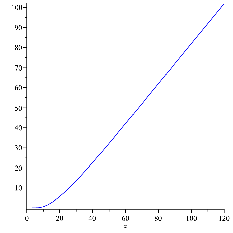
Finally we demonstrate the comparison of restricted and unrestricted payment schemes through a numerical example, in which $\alpha=1$ , $\delta=0.1$ , $c=4$ , $\lambda=2$ , and $u_{0}=3$ . Note that both (4.1) and (4.7) are satisfied and the threshold and barrier levels are determined to be $d=6.291707724$ and $b=7.004651047$ , respectively. The resulting unrestricted and restricted value functions $V(x)$ and $V_{R}(x)$ are shown in Figure 1(a). We also plot the difference $V(x)-V_{R}(x)$ in Figure 1(b). Note that the plot of $V_{R}(x)$ in Figure 1(a) also demonstrates the limit result of $V_{R}(x)$ stated in Lemma 2.1.

Refer to caption — (a) Value functions $V(x)$ and $V_{R}(x)$

4.2 Classical Model with Constant Interest

In this case, we consider $g(x)=\rho x+c$ , where $\rho,\,c$ are positive constants. Note that the first condition (2.11) in Theorem 2.5 is

\alpha\lambda c+(\rho-\lambda-\delta)(\lambda+\delta)>0.

(4.8)

And the second condition (2.12) is satisfied if and only if

\rho<\delta.

(4.9)

We now need to find a solution $\psi_{1}(x)$ to the IDE

(\rho x+c)\psi^{\prime}(x)-(\lambda+\delta)\psi(x)+\lambda\int^{x}_{0}\psi(x-y)\alpha e^{-\alpha y}\,\mathrm{d}y=0,\qquad x>0,

(4.10)

and an increasing and concave solution $\psi_{2}(x)$ to the ODE

(\rho x+c-u_{0})\psi^{\prime\prime}(x)+[\alpha(\rho x+c)-\alpha u_{0}+\rho-(\lambda+\delta)]\psi^{\prime}(x)-\alpha\delta\psi(x)=0,\qquad x>0.

(4.11)

Applying $(\,\mathrm{d}/\,\mathrm{d}x+\alpha)$ to both sides of (4.10) gives

(\rho x+c)\psi^{\prime\prime}(x)+[\alpha(\rho x+c)+\rho-\lambda-\delta]\psi^{\prime}(x)-\alpha\delta\psi(x)=0.

(4.12)

Then a fundamental system of (4.12) is given by

p_{1}(x)=z^{b-1}e^{-z}M(a,b,z),\qquad p_{2}(x)=z^{b-1}e^{-z}U(a,b,z),

where $M$ and $U$ are the Kummer’s functions of the first and second kind respectively, and

z=\frac{\alpha}{\rho}(\rho x+c),\qquad a=1+\frac{\delta}{\rho}>0,\qquad b=1+\frac{\lambda+\delta}{\rho}>0.

Using (Olver et al.,, 2010, p.325-326, (13.3.20),(13.3.27)),

\displaystyle\frac{\,\mathrm{d}}{\,\mathrm{d}z}(e^{-z}M(a,b,z))

\displaystyle=(-1)\frac{b-a}{b}e^{-z}M(a,b+1,z),\quad\frac{\,\mathrm{d}}{\,\mathrm{d}z}(e^{-z}U(a,b,z))

\displaystyle=(-1)e^{-z}U(a,b+1,z),

it is easy to show that

	$\displaystyle cp^{\prime}_{1}(0)-(\lambda+\delta)p_{1}(0)$	$\displaystyle=-\left(\frac{\alpha c}{\rho}\right)^{b}\frac{\lambda\rho}{\rho+\lambda+\delta}e^{-\alpha c/\rho}M\left(a,b+1,\frac{\alpha c}{\rho}\right),$
	$\displaystyle cp^{\prime}_{2}(0)-(\lambda+\delta)p_{2}(0)$	$\displaystyle=-\left(\frac{\alpha c}{\rho}\right)^{b}\rho e^{-\alpha c/\rho}U\left(a,b+1,\frac{\alpha c}{\rho}\right).$

It follows from (4.10) that $c\psi^{\prime}(0)-(\lambda+\delta)\psi(0)=0$ . Hence the unique solution to (4.10) up to a multiplicative constant is given by

\psi_{1}(x)=K_{1}p_{1}(x)-K_{2}p_{2}(x).

where

K_{1}=(\rho+\lambda+\delta)U\left(a,b+1,\frac{\alpha c}{\rho}\right),\qquad K_{2}=\lambda M\left(a,b+1,\frac{\alpha c}{\rho}\right).

By (Olver et al.,, 2010, p.326, (13.3.28)),

\frac{\,\mathrm{d}^{n}}{\,\mathrm{d}z^{n}}(z^{b-1}e^{-z}U(a,b,z))=(-1)^{n}z^{b-n-1}e^{-z}U(a-n,b-n,z),

we see that an increasing and concave solution to (4.11) is given by

\psi_{2}(x)=-p^{\ast}_{2}(x)=-(z^{\ast})^{b-1}e^{-z^{\ast}}U(a,b,z^{\ast}),\qquad\mbox{ where }z^{\ast}=\frac{\alpha}{\rho}(\rho x+c-u_{0}).

4.2.1 Restricted Payment Scheme

We want to determine the unique number $d>0$ for which equation (2.7) holds. Among other equivalent conditions, one sufficient and necessary condition for $d>0$ is

\displaystyle\frac{\alpha}{\rho}(c-u_{0})\frac{U\left(1+\delta/\rho,1+(\lambda+\delta)/\rho,\alpha(c-u_{0})/\rho\right)}{U\left(\delta/\rho,(\lambda+\delta)/\rho,\alpha(c-u_{0})/\rho\right)}<\frac{u_{0}(\lambda+\delta)-c\delta}{(\lambda+\delta)\delta}.

(4.13)

According to Theorem 2.5(i), under the conditions (4.8), (4.9), (4.13), the value function is given by

V_{R}(x)=\begin{cases}\displaystyle\frac{K_{1}\,p_{1}(x)-K_{2}\,p_{2}(x)}{K_{1}C_{1}(d)+K_{2}C_{2}(d)}&\quad\text{ if }0\leq x<d;\\[2.15277pt] \displaystyle\frac{u_{0}}{\delta}-\frac{p^{\ast}_{2}(x)}{C_{3}(d)}&\quad\text{ if }x\geq d,\end{cases}

where $C_{1}(\cdot),C_{2}(\cdot),C_{3}(\cdot)$ are positive functions given by

	$\displaystyle C_{1}(d)$	$\displaystyle=\frac{\lambda+\delta}{\rho}\left(\alpha d+\frac{\alpha c}{\rho}\right)^{(\lambda+\delta)/\rho-1}\exp\left\{-\alpha d+\frac{\alpha c}{\rho}\right\}M\left(\frac{\delta}{\rho},\frac{\lambda+\delta}{\rho},\alpha d+\frac{\alpha c}{\rho}\right);$
	$\displaystyle C_{2}(d)$	$\displaystyle=\left(\alpha d+\frac{\alpha c}{\rho}\right)^{(\lambda+\delta)/\rho-1}\exp\left\{-\alpha d+\frac{\alpha c}{\rho}\right\}U\left(\frac{\delta}{\rho},\frac{\lambda+\delta}{\rho},\alpha d+\frac{\alpha c}{\rho}\right);$
	$\displaystyle C_{3}(d)$	$\displaystyle=\left[\alpha d+\frac{\alpha}{\rho}(c-u_{0})\right]^{(\lambda+\delta)/\rho-1}\!\!\exp\left\{-\alpha d+\frac{\alpha}{\rho}(c-u_{0})\right\}U\left(\frac{\delta}{\rho},\frac{\lambda+\delta}{\rho},\alpha d+\frac{\alpha}{\rho}(c-u_{0})\right).$

If (4.13) is violated, it follows from Theorem 2.5(ii) that the value function is given by

V_{R}(x)=\frac{u_{0}}{\delta}-\frac{p^{\ast}_{2}(x)}{K},\qquad x\geq 0,

where

\displaystyle K=

\displaystyle\Big(\frac{\alpha(c-u_{0})}{\rho}\Big)^{1+(\lambda+\delta)/\rho}e^{-\alpha(c-u_{0})/\rho}\left(\frac{\delta\rho}{\lambda u_{0}}\right)U\left(\frac{\delta}{\rho}+1,\frac{\lambda+\delta}{\rho}+2,\frac{\alpha(c-u_{0})}{\rho}\right).

4.2.2 Unrestricted Payment Scheme

Note that $\psi_{1}(x)$ solves the IDE (4.10). Using (Olver et al.,, 2010, p.325-326, (13.3.21), (13.3.28)), we can determine the unique minimum value of $\psi^{\prime}_{1}(x)$ at $b$ by solving the equation

\begin{array}[]{rl}K_{1}\left(\frac{\lambda+\delta}{\rho}-1\right)&\!\!\!\displaystyle\left(\frac{\lambda+\delta}{\rho}\right)M\left(\frac{\delta}{\rho}-1,\frac{\lambda+\delta}{\rho}-1,\alpha b+\frac{\alpha c}{\rho}\right)\\ &\displaystyle+K_{2}U\left(\frac{\delta}{\rho}-1,\frac{\lambda+\delta}{\rho}-1,\alpha b+\frac{\alpha c}{\rho}\right)=0.\end{array}

According to Theorem 3.7(i), under conditions (4.8) and (4.9), we must have $b>0$ and that the dividend payment policy defined in (3.9) is optimal and the value function is given by

V(x)=\begin{cases}\displaystyle\frac{K_{1}\,p_{1}(x)-K_{2}\,p_{2}(x)}{K_{1}C_{1}(b)+K_{2}C_{2}(b)}&\quad\text{ if }0\leq x<b;\\[2.15277pt] \displaystyle x-b+\frac{K_{1}\,p_{1}(b)-K_{2}\,p_{2}(b)}{K_{1}C_{1}(b)+K_{2}C_{2}(b)},&\quad\text{ if }x\geq b.\end{cases}

In the case when $\alpha\lambda c+(\rho-\lambda-\delta)(\lambda+\delta)\leq 0,$ Theorem 3.7(ii) tells us that the value function of the optimal payment scheme is

V(x)=x+\frac{c}{\lambda+\delta},\qquad x\geq 0.

Last, we make a comparison of the optimal restricted and unrestricted payment schemes developed in this model with a numerical example. The parameters are chosen as follows: $\rho=0.05,\lambda=1,\delta=0.06,\alpha=1,c=2$ , and $u_{0}=1.5.$ Note that all three conditions (4.8), (4.9) and (4.13) are satisfied, which guarantees the existence and uniqueness of the constants $0<d<b$ . In this example, we calculate $d=8.660487436$ and $b=9.870353657.$ The comparison of the value functions of both optimal unrestricted and restricted dividend policies are plotted in Figure 2(a) and their difference shown in Figure 2(b).

4.3 Regressive growth model

We consider a risk model with a regressive growth rate. Assume that the growth rate $g$ of the overall insurance business depends on the insurance surplus and can be adjusted by changing the premium rates according to the following stochastic differential equation. For $b>0$ ,

\,\mathrm{d}g(X_{t})=b[c-g(X_{t})]\,\mathrm{d}X_{t}.

When the growth rate is below a normal rate $c>0$ , the incremental growth is accelerated. When the growth rate is above the normal rate $c$ , the incremental growth is reduced. An application of Ito’s formula shows that

g(X_{t})=ae^{-bX_{t}}+c,\qquad\mbox{ where }a=g(0)-c.

Since a high premium is charged when the surplus is low, we assume that $a>0$ .

We are now interested in finding the optimal dividend payment schemes in the risk model (1.2) with $g(x)=ae^{-bx}+c$ where $a,b>0$ and $c>u_{0}\geq 0$ . In this case, the first condition (2.11) in Theorem 2.5 translates to

\displaystyle\alpha\lambda(a+c)-(ab+\lambda+\delta)(\lambda+\delta)>0.

(4.14)

The second condition (2.12) is true if and only if

\displaystyle ab(b-\alpha)<\alpha\delta.

(4.15)

We look for a non-trivial solution $\psi_{1}$ to the IDE (which is positive and increasing if $\psi_{1}(0)>0$ , and negative and decreasing if $\psi_{1}(0)<0$ by Lemma 2.3)

\displaystyle(ae^{-bx}+c)\psi^{\prime}(x)-(\lambda+\delta)\psi(x)+\lambda\int^{x}_{0}\psi(x-y)\alpha e^{-\alpha y}\,\mathrm{d}y=0,\qquad x>0,

(4.16)

and an increasing and concave solution $\psi_{2}$ to the ODE

\displaystyle(ae^{-bx}+c-u_{0})\psi^{\prime\prime}(x)+[a(\alpha-b)e^{-bx}+\alpha(c-u_{0})-\lambda-\delta]\psi^{\prime}(x)-\alpha\delta\psi(x)=0.

(4.17)

Applying $(\,\mathrm{d}/\,\mathrm{d}x+\alpha)$ to (4.16) and letting $z=(-c/a)e^{bx},y(z)=\psi(x)$ , we arrive at the Gauss’ hypergeometric equation

z(z-1)y^{\prime\prime}(z)+\left[(k_{1}+k_{2}+1)z-\frac{\alpha}{b}\right]y^{\prime}(z)+k_{1}k_{2}y(z)=0,

where

k_{1}=\frac{\alpha c-\lambda-\delta+\sqrt{(\alpha c-\lambda-\delta)^{2}+4\alpha\delta c}}{2bc},\qquad k_{2}=\frac{\alpha c-\lambda-\delta-\sqrt{(\alpha c-\lambda-\delta)^{2}+4\alpha\delta c}}{2bc}.

The equation has regular singularities at $z=0,1,\infty$ and (Olver et al.,, 2010, p.395) give six solutions, among which the following two will be used:

F\left(k_{1},k_{2};\frac{\alpha}{b};z\right),\qquad z^{-k_{1}}F\left(k_{1},k_{1}-\frac{\alpha}{b}+1;k_{1}-k_{2}+1,\frac{1}{z}\right),

where $F(a,b;c;z)$ is the hypergeometric function. Since $k_{1}>\alpha/b>0$ and $\alpha/b>k_{2}$ , one can show that both solutions are well-defined and linearly independent and thus form a fundamental system of solutions to the hypergeometric equation. We obtain the solution to (4.16)

\displaystyle\psi(x)=C_{1}f_{1}(x)-C_{2}f_{2}(x).

where

\displaystyle f_{1}(x)=F\left(k_{1},k_{2};\frac{\alpha}{b};-\frac{c}{a}e^{bx}\right),\qquad f_{2}(x)=e^{-bk_{1}x}F\left(k_{1},k_{1}-\frac{\alpha}{b}+1;k_{1}-k_{2}+1;-\frac{a}{c}e^{-bx}\right),

subject to the initial condition that

\displaystyle(a+c)\psi^{\prime}_{1}(0)-(\lambda+\delta)\psi_{1}(0)=0.

(4.18)

It follows from (Olver et al.,, 2010, p.387, (15.5.1))

\frac{\,\mathrm{d}}{\,\mathrm{d}z}F(a,b;c;z)=\frac{ab}{c}F(a+1,b+1;c+1;z)

that the derivative of $f_{1}$ is given by

$\displaystyle f^{\prime}_{1}(x)$	$\displaystyle=$	$\displaystyle\frac{\delta}{a}e^{bx}F\left(k_{1}+1,k_{2}+1;\frac{\alpha}{b}+1;-\frac{c}{a}e^{bx}\right);$
$\displaystyle f^{\prime\prime}_{1}(x)$	$\displaystyle=$	$\displaystyle\frac{b\delta}{a}e^{bx}F\left(k_{1}+1,k_{2}+1;\frac{\alpha}{b}+1;-\frac{c}{a}e^{bx}\right)$
		$\displaystyle-\frac{\delta(\alpha bc+b^{2}c-\alpha\delta-b\lambda-b\delta)}{a^{2}(\alpha+b)}e^{2bx}F\left(k_{1}+2,k_{2}+2;\frac{\alpha}{b}+2;-\frac{c}{a}e^{bx}\right).$

Using (Olver et al.,, 2010, p.387, (15.5.3)) with $n=1$ ,

\frac{\,\mathrm{d}}{\,\mathrm{d}z}\big((z^{a}F(a,b;c;z)\big)=az^{a-1}F(a+1,b;c;z),

we find the first two derivatives of $f_{2}$

	$\displaystyle f^{\prime}_{2}(x)=$	$\displaystyle-bk_{1}e^{-bk_{1}x}F\left(k_{1}+1,k_{1}-\frac{\alpha}{b}+1;k_{1}-k_{2}+1;-\frac{a}{c}e^{-bx}\right),$
	$\displaystyle f^{\prime\prime}_{2}(x)=$	$\displaystyle(bk_{1})^{2}e^{-bk_{1}x}F\left(k_{1}+1,k_{1}-\frac{\alpha}{b}+1;k_{1}-k_{2}+1;-\frac{a}{c}e^{-bx}\right)$
		$\displaystyle-\frac{ab^{2}k_{1}(k_{1}+1)(k_{1}-\alpha/b+1)}{c(k_{1}-k_{2}+1)}e^{-b(k_{1}+1)x}F\left(k_{1}+2,k_{1}-\frac{\alpha}{b}+2;k_{1}-k_{2}+2;-\frac{a}{c}e^{-bx}\right).$

Using (Olver et al.,, 2010, p.388, (15.5.21))

c(1-z)\frac{\,\mathrm{d}}{\,\mathrm{d}z}F(a,b;c;z)=(c-a)(c-b)F(a,b;c+1;z)+c(a+b-c)F(a,b,c;z),

we obtain

\displaystyle(a+c)f^{\prime}_{1}(0)-(\lambda+\delta)f_{1}(0)=-\lambda F\left(k_{1},k_{2};\frac{\alpha}{b}+1;-\frac{c}{a}\right).

(4.19)

Using (Olver et al.,, 2010, p.388, (15.5.13))

\displaystyle(c-a-b)F(a,b;c;z)+a(1-z)F(a+1,b;c;z)-(c-b)F(a,b-1;c;z)=0,

we get

\displaystyle(a+c)f^{\prime}_{2}(0)-(\lambda+\delta)f_{2}(0)=(bk_{2}-\alpha)cF\left(k_{1},k_{1}-\frac{\alpha}{b};k_{1}-k_{2}+1;-\frac{a}{c}\right).

(4.20)

Substituting (4.19), (4.20) into (4.18) determines the unique solution to (4.16) up to a multiplicative constant

\psi_{1}(x)=C_{1}f_{1}(x)-C_{2}f_{2}(x),

where $C_{1}$ and $C_{2}$ are positive constants given by

\displaystyle C_{1}=\left(\alpha-bk_{2}\right)cF\left(k_{1},k_{1}-\frac{\alpha}{b};k_{1}-k_{2}+1;-\frac{a}{c}\right),\qquad C_{2}=\lambda F\left(k_{1},k_{2};\frac{\alpha}{b}+1;-\frac{c}{a}\right).

We claim that a negative, increasing and concave solution to (4.17) is given by

\psi_{2}(x)=-f^{\ast}_{2}(x):=-e^{-bk^{\ast}_{1}x}F\left(k^{\ast}_{1},k^{\ast}_{1}-\frac{\alpha}{b}+1;k^{\ast}_{1}-k^{\ast}_{2}+1;-\frac{a}{c-u_{0}}e^{-bx}\right),

where

	$\displaystyle k^{\ast}_{1}=\frac{\alpha(c-u_{0})-\lambda-\delta+\sqrt{(\alpha(c-u_{0})-\lambda-\delta)^{2}+4\alpha\delta(c-u_{0})}}{2b(c-u_{0})},$
	$\displaystyle k^{\ast}_{2}=\frac{\alpha(c-u_{0})-\lambda-\delta-\sqrt{(\alpha(c-u_{0})-\lambda-\delta)^{2}+4\alpha\delta(c-u_{0})}}{2b(c-u_{0})}.$

It follows from the definition of the hypergeometric function that $f^{\ast}_{2}(x)>0$ and $(f^{\ast}_{2})^{\prime}(x)<0$ for large $x$ . Suppose there exists $x_{0}:=\inf\{x\geq 0:(f^{\ast}_{2})^{\prime}(x)=0,f^{\ast}_{2}(x)\geq 0\}.$ Recall that $f^{\ast}_{2}$ is a solution to the ODE (4.17). Since $ae^{-bx_{0}}+c-u_{0}>0$ and $-\alpha\delta<0,$ we must have $(f^{\ast}_{2})^{\prime\prime}(x_{0})\geq 0$ which leads to a contradiction. Thus $(f^{\ast}_{2})^{\prime}(x)<0,f^{\ast}_{2}(x)>0$ for all $x\geq 0$ . To show the sign of $(f^{\ast}_{2})^{\prime\prime}$ , we differentiate (4.17) with respect to $x$ and observe that $f^{\ast}_{2}$ satisfies

A(x)f^{\prime\prime\prime}(x)+B(x)f^{\prime\prime}(x)+C(x)f^{\prime}(x)=0,

where $A(x)=ae^{-bx}+c-u_{0}>0,C(x)=ab(b-\alpha)e^{-bx}-\alpha\delta<0$ for $x\geq 0$ due to (4.15). We can conclude in the same way as before that $(f^{\ast}_{2})^{\prime\prime}(x)>0$ for all $x\geq 0$ . Therefore, $\psi_{2}$ is indeed negative, increasing and concave.

4.3.1 Restricted Payment Scheme

Consider the restricted payment scheme under which the dividend rate is capped at $0<u_{0}<c$ . Then we can determine the optimal dividend strategy according to Theorem 2.5. The condition (2.13) reduces to

\displaystyle\frac{F(k^{\ast}_{1},k^{\ast}_{1}-\alpha/b+1;k^{\ast}_{1}-k^{\ast}_{2}+1;-a/(c-u_{0}))}{bk^{\ast}_{1}F(k^{\ast}_{1}+1,k^{\ast}_{1}-\alpha/b+1;k^{\ast}_{1}-k^{\ast}_{2}+1;-a/(c-u_{0}))}<\frac{u_{0}(\lambda+\delta)-(a+c)\delta}{(\lambda+\delta)\delta}.

(4.21)

Therefore, under conditions (4.14), (4.15), (4.21), the optimal value function is given by

\displaystyle V_{R}(x)=\left\{\begin{array}[]{ll}\displaystyle\frac{C_{1}f_{1}(x)-C_{2}f_{2}(x)}{C_{1}e_{1}(d)+C_{2}e_{2}(d)},&\mbox{ if }0\leq x<d;\\ \displaystyle\frac{u_{0}}{\delta}-\frac{f^{\ast}_{2}}{e_{3}(d)},&\mbox{ if }x\geq d,\end{array}\right.

where $e_{1},e_{2},e_{3}$ are positive functions given by

$\displaystyle e_{1}(d)$	$\displaystyle=$	$\displaystyle\frac{\delta}{a}e^{bd}F\left(k_{1}+1,k_{2}+1;\frac{\alpha}{b}+1;-\frac{c}{a}e^{bd}\right);$
$\displaystyle e_{2}(d)$	$\displaystyle=$	$\displaystyle bk_{1}e^{-bk_{1}d}F\left(k_{1}+1,k_{1}-\frac{\alpha}{b}+1;k_{1}-k_{2}+1;-\frac{a}{c}e^{-bd}\right);$
$\displaystyle e_{3}(d)$	$\displaystyle=$	$\displaystyle bk^{\ast}_{1}e^{-bk_{1}d}F\left(k^{\ast}_{1}+1,k^{\ast}_{1}-\frac{\alpha}{b}+1;k^{\ast}_{1}-k^{\ast}_{2}+1;-\frac{a}{c-u_{0}}e^{-bd}\right).$

If (4.21) is not true, then the value function is given by

V_{R}(x)=\frac{u_{0}}{d}-\frac{f^{\ast}_{2}(x)}{K},\qquad x\geq 0,

where

\displaystyle K=\frac{\delta(bk^{\ast}_{2}-\alpha)(c-u_{0})}{\lambda u_{0}}F\left(k^{\ast}_{1},k^{\ast}_{1}-\frac{\alpha}{b};k^{\ast}_{1}-k^{\ast}_{2}+1;-\frac{a}{c-u_{0}}\right).

4.3.2 Unrestricted Payment Scheme

In this case there is no restriction on the dividend payment rate. According to Theorem 3.6, we first determine the minimum of $\psi^{\prime}_{1}$ at $x^{\ast}$ by

	$\displaystyle\lx@add@cssclass{ltx_eqn_lefteqn}$\displaystyle C_{1}\frac{b\delta}{a}e^{bx^{\ast}}F\left(k_{1}+1,k_{2}+1;\frac{\alpha}{b}+1;-\frac{c}{a}e^{bx}\right)$\mbox{}$
		$\displaystyle-C_{1}\frac{\delta(\alpha bc+b^{2}c-\alpha\delta-b\lambda-b\delta)}{a^{2}(\alpha+b)}F\left(k_{1}+2,k_{2}+2;\frac{\alpha}{b}+2;-\frac{c}{a}e^{bx^{\ast}}\right)$
		$\displaystyle-C_{2}(bk_{1})^{2}e^{-bk_{1}x^{\ast}}F\left(k_{1}+1,k_{1}-\frac{\alpha}{b}+1;k_{1}-k_{2}+1;-\frac{a}{c}e^{-bx^{\ast}}\right)$
		$\displaystyle+C_{2}\frac{ab^{2}k_{1}(k_{1}+1)(k_{1}-\alpha/b+1)}{c(k_{1}-k_{2}+1)}e^{-b(k_{1}+1)x^{\ast}}F\left(k_{1}+2,k_{1}-\frac{\alpha}{b}+2;k_{1}-k_{2}+2;-\frac{a}{c}e^{-bx^{\ast}}\right)=0.$

The existence and uniqueness of such a value $x^{\ast}$ is guaranteed by conditions (4.14) and (4.15) according to Theorem 3.7(i). Thus the optimal value function is given by

\displaystyle V(x)=\left\{\begin{array}[]{ll}\displaystyle\frac{C_{1}f_{1}(x)-C_{2}f_{2}(x)}{C_{1}e_{1}(x^{\ast})+C_{2}e_{2}(x^{\ast})},&\mbox{ if }0\leq x<x^{\ast};\\ \displaystyle x-x^{\ast}-\frac{C_{1}f_{1}(x^{\ast})-C_{2}f_{2}(x^{\ast})}{C_{1}e_{1}(x^{\ast})+C_{2}e_{2}(x^{\ast})},&\mbox{ if }x\geq x^{\ast},\end{array}\right.

In the case where $\alpha\lambda(a+c)-(ab+\lambda+\delta)(\lambda+\delta)\geq 0$ , Theorem 3.7(ii) tells us that the barrier level is $0$ and the optimal value function is given by

V(x)=x+\frac{a+c}{\lambda+\delta},\qquad x\geq 0.

Here we give a numerical example of the optimal dividend payment schemes with regressive premium rates. The parameters are chosen as follows: $a=2,b=0.15,c=2,\lambda=1,\alpha=1,$ and $\delta=0.06$ . All conditions (4.14), (4.15), (4.21) are satisfied. The values of $d=0.2143382330$ and $x^{\ast}=5.324276475$ are determined numerically by a root search method. The value functions $V(x),V_{R}(x)$ , and their difference are plotted in Figure 3.

5 Conclusions and Remarks

This work is devoted to the optimal dividend payment problems for the PDCP risk model. Both restricted and unrestricted dividend schemes are investigated and compared. We provide easily verifiable conditions under which the threshold and barrier strategies are optimal restricted and unrestricted dividend payment policies, respectively. Our analysis is primarily based on the qualitative properties of solutions to certain IDE and ODE associated with a general PDCP risk model. Three examples are demonstrated to illustrate the main results.

A number of questions deserve further investigations. One can consider more general models in which the parameters and hence the dynamics of the surplus level depend on a stochastic process such as a continuous-time Markov chain. In such a case, we need to deal with regime-switching jump diffusions (see Yin and Zhu, (2010)) and the resulting HJB equation will be a coupled system of nonlinear integro-differential equations. It is conceivable that it will be more challenging to obtain the corresponding value function and optimal dividend policy in closed forms. Some initial work in this vein can be found in Zhu, (2011) using the viscosity solution approach. Another problem of interest is to consider transaction costs, reinsurance, and/or investments. Similar work in the setting of controlled diffusions can be found in Bai and Paulsen, (2010), Choulli et al., (2003), etc.

Appendix A Appendix

We prove two technical lemmas on the properties of the solution to the ODE (A.1), which will enable us to identify optimal dividend strategies in a general PDCP model. Consider

f(x)u^{\prime\prime}(x)+h(x)u^{\prime}(x)-ku(x)=0,\qquad x\geq 0

(A.1)

where $f,h:[0,\infty)\rightarrow{\mathbb{R}}$ are continuously differentiable and $f(x)>0$ for all $x\geq 0$ and $k>0$ .

Lemma A.1.

Let $u$ be a solution of (A.1) such that

(i)

$u(0)>0,u^{\prime}(0)>0,u^{\prime\prime}(0)<0;$
(ii)

There exists $m<k$ such that $h^{\prime}(x)\leq m$ for all $x>0$ .

Then there is a unique $b>0$ such that $u(x)$ is concave for $0\leq x<b$ and convex for $x>b$ .

Proof.

First, we show that $u(x)>0$ and $u^{\prime}(x)>0$ for all $x\geq 0$ . Since $u(0)>0$ and $u^{\prime}(0)>0,$ $u(x)>0$ and $u^{\prime}(x)>0$ for small $x>0.$ Suppose there exists $x_{0}>0$ such that $u^{\prime}(x_{0})=0$ and $u^{\prime}(x)>0$ for all $x\in(0,x_{0})$ , then $u^{\prime\prime}(x_{0})\leq 0$ . It follows from (A.1) that $u^{\prime\prime}(x_{0})=ku(x_{0})/f(x_{0})>0$ which leads to a contradiction. Hence the claim is proved.

Then, we prove by contradiction that there exists $b>0$ such that $u^{\prime\prime}(b)=0$ . Suppose that $u^{\prime\prime}(x)$ has no zero. Since $u^{\prime\prime}(0)<0$ , $u^{\prime\prime}(x)<0$ for all $x\geq 0$ . Let $A=\max\{m/k,1/2\}<1$ . Since $h^{\prime}(x)\leq m$ for all $x>0$ , there must exist $B>0$ such that $h(x)/k\leq(m/k)x+h(0)/k\leq Ax+B.$ It follows from (A.1) that

(Ax+B)u^{\prime}(x)\geq\frac{h(x)}{k}u^{\prime}(x)>u(x)\qquad\mbox{ for all }x\geq 0.

(A.2)

Dividing (A.2) by $(Ax+B)u(x)>0$ and integrating from $0$ to $x$ , we obtain $u(x)\geq u(0)\left(\frac{Ax+B}{B}\right)^{1/A},$ which implies

u^{\prime}(x)\geq(Ax+B)^{-1}u(x)\geq u(0)B^{-1/A}(Ax+B)^{1/A-1}\rightarrow\infty,\qquad x\rightarrow\infty.

This is impossible because $u^{\prime}(x)$ is a decreasing function. The contradiction shows that $u^{\prime\prime}(x)$ has a positive zero.

Last, we show that $u^{\prime\prime}(x)$ has a unique zero. Suppose that $u^{\prime\prime}(x)$ does have a second zero $x_{1}>b$ such that $u^{\prime\prime}(x)>0$ for all $x\in(b,x_{1})$ and $u^{\prime\prime}(x_{1})=0$ . Hence it must be true that $u^{\prime\prime\prime}(x_{1})\leq 0$ . Differentiating (A.1), we obtain

f(x)u^{\prime\prime\prime}(x)+(f^{\prime}(x)+h(x))u^{\prime\prime}(x)+(h^{\prime}(x)-k)u^{\prime}(x)=0.

(A.3)

Therefore, we must also have $u^{\prime\prime\prime}(x_{1})=(k-h^{\prime}(x_{1}))u^{\prime}(x_{1})/f(x_{1})>0$ since $u^{\prime}(x)>0$ for all $x\geq 0$ . This contradiction implies the uniqueness of the zero of $u^{\prime\prime}(x)$ . $\Box$

Lemma A.2.

Assume that there exists a constant $m<k$ such that $h^{\prime}(x)\leq m$ for all $x\geq 0$ . Then equation (A.1) admits a solution $u$ such that

u(x)<0,\,u^{\prime}(x)>0,\,u^{\prime\prime}(x)<0\,\mbox{ for all }x\geq 0.

Proof.

Let $v(x)=u^{\prime}(x)$ in equation (A.3). We obtain

f(x)v^{\prime\prime}(x)+(f^{\prime}(x)+h(x))v^{\prime}(x)+(h^{\prime}(x)-k)v(x)=0.

(A.4)

Since $h^{\prime}(x)\leq m<k$ for all $x\geq 0$ , it follows from Corollary 1.2 in Chapter XIV of Hartman, (2002) that (A.4) has at least one solution $v(x)$ satisfying $v(x)>0,v^{\prime}(x)\leq 0$ for all $x\geq 0$ . If there exists $x_{2}\geq 0$ such that $v^{\prime}(x_{2})=0$ , then we must have $v^{\prime\prime}(x_{2})\leq 0$ . Note that it follows from (A.4) that $v^{\prime\prime}(x_{2})=(k-h^{\prime}(x_{2}))v(x_{2})/f(x_{2})>0,$ which causes a contradiction. Therefore, we must have $v(x)>0,v^{\prime}(x)<0$ for all $x\geq 0$ . There is a function $u(x)$ such that $u^{\prime}(x)=v(x)$ and $u(x)$ satisfies (A.1). Thus, for such a solution $u(x)$ , we must have $u^{\prime}(x)>0,u^{\prime\prime}(x)<0$ for all $x\geq 0$ .

Next, we show that $u(x)<0$ for all $x\geq 0$ . Suppose there exists $x_{3}\geq 0$ such that $u(x_{3})\geq 0$ . Then we must have $u(x_{4})>0,u^{\prime}(x_{4})>0,u^{\prime\prime}(x_{4})<0$ for some $x_{4}>x_{3}$ . Let $w(x)=u(x-x_{4}),f_{w}(x)=f(x-x_{4}),h_{w}(x)=h(x-x_{4}).$ Then $w(x)$ must satisfy the ODE

f_{w}(x)w^{\prime\prime}(x)+h_{w}(x)w^{\prime}(x)-kw(x)=0,\qquad x\geq 0,

and all conditions in Lemma A.1 are satisfied. Hence there must exist $x_{5}>0$ such that $u^{\prime\prime}(x_{4}+x_{5})=w^{\prime\prime}(x_{5})=0$ which contradicts the fact that $u^{\prime\prime}(x)<0$ for all $x\geq 0$ . Therefore, it must be true that $u(x)<0$ for all $x\geq 0$ . $\Box$

Proof of Lemma 2.1.

That the function $V_{R}(x)$ is bounded by $u_{0}/\delta$ is obvious. Also, monotonicity can be established by considering two surplus processes with different initial surplus levels and the same dividend payment schemes. The rest of the proof is divided into two steps.

Step 1. (Lipschitz Continuity) Let $h$ be a small positive value and $\tilde{D}\in\Pi_{R}$ be an arbitrary strategy. Define another strategy $D\in\Pi_{R}$ so that $D(t)=\tilde{D}(t-h)I_{\left\{T_{1}\wedge t>h\right\}}.$ Denote by $X(t)$ the surplus process with initial surplus $x>0$ under the dividend payment strategy $D$ . It is clear that if $T_{1}>h$ , then the surplus at time $h$ is $X(h)=\phi_{x}(h)$ . Therefore it follows that $V_{R}(x)\geq J(x,D)\geq e^{-(\lambda+\delta)h}J(\phi_{x}(h),\tilde{D}),$ which implies by taking the supremum over all possible strategies $\tilde{D}\in\Pi_{R}$ that

\displaystyle V_{R}(x)\geq e^{-(\lambda+\delta)h}V_{R}(\phi_{x}(h))\geq e^{-(\lambda+\delta)h}V_{R}(x),

(A.5)

with the last inequality from the fact that $V_{R}(x)$ is an increasing function and $g(x)\geq 0.$ Thus $V_{R}(x)$ is right continuous by the continuity of $\phi_{x}(h)$ and the squeeze theorem. Replacing $x$ with $\phi_{x}(-h)$ in (A.5), we obtain

\displaystyle V_{R}(\phi_{x}(-h))\geq e^{-(\lambda+\delta)h}V_{R}(x)\geq e^{-(\lambda+\delta)h}V_{R}(\phi_{x}(-h)).

Hence left continuity follows. Now it follows from (A.5) that

0\leq V_{R}(\phi_{x}(h))-V_{R}(x)\leq(1-e^{-(\lambda+\delta)h})V_{R}(\phi_{x}(h))\leq(1-e^{-(\lambda+\delta)h})u_{0}/\delta.

Therefore, $V_{R}(x)$ is indeed Lipschitz continuous.

Step 2. (Limit at $\infty$ ) Let $D(t):=u_{0}t$ for all $t\geq 0$ . Denote the surplus process by $X(t)$ under the strategy $D$ and initial surplus $x>0$ and by $\tau$ the corresponding time of ruin. Then as $x\to\infty$ , $\tau$ converges to infinity a.s. Therefore

V_{R}(x)\geq J(x,D)={\mathrm{E}}\int_{0}^{\tau}e^{-\delta t}u_{0}\,\mathrm{d}t=\frac{u_{0}}{\delta}(1-{\mathrm{E}}[e^{-\delta\tau}])\to\frac{u_{0}}{\delta},

this, together with the boundedness of $V_{R}(x)$ , leads to the desired conclusion. $\Box$

Proof of Theorem 2.2.

The proof is motivated by (Schmidli,, 2008, Theorem 2.32). It utilizes Lemma 2.1 and the dynamic programming principle:

\displaystyle V_{R}(x)=\sup_{u(\cdot)\in\Pi_{R}}\mathrm{E}_{x}\left[\int_{0}^{\tau\wedge\theta}e^{-\delta s}u(s)\,\mathrm{d}s+e^{-\delta(\theta\wedge\tau)}V_{R}(X(\theta\wedge\tau))\right],\ \ x\geq 0,

(A.6)

where $\theta$ is an $\mathcal{F}_{t}$ -stopping time.

Step 1. Let $h>0$ and $u\in[0,u_{0}]$ . Let $\{D(t):=ut,t\geq 0\}\in\Pi_{R}.$ Denote

\phi(t,x)=x+\int_{0}^{t}(g(\phi(s,x))-u)\,\mathrm{d}s,\ t\geq 0.

The arrival time $T_{1}$ of the first claim is exponentially distributed with parameter $\lambda$ . Hence we can use the law of total probability and take $\theta=T_{1}\wedge h$ in (A.6) to obtain

	$\displaystyle V_{R}(x)\geq$	$\displaystyle e^{-\lambda h}\bigg[\int^{h}_{0}e^{-\delta t}u\,\mathrm{d}t+e^{-\delta h}V_{R}(\phi(h,x))\bigg]$		(A.7)
		$\displaystyle+\int^{h}_{0}\lambda e^{-\lambda t}\bigg[\int^{t}_{0}e^{-\delta s}u\,\mathrm{d}s+e^{-\delta t}\int^{\phi(t,x)}_{0}V_{R}(\phi(t,x)-y)\,\mathrm{d}Q(y)\bigg]\,\mathrm{d}t.$		(A.7)

Rearranging the terms and dividing by $h$ yields

		$\displaystyle\frac{V_{R}(\phi(h,x))-V_{R}(x)}{h}-\frac{1-e^{-(\lambda+\delta)h}}{h}V_{R}(\phi(h,x))+\frac{e^{-\lambda h}}{h}\int^{h}_{0}e^{-\delta t}u\,\mathrm{d}t$		(A.8)
		$\displaystyle+\frac{1}{h}\int^{h}_{0}\lambda e^{-\lambda t}\bigg[\int^{t}_{0}e^{-\delta s}u\,\mathrm{d}s+e^{-\delta t}\int^{{\phi}(t,x)}_{0}V_{R}(\phi(t,x)-y)\,\mathrm{d}Q(y)\bigg]\,\mathrm{d}t\leq 0.$		(A.8)

Let

\displaystyle D^{+}{V_{R}}(x)=\limsup_{\Delta\rightarrow 0+}\frac{V_{R}(x+\Delta)-V_{R}(x)}{\Delta},\,\,\,D^{-}V_{R}(x)=\liminf_{\Delta\rightarrow 0+}\frac{V_{R}(x+\Delta)-V_{R}(x)}{\Delta}.

Note that $D^{+}{V_{R}}(x)$ and $D^{-}{V_{R}}(x)$ are finite by the Lipschitz continuity of $V_{R}$ . Recall the facts that $0\leq u\leq u_{0}<g(x)$ , $g$ is continuous, $\phi(\cdot,x)$ is strictly increasing and $\phi(t,x)\to x$ as $t\to 0$ . Hence we can choose a sequence $\left\{h_{n},n\geq 1\right\}$ satisfying $h_{n}\to 0$ as $n\to\infty$ and

\lim_{n\to\infty}\frac{V_{R}(\phi(h_{n},x))-V_{R}(x)}{\phi(h_{n},x)-x}=D^{+}V_{R}(x).

By the definition of $\phi(h_{n},x)$ , we have $\phi(h_{n},x)\to x$ as $n\to\infty$ . Also, we have from the continuity of $g$ that as $n\to\infty$

\frac{\phi(h_{n},x)-x}{h_{n}}=\frac{1}{h_{n}}\int_{0}^{h_{n}}\left[g(X(t))-u\right]\,\mathrm{d}t\to g(x)-u.

Hence it follows that

\displaystyle\lim_{n\to\infty}\frac{V_{R}(\phi(h_{n},x))-V_{R}(x)}{h_{n}}

\displaystyle=\lim_{n\to\infty}\frac{V_{R}(\phi(h_{n},x))-V_{R}(x)}{\phi(h_{n},x)-x}\cdot\frac{\phi(h_{n},x)-x}{h_{n}}=D^{+}V_{R}(x)(g(x)-u).

(A.9)

Now taking $h=h_{n}$ in (A.8) and letting $n\to\infty$ , in view of (A.9), detailed calculations reveal that

[g(x)-u]D^{+}V_{R}(x)-(\lambda+\delta)V_{R}(x)+\lambda\int_{0}^{x}V_{R}(x-y)\,\mathrm{d}Q(y)+u\leq 0,\ \ \forall u\in[0,u_{0}].

(A.10)

Step 2. On the other hand, by the definition of $V_{R}$ in (2.2), there exists a strategy $\bar{D}:=\{\int^{t}_{0}\bar{u}(s)\,\mathrm{d}s,t\geq 0\}\in\Pi_{R}$ such that $J(x,\bar{D})\geq V_{R}(x)-h^{2}$ . Denote

\bar{\phi}(t,x)=x+\int^{t}_{0}(g(X(s))-\bar{u}(s))\,\mathrm{d}s.

Then as argued before, we must have

	$\displaystyle V_{R}(x)$	$\displaystyle\leq J(x,\bar{D})+h^{2}$
		$\displaystyle\leq h^{2}+e^{-\lambda h}\left[\int_{0}^{h}e^{-\delta s}\bar{u}(s)\,\mathrm{d}s+e^{-\delta h}V_{R}(\bar{\phi}(h,x))\right]$
		$\displaystyle+\int^{h}_{0}\lambda e^{-\lambda t}\bigg[\int^{t}_{0}e^{-\delta s}\bar{u}(s)\,\mathrm{d}s+e^{-\delta t}\int^{\bar{\phi}(t,x)}_{0}V_{R}(\bar{\phi}(t,x)-y)\,\mathrm{d}Q(y)\bigg]\,\mathrm{d}t.$

We find by rearranging the terms and dividing by $h$ that

\begin{array}[]{ll}&\!\!\!\displaystyle h+\frac{V_{R}(\bar{\phi}(h,x))-V_{R}(x)}{h}-\frac{1-e^{-(\lambda+\delta)h}}{h}V_{R}(\bar{\phi}(h,x))+\frac{e^{-\lambda h}}{h}\int^{h}_{0}e^{-\delta t}\bar{u}(t)\,\mathrm{d}t\\ &\displaystyle+\frac{1}{h}\int^{h}_{0}\lambda e^{-\lambda t}\bigg[\int^{t}_{0}e^{-\delta s}\bar{u}(s)\,\mathrm{d}s+e^{-\delta t}\int^{\bar{\phi}(t,x)}_{0}V_{R}(\bar{\phi}(t,x)-y)\,\mathrm{d}Q(y)\bigg]\,\mathrm{d}t\geq 0.\end{array}

(A.11)

Denote $\bar{u}:=\liminf_{s\to 0+}\bar{u}(s)\in[0,u_{0}].$ Then it follows that

\limsup_{h\to 0+}\frac{\bar{\phi}(h,x)-x}{h}=\limsup_{h\to 0+}\frac{1}{h}\int_{0}^{h}[g(X(s))-\bar{u}(s)]\,\mathrm{d}s\leq g(x)-\bar{u}.

As in Step 1, we can choose a sequence $h_{m}\rightarrow 0+$ such that

\displaystyle\lim_{m\rightarrow\infty}\frac{V_{R}(\bar{\phi}(h_{m},x))-V_{R}(x)}{\bar{\phi}(h_{m},x)-x}=D^{-}V_{R}(x).

Note that $D^{-}V_{R}(x)\geq 0$ by the monotonicity of $V_{R}$ . Then it follows that

\begin{array}[]{ll}\displaystyle\limsup_{m\to\infty}\frac{V_{R}(\bar{\phi}(h_{m},x))-V_{R}(x)}{h_{m}}&\!\!\!\displaystyle=\limsup_{m\to\infty}\frac{V_{R}(\bar{\phi}(h_{m},x))-V_{R}(x)}{\bar{\phi}(h_{m},x)-x}\cdot\frac{\bar{\phi}(h_{m},x)-x}{h_{m}}\\ &\!\!\!\displaystyle\leq D^{-}V_{R}(x)[g(x)-\bar{u}].\end{array}

Now by taking $h=h_{m}$ and letting $m\to\infty$ in (A.11), we obtain

[g(x)-\bar{u}]D^{-}V_{R}(x)-(\lambda+\delta)V_{R}(x)+\lambda\int_{0}^{x}V_{R}(x-y)\,\mathrm{d}Q(y)+\bar{u}\geq 0.

(A.12)

Step 3. Note that $g(x)-\bar{u}\geq g(x)-u_{0}>0$ . Hence, by taking $u=\bar{u}$ in (A.10) and comparing the resulting equation with (A.12), we have $D^{+}V_{R}(x)\leq D^{-}V_{R}(x).$ But $D^{+}V_{R}(x)\geq D^{-}V_{R}(x)$ by definition. Thus it follows that $D^{+}V_{R}(x)=D^{-}V_{R}(x)$ or $V_{R}(x)$ is differentiable from the right. Moreover, a combination of (A.10) and (A.12) yields that $V_{R}^{\prime}(x+)$ , the right derivative of $V_{R}$ , satisfies the HJB equation

\sup_{0\leq u\leq u_{0}}\bigg\{[g(x)-u]V_{R}^{\prime}(x+)-(\lambda+\delta)V_{R}(x)+\lambda\int^{x}_{0}V_{R}(x-y)\,\mathrm{d}Q(y)+u\bigg\}=0.

(A.13)

Similarly, we obtain that the left derivative $V_{R}^{\prime}(x-)$ exists and fulfills the HJB equation

\sup_{0\leq u\leq u_{0}}\left\{[g(x)-u]V_{R}^{\prime}(x-)-(\lambda+\delta)V_{R}(x)+\lambda\int^{x}_{0}V_{R}(x-y)\,\mathrm{d}Q(y)+u\right\}=0.

(A.14)

Step 4. With (A.13) in hands, we claim that

V_{R}^{\prime}(x+)\gtreqqless 1\Leftrightarrow(\lambda+\delta)V_{R}(x)-\lambda\int^{x}_{0}V_{R}(x-y)\,\mathrm{d}Q(y)\gtreqqless g(x).

(A.15)

In fact, if $V_{R}^{\prime}(x+)>1$ , then

\begin{array}[]{rl}0&\!\!\!\displaystyle=\sup_{0\leq u\leq u_{0}}\left\{[g(x)-u]V_{R}^{\prime}(x+)-(\lambda+\delta)V_{R}(x)+\lambda\int^{x}_{0}V_{R}(x-y)\,\mathrm{d}Q(y)+u\right\}\\ &\!\!\!\displaystyle=g(x)V_{R}^{\prime}(x+)-(\lambda+\delta)V_{R}(x)+\lambda\int^{x}_{0}V_{R}(x-y)\,\mathrm{d}Q(y).\end{array}

Hence we have $(\lambda+\delta)V_{R}(x)-\lambda\int^{x}_{0}V_{R}(x-y)\,\mathrm{d}Q(y)=g(x)V_{R}^{\prime}(x+)>g(x).$ Conversely, if $(\lambda+\delta)V_{R}(x)-\lambda\int^{x}_{0}V_{R}(x-y)\,\mathrm{d}Q(y)>g(x)$ , then we have

\begin{array}[]{rl}0&\!\!\!\displaystyle=\sup_{0\leq u\leq u_{0}}\left\{[g(x)-u]V_{R}^{\prime}(x+)-(\lambda+\delta)V_{R}(x)+\lambda\int^{x}_{0}V_{R}(x-y)\,\mathrm{d}Q(y)+u\right\}\\ &\!\!\!\displaystyle<\sup_{0\leq u\leq u_{0}}\left\{(g(x)-u)(V_{R}^{\prime}(x+)-1)\right\}.\end{array}

But $g(x)-u\geq g(x)-u_{0}>0$ . Thus we must have $V_{R}^{\prime}(x+)>1$ . Hence the first case in (A.15) follows. Similar arguments establish the other two cases in (A.15).

Similarly, (A.14) leads to

V_{R}^{\prime}(x-)\gtreqqless 1\Leftrightarrow(\lambda+\delta)V_{R}(x)-\lambda\int^{x}_{0}V_{R}(x-y)\,\mathrm{d}Q(y)\gtreqqless g(x).

(A.16)

Hence, (A.15) and (A.16) imply that $V_{R}^{\prime}(x+)$ and $V_{R}^{\prime}(x-)$ are both less than $1$ , both greater than $1$ , or both equal to $1$ . This, together with the HJB equations (A.13) and (A.14), implies that $V_{R}^{\prime}(x+)=V_{R}^{\prime}(x-)$ and so $V_{R}^{\prime}(x)$ exists. Moreover, the continuities of $V_{R}$ and $g$ implies that $V_{R}^{\prime}(x)$ is continuous. That is, $V_{R}(x)$ is continuously differentiable and satisfies the HJB equation (2.3).

Step 5. Finally, the optimality of the strategy (2.4) is obvious since (2.3) is linear in $u$ . $\Box$

References

Albrecher and Hartinger, (2007) Albrecher, H. and Hartinger, J. (2007). A risk model with multilayer dividend strategy. N. Am. Actuar. J., 11(2):43–64.
Albrecher and Thonhauser, (2008) Albrecher, H. and Thonhauser, S. (2008). Optimal dividend strategies for a risk process under force of interest. Insurance Math. Econom., 43(1):134–149.
Asmussen et al., (2000) Asmussen, S., Højgaard, B., and Taksar, M. (2000). Optimal risk control and dividend distribution policies. Example of excess-of loss reinsurance for an insurance corporation. Finance Stoch., 4(3):299–324.
Asmussen and Taksar, (1997) Asmussen, S. and Taksar, M. (1997). Controlled diffusion models for optimal dividend pay-out. Insurance Math. Econom., 20(1):1–15.
Bai and Paulsen, (2010) Bai, L. and Paulsen, J. (2010). Optimal dividend policies with transaction costs for a class of diffusion processes. SIAM J. Control Optim., 48(8):4987–5008.
(6) Cai, J., Feng, R., and Willmot, G. E. (2009a). Analysis of the compound Poisson surplus model with liquid reserves, interest and dividends. Astin Bull., 39(1):225–247.
(7) Cai, J., Feng, R., and Willmot, G. E. (2009b). On the expectation of total discounted operating costs up to default and its applications. Adv. in Appl. Probab., 41(2):495–522.
(8) Cai, J., Feng, R., and Willmot, G. E. (2009c). The compound Poisson surplus model with interest and liquid reserves: analysis of the Gerber-Shiu discounted penalty function. Methodology and Computing in Applied Probability 11: 401-423.
Choulli et al., (2003) Choulli, T., Taksar, M., and Zhou, X. Y. (2003). A diffusion model for optimal dividend distribution for a company with constraints on risk control. SIAM J. Control Optim., 41(6):1946–1979.
de Finetti, (1957) de Finetti, B. (1957). Su un’ impostazione alternativa della teoria collettiva del rischio. Transactions of the XVth International Congress of Actuaries, 2:433–443.
Fang and Wu, (2007) Fang, Y. and Wu, R. (2007). Optimal dividend strategy in the compound Poisson model with constant interest. Stoch. Models, 23(1):149–166.
Feng et al., (2012) Feng, R., Zhang, S., and Zhu, C. (2012). Optimal dividend payment problems in piecewise-deterministic compound poisson risk models. In Proceeding of the 51st IEEE Conference on Decision and Control, pages 7309–7314, Maui, Hawaii, USA.
Gerber and Shiu, (2006) Gerber, H. U. and Shiu, E. S. W. (2006). On optimal dividend strategies in the compound Poisson model. N. Am. Actuar. J., 10(2):76–93.
Hartman, (2002) Hartman, P. (2002). Ordinary differential equations, volume 38 of Classics in Applied Mathematics. Society for Industrial and Applied Mathematics (SIAM), Philadelphia, PA.
Hunting and Paulsen, (2013) Hunting, M. and Paulsen, J. (2013). Optimal dividend policies with transaction costs for a class of jump-diffusion processes. Finance and Stochastics, 17 (1), 73–106.
Jeanblanc-Picqué and Shiryaev, (1995) Jeanblanc-Picqué, M. and Shiryaev, A. N. (1995). Optimization of the flow of dividends. Russian Mathematical Surveys, 50(2):257–277.
Olver et al., (2010) Olver, F. W. J., Lozier, D. W., Boisvert, R. F., and Clark, C. W., editors (2010). NIST Handbook of Mathematical Functions. Cambridge University Press, New York, NY. Print companion to NIST:DLMF.
Paulsen, (2008) Paulsen, J. (2008). Optimal dividend payments and reinvestments of diffusion processes with both fixed and proportional costs. SIAM J. Control Optim., 47(5):2201–2226.
Schmidli, (2002) Schmidli, H. (2002). On minimizing the ruin probability by investment and reinsurance. Ann. Appl. Probab., 12(3):890–907.
Schmidli, (2008) Schmidli, H. (2008). Stochastic control in insurance. Probability and its Applications (New York). Springer-Verlag London Ltd., London.
Shreve et al., (1984) Shreve, S. E., Lehoczky, J. P., and Gaver, D. P. (1984). Optimal consumption for general diffusions with absorbing and reflecting barriers. SIAM J. Control Optim., 22(1):55–75.
Song et al., (2011) Song, Q. S., Stockbridge, R. H., and Zhu, C. (2011). On optimal harvesting problems in random environments. SIAM J. Control Optim., 49(2):859–889.
Yin and Zhu, (2010) Yin, G. G. and Zhu, C. (2010). Hybrid Switching Diffusions: Properties and Applications, volume 63 of Stochastic Modelling and Applied Probability. Springer, New York.
Zhu, (2011) Zhu, C. (2011). Optimal control of risk process in a regime switching environment. Automatica, 47(8):1570–1579.

Runhuan Feng

Department of Mathematics

University of Illinois at Urbana-Champaign

Urbana, IL 61801, USA. rfeng@illinois.edu

Hans W. Volkmer

Department of Mathematical Sciences

University of Wisconsin-Milwaukee

Milwaukee, WI 53201, USA. volkmer@uwm.edu

Shuaiqi Zhang

School of Science

Hebei University of Technology

Tianjin, 300130, China. shuaiqiz@hotmail.com

Chao Zhu

Department of Mathematical Sciences

University of Wisconsin-Milwaukee

Milwaukee, WI 53201, USA. zhu@uwm.edu