Dual divergences estimation for censored survival data

A common parametric method of estimation is the maximum likelihood approach which is efficient if the specified parametric model is valid. However, in many situations in practice, there is no certainty that the data come from a specified parametric model and may, in fact, come from some neighborhood of the model. Likelihood based estimation procedures can lead to poor results when the underlying model is misspecified or contaminated. In such instances, the maximum likelihood is not robust against data or model inadequacies and the need for robust statistical techniques for estimation and testing has been stressed by many authors, we may refer to Huber (1981), Hampel et al. (1986), Maronna et al. (2006) and the references therein.

In this paper, we consider parametric estimation for right censored data with and without contamination, and try to balance the dual aims of robustness and efficiency using minimum divergence estimators.

A major advantage of the method is that it does not require additional accessories such as kernel density estimation or other forms of nonparametric smoothing to produce nonparametric density estimates of the true underlying density function. The plug-in of the empirical distribution function is sufficient for the purpose of estimating the divergence in the case of i.i.d. data. For the right-censoring scenario, one can replace the empirical distribution function with the corresponding estimate of the cumulative distribution function based on the Kaplan-Meier estimate Kaplan and Meier (1958). Thus in this situation one can also estimate the divergence measure without having to take recourse to nonparametric smoothing techniques in contrast with existing method, see Yang (1991), Ying (1992) that need a nonparametric estimate of the true density function. Another feature of the proposed method is it flexibility, that is it leads to a wide class of $M$-estimators indexed by the divergence function and by some instrumental value of the parameter, called here escort parameter. Relevant choices induce efficiency and robustness properties of the proposed estimators.

The paper is organized as follows. In Section 2, we present the class of dual divergences estimators in the censored case. Asymptotic properties of the proposed estimators are derived in Section 3. We give a brief discussion on the choice of the escort parameter in Section 4. In Section 5, we present Monte Carlo simulation studies to show the performance of the proposed estimators from both robustness and small sample accuracy points of view. Proofs are deferred to the Appendix.

The class of dual divergences estimators has been recently introduced by Keziou (2003), Broniatowski and Keziou (2009). In the following, we shortly recall their context and definition.

Recall that the $\phi$-divergence between a bounded signed measure $Q$ and a probability $P$ on $\mathscr{D}$, when $Q$ is absolutely continuous with respect to $P$, is defined by

where $\phi$ is a convex function from $]-\infty,\infty[$ to $[0,\infty]$ with $\phi(1)=0$.

Let $X_{1},\dots,X_{n}$ be an i.i.d. sample with p.m. $P_{\theta_{0}}$. Consider the problem of estimating the population parameters of interest $\theta_{0}$, when the underlying identifiable model is given by $\{P_{\theta}:\theta\in\Theta\}$ with $\Theta$ a subset of $\mathbb{R}^{d}$.

Let $\phi$ be a function of class $\mathcal{C}^{2}$, strictly convex and satisfies

By Lemma 3.2 in Broniatowski and Keziou (2006), if the function $\phi$ satisfies: There exists $0<\eta<1$ such that for all $c$ in $\left[1-\eta,1+\eta\right]$, we can find numbers $c_{1}$, $c_{2}$, $c_{3}$ such that

then the assumption (2.2) is satisfied whenever $D_{\phi}(P_{\theta},P_{\alpha})$ is finite. From now on, $\mathcal{U}$ will be the set of $\theta$ and $\alpha$ such that $D_{\phi}(P_{\theta},P_{\alpha})<\infty$. Note that all the real convex functions $\phi_{\gamma}$ pertaining to the class of power divergences defined in (2.1) satisfy the condition (2.3). Take for example the exponential distribution with density $p_{\theta}(x)=\theta e^{-\theta x}$ for $x\geq 0$ and $\theta>0$, then $\displaystyle{\mathcal{U}:=\left\{\alpha,~\theta>0:~\gamma\theta+(1-\gamma)\alpha>0\right\}}$.

Under (2.2), using Fenchel duality technique, the divergence $D_{\phi}(\theta,\theta_{0})$ can be represented as resulting from an optimization procedure, this elegant result was proven in Keziou (2003), Liese and Vajda (2006) and Broniatowski and Keziou (2009). Broniatowski and Keziou (2006) called it the dual form of a divergence, due to its connection with convex analysis.

Under the above conditions, the $\phi$-divergence:

can be represented as the following form:

where $h(\theta,\alpha):x\mapsto h(\theta,\alpha,x)$ and

According to Liese and Vajda (2006), under the strict convexity and the differentiability of the function $\phi$, it holds

where the equality holds only for $s=t$. Now, let $\theta$ and $\theta_{0}$ be fixed and put $t=p_{\theta}(x)/p_{\theta_{0}}(x)$ and $s=p_{\theta}(x)/p_{\alpha}(x)$ in (2.6) and (2.4) will follow by integrating with respect to $P_{\theta_{0}}$.

Let us now turn to the estimation using divergences in our setting. In the case of right censored data only

are observable. $\delta$ indicates whether $X$ has been censored or not. The variables $X_{i}$ are randomly generated from the true distribution $P_{\theta_{0}}$ which is modeled by the parametric family $\left\{P_{\theta},~\theta\in\Theta\right\}$. Given a set $\left(Z_{i},\delta_{i}\right),~i=1,\ldots,n$ of independent copies of $\left(Z,\delta\right)$, it is then our goal to draw some inference on the true but unknown lifetime distribution $P_{\theta_{0}}$.

Throughout the rest of the paper we will assume that the variable of interest $X$ and the censoring variable $Y$ are independent and $G$ denotes the unknown distribution of censoring time $Y$. The distribution $F$ of the observation $Z=\min(X,Y)$, satisfies $1-F=(1-P_{\theta_{0}})(1-G)$.

Kaplan and Meier (1958) developed a nonparametric estimator for the survival function which is is a strongly consistent estimator of the target survival function under appropriate conditions (see Peterson (1977), Miller (1981))

where $\left(Z_{(i)},\delta_{(i)}\right),~i=1,\ldots,n$, are the $n$ pairs of observations ordered over the $Z_{(i)}$ and $\mathds{1}_{A}$ denotes indicator function of $A$. If all $\delta_{i}$’s are equal to $1$, $\widehat{P}_{n}$ reduces to the ordinary empirical distribution function $P_{n}$.

Thus, in the right censoring context described above, we can replace $P_{n}$ in (2.7) by $\widehat{P}_{n}(x)$ which provides a consistent estimator of the true distribution function in this context. Therefore, for the right censoring situation the “dual $\phi$-divergence estimators” (D$\phi$DE’s), is defined by replacing $P_{n}$ in (2.7) by $\widehat{P}_{n}$, that is

Following Stute (1995), the Kaplan-Meier integral $\displaystyle{\int h(\theta,\alpha)\mathrm{d}\widehat{P}_{n}}$ may be written as

where for $1\leq i\leq n$

The corresponding estimating equation for the unknown parameter is then given by

Formula (2.8) defines a family of $M$-estimators for censored data indexed by the function $\phi$ specifying the divergence and by some instrumental value of the parameter $\theta$, called here escort parameter, see also Broniatowski and Vajda (2009). The choices of $\phi$ and $\theta$ represent a major feature of the estimation procedure, since they induce efficiency and robustness properties.

An $M$-estimator of $\psi$-type is the solution of the vector equation:

where the elements of $\psi(x;\alpha)$ represent the partial derivatives of $h(\theta,\alpha,x)$ with respect to the components of $\alpha$.

The first extension of $M$-estimators to censored data was noted in Reid (1981), she derived the influence function and then the asymptotic normality. Oakes (1986) considered $M$-estimators (2.10) with $\psi(x;\theta)=-\log f(x;\theta)$ and called them approximate MLEs (hereafter AMLE). Wang (1995) studied the strong consistency of $M$-estimators using the law of large numbers of the Kaplan-Meier integral developed by Stute and Wang (1993) and Stute (1995). Wang (1999) extended asymptotic results for $M$-estimators to the censored case.

The Hellinger distance have been used by Yang (1991) and Ying (1992). Estimation under misspecification have been considered by Suzukawa et al. (2001). Basu et al. (2006) developed a robust estimation, adapting the robust density power divergence methodology of Basu et al. (1998).

In this section, we establish the consistency and asymptotic normality of the class of dual divergences estimators in the right censored situation.

For a distribution $P$, let $\tau_{P}=\sup\left\{x:~P(x)<1\right\}$ denote the upper bound of the support of $P$.

Assume that $\theta_{0}$ is an interior point of $\Theta$, the convex function $\phi$ has continuous derivatives up to 4th order and the density $p_{\alpha}(x)$ has continuous partial derivatives up to 3th order (for all $x$ $\lambda-a.e$). Hereafter, $\dot{p}_{\alpha}$ will denotes the derivative with respect to $\alpha$ of $p_{\alpha}$, $\|\cdot\|$ the Euclidean norm, and, for a real valued function $g$, its total variation or variation norm is defined as

where the supremum is taken over all $N$ and over all choices of $\left\{x_{j}\right\}$ such that

Let $S$ be the $d\times d$ matrix with entries

We precise some notations for the asymptotic results in this section. The following quantities have been introduced in Stute (1995a) and Wang (1999).

Denote $m(y)=p(\delta=1|Y=y)$, decompose $F$ into two subdistributions $F_{0},~F_{1}$, such that $F=F_{0}+F_{1}$, where

and their empirical counterparts

Define

and, for $i=1,\ldots,d$,

where

Let $U(\alpha)=\left(U_{1},\ldots,U_{d}\right)^{\top}$ denote the random variable defined as:

When $\alpha=\theta_{0}$,

Denote $V$ the $d\times d$ matrix

Analogously as in the uncensored case, the very peculiar choice of the escort parameter defined through $\theta=\theta_{0}$ has same limit properties as the AMLE. The D$\phi$DE $\widehat{\alpha}_{\phi}\left(\theta_{0}\right)$, in this case, has variance which indeed coincides with the AMLE for censored data. If $\theta$ is a real parameter, the asymptotic distribution of $\sqrt{n}\left(\widehat{\alpha}_{\phi}(\theta)-\theta_{0}\right)$ is normal with mean zero and variance

where $\dot{p}_{\theta}$ is the derivative with respect to $\theta$ of $p_{\theta}$ and $I_{\theta_{0}}$ is the Fisher information matrix

Observe that if there is no censorship, that is $G\equiv 0$, the variance of $\widehat{\alpha}_{\phi}\left(\theta_{0}\right)$ is $\dfrac{1}{I_{\theta_{0}}}$.

An improvement of the present estimate results in the plugging of a preliminary consistent estimate of $\theta_{0}$, say $\widehat{\theta}_{n}$, as an adaptive escort parameter $\theta$ choice.

Let $x$ be some outlier, the role of the outlier $x$ in (4.2) appears in the term

The estimate $\widehat{\alpha}_{\phi}(\theta)$ is robust if this term is stable. That is, if it is small when $\alpha$ is near $\theta_{0}$. If the escort parameter $\widehat{\theta}_{n}$ is not a robust estimator, the ratio $\displaystyle{\frac{p_{\widehat{\theta}_{n}}(x)}{p_{\theta_{0}}(x)}}$ can be very large, see Figure 1. This is due to the fact that the outlier $x$ will be more likely under $P_{\widehat{\theta}_{n}}$, that is $\widehat{\theta}_{n}$ will lead to an over evaluation of $p_{\widehat{\theta}_{n}}(x)$ with respect to the expected value under $\theta_{0}$, say $p_{\theta_{0}}(x)$. To guard against such situations, compensate through the choice of $\gamma$, this requires further investigation.

Recall that, when $\theta=\theta_{0}$, $S=-\phi^{\prime\prime}(1)I_{\theta_{0}}$. Also, when $\alpha=\theta=\theta_{0}$, we have

and the matrix $V$ defined in (3.6) is

Following Stute (1995), the Kaplan-Meier integral $\int h(\theta,\alpha)\mathrm{d}\widehat{P}_{n}$ may be written as

where for $1\leq i\leq n$

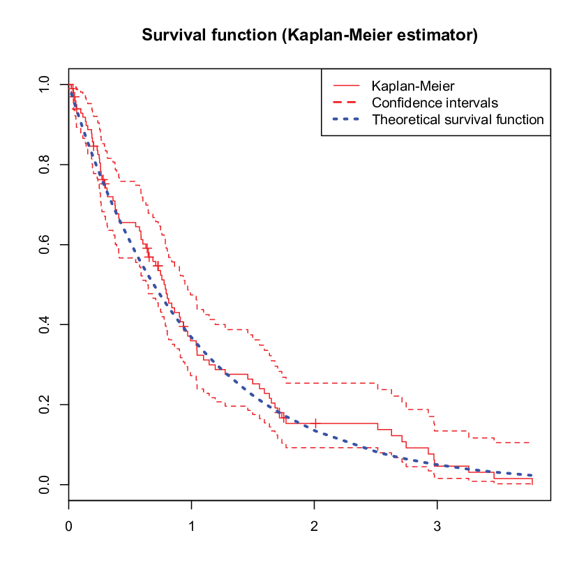
Figure 2 presents the Kaplan-Meier estimator of the survival function for a randomly generated exponential sample $\exp(1)$ of size $100$ with $\exp(1/9)$ as censoring distribution.

In this simulation study we will use the power divergences family Cressie and Read (1984). In this case

Consider the lifetime distribution to be the one parameter exponential $\exp{(\theta)}$ with density $p_{\theta}(x)=\theta e^{-\theta x},~x\geq 0$. The MLE of $\theta_{0}$ is given by

and the AMLE of Oakes (1986) is defined by

It follows that for $\gamma\in\mathbb{R}\setminus\left\{0,1\right\}$

and

For $\gamma=0$,

Observe that this divergence leads to the AMLE, independently upon the value of $\theta$.

For $\gamma=1$,

To make some comparisons, beside dual $\phi$-divergences estimators, we considered minimum density power divergence estimators of Basu et al. (2006), (MDPDE’s), recall that the density power divergence between $g$ and another density $f$ is

The values of $\gamma$ are chosen to be $-1,~0,~0.5,~1,~2$ which corresponds to the well known standard divergences: $\chi_{m}^{2}-$divergence, $KL_{m}$, the Hellinger distance, $KL$ and the $\chi^{2}-$divergence respectively. For the MDPDE’s we take the following values of $\beta:~0.1,~0.5,~1$.

A sample is generated from $\exp(1)$ and $0$, $10$, $25$ of the observations are contaminated by $\exp(5)$ successively. We have used an exponential censoring scheme, the censoring distribution is taken to be $\exp(1/9)$, that the proportion of censoring is $10\%$ . The D$\phi$DE’s $\widehat{\alpha}_{\phi}(\theta)$ are calculated for samples of sizes $25,~50,~75,~100$ and the hole procedure is repeated $1000$ times. The value of escort parameter $\theta$ is taken to be the AMLE. We carried out Kaplan-Meier analysis with the Survival package Therneau and original R port by Thomas Lumley (2009) within the R Language R Development Core Team (2009).

Tables 1 and 2 provide the MSE of various estimates under the model, according to an an increasing proportion of censoring. As expected, when there is no contamination, MLE produces most efficient estimators. A close look at the results of the simulations show that the D$\phi$DE’s performs well under the model, when no outliers are generated. For small sample size $n=25$ and $n=50$, the performance of the estimator under the model is comparable to that of MDPDE’s. Indeed in terms of empirical MSE the D$\phi$DE’s with $\gamma=-1$ produces a lower MSE than the MDPDE’s for all considered values of $\beta$. As $n$ grows up, the MDPDE’s prevail.

Thus, the D$\phi$DE’s are shown to be an attractive alternative to both the AMLE and MDPDE’s in these settings.

References

- Basu and Lindsay (1994) Basu, A. and Lindsay, B. G. (1994). Minimum disparity estimation for continuous models: efficiency, distributions and robustness. Ann. Inst. Statist. Math., 46(4), 683–705.
- Basu et al. (1998) Basu, A., Harris, I. R., Hjort, N. L., and Jones, M. C. (1998). Robust and efficient estimation by minimising a density power divergence. Biometrika, 85(3), 549–559.
- Basu et al. (2006) Basu, S., Basu, A., and Jones, M. C. (2006). Robust and efficient parametric estimation for censored survival data. Ann. Inst. Statist. Math., 58(2), 341–355.
- Bouzebda and Keziou (2010) Bouzebda, S. and Keziou, A. (2010). Estimation and tests of independence in copula models via divergences. Kybernetika, 46(1), 178-201.
- Broniatowski and Keziou (2006) Broniatowski, M. and Keziou, A. (2006). Minimization of -divergences on sets of signed measures. Studia Sci. Math. Hungar., 43(4), 403–442.
- Broniatowski and Keziou (2009) Broniatowski, M. and Keziou, A. (2009). Parametric estimation and tests through divergences and the duality technique. J. Multivariate Anal., 100(1), 16–36.
- Broniatowski and Vajda (2009) Broniatowski, M. and Vajda, I. (2009). Several applications of divergence criteria in continuous families. Technical Report 2257, Academy of Sciences of the Czech Republic, Institute of Information Theory and Automation.
- Cressie and Read (1984) Cressie, N. and Read, T. R. C. (1984). Multinomial goodness-of-fit tests. J. Roy. Statist. Soc. Ser. B, 46(3), 440–464.
- Földes and Rejtő (1981) Földes, A. and Rejtő, L. (1981). A LIL type result for the product limit estimator. Z. Wahrsch. Verw. Gebiete, 56(1), 75–86.
- Hampel et al. (1986) Hampel, F. R., Ronchetti, E. M., Rousseeuw, P. J., and Stahel, W. A. (1986). Robust statistics. Wiley Series in Probability and Mathematical Statistics: Probability and Mathematical Statistics. John Wiley & Sons Inc., New York. The approach based on influence functions.
- Huber (1981) Huber, P. J. (1981). Robust statistics. John Wiley & Sons Inc., New York. Wiley Series in Probability and Mathematical Statistics.
- Jiménez and Shao (2001) Jiménez, R. and Shao, Y. (2001). On robustness and efficiency of minimum divergence estimators. Test, 10(2), 241–248.
- Kaplan and Meier (1958) Kaplan, E. L. and Meier, P. (1958). Nonparametric estimation from incomplete observations. J. Amer. Statist. Assoc., 53, 457–481.
- Keziou (2003) Keziou, A. (2003). Dual representation of -divergences and applications. C. R. Math. Acad. Sci. Paris, 336(10), 857–862.
- Liese and Vajda (1987) Liese, F. and Vajda, I. (1987). Convex statistical distances, volume 95 of Teubner-Texte zur Mathematik [Teubner Texts in Mathematics]. BSB B. G. Teubner Verlagsgesellschaft, Leipzig. With German, French and Russian summaries.
- Liese and Vajda (2006) Liese, F. and Vajda, I. (2006). On divergences and informations in statistics and information theory. IEEE Trans. Inform. Theory, 52(10), 4394–4412.
- Lindsay (1994) Lindsay, B. G. (1994). Efficiency versus robustness: the case for minimum Hellinger distance and related methods. Ann. Statist., 22(2), 1081–1114.
- Maronna et al. (2006) Maronna, R. A., Martin, R. D., and Yohai, V. J. (2006). Robust statistics. Wiley Series in Probability and Statistics. John Wiley & Sons Ltd., Chichester. Theory and methods.
- Miller (1981) Miller, Jr., R. G. (1981). Survival analysis. John Wiley & Sons Inc., New York. With notes by Gail Gong, With problem solutions by Alvaro Mu noz, Wiley Series in Probability and Mathematical Statistics.
- Morales et al. (1995) Morales, D., Pardo, L., and Vajda, I. (1995). Asymptotic divergence of estimates of discrete distributions. J. Statist. Plann. Inference, 48(3), 347–369.
- Oakes (1986) Oakes, D. (1986). An approximate likelihood procedure for censored data. Biometrics, 42(1), 177–182.
- Peterson (1977) Peterson, Jr., A. V. (1977). Expressing the Kaplan-Meier estimator as a function of empirical subsurvival functions. J. Amer. Statist. Assoc., 72(360, part 1), 854–858.
- R Development Core Team (2009) R Development Core Team (2009). R: A Language and Environment for Statistical Computing. R Foundation for Statistical Computing, Vienna, Austria. ISBN 3-900051-07-0.
- Reid (1981) Reid, N. (1981). Influence functions for censored data. Ann. Statist., 9(1), 78–92.
- Stute (1995) Stute, W. (1995). The statistical analysis of Kaplan-Meier integrals. In Analysis of censored data (Pune, 1994/1995), volume 27 of IMS Lecture Notes Monogr. Ser., pages 231–254. Inst. Math. Statist., Hayward, CA.
- Stute (1995a) Stute, W. (1995a). The central limit theorem under random censorship. Ann. Statist., 23(2), 422–439.
- Stute and Wang (1993) Stute, W. and Wang, J.-L. (1993). The strong law under random censorship. Ann. Statist., 21(3), 1591–1607.
- Suzukawa et al. (2001) Suzukawa, A., Imai, H., and Sato, Y. (2001). Kullback-Leibler information consistent estimation for censored data. Ann. Inst. Statist. Math., 53(2), 262–276.
- Therneau and original R port by Thomas Lumley (2009) Therneau, T. and original R port by Thomas Lumley (2009). survival: Survival analysis, including penalised likelihood. R package version 2.35-7.
- Toma and Broniatowski (2010) Toma, A. and Broniatowski, M. (2010). Dual divergence estimators and tests: robustness results. Journal of Multivariate Analysis.
- Wang (1995) Wang, J.-L. (1995). -estimators for censored data: strong consistency. Scand. J. Statist., 22(2), 197–205.
- Wang (1999) Wang, J.-L. (1999). Asymptotic properties of -estimators based on estimating equations and censored data. Scand. J. Statist., 26(2), 297–318.
- Welsh (1989) Welsh, A. H. (1989). On -processes and -estimation. Ann. Statist., 17(1), 337–361.
- Yang (1991) Yang, S. (1991). Minimum Hellinger distance estimation of parameter in the random censorship model. Ann. Statist., 19(2), 579–602.
- Ying (1992) Ying, Z. (1992). Minimum Hellinger-type distance estimation for censored data. Ann. Statist., 20(3), 1361–1390.