1Introduction

1 Introduction

The Truncated Conformal Space approach (TCSA) of Yurov and Zamolodchikov [1] has been a widely-used method to study the finite-size dependence of perturbed two-dimensional conformal field theories for quite some time [2, 3, 4, 5, 6, 7, 8]. It is based on truncating the infinite dimensional Hilbert space to a finite-dimensional system on which the Hamiltonian is studied numerically.¹¹ 1 In this paper we study the original form due to Yurov and Zamolodchikov, not the revised version of [9, 10]. It has been known for a long time that the method has various convergence problems which can reduce its effectiveness [2, 3]. The principal problems that have been noted before are the divergence of, and differences between ground state contributions in different sectors. Once these have been taken into account by considering only differences of energy levels in the same sector, the effects of truncation can still be important. There has been some interesting work on extrapolation in truncation level [4, 5], assuming an underlying but unknown scaling behaviour. Here, we conjecture that the most important corrections after the ground state divergence are a renormalisation of the coupling constant and a renormalisation of the energy scale. Our main results are perturbative expressions for the leading coupling-constant and energy-scale renormalisations. We apply these to the tri-critical Ising model as considered in both [2] and [3] and show that the behaviour of the TCSA results is greatly improved. We also find numerical results for the renormalisation and rescaling for the tri-critical Ising model and show that the TCSA approach remains very accurate even when these two effects become large.

One important result we find is that while the TCSA estimates of energy gaps converge for perturbations with conformal weight less than $3/4$ , they do not for those with weight greater than $3/4$ . We show this in the case of the minimal model $M_{9,10}$ perturbed by a field of weight $4/5$ . This failure of convergence is entirely due to the divergence of the energy rescaling; once the energy rescaling is taken into account the TCSA estimates converge as well as before. In other words, the TCSA estimates of ratios of energy gaps converge even if the gaps themselves do not.

The paper is organised as follows. We first introduce the TCSA approximation and present the problems to be addressed in section 2. We then discuss the perturbative results for the coupling-constant and energy renormalisations in sections 3 and 4, and present the results for the models considered in [2] and [3] in sections 5.1 and 5.3. In section 6 we then discuss the problems occurring with $h>3/4$ and in section 7 the complications for perturbed models on the strip.

2 The TCSA approach and its errors

2.1 The TCSA approach to bulk perturbations

At present, the TCSA can be applied to bulk perturbations in two different arenas: when the model is defined on a circle and when it is defined on a strip. The original paper of Yurov and Zamolodchikov [1] treats the cylinder case, the boundary case was initiated in [11]. We consider here the case of the cylinder, and defer the strip to section 7.

We start with a CFT defined on a cylinder of circumference $R$ which we take to be a strip $0\leq y<R$ of width $R$ in the complex plane with coordinate $z=x+iy$ , and with the two edges of this strip identified. For the details of CFT, see [12].

The unperturbed Hamiltonian generating translations along the cylinder is

H=\int_{0}^{R}T_{xx}\;\frac{{\mathrm{d}}y}{2\pi}\;.

(2.1)

We will map the strip to the complex plane with coordinate $w=\exp(2\pi z/R)$ in terms of which the CFT Hamiltonian is

H=\frac{2\pi}{R}\left(L_{0}+\bar{L}_{0}-\frac{c}{12}\right)\;,

(2.2)

where $L_{0}$ and $\bar{L}_{0}$ are the zero modes of the two copies of the Virasoro algebra present in the theory defined on a plane.

We are interested in perturbations by one or more bulk fields $\varphi_{i}(x,y)$ . We take these to be spinless quasi-primary fields of equal left and right conformal dimensions $(h_{i},h_{i})$ . If the coupling to these fields are $\mu_{i}$ then the perturbation is given by an addition to the action

\delta S=\int\sum_{i}\mu_{i}\varphi_{i}(x)\,{\mathrm{d}}^{2}x\;.

(2.3)

When mapped to the upper half plane this gives the perturbation to the Hamiltonian as

\delta H=\sum_{i}\mu_{i}\left(\frac{R}{2\pi}\right)^{1-2h_{i}}\,\int_{\theta=0}^{2\pi}\varphi_{i}(e^{i\theta})\,{\mathrm{d}}\theta\;,

(2.4)

where $w=r\exp(i\theta)$ so that $y=(2\pi\,\theta/R)$ .

Since the circle has rotational symmetry, one can restrict attention to the rotationally invariant states on which $L_{0}-\bar{L}_{0}=0$ . On these states, we can perform the $\theta$ –integral in (2.4) so that the perturbed Hamiltonian becomes

H=\frac{2\pi}{R}\left[L_{0}+\bar{L}_{0}-\tfrac{c}{12}+\sum_{i}(2\pi)^{1-y_{i}}\lambda_{i}\,\varphi_{i}(1).\right]\;,

(2.5)

where $y_{i}=2-2h_{i}$ and $\lambda_{i}=\mu_{i}R^{y_{i}}$ are dimensionless coupling constants. This is the TCSA Hamiltonian of [1].

The TCSA method is to truncate the Hilbert space in some prescribed manner and take the Hamiltonian to be (2.5) on the truncated space. There are at least two ways this has been implemented.

2.1.1 Truncation by level

The first method is to truncate the space to level $n$ in each representation in the Hilbert space, as in [1]. This means that the maximum value of $L_{0}+\bar{L}_{0}$ in each representation is $(2n+h_{i}+\bar{h}_{i})$ . This can cause problems if the Hilbert space includes some representations with large values of $h$ , as these high level states cause distinct qualitative changes to the spectrum.

2.1.2 Truncation by total energy

The second method is to truncate so that $L_{0}+\bar{L}_{0}\leq 2n$ ; this means that the maximum value of $L_{0}+\bar{L}_{0}$ in each representation is $2n$ , and so if a representation has $h>n$ , it will be completed excluded from the TCSA space at level $n$ . This method has the advantage that high weight representations do not unduly affect the TCSA space, that the space at level $n$ is smaller than in the truncation by level, but has the disadvantage that the truncation affects are harder to deal with analytically.

These two methods will give very similar results when $n\gg h$ for all $h$ in a particular model. It is worth pointing out that choosing a different truncation method can have dramatic effects – the “mode truncation” investigated by Tóth in [14] has a very different behaviour. We shall use the level truncation unless stated otherwise.

The operator $H$ in (2.5) is dimensionful, and it is far preferable to work with dimensionless operators, or dimensionless eigenvalues. In the case of bulk perturbations, there are two natural choices.

2.1.3 Flows ending in massless theories

If the IR limit of the flow is a massless theory, then it is natural to work with the scaling functions defined in terms of the energy eigenvalues $E_{n}$ as

e_{n}(\lambda_{i})=\left(\frac{R}{2\pi}\right)E_{n}(\lambda_{i})\;,

(2.6)

The scaling functions are expected to flow to the eigenvalues of the operator

\left(L_{0}+\bar{L}_{0}-\tfrac{c}{12}\right)_{IR}\;,

(2.7)

at the IR fixed point with a correspondingly simple spectrum.

2.1.4 flows ending in massive theories

If the IR limit of the flow is a massive theory, then the mass of the lightest stable particle, $m$ , gives a natural scale and one considers the dimensionless operator

\frac{H}{m}=\frac{2\pi}{r}\left[L_{0}+\bar{L}_{0}-\tfrac{c}{12}+\sum_{i}(2\pi)^{1-y_{i}}\frac{\lambda_{i}}{m^{y_{i}}}r^{y_{i}}\,\varphi_{i}(1).\right]\;,

(2.8)

where $r=mR$ is a dimensionless variable and $\lambda_{i}m^{-y_{i}}$ are a set of numbers.

2.1.5 Problems with the TCSA

The original model studied with the TCSA by Yurov and Zamolodchikov was the Lee-Yang model perturbed by its primary field $\varphi_{(1,3)}$ of weight $h=-1/5$ . The results in this model, whether as in the original case on the cylinder [1], or on the strip [11], have been exceptionally accurate, up to 14 digits for some quantities. When the TCSA method was applied more generally in [2] and [3], it was clear that this was not always the case. There were several problems identified in [2] for the perturbation of the tri-critical Ising model by the primary field of weight $3/5$ ; we discuss these problems in turn.

The first is that the Hilbert space of the model may split up into several sectors and the TCSA eigenvalues in these sectors may differ by unphysical amounts. In our prototypical examples of perturbations by $\varphi_{13}$ and $\varphi_{31}$ , the perturbation will only couple together representations in the same row or same column of the Kac table. For example, the tri-critical Ising model has representations $\{(r,s);1\leq r\leq 3,1\leq s\leq 4,r+s\,\mathrm{even}\}$ . Under the action of $\varphi_{(1,3)}$ these fall into three sectors which we denote $(r,*)$ for $r=1,2$ and $3$ . Under the action of $\varphi_{(3,1)}$ , they split into four sectors, which we denote $(*,r)$ for $r=1,2,3$ and $4$ . Under the massless flow generated by $\varphi_{(1,3)}$ , the $(*,r)$ sector flows into the $(1,r)$ representation of the Ising model. Under the massive flow generated by $\varphi_{(1,3)}$ , the three sectors flow into three sectors of the massive model, corresponding to the splitting of the three degenerate ground states of the massive kink model. Under the irrelevant flow generated by $\varphi_{(3,1)}$ , the $(*,r)$ sector flows into the corresponding $(r,*)$ sector of the minimal model $M(5,6)$ . The problem is that the TCSA gives slightly different results for the ground state energy is the different sectors, so that it may be impossible to get accurate results for energy differences of states in different sectors. Sometimes interpolation in truncation level or size of the truncated space produces sensible results, as was reported in [18]. The main result we have to report is that the energy rescaling formula we find in section 4 is slightly different in different representations, and that this effect is most noticeable for the ground states in each sector. This greatly improves the difference between the ground states in the different sectors, as can be seen in figure 5.

Secondly, if the weight of the perturbing field becomes larger than 1/2, the conformal perturbation expansion and correspondingly the TCSA eigenvalues, become divergent. This has the result that the ground state energy of the TCSA system does not converge with increasing truncation level. This was observed in [2] and discussed in [20]. It was realised that this divergence can arise purely from the second order contribution for which there is an exact expression. Subtracting the divergent part of this expression then gives a revised TCSA estimate which will converge, with increasing truncation level, to the perturbed conformal field theory result, as observed by Takács [21]. We re-derive this leading term as part of our treatment of the energy rescaling in section 4. We illustrate the effectiveness of these subtractions in the case of the massless perturbation of the tri-critical Ising model considered in [2]. We show in figure 1(b) that this works well in the case of the tri-critical Ising model perturbation considered problematic in [2] - after subtraction of the leading divergence, the ground state energy does then converge for this perturbation.

Finally, it also appears that the “scaling region” is not easily reached, the region where the eigenvalues scale with truncation level in the expected manner. Our solution is that suggested in [2], a careful consideration of the scaling of the model with system size which we show reduces, in the cases considered in [2], to a renormalisation of the coupling constant and a representation-dependent re-scaling of the Hamiltonian. This is almost the same as we found in [16]. As in [16], perturbative expansions for these effects can be found by considering the change in the energy eigenvalues with truncation level. We consider first the coupling constant renormalisation in section 3, and then the ground state energy and energy rescaling in section 4 and apply them to the tri-critical Ising model in section 5.

3 Coupling constant renormalisation

The derivation of the coupling constant renormalisation is a straightforward generalisation of the boundary case. We assume that the perturbed correlation functions on the cylinder with coordinates $(x,y)$ are given by the insertion of the expression

\mathcal{P}\exp\left(-\sum_{i}\mu_{i}\int_{x=-\infty}^{\infty}\int_{y=0}^{R}P_{n}\,\varphi_{i}(x,y)_{cyl}\,P_{n}\;{\mathrm{d}}y{\mathrm{d}}x\right)\;,

(3.1)

in the unperturbed expressions, where $\mathcal{P}$ denotes path ordering and $P_{n}$ denotes the projector onto states at level $n$ or lower. After mapping to the plane with $w=exp(2\pi z/R)$ , $r=\exp(2\pi x/R)$ , $\theta=2\pi y/R$ , this becomes

			$\displaystyle\mathcal{P}\exp\left(-\sum_{i}\lambda_{i}(2\pi)^{-y_{i}}\int_{r=0}^{\infty}\int_{\theta=0}^{2\pi}P_{n}\,\varphi_{i}(w,\bar{w})_{cyl.}\,P_{n}\;\frac{r{\mathrm{d}}r{\mathrm{d}}\theta}{r^{y_{i}}}\right)$		(3.2)
		$\displaystyle=$	$\displaystyle 1-\sum_{i}\tilde{\lambda}_{i}\int_{r=0}^{\infty}\int_{\theta=0}^{2\pi}P_{n}\,\varphi_{i}(w,\bar{w})_{cyl.}\,P_{n}\;\frac{{\mathrm{d}}r{\mathrm{d}}\theta}{r^{y_{i}-1}}+\ldots\;,$		(3.2)

where $y_{i}=2-2h_{i}$ and $\tilde{\lambda}_{i}=(2\pi)^{-y_{i}}\lambda_{i}$ is introduced for convenience. We require that the perturbed correlation functions be invariant when the truncation level $n$ is changed. The simplest way to find the leading order change in the coupling constants is to consider the matrix elements of the integrand of $\int_{0}^{\infty}r^{1-y}{\mathrm{d}}r$ in (3.2) taken at $r=1$ and taken in the states ${\langle{\varphi_{i}}|}\ldots{{|{0}\rangle}}$ , that is we consider

Z_{i,n}=-(2\pi)\tilde{\lambda}_{i}+\sum_{j,k}(2\pi)\tilde{\lambda}_{j}\tilde{\lambda}_{k}\int_{r=0}^{1}\int_{\theta=0}^{2\pi}{\langle{\varphi_{i}}|}\varphi_{j}(1,1)P_{n}\varphi_{k}(r,\theta){{|{0}\rangle}}\frac{{\mathrm{d}}r{\mathrm{d}}\theta}{r^{y_{k}-1}}+\ldots\;,

(3.3)

where we have performed one of the angular integrations. We have also used the first of the properties of the primary fields

	$\displaystyle{\langle{\varphi_{i}}\|}\varphi_{j}(w,\bar{w}){{\|{0}\rangle}}$	$\displaystyle=$	$\displaystyle\delta_{ij}\|w\|^{-2h_{i}}\;,$
	$\displaystyle{\langle{\varphi_{i}}\|}\varphi_{j}(1,1)\varphi_{k}(w,\bar{w}){{\|{0}\rangle}}$	$\displaystyle=$	$\displaystyle\frac{C_{ijk}}{\|1-w\|^{2(h_{i}-h_{j}-h_{k})}}$		(3.4)

Requiring $Z_{i,n}=Z_{i,n-1}$ , we find

\tilde{\lambda}_{i}(n)-\tilde{\lambda}_{i}(n-1)=\sum_{j,k}\tilde{\lambda}_{j}\tilde{\lambda}_{k}\int_{r=0}^{1}\int_{\theta=0}^{2\pi}{\langle{\varphi_{i}}|}\varphi_{j}(1,1)\left[P_{n}-P_{n-1}\right]\varphi_{k}(r,\theta)\,{{|{0}\rangle}}\frac{{\mathrm{d}}r{\mathrm{d}}\theta}{r^{y_{k}-1}}\;.

(3.5)

From (3.4),

\int_{0}^{2\pi}{\langle{\varphi_{i}}|}\varphi_{j}(1,1)\left[P_{n}-P_{n-1}\right]\varphi_{k}(r,\theta)\,{{|{0}\rangle}}{\mathrm{d}}\theta=2\pi C_{ijk}\left[\frac{\Gamma(h_{j}+h_{k}-h_{i}+n)}{\Gamma(h_{j}+h_{k}-h_{i})\Gamma(n+1)}\right]^{2}\,r^{2n}\;.

(3.6)

Substituting (3.6) in (3.5), performing the $r$ integral and expanding out to leading order in $n$ , we get

n\frac{{\mathrm{d}}\tilde{\lambda}_{i}}{{\mathrm{d}}n}\simeq n(\tilde{\lambda}_{i}(n)-\tilde{\lambda}_{i}(n-1))\simeq\sum_{jk}n^{y_{i}-y_{j}-y_{k}}\tilde{\lambda}_{j}\tilde{\lambda}_{k}\frac{2\pi C_{ijk}}{\Gamma(h_{j}+h_{k}-h_{i})^{2}}\;.

(3.7)

As we see, there are corrections to $\lambda_{i}$ from all pairs of fields $\varphi_{j}$ , $\varphi_{k}$ which couple to $\varphi_{i}$ , but that those for which $h_{i}-h_{j}-h_{k}>0$ , i.e. those which appear in the regular part of the operator product expansion, do not give important corrections. In the simplest case where we consider the perturbation by a single field where the only primary fields occurring in the singular part of its operator product expansion are the identity and the field itself, this gives for $\lambda(n)$ ,

n\frac{{\mathrm{d}}\lambda}{{\mathrm{d}}n}=\frac{\lambda^{2}}{(2\pi n)^{y}}\frac{2\pi C}{\Gamma(h)^{2}}+O(\lambda^{3})\;,

(3.8)

where $C$ is the three-point coupling. If $y>0$ , this can be integrated to find the effective “exact” coupling $\lambda_{\infty}$ in terms of the TCSA coupling $\lambda(n)$ at level $n$ :

\lambda_{\infty}=\frac{\lambda(n)}{1-\frac{2\pi C}{y\Gamma(h)^{2}}\frac{\lambda(n)}{(2\pi n)^{y}}}+O(\lambda^{3})\;,\;\;\;\;\lambda(n)=\frac{\lambda_{\infty}}{1+\frac{2\pi C}{y\Gamma(h)^{2}}\frac{\lambda_{\infty}}{(2\pi n)^{y}}}+O(\lambda^{3})\;.

(3.9)

This is our one-loop prediction for the coupling constant renormalisation. As we see below, this can be improved to take into account the level $m$ of the unperturbed state which leads to the replacement of $n$ by $n-m$ in (3.9).

4 The ground-state divergence and the energy rescaling

4.1 Perturbation theory results

As in [16], the energy rescaling arises as the sub-leading correction to the coupling to the identity operator. The bulk case is not as clear-cut as the boundary case, however, as the presence of multiple internal channels means that there are small differences in the rescaling for states that arise from different representations. We shall also see that the rescaling does not necessarily go to zero for all renormalisable perturbations, and for the perturbation by a single field, it diverges with $n$ if $h>3/4$ . We find these corrections by evaluating the eigenvalues of the perturbed Hamiltonian to second order.

We consider the simplest case of the perturbation by a single field $\varphi$ of weight $h$ with coupling $\lambda$ and the scaling operator

\hat{h}=(L_{0}+\bar{L}_{0}-\tfrac{c}{12})+\sum_{i}\tilde{\lambda}_{i}\int_{\theta=0}^{2\pi}\varphi_{i}(e^{i\theta})\,\frac{{\mathrm{d}}\theta}{2\pi}\;,

(4.1)

where, again, $\tilde{\lambda}=(2\pi)^{-y}\lambda$ . The eigenvalues of $\hat{h}$ are the scaling functions and we denote the $i$ -th eigenvalue by $e_{i}$ and take its expansion to be

e_{i}(\lambda)=\sum e_{i,m}\;\tilde{\lambda}^{m}\;,

(4.2)

If $h\geq 1/2$ then one or more of these coefficients will formally be divergent. For example, if the unperturbed state ${|{i}\rangle}$ is a highest weight state then the first three coefficients are

	$\displaystyle e_{i,0}=(2h_{i}-\tfrac{c}{12})\;,\;\;e_{i,1}=2\pi C_{i\varphi i}\;,\;\;$		(4.3)
	$\displaystyle e_{i,2}=-2\pi\int_{\|z\|<1}\frac{{\mathrm{d}}^{2}z}{\|z\|^{y}}\left({\langle{i}\|}\varphi(1)\varphi(z){\|{i}\rangle}-\frac{(C_{i\varphi i})^{2}}{\|z\|^{2h}}\right)\;.$		(4.4)

For all states except the the vacuum, ${|{i}\rangle}={{|{0}\rangle}}$ , the integral in $e_{i,2}$ depends in detail on the model in question but is divergent if $h\geq 1/2$ . For the vacuum case with $h<1/2$ , the third and fourth coefficients are given in [20] as²² 2 Note that these differ by powers of $(2\pi)^{y}$ as [20] uses the expansion parameter $\lambda$ , not $\tilde{\lambda}$ .

e^{A}_{0,2}=-\tfrac{1}{4}(2\pi)^{2}\gamma^{2}(1-\tfrac{y}{2})\gamma(y-1)\;,\;\;e^{A}_{0,3}=\frac{(2\pi)^{3}}{48}\gamma^{3}(\tfrac{1}{2}-\tfrac{1}{4})\gamma(\tfrac{3y}{4}-\tfrac{1}{2})C_{\varphi\varphi\varphi}\;,

(4.5)

where $\gamma(x)=\Gamma(x)/\Gamma(1-x)$ and $A$ denotes the analytic expression. The expressions (4.5) can be analytically continued to $h>1/2$ and then agree with the coefficients in the corresponding TBA calculation. As pointed out in [20], the TCSA method does not reproduce the analytically continued expressions but instead approximates the divergent expression (4.4). We now demonstrate how we calculate these terms.

4.2 TCSA results

The first truncation effects arise in the coefficients $e_{i,2}$ . We shall denote the contribution to $e_{i,m}$ from the states at TCSA truncation level $n$ by $e_{i,m}^{[n]}$ and the full coefficient in the exact TCSA expansion at truncation level $n$ by $e_{i,m}^{n}$ , so that the TCSA approximation to $e_{i}(\lambda)$ is

e_{i}^{n}(\lambda)=\sum_{m}e_{i,m}^{n}\,\tilde{\lambda}^{m}\;,\;\;\;\;e_{i,m}^{n}=\sum_{k=0}^{n}e_{i,m}^{[k]}\;.

(4.6)

The term $e_{i,2}^{[n]}$ comes from level $n$ intermediate states in the four-point function ${\langle{i}|}\varphi(1)\varphi(z){|{i}\rangle}$ . In the boundary situation in [16] we could arrange the boundary conditions so that the four point function in that calculation was given by a single chiral block; in the bulk this is not possible. Instead, we expand the four point function in (4.4) over the set of chiral blocks³³ 3 See [12] for details as

{\langle{i}|}\varphi(1)\varphi(z){|{i}\rangle}=\sum_{j}(C_{i\varphi j})^{2}\left|{\hbox to102.43008pt{\raise-5.69054pt\vbox{\begin{picture}(4301.0,-2463.0){\put(4800.0,-1960.0){\line{ 0}{-1}{500.0}}}{\put(5700.0,-1960.0){\line{ 0}{-1}{500.0}}}{\put(4250.0,-2460.0){\line{ 1}{ 0}{2000.0}}}\put(4200.0,-2460.0){\pic@makebox@{\makebox}{}(0.0,0.0)[rc]{$i$}}\put(4800.0,-1900.0){\pic@makebox@{\makebox}{}(0.0,0.0)[cb]{$\varphi$}}\put(4800.0,-2560.0){\pic@makebox@{\makebox}{}(0.0,0.0)[ct]{$1$}}\put(5250.0,-2380.0){\pic@makebox@{\makebox}{}(0.0,0.0)[cb]{$j$}}\put(5700.0,-1900.0){\pic@makebox@{\makebox}{}(0.0,0.0)[cb]{$\varphi$}}\put(5700.0,-2560.0){\pic@makebox@{\makebox}{}(0.0,0.0)[ct]{$z$}}\put(6350.0,-2460.0){\pic@makebox@{\makebox}{}(0.0,0.0)[lc]{$i$}}\end{picture}}}}\right|^{2}\;.

(4.7)

The contribution from the states at level $n$ in the $j$ intermediate channel comes from the coefficient of $z^{n-h_{{i}}-h+h_{j}}$ . As in [16], we find the leading $n$ -dependence of this coefficient by expanding the conformal block in powers of $(1-z)$ ,

		$\displaystyle=$	$\displaystyle\sum_{k}F_{jk}\cdot{\hbox to79.6678pt{\raise-5.69054pt\vbox{\begin{picture}(4600.0,-2483.0){\put(4850.0,-1860.0){\line{ 1}{0}{800.0}}}{\put(4850.0,-2460.0){\line{ 1}{0}{800.0}}}{\put(5250.0,-1860.0){\line{ 0}{-1}{600.0}}}\put(4775.0,-2460.0){\pic@makebox@{\makebox}{}(0.0,0.0)[rc]{${i}$}}\put(4775.0,-1860.0){\pic@makebox@{\makebox}{}(0.0,0.0)[rc]{$\varphi(1)$}}\put(5750.0,-1860.0){\pic@makebox@{\makebox}{}(0.0,0.0)[lc]{$\varphi(z)$}}\put(5750.0,-2460.0){\pic@makebox@{\makebox}{}(0.0,0.0)[lc]{${i}$}}\put(5300.0,-2160.0){\pic@makebox@{\makebox}{}(0.0,0.0)[lc]{$k$}}\end{picture}}}}$		(4.8)
		$\displaystyle=$	$\displaystyle F^{i}_{j1}\cdot{\hbox to79.6678pt{\raise-5.69054pt\vbox{\begin{picture}(4600.0,-2483.0){\put(4850.0,-1860.0){\line{ 1}{0}{800.0}}}{\put(4850.0,-2460.0){\line{ 1}{0}{800.0}}}{\put(5250.0,-1860.0){\line{ 0}{-1}{600.0}}}\put(4775.0,-2460.0){\pic@makebox@{\makebox}{}(0.0,0.0)[rc]{${i}$}}\put(4775.0,-1860.0){\pic@makebox@{\makebox}{}(0.0,0.0)[rc]{$\varphi(1)$}}\put(5750.0,-1860.0){\pic@makebox@{\makebox}{}(0.0,0.0)[lc]{$\varphi(z)$}}\put(5750.0,-2460.0){\pic@makebox@{\makebox}{}(0.0,0.0)[lc]{${i}$}}\put(5300.0,-2160.0){\pic@makebox@{\makebox}{}(0.0,0.0)[lc]{$1$}}\end{picture}}}}+F^{i}_{j\varphi}\cdot{\hbox to79.6678pt{\raise-5.69054pt\vbox{\begin{picture}(4600.0,-2483.0){\put(4850.0,-1860.0){\line{ 1}{0}{800.0}}}{\put(4850.0,-2460.0){\line{ 1}{0}{800.0}}}{\put(5250.0,-1860.0){\line{ 0}{-1}{600.0}}}\put(4775.0,-2460.0){\pic@makebox@{\makebox}{}(0.0,0.0)[rc]{${i}$}}\put(4775.0,-1860.0){\pic@makebox@{\makebox}{}(0.0,0.0)[rc]{$\varphi(1)$}}\put(5750.0,-1860.0){\pic@makebox@{\makebox}{}(0.0,0.0)[lc]{$\varphi(z)$}}\put(5750.0,-2460.0){\pic@makebox@{\makebox}{}(0.0,0.0)[lc]{${i}$}}\put(5300.0,-2160.0){\pic@makebox@{\makebox}{}(0.0,0.0)[lc]{$\varphi$}}\end{picture}}}}+\ldots\;,$		(4.9)

where $F^{i}_{jk}=F_{jk}[{{\varphi\varphi}\atop{ii}}]$ are the crossing matrix elements and

		$\displaystyle=$	$\displaystyle(1-z)^{-2h}\left(1+\tfrac{2h^{2}}{c}(1-z)^{2}+O(1-z)^{3}\right)\;,\;\;$
		$\displaystyle=$	$\displaystyle(1-z)^{-h}\left(1+\tfrac{h}{2}(1-z)+O(1-z)^{2}\right)\;.$		(4.10)

We have assumed that the identity and $\varphi$ are the most singular fields in the operator product $\varphi*\varphi$ ; if not, there will be correspondingly more terms in (4.9). Hence we find the leading terms arising at truncation level $n$ in the chiral block are

					(4.11)
		$\displaystyle=$	$\displaystyle z^{n-h_{i}-h+h_{j}}\left(\frac{F^{i}_{j1}\Gamma(n{-}h_{i}{+}h_{j}{+}h)}{\Gamma(2h)\Gamma(n{-}h_{i}{+}h_{j}{-}h{+}1)}+\frac{F^{i}_{j\varphi}\Gamma(n{-}h_{i}{+}h_{j})}{\Gamma(2h)\Gamma(n{-}h_{i}{+}h_{j}{-}h{+}1)}+\ldots\right)$		(4.11)

This gives the second order truncation level $n$ contribution to the energy as

$\displaystyle e^{[n]}_{i,2}$	$\displaystyle{=}$	$\displaystyle-2\pi\sum_{j}\frac{(C_{{i}\varphi j})^{2}}{2(n{-}h_{i}{+}h_{j})\Gamma(n{-}h_{i}{-}h{+}h_{j}{+}1)^{2}}$	(4.12)
		$\displaystyle\qquad\qquad\qquad\qquad{}\times\left[F^{i}_{j1}\frac{\Gamma(n{-}h_{i}{+}h{+}h_{j})}{\Gamma(2h)}+F^{i}_{j\varphi}\frac{\Gamma(n{-}h_{i}{+}h_{j})}{\Gamma(h)}+\ldots\right]^{2}$
	$\displaystyle{=}$	$\displaystyle-2\pi\sum_{j}(C_{{i}\varphi j})^{2}\Big[n^{4h{-}3}\frac{(F^{i}_{j1})^{2}}{2\Gamma(2h)^{2}}+n^{4h{-}4}(4h-3)\frac{(F^{i}_{j1})^{2}(h_{j}{-}h_{i})}{2\Gamma(2h)^{2}}$
		$\displaystyle\qquad\qquad{}+n^{3h{-}3}\frac{F^{i}_{j1}F^{i}_{j\varphi}}{\Gamma(h)\Gamma(2h)}+n^{2h{-}3}\frac{(F^{i}_{j\varphi})^{2}}{2\Gamma(h)}+O(n^{4h{-}5},n^{3h{-}4},n^{2h{-}4})\Big]\;.$

Using the crossing properties of the full correlation functions, we find

\sum_{j}(F^{i}_{j1}C_{{i}\varphi j})^{2}=1\;,\;\;\sum_{j}(F^{i}_{j\varphi}C_{{i}\varphi j})^{2}=C_{\varphi\varphi\varphi}C_{{i}{i}\varphi}\;,\;\;\sum_{j}F^{i}_{j1}F^{i}_{j\varphi}(C_{{i}\varphi j})^{2}=0\;,

(4.13)

so that the second order truncation level $n$ contributions (4.12) are

e_{i,2}^{[n]}=-2\pi\Big[\frac{n^{4h{-}3}}{2\Gamma(2h)^{2}}+(4h-3)\frac{(\alpha_{i}{-}h_{i})n^{4h{-}4}}{2\Gamma(2h)^{2}}+\frac{C_{\varphi\varphi\varphi}C_{{i}{i}\varphi}}{2\Gamma(h)}n^{2h{-}3}+O(n^{4h{-}5},n^{3h{-}4},n^{2h{-}4})\;\Big]\;,

e_{0,2}^{[n]}=-2\pi\Big[\frac{n^{4h{-}3}}{2\Gamma(2h)^{2}}+(4h-3)\frac{hn^{4h{-}4}}{2\Gamma(2h)^{2}}+O(n^{4h{-}5},n^{3h{-}4},n^{2h{-}4})\;\Big]\;,

(4.14)

where

\alpha_{i}=\sum_{j}h_{j}(C_{{i}\varphi j}F^{i}_{j1})^{2}=\frac{S_{11}}{S_{1\varphi}}\sum_{j\in i*\varphi}\frac{S_{1j}}{S_{1i}}h_{j}\;,\;\;\alpha_{0}=h\;,

(4.15)

where the second expression in the modular S-matrix $S_{ij}$ holds for a diagonal modular invariant [17]. If ${|{i}\rangle}$ is a highest weight state then we can then sum these contributions to get

	$\displaystyle e_{0,2}^{n}$	$\displaystyle=$	$\displaystyle e_{0,2}^{A}-2\pi\left[\frac{n^{4h-2}}{4(2h-1)\Gamma(2h)^{2}}+\frac{n^{4h-3}}{\Gamma(2h)^{2}}\frac{2h{+}1}{4}+\ldots\right]\;,$		(4.16)
	$\displaystyle e_{i,2}^{n}$	$\displaystyle=$	$\displaystyle e_{i,2}^{A}-2\pi\left[\frac{n^{4h-2}}{4(2h-1)\Gamma(2h)^{2}}+\frac{n^{4h-3}}{\Gamma(2h)^{2}}\frac{2(\alpha_{i}{-}h_{i}){+}1}{4}+\frac{C_{ii\varphi}C_{\varphi\varphi\varphi}n^{2h-2}}{2(2h-2)\Gamma(h)^{2}}+\ldots\right]\;.$

If the TCSA coefficients are convergent, then (4.16) gives the leading corrections; if they are divergent, they give the leading divergences. We first consider this result for the ground state scaling function.

For $h>1/2$ , the leading term(s) in (4.16) are divergent. To get a proper estimate of the ground state energy from TCSA we need explicitly to subtract these. We do this for the divergent case considered in [2] in section 5.1. As will be seen, this is very effective at producing a good estimate from the TCSA.

For excited states, we shall only consider the scaled energy gap, $\tilde{e}_{i}=e_{i}-e_{0}=\sum\tilde{e}_{i,k}\tilde{\lambda}^{k}$ and its TCSA approximation $\tilde{e}^{n}_{i}=\sum\tilde{e}^{n}_{i,k}\tilde{\lambda}^{k}$ . Using (4.16), we can write the TCSA approximation as

$\displaystyle\tilde{e}_{i}^{n}(\lambda)$	$\displaystyle=$	$\displaystyle(2h_{i})+(2\pi)\tilde{\lambda}C_{i\varphi i}+\tilde{\lambda}^{2}\left(\tilde{e}^{A}_{i,2}+2\pi\frac{n^{1-2y}}{\Gamma(2h)^{2}}\frac{h_{i}-\delta_{i}}{2}+2\pi C_{ii\varphi}C_{\varphi\varphi\varphi}\frac{n^{-y}}{2y\Gamma(h)^{2}}\right)$	(4.17)
	$\displaystyle=$	$\displaystyle 2\delta_{i}{+}\left(1{+}\frac{2\pi\tilde{\lambda}^{2}}{4\Gamma(2h)^{2}n^{2y-1}}\right)\left(2(h_{i}{-}\delta_{i}){+}(2\pi)\left(\tilde{\lambda}+\frac{\tilde{\lambda}^{2}C_{\varphi\varphi\varphi}}{2y\Gamma(h)^{2}n^{y}}\right)C_{i\varphi i}+\tilde{e}^{A}_{0,2}\tilde{\lambda}^{2}\right){+}\ldots$
	$\displaystyle=$	$\displaystyle r_{n}^{i}(\lambda)\;\left[\tilde{e}_{i}(\lambda g_{n}(\lambda))-2\delta_{i}\right]+2\delta_{i}\;+\;O(\lambda^{3})\;,$

where $\delta_{i}=\alpha_{i}-h_{i}$ . which defines the one-loop energy rescaling $r_{n}^{i}$ and coupling constant renormalisation $g_{n}(\lambda)$ ,

r^{i}_{n}(\lambda)=\left(1+\frac{\lambda^{2}}{4\Gamma(2h)^{2}(2\pi n)^{2y-1}}\right)\;,\;\;g_{n}(\lambda)=\left(1+\frac{\lambda\,C}{2y\Gamma(h)^{2}(2\pi n)^{y}}\right)\;.

(4.18)

The coupling constant renormalisation agrees perfectly with the result of the previous section, (3.9). The energy rescaling is a new prediction. It differs from the boundary case as the energy rescaling is not exactly the same for each state, because there is at this order a small shift $\delta_{i}$ which differs between states arising in different representations. Since this is a small overall constant shift in each representation, it is only important for the lowest lying states in each representation where it does make a noticeable difference, as we see in the plots in section 5.3.

These results also hold, suitably adjusted, for excited states. If ${|{\psi}\rangle}$ is a state at level $m$ in the representation $i$ then the contribution in (4.7) from the intermediate states at level $n$ comes from the coefficient of $z^{n-(h_{{i}}+m)-h+h_{j}}$ and following the changes through the net result is to replace $n$ in (4.18) by $(n-m)$ , so that for the state ${|{\psi}\rangle}$ the rescaling and renormalisation are

r^{\psi}_{n}(\lambda)=\left(1+\frac{\lambda^{2}}{4\Gamma(2h)^{2}(2\pi(n-m))^{2y-1}}\right)\;,\;\;g_{n}^{\psi}(\lambda)=\left(1+\frac{\lambda\,C}{2y\Gamma(h)^{2}(2\pi(n-m))^{y}}\right)\;.

(4.19)

This alteration is a sub-leading effect in $n$ but is appreciable for the cases we consider when $n$ is sometimes quite small.

5 Tests of the TCSA in the tri-critical Ising model

One of the first paper to use the TCSA extensively was [2]. This investigated perturbations of the tri-critical Ising model with mixed success. With hindsight, it is easy to see now why they obtained good results for the perturbations by the fields of weight $1/10$ and $3/80$ (with fast convergence), mixed results for the field of weight $7/16$ (with slow convergence) and very poor results for the massless perturbation by the field of weight $3/5$ . We reconsider this final case in the light of our results in section 5.1. Klassen and Melzer also used the TCSA to test predictions of the IR scattering description of the massive perturbation by the field of weight $3/5$ in [3]. They too found rather poor agreement with TCSA – we are able to improve on it greatly using the renormalisation and re-scalings, which we show in section 5.3.

Following [20], we denote the massless perturbation of the tri-critical Ising model by $\mathcal{M}A_{4}^{(+)}$ and the massive perturbation by $\mathcal{M}A_{4}^{(-)}$ . These have been investigated extensively and TBA systems found for the ground state(s) in [22] and [23] respectively. In both cases once can define a mass-scale $m$ and a dimensionless system size $r=mR$ satisfying

r=\frac{56(21\pi)^{1/4}}{25\sqrt{5}}\left(\frac{\Gamma\left(-\frac{7}{5}\right)\Gamma\left(\frac{1}{5}\right)}{\Gamma\left(\frac{4}{5}\right)\Gamma\left(\frac{12}{5}\right)}\right)^{5/8}|\lambda|^{5/4}=10.83\ldots\,|\lambda|^{5/4}\;.

(5.1)

For $\mathcal{M}A_{4}^{(-)}$ , $m$ is in the mass of the kink in this model; for $\mathcal{M}A_{4}^{(+)}$ it is an inherent mass-scale in the problem and can be identified with the kink mass by analytic continuation in $\lambda$ .

5.1 The ground state energy in $\mathcal{M}A_{4}^{(+)}$

In figure 1(a) we show the TCSA estimates of the ground state energy $(2\pi/r)e_{0}(r)$ for the massless perturbation $\mathcal{M}A_{4}^{(+)}$ plotted against $r$ for truncation levels 3, 4 and 5. As Lässig et al observed, the ground state energy does not appear to be converging to the expected linear behaviour of a massless theory. This was explained in [20] as a consequence of the divergence of the ground state energy.

In figure 1(b) we show the same TCSA data but with the leading divergence and sub-leading correction given in (4.16) subtracted, that is, we plot

\left(\frac{2\pi}{r}\right)(e^{n}_{0}(\lambda)-(2\pi)^{2-2y}\lambda^{2}\left[\frac{n^{4h-2}}{4(2h-1)\Gamma(2h)^{2}}+\frac{n^{4h-3}}{\Gamma(2h)^{2}}\frac{2h{+}1}{4}\right])\;,

(5.2)

against $r$ , where $h=3/5$ and $r$ is given in (5.1). We also plot the expected IR behaviour which is

-\frac{\pi}{12r}+\frac{r}{4}\;,

(5.3)

where the linear term can be deduced from the perturbative expansion of the TBA solution given in [22].

As is clearly seen in figure 1, after subtraction of the leading divergence, the TCSA data appears to be converging towards the expected IR behaviour. This convergence is dramatically improved by incorporation of the leading coupling constant renormalisation as in figure 1(c). Since this is the ground-state, there is no energy rescaling to include.

5.2 The energy gaps in $\mathcal{M}A_{4}^{(+)}$

The scaling function gaps in $\mathcal{M}A_{4}^{(+)}$ were also investigated in [2]. They found poor convergence of the first even excitation, but good evidence of the IR fixed point being the Ising model. We report here that in fact we have found rather different convergence of the first even gap to that presented in [2], something we find hard to explain.

In figure 2(a) we show the bare TCSA data, which is to be compared with figure 13(b) of [2]. As can be seen, the bare TCSA data appears to be converging slowly to its IR limit $e=1$ for $\lambda\lesssim 2$ but diverging for $\lambda\gtrsim 2$ ; this is in accord with the idea of a fixed point at a finite value of $\lambda$ which can be read off from (4.18) and convergence of the raw TCSA data only below this fixed point. We also note that our TCSA data is certainly changing more slowly with $n$ than was found in [2]. As before, the convergence is dramatically improved by including the 1-loop rescaling and renormalisation as shown in figure 2(b). The putative fixed point is pushed far off to the right by the renormalisation and the rescaling brings the data down below its $IR$ value.

We would also like to check that the TCSA method gives good results even when the renormalisation and re-scalings have become large. To this end, in figure 3 we also include a plot of the normalised energy gaps in the $(r,*)$ sectors at truncation level 9. We have normalised these relative to the first gap in th $(1,*)$ sector. Assuming that the IR values of the gaps are reached around $\log(\lambda)=2$ and that the first gap in the $(1,*)$ sector tends to the scaling value 4 consistent with the identification of the state in the IR as $L_{-2}\bar{L}_{-2}{{|{0}\rangle}}$ , then the rescaling function $r_{9}(\lambda^{*})\sim 2.8$ , which is definitely outside the perturbative regime, They also appear to show that the Ising fixed point is actually reached at about $\log\lambda\sim 2$ , in agreement with the prediction from the one-loop calculation of a fixed point at a finite positive $\lambda$ . For $n=9$ , the 1-loop prediction for the position of the fixed point is $\log(\lambda)=2.45$ .

Despite the size of the rescaling (and the presumably infinite coupling renormalisation if the IR fixed point is actually reached) these figures they show good qualitative evidence for a flow to the Ising model, the $(r,*)$ sector flowing to the $(1,r)$ representation.

5.3 The energy gaps in the massive perturbation $\mathcal{M}A_{4}^{(-)}$ .

The TCSA was also used in [3] in an attempt to verify the description of the IR limit of the massive perturbation $\mathcal{M}A_{4}^{(-)}$ by a kink model and the approximation of the energy levels using the Bethe-Yang equations (we refer the interested reader to [3] for details). The Bethe-Yang (or BY) equations give approximate finite-size energy gaps for massive models and agree with the exact TBA results up to corrections which are exponentially suppressed for large $r$ .

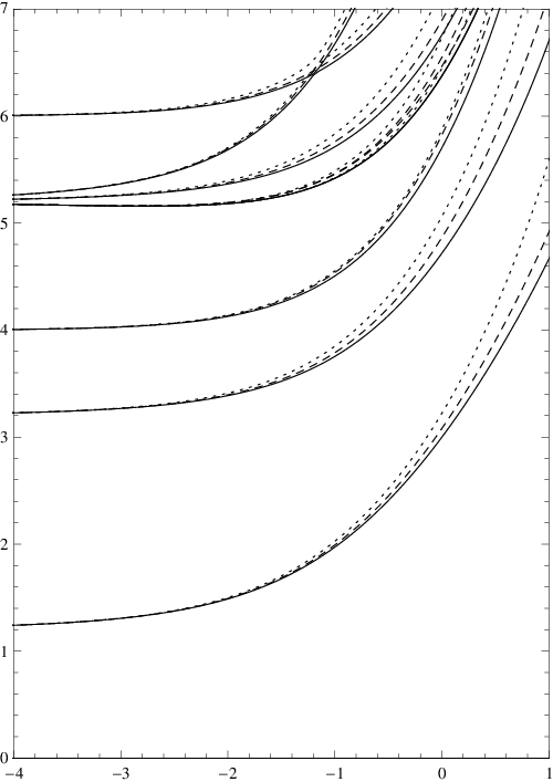
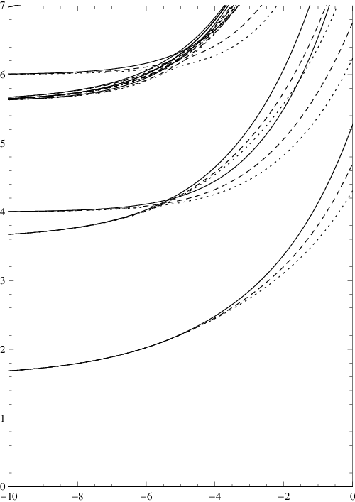
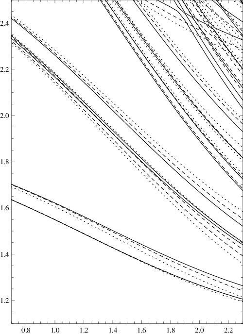
In figure 4(a), we reproduce figure 7 from [3] showing the scaling functions plotted against $r$ . The solid lines the bare TCSA data and the various dotted and dashed lines are the BY approximations to these energy levels. There is a general agreement, but we do not think it is good enough to confirm the BY energy levels as correct. As Klassen and Melzer say, the main problem is not with the BY levels but with truncation errors in the TCSA. In figure 4(b), we correct the TCSA data by the 1-loop renormalisation and rescaling formulae we have found.

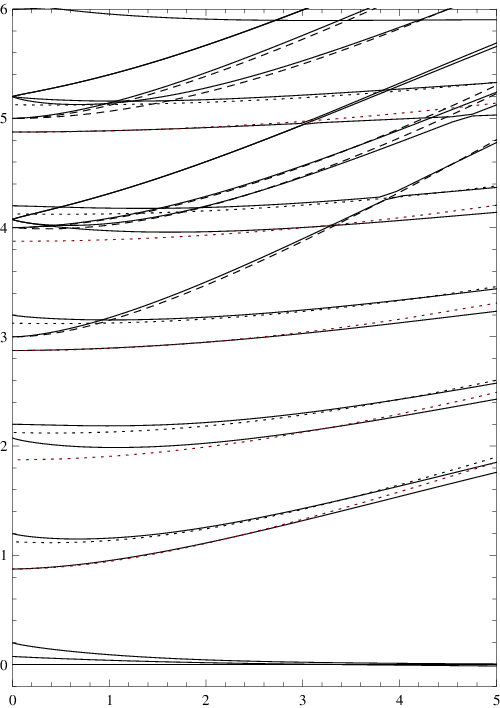
There is a dramatic increase in agreement with the BY results for the renormalised, re-scaled gaps compared to the bare gaps; they still disagree for small $r$ as is to be expected for the approximate BY solutions, but the agreement for middling ranges of $r$ , say $2<r<4$ , is excellent. In this range, the exponential corrections to the BY solutions have been suppressed and the 2-loop corrections to the renormalisation and rescaling formulae are still small. For $r>4$ the 2-loop corrections to the renormalisation and re-scalings are large enough to show a qualitative difference between the TCSA and BY gaps.

Another noticeable effect of the rescaling is to improve the behaviour of the ground states in each sector - the inclusion of the shifts $\delta_{i}$ makes a qualitative difference in the convergence of the ground states; we show these regions in figure 5 where we plot the energy gaps from the bare TCSA data and the RG improved TCSA data together with the difference of the ground states in the $(1,*)$ and $(2,*)$ sector calculated using the TBA system of [20]. There is a clear difference between the ground states at $r=5$ whereas in figure 5(b) this has been substantially decreased and the region of good agreement with the TBA extended from the region $r<0.6$ to $r<2$ .

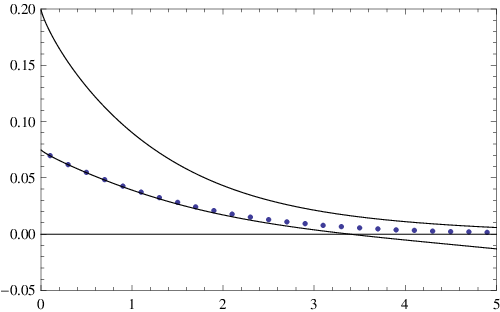
We can show that it is only the form of the renormalisation and re-scalings used in figure 4(b) that are wrong by choosing to fit the TCSA data to the BY data, and so deduce effective re-scalings and renormalisations. We choose to fit the first two gaps in the even sector to find these numerical renormalisation and re-scaling, and use these for the rest of the data. This empirically renormalised and rescaled TCSA data is shown in figure 4(c) along with the BY data, where we have chosen to remove the exponential corrections to the ground states in each sector and set them to be zero. The agreement is impressive, even for $r$ as large as 12, confirming that the TCSA data is indeed very accurate once the renormalisation and rescaling has been taken into account. To give some idea of the size, at $r=12$ the empirically calculated rescaling and renormalisation functions at level 9 are $r_{9}=0.76$ and $g_{9}=0.71$ .

We can use the empirically calculated rescaling to check the scaling form predicted from (4.18), that is

r_{n}(\lambda)=r(\lambda n^{(1-2y)/2})\;,\;\;r_{\text{1-loop}}(x)=\left(1+\frac{x^{2}}{4\Gamma(2h)^{2}(2\pi)^{2y-1}}\right)\;.

(5.4)

In figure 6, Correspondingly, we plot the estimate of and 1-loop approximation to $r(x)$ in figure 6. We see that there is actually good agreement with both the scaling form and numerical value of the function.

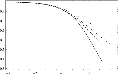
This can not be said of the renormalisation function $g_{n}(x)$ . The inaccuracy of the BY approximation for small $\lambda$ or $r$ means that we cannot effectively use it to check the form of the perturbative renormalisation function $g_{n}(x)$ . For large values of $r$ we see a definite disagreement with both the numerical value of and the scaling form of the 1-loop prediction. For large values of $r$ , we see $g_{n}(x)\sim g(xn^{-0.3})$ , the same form as the rescaling function. Since this is a larger exponent than that predicted from 1-loop, which would be $g(xn^{-0.6})$ , it is quite possible that the larger exponent is correct, arising from higher loop corrections, just as the exponent for the rescaling comes from a second order effect. The best hope we have of checking this in detail is for the exact TBA excited state spectrum to be calculated on the cylinder which would allow comparison with $g_{\text{1-loop}}$ down to small values of $r$ .

6 Divergence for $h>3/4$

One of the main predictions of equation (4.18) for the rescaling functions is the exponent of $n^{4h-3}=n^{1-2y}$ . This goes to zero for large $n$ for $h<3/4$ but diverges for $h>3/4$ , so the rescaling function will diverge with increasing $n$ for $h>3/4$ . Since this is the leading $n$ -behaviour in the scaling function gaps, it suggests strongly that the TCSA scaling function gaps will only converge to the exact answer for $h<3/4$ . This means that any application of the bulk TCSA on the cylinder for $h>3/4$ will only be able to predict the ratio of energy gaps. As a demonstration, we give here the first few scaling function gaps for $\mathcal{M}A_{4}^{(+)}$ with $h=3/5,4h-3=-3/5$ and for $\mathcal{M}A_{9}^{(+)}$ with $h=4/5,4h-3=1/5$ . As can be seen, the gaps decrease with increasing level for $\mathcal{M}A_{4}^{(+)}$ , in accordance with the prediction that the rescaling function decreases with increasing $n$ . On the other hand, the gaps increase for $\mathcal{M}A_{9}^{(+)}$ , showing no sign of convergence, in accordance with the divergence of the perturbative rescaling function.

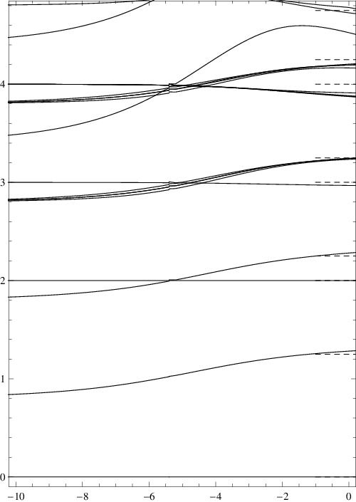
This does not mean that the TCSA contains no useful data - there is good evidence that the ratio of the energy gaps still remains physical, even if the gaps themselves diverge. In figure 7(c) we show the ratio of the energy gaps $2\tilde{e}_{i}/\tilde{e}_{3}$ for the same range as 7(b), showing that they are converging nicely to the expected $(*,1)$ sector of $M_{8,9}$ (the dashed lines on the right of that plot).

7 Complications for bulk perturbations on the strip

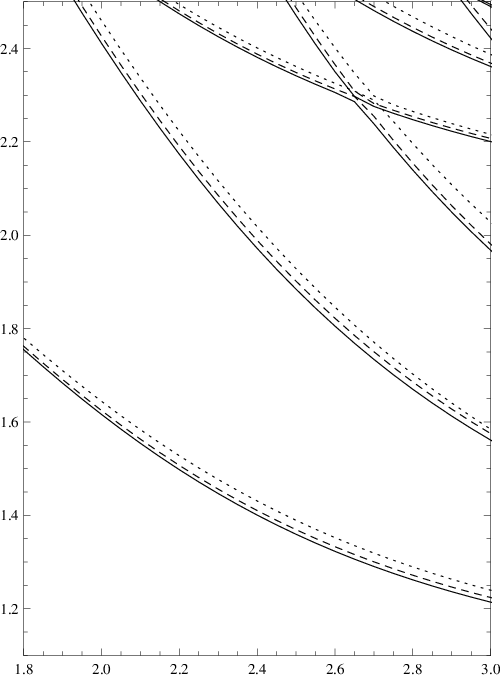
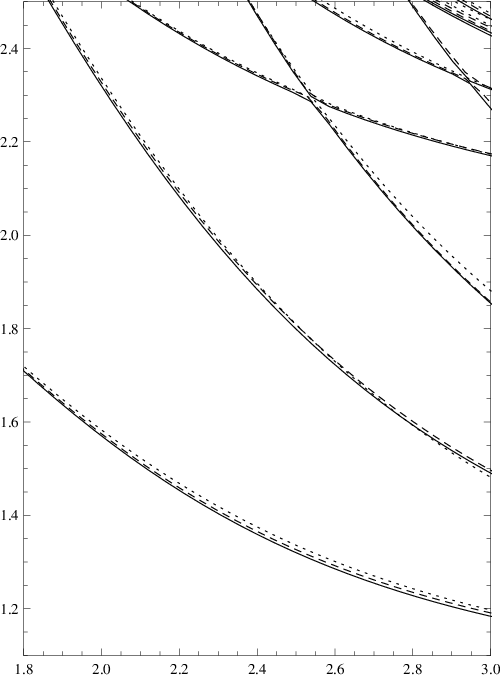
So far we have not discussed the TCSA method applied to bulk perturbations on the strip. This was first used in [11] where it proved very accurate for the Lee-Yang model (for which $y=12/5$ ). We would like to make a similar analysis to that here to find the leading truncation effects on the spectrum, but the form of the correlation functions on the strip make this much harder and so far we have not been able to find even the leading term such as a coupling constant renormalisation. There is however, numerical evidence to suggest that there are in fact no such simple renormalisation and rescaling effects on the strip. In figure 8 we show the effect of changing truncation level on the scaled energy gaps in the massive perturbation $\mathcal{M}A_{4}^{(-)}$ on the cylinder and the strip. Since we look at the ratio of energy gaps, the ground state energy and rescaling terms are removed, and we should see simply the effect of the coupling constant renormalisation. In figure 8(a) this is exactly what we see for the model on the cylinder: as the level is increased, the lines all move to the left, suggesting that a renormalisation of the coupling is required. In figure 8(b) we perform the 1-loop coupling constant renormalisation from 4.18 and indeed the TCSA data from the different levels are renormalised onto a single set of lines.

In figure 8(c), however, we show the scaled energy gaps for the same model on the strip with $(1,1)$ boundary conditions on each edge. In this case, as the truncation level is altered there is no consistent movement of the lines to the left or the right, indeed the second gap appears to be almost invariant under the change of the level. It is clear that no single coupling constant renormalisation will make the TCSA data from the various levels map into a single set of lines; the leading truncation effect on the TCSA on the strip is not a simple coupling constant renormalisation.

8 Conclusions

We believe we have presented good evidence that the leading corrections to the TCSA method on a cylinder are a possible ground-state divergence, a coupling constant renormalisation and a representation-dependent energy re-scaling. Application of these to the early tests of TCSA in [2] and [3] have greatly improved the accuracy and reliability of the TCSA method which appeared to be very poor in those cases. One by-product has been the important result that the TCSA does not actually converge for perturbations with $h>3/4$ where there is a divergent energy rescaling, but we have presented evidence that the ratio of energy gaps does still converge in this case.

We would like to point out that the perturbative renormalisation and rescaling use no more information than is usually available when using the TCSA – the scaling dimensions, three-point couplings and modular S–matrix. In this way we think of them as an improvement of the TCSA. They do not require knowledge of the four-point functions or conformal blocks which can be difficult to calculate, even for minimal models [12].

It has also been suggested [24] that the TCSA may have a finite radius of convergence for any $n$ . The apparent lack of convergence in $n$ for the first even gap of $\mathcal{M}A_{4}^{(+)}$ in figure 2(a) might be a sign of this, although since this occurs when the scaling function is greater than its IR value, it is also possible as we suggest that this divergence occurs after the IR fixed point is reached, which we expect to be at a finite value of $n$ tending to infinity as $n$ increases.

The results have found now allow one to apply the TCSA in a wide variety of cases where it was not thought useful before, in particular we hope to use it to study irrelevant perturbations in the light of the results on irrelevant boundary perturbations in [16].

9 Acknowledgements

PG would like to thanks STFC for support under studentship PPA/S/S/2005/04104 and ST/I505748/1. GMTW would like to thank G. Takács and G.Zs. Tóth for helpful discussions, G. Takács for comments on the paper and STFC grant ST/G000395/1 for support. All numerical calculations were performed using Mathematica [25].

	$\displaystyle{\langle{\varphi_{i}}\|}\varphi_{j}(w,\bar{w}){{\|{0}\rangle}}$	$\displaystyle=$	$\displaystyle\delta_{ij}\|w\|^{-2h_{i}}\;,$
	$\displaystyle{\langle{\varphi_{i}}\|}\varphi_{j}(1,1)\varphi_{k}(w,\bar{w}){{\|{0}\rangle}}$	$\displaystyle=$	$\displaystyle\frac{C_{ijk}}{\|1-w\|^{2(h_{i}-h_{j}-h_{k})}}$		(3.4)

References

- [1] V.P. Yurov and A.B. Zamolodchikov, Truncated conformal space approach to the scaling Lee-Yang model, Int. J. Mod. Phys A5 (1990) 3221–3245.
- [2] M. Lässig, G. Mussardo and J.L. Cardy, The scaling region of the tricritical Ising model in two dimensions , Nucl. Phys. B 348 (1991) 591-618.
- [3] T.R. Klassen and E. Melzer, Kinks in Finite Volume, Nucl. Phys. B382 (1992) 441-485, hep-th/9202034v1
- [4] Z. Bajnok, L. Palla, G. Takács and F. Wágner, The k-folded sine-Gordon model in finite volume, Nucl. Phys. B587 (2000) 585-618 [hep-th/0004181]
- [5] B. Pozsgay and G. Takács, Characterization of resonances using finite size effects Nucl. Phys. B748 (2006) 485-523 [hep-th/0604022]
- [6] A. Mossa and G. Mussardo, Analytic properties of the free energy: The Tricritical Ising model, J. Stat. Mech.0803:P03010, 2008 [arXiv:0710.0991]
- [7] G. Mussardo and G. Takács, Effective potentials and kink spectra in non-integrable perturbed conformal field theories, J. Phys. A42:304022, 2009 [arXiv:0901.3537]
- [8] L. Lepori, G.Zs. Toth and G. Delfino, Particle spectrum of the 3-state Potts field theory: A Numerical study, J. Stat. Mech. 0911:P11007, 2009. [arXiv:0909.2192]
- [9] R.M. Konik and Y. Adamov, A Numerical Renormalization Group for Continuum One-Dimensional Systems, Phys. Rev. Lett. 98 (2007) 147205 [arXiv:cond-mat/0701605]
- [10] G.P. Brandino, R.M. Konik and G. Mussardo, Energy level distribution of perturbed conformal field theories , J. Stat. Mech. (2010)P07013 [arXiv:1004.4844]
- [11] P. Dorey, A. Pocklington, R. Tateo and G. Watts, TBA and TCSA with boundaries and excited states, Nucl. Phys. B 525 (1998) 641 [hep-th/9712197].
- [12] P. Di Francesco, P. Mathieu and D. Sénéchal, Conformal Field Theory, Springer-Verlag New York (1997).
- [13] G. Feverati, E. Quattrini and F. Ravanini, Infrared Behaviour of Massless Integrable Flows entering the Minimal Models from , Phys Lett. B 374 (1996) 64-70, hep-th/9512104v2
- [14] G.Zs. Tóth, A study of truncation effects in boundary flows of the Ising model on a strip, J. Stat. Mech. (2007) P04005, hep-th/0612256
- [15] G. Feverati, K. Graham, P.A. Pearce, G.Zs. Tóth and G.M.T. Watts, A renormalisation group for the truncated conformal space approach, J. Stat. Mech. (2008) P03011 [hep-th/0612203]
- [16] G.M.T. Watts, On the renormalisation group for the boundary truncated conformal space approach [arXiv:1104.0225]
- [17] I. Runkel, Boundary structure constants for the A-series Virasoro minimal models, Nucl. Phys. B549 (1999) 563–578, [arXiv:hep-th/9811178]
- [18] M. Kórmos, I. Runkel and G.M.T. Watts, Defect flows in minimal models, JHEP 0911:057 [arXiv:0907.1497]
- [19] T.R. Klassen and E. Melzer, The thermodynamics of purely elastic scattering theories and conformal perturbation theory, Nucl. Phys. B350 (1991) 635–689.
- [20] T.R. Klassen and E. Melzer, Spectral flow between conformal field theories in 1+1 dimensions, Nucl. Phys. B370 (1992) 511–550.
- [21] G. Takács, private communication.
- [22] Al.B. Zamolodchikov, From tricritical Ising to critical Ising by thermodynamic Bethe ansatz, Nucl. Phys. B358 (1991) 524–546
- [23] Al.B. Zamolodchikov, Thermodynamic Bethe ansatz for RSOS scattering theories, Nucl. Phys. B358 (1991) 497–523
- [24] P.E. Dorey, private communication.
- [25] Wolfram Research Inc, Mathematica, version 8.0, Champaign Illinois, 2010.