Evolution of to the adiabatic limit
Abstract
We study inflationary perturbations in multiple-field models, for which typically evolves until all isocurvature modes decay—the “adiabatic limit”. We use numerical methods to explore the sensitivity of the local-shape bispectrum to the process by which this limit is achieved, finding an appreciable dependence on model-specific data such as the time at which slow-roll breaks down or the timescale of reheating. In models with a sum-separable potential where the isocurvature modes decay before the end of the slow-roll phase we give an analytic criterion for the asymptotic value of to be large. Other examples can be constructed using a waterfall field to terminate inflation while is transiently large, caused by descent from a ridge or convergence into a valley. We show that these two types of evolution are distinguished by the sign of the bispectrum, and give approximate expressions for the peak .
1 Introduction
In single-field inflation with canonical kinetic terms, the curvature perturbation produced at horizon crossing is conserved with nearly Gaussian statistics [1, 2]. Multiple-field models support a richer phenomenology, driven by a flow of power from isocurvature modes into the curvature perturbation. This flow is sourced dynamically, and where only canonical kinetic terms are present the dynamics are determined by the potential. Therefore, there is some hope that we may use one to learn about the other.
How much information could be extracted? A general potential is a complicated landscape, and it is unlikely that observations will be sufficient to single out a specific shape. But by piecing together clues from dynamical evolution it may be possible to obtain information about the topography of the landscape in our local neighbourhood. This is a form of potential reconstruction [3, 4, 5].
Sensitivity to dynamical effects is helpful when distinguishing observational outcomes. Unfortunately, it complicates the task of extracting predictions. In principle, the statistics of the curvature perturbation should be tracked until the time of last scattering—where the microwave background anisotropy was imprinted—and in our present state of ignorance this is an impossible undertaking. Therefore, to connect the physics of inflation with observation, we must rely on conservation: if the isocurvature modes are exhausted, quenching the flow of power into the curvature perturbation, it will cease to evolve. It is the statistics which apply at the onset of conservation which will be inherited by observable quantities.
This point of view was developed soon after multiple-field models entered the literature [6]. For practical purposes we require a characterization of the conditions under which becomes constant. In the absence of isocurvature modes, conservation of was demonstrated by Rigopoulos & Shellard [7], Lyth, Malik & Sasaki [1] and later Langlois & Vernizzi [8, 9, 10, 11, 12] using a gradient expansion. Christopherson & Malik extended these results to models in which the Lagrangian can be an arbitrary Lorentz-invariant function of the scalar field and its first derivatives [13]. More recently, Naruko & Sasaki and Gao [14, 15] applied similar arguments to higher-derivative models which preserve second-derivative field equations, where conservation can be subtle [16, 17]. Weinberg developed a different approach [18, 19, 20, 21], adapting the techniques of Goldstone’s theorem to show that would become massless on superhorizon scales, admitting a time-independent solution. Whether this solution is selected is a model-dependent question.
The statistics of are fossilized in the radiation fluid at last scattering, and its two-point correlations have been studied since their presence was confirmed by cobe [22, 23]. More recently, sophisticated Cosmic Microwave Background (cmb) experiments have raised the possibility that three- and higher -point correlations may be detectable [24, 25]. These correlations are interesting because, in principle, they are sensitive probes of physical processes and dynamical conditions in the early universe [2, 26, 27, 28, 29]. But precisely because of these desirable properties, such observables carry an unavoidable risk: they may be equally sensitive to subsequent dynamics, including the process by which becomes conserved. We may learn important physics from studying the details of this process—but it need have little to do with our theories of the very early universe, and if we wish to use -point correlations to study these theories then we should proceed with caution. For this reason it is important to understand which predictions of early-universe models can be connected reliably to late-time observations.
Our imprecise knowledge of physics above the TeV frontier means it is not possible to give a complete answer. In this paper we pursue a more modest objective. Focusing on three-point correlations—with amplitude measured by [24]—and considering models where the flow of power from isocurvature modes is quenched at or near the end of inflation, we study how the asymptotic value of depends on the process by which the isocurvature modes become exhausted. We refer to this exhausted state as the adiabatic limit. Our arguments are phrased in terms of three-point correlations, but many of our conclusions are general and apply to arbitrary -point functions including the two-point function.
Classification of models.
We restrict attention to models where a significant is generated dynamically by inflation. This excludes examples such as the curvaton [30, 31] or modulated reheating [32, 33] which rely on an inflationary seed perturbation but amplify it by a noninflationary mechanism. If we disallow noncanonical kinetic terms, Maldacena’s result guarantees that the models of interest must include two or more dynamically relevant fields [2].
Under these conditions, field fluctuations are generated at horizon crossing with almost Gaussian statistics [34, 35, 36]. However, unlike single-field inflation, these perturbations may cause spatially separated regions of the universe to experience different expansion histories. The set of phase space trajectories associated with an ensemble of such regions is initially a narrowly collimated bundle whose ‘width’ is set by quantum scatter. (We give details in §2.) The curvature perturbation is a precise measure of the relative expansion between spatial patches. Therefore its evolution is a consequence of focusing or defocusing of the bundle: as nearby patches of the universe evolve towards or away from each other in phase space, they experience varying expansion rates. In the adiabatic limit, the bundle degenerates to a caustic. Its width shrinks to zero, and all trajectories converge to a single line.
When does convergence occur? The answer is model-dependent, but we can recognize broad classes of behaviour.
- •
The potential may contain a focusing region, which enables trajectories to converge ‘naturally.’ If inflation ends in the vicinity of this region, an adiabatic limit is automatic. Examples include Nflation and related models [37, 38, 39, 40, 41, 42, 43]. However, one is always free to build models in which the adiabatic limit is achieved differently, perhaps by a waterfall transition. If the ‘natural’ limit is employed, there are two relevant questions.
First, is the limit achieved before the end of inflation? If so, it is not necessary to specify details of the subsequent phases. Otherwise, we must choose among the various scenarios for reheating and later dynamics, and the predictions of the model may depend on our choice.
Second, in the case where an adiabatic limit is reached during inflation, does this occur before the slow-roll approximation fails? This raises no issues of principle, but may influence how one chooses to study the model; for example, numerical methods may be required. We will return to this question in §5.
- •
Alternatively, there may be no natural means by which trajectories converge. In such models there is no alternative: the inflationary model does not make unambiguous predictions by itself, but only when embedded in a larger scenario which determines at least the mechanism by which inflation ends and the universe reheats.
None of these observations are new, but their application to non-Gaussian statistics has yet to be studied in detail.
Accepting the separate universe principle, to be discussed in §2 below, one obtains explicit expressions for the -point functions of the curvature perturbation [28] which automatically respect these conclusions. Therefore, concrete predictions can be obtained whenever it is possible to calculate these expressions accurately until the onset of conservation. However, in many cases this ideal procedure is impossible or impractical. Working in a special class of models where the potential is separable, Meyers & Sivanandam [44, 45] argued that the connected -point correlation functions would be damped towards slow-roll suppressed values. Our analysis is closely related, but we argue that the value achieved in the adiabatic limit need not be especially small [43]. Indeed, in some cases, the adiabatic limit is associated with growth towards the asymptotic value, rather than decay.
Objectives.
In this paper we apply these ideas to the primordial bispectrum, and its amplitude in the squeezed limit. There are three principal objectives. First, we illustrate that local can be sensitive to details of when and how the adiabatic limit is reached. Using examples, we demonstrate that—even in models where convergence occurs naturally— may depend on the details of this process. Second, the calculations necessary to obtain a precise estimate of can be technical, perhaps requiring recourse to numerical methods. For some models, simple techniques exist which allow a qualitative estimate of the evolution and asymptotic value of . We outline these methods and apply them to simple examples. Third, we use numerical methods to perform a detailed study of the evolution of in a selection of models. By themselves these calculations already reveal interesting patterns of behaviour, but also provide guidance regarding the asymptotics of models where an adiabatic limit is reached only through the intervention of post-inflationary dynamics.
Outline.
The plan of the paper is as follows. In §2 we discuss the separate universe approach to perturbation theory in phase space, and the formalism. In §3 we discuss mechanisms for generating large evolving local non-Gaussianity, and estimates for the maximum value and its dependence on initial conditions. §4 includes a brief account of analytic expressions for estimating , and discusses conditions necessary for this value to be large. §5 reports a detailed numerical study of in a selection of models with two or more fields. We conclude in §6. An Appendix contains details of some analytic calculations.
2 Phase space description of slow-roll inflation
Consider inflation driven by multiple canonical scalar fields (where ), self-interacting through a potential . Defining , the scalar equations of motion are
| (2.1) |
Inflation occurs when . Eq. (2.1) generates a -dimensional phase space . In the “slow-roll” limit where there is a dynamical attractor, allowing the decaying mode to be discarded and restricting evolution to an -dimensional submanifold on which (for example) the are determined in terms of the . The growing mode on satisfies . In the slow-roll limit it is possible to write as a sum of independent contributions from each field, yielding , where the satisfy
| (2.2) |
In simple models it may happen that the matrix also has small components .
Density fluctuations are generated by the inflationary background and can be measured by the curvature perturbation on uniform density spatial hypersurfaces, denoted . For cosmological purposes its statistical properties are characterized by low-order correlation functions, of which the first two are
| (2.3a) | ||||
| (2.3b) | ||||
The amplitude of the three-point function is usually measured in terms of a momentum-dependent parameter , satisfying
| (2.4) |
where , . The problem at hand is to calculate .
Bundles of trajectories.
A comoving scale is outside the horizon when , where is the scale factor and is the Hubble parameter. An overdot denotes a derivative with respect to time. During inflation is approximately constant, whereas is growing rapidly. Therefore rapidly becomes negligible a few e-folds after horizon crossing. Smoothing over a comoving scale somewhat larger than , widely separated spatial patches will locally evolve like an unperturbed universe up to small corrections. This is the separate universe picture [46, 47, 48].
An ensemble of smoothed regions picks out a collection of trajectories in phase space. If the ensemble is drawn from a spacetime region of finite comoving extent then we can expect this collection to be narrowly collimated provided is not too large.11 1 Comoving quantities such as are not physical, and can not appear in predictions for observable quantities [49]. The discussion in this paper is independent of , but as a point of principle should be removed from physical quantities by supplying a distribution function for the large-scale modes [50, 51, 52]. After doing so, all predictions depend only on physical scales. Similar conclusions have been obtained by a number of different methods [53, 54]. We refer to this ensemble of clustered trajectories as a bundle. When making predictions for microwave background scales it may contain of order trajectories or more [55]. In practice the analysis is simplified by working in a thermodynamic limit where the bundle formally contains an infinite number of trajectories. To avoid spurious infrared problems we should demand that these reheat almost surely in the same vacuum.
The isocurvature modes label Fermi normal coordinates on , adapted to the bundle. Each isocurvature field has equation of motion and constitutes a conserved quantity [56, 6]. Together, these conserved quantities identify a trajectory. A particular location on each trajectory is specified by the integrated expansion . This ‘trajectory’ approach can be traced to Hawking’s formulation of perturbation theory [57], and was applied to inflation by several authors [46, 58, 59, 60]. An explicit description in terms of trajectories on was given by Salopek [56] and García-Bellido & Wands [6]. Locally, and the isocurvature fields generate a coordinate chart on . Fluctuations along the same trajectory generate the adiabatic mode, . Isocurvature modes represent fluctuations between trajectories. In an -field model, the reduced phase space supports isocurvature modes.
Bundle sections.
Consider a foliation of by submanifolds which are nowhere tangent to the bundle. An important example is foliation by surfaces of fixed energy density. We may use any such foliation to replace as a label for length along the trajectories. Intersecting the bundle with an individual hypersurface generates a cross-section with coordinates inherited from the isocurvature modes. For example, working on uniform density hypersurfaces, the scalar fields take values . These “coordinates” are not independent but are subject to the constraint , leaving the expected isocurvature labels.
If the bundle has degenerated to a caustic then each hypersurface intersects the bundle at a unique point . Making a small change of trajectory earlier in the bundle’s evolution, one will observe no change in . Therefore and we conclude . One can regard this as a requirement that physical predictions computed from statistical properties of the bundle become independent of its initial conditions. Speaking loosely, we describe this behaviour as an “attractor.” The attracting trajectory is the caustic, and we will sometimes refer to it as the limiting trajectory. An ensemble of smoothed patches traversing the limiting trajectory differ only by their relative position within it, making conserved.
This argument identifies regions where with regions where is conserved.22 2 The condition that is sufficient to show that that becomes conserved within the separate universe picture, but this argument does not demonstrate that it is necessary. We describe it as the adiabatic limit. In what follows we will see that estimates of the decay rate of play an important role in analysing the adiabatic limit. As an example, consider the purely scalar dynamics associated with slow-roll inflation. A common type of limiting trajectory lies on a valley floor in the landscape generated by the potential. Descending into the valley, the mass-squared matrix associated with perturbations orthogonal to the direction of motion should be nondegenerate, with all eigenvalues large and positive. Taking the smallest eigenvalue of magnitude one will generically find . We will discuss this example more carefully in §4.
Bundle averages.
These principles give a procedure to determine the statistics of in an adiabatic limit. One uses the bundle of trajectories to determine any required -point correlation functions, and then imposes the requirement . Unfortunately there is no unique way to do so. Different approaches to the limit correspond to different focusing mechanisms. As we have explained, focusing regions may occur naturally in some models; the examples studied by Meyers & Sivanandam [44, 45] are of this type. But whether or not a model naturally contains an adiabatic limit we may usually elect to impose a different one, perhaps by enlarging the field content to include a waterfall transition. We will study some possibilities below.
It is first necessary to obtain the relevant correlation functions. When the slow-roll attractor is operative, the e-foldings along each trajectory can be expressed as a function of its initial conditions. Therefore . Expanding in the neighbourhood of a fiducial trajectory yields
| (2.5) |
where and . The measure deviations from the fiducial trajectory, and will typically be of order the quantum scatter. After restriction to connected correlation functions there is no dependence on the arbitrary choice of fiducial trajectory.
Eq. (2.5) enables the low-order correlation functions to be expressed in terms of the data , , which can be computed in some models [39, 61, 44]. One finds , which determines the power spectrum (2.3a). Similarly, can be written33 3 We are neglecting intrinsic non-Gaussianities of the . For slow-roll inflation with canonical kinetic terms these are negligible whenever is large enough to be observable [62, 39]. [28]
| (2.6) |
3 Transitory behaviour of
It was explained in §§1–2 that our interest lies in adiabatic regions where all isocurvature modes are exhausted, preventing further evolution of . This limit need not be achieved smoothly. For example, in hybrid scenarios the inflationary phase is suddenly destabilized by a waterfall transition, leading to abrupt convergence of trajectories. Although a convincing demonstration has not yet been given, in some circumstances the subsequent dynamics may preserve the value of at the waterfall. This strategy has been invoked by various authors [63, 64, 65, 66]. Some fine-tuning would be required to arrange at the transition point. Nevertheless, in these scenarios and others it may be misleading to focus exclusively on regions where phase space trajectories naturally converge. For this reason we pause to study the qualitative evolution of , whether or not we are close to an adiabatic region. We focus on scenarios where its value changes rapidly, before returning to focusing regions in §4.
Under which circumstances should we expect the moments of the distribution function to change significantly? The distribution function describes how trajectories cluster around the core of the bundle. It is conserved under linear evolution, but is sheared or distorted on curved paths [67, 68]. These effects reshape the distribution function: even when it is initially Gaussian we expect probability to be relocated from the core to the outer layers of the bundle. This is associated with the generation of significant third- or higher -order moments.
Curved paths can be generated by many choices of microphysics. We study only an especially simple mechanism. Where the potential’s topography includes a ridge or valley we will encounter curved trajectories diverging from the ridge or converging into the valley floor. Examples of such trajectories have been studied by a number of authors [40, 65, 66, 69].
3.1 Ridges: Diverging trajectories
We restrict attention to two-field models, which already capture the principal dynamical features, and label by coordinates and . We assume a “ridge” or separatrix at . In the neighbourhood of an arbitrary point on the ridge the potential will generically have the form . The mass-squared is positive, and omitted terms are higher-order in and . These become relevant at some point after the trajectory has been ejected from the vicinity of . The trajectory is classically stable, although depopulated by quantum fluctuations [70, 71, 72, 73, 74].
Trajectories.
Measuring length along each trajectory by the energy density, the evolution equations are
| (3.1a) | ||||
| (3.1b) | ||||
According to (3.1b), a trajectory emanating from and evolving to satisfies
| (3.2) |
If then the logarithm dominates and the trajectories disperse linearly in the sense , where the growth factor satisfies and . Nonlinear dispersion occurs in the region where the quadratic term dominates. The transition between the two is the “turn,” beyond which each trajectory is ejected from the ridge and rapidly evolves to . At the turn we have
| (3.3) |
which makes the kinetic energy in each field roughly equal, .
This leads to the following physical picture. Trajectories which are still close to the ridge preserve their initial Gaussian profile. Trajectories populating the downhill-edge of the bundle quickly slide away, generating a heavy tail at large . In this region kinetic energy has greater relative importance, slowing the expansion rate and enhancing the frequency of excursions to large negative . Therefore this mechanism will generate negative from a Gaussian distribution.
Whether a large negative amplitude is achieved in practice depends on the initial distribution of trajectories within the bundle, the nonlinear relation between the fields and , and for how long the mechanism operates. Sufficiently far down the ridge the trajectories depend on the completion of . Therefore, the approach to an adiabatic limit cannot be described by the techniques of this section.
analysis.
We now translate to and repeat the analysis in the language of the method [28]. Consider two trajectories originating well before the critical turning point, but initially separated by a distance . It is useful to define , where indicates the initial point is very close to the ridge. In this region surfaces of constant energy density in practically coincide with surfaces of constant . Therefore, to bring this pair of trajectories to a common energy density requires a small excess expansion . The subsequent expansion history, measured to a surface , can be written .
In what follows we work without loss of generality on the positive branch , and suppose and remain sufficiently small that higher-order terms in the potential do not become relevant. Once this assumption fails, may acquire a nonnegligible dependence on , potentially invalidating our conclusions. Passing to the limit where and become infinitesimal, we conclude that on arrival at the trajectories have experienced expansion histories which differ by
| (3.4) |
where the partial derivative is to be evaluated at constant and .
Invoking the chain rule, Eq. (3.4) determines all derivatives of . We find
| (3.5) |
So far our considerations have been general. Prior to the turn, Eq. (3.2) makes negligible whereas is exponentially growing. In this region our assumptions make the integrands of Eqs. (3.4) and (3.5) positive, and therefore both and are negative and decreasing.
If is not too small, the integrals of (3.4) and (3.5) are dominated by their upper limits—where the exponential growth is maximized. Taking the initial evolution in to be almost negligible, this requires
| (3.6) |
where the approximate equality applies if is at least a little smaller than . If is to be sufficiently light to acquire a quantum fluctuation then , and if both conditions are to be compatible we must require . A short calculation yields
| (3.7a) | ||||
| (3.7b) | ||||
This relation between and is a consequence of the exponential growth of prior to the turn.
Initially, and are small in comparison with and . In addition, is constant and can safely be neglected. Therefore is dominated by the fluctuation in , which is practically Gaussian. Using (2.6), we find
| (3.8) |
While , the first term dominates and (3.8) gives . As the trajectory moves away from the ridge the -derivatives become increasingly important whereas the -derivatives are constant. When and are comparable, is dominated by the second term in (3.8). In virtue of (3.6) and the initial condition , this is much larger than and causes a spike in . Estimating the peak to occur when , we find
| (3.9) |
where is the standard -parameter associated with . In this expression and similar ones below, including Eq. (3.18), the numerical prefactor is uncertain by an quantity which depends on the precise balance between and at the peak.
On approach to the spike, Eq. (3.8) predicts that is negative and growing like . Subsequently, continues to increase and eventually dominates . In this region is composed almost entirely of the fluctuation. The non-Gaussianity becomes practically independent of and decays like . These estimates of the growth rate and decay rate are valid before the turn, where is growing exponentially as described below Eq. (3.2).
Dropping numerical factors of order unity and using (3.3) to estimate when the fiducial trajectory passes the turn, we find
| (3.10) |
This is much less than Eq. (3.9) and therefore occurs some time after the peak is achieved. If Eq. (3.10) is not invalidated by higher-order terms in the potential, it implies that the height of the spike is adjustable independently of on entry or exit. Since the peak occurs before most trajectories in the bundle reach the turning point (3.3), our analysis will apply provided these higher-order terms become relevant only after the turn.
Scaling relations.
Eqs. (3.8) and (3.9) give interesting scaling relations for the peak , and for its growth and decay near the spike. Eq. (3.9) suggests that the maximum attained during the spike has a practically universal power-law scaling for any potential which can be approximated by the coefficients and up to the turn of the trajectories: for such potentials we should expect with exponent . In §5 we will use numerical methods to study models which exhibit this scaling behaviour.
3.2 Valleys: Converging trajectories
The converse process occurs when a trajectory approaches a valley, where a bundle of trajectories is nonlinearly focused rather than defocused. As above, we specialize to a two-dimensional field space labelled by coordinates and suppose there exists a valley aligned with the direction. In the neighbourhood of the valley we write , where is a constant and
| (3.11a) | ||||
| (3.11b) | ||||
If then the slopes will be relatively steep in comparison with the valley floor. Omitted terms are higher order in and , but become increasingly irrelevant as , . Sufficiently far from the motion is almost entirely in the direction.
During descent into the valley, trajectories populating the uphill edge of the bundle experience a larger velocity in the orthogonal direction compared to those lower down the slope. Therefore the uphill edge is compressed towards the centroid, generating a nonlinear distribution. The tail of the distribution is again on the downhill side, but in this case the tail has lower kinetic energy and enhances the frequency of excursions to a large positive . Therefore this mechanism generates a positive .
analysis.
The evolution equations are
| (3.12a) | ||||
| (3.12b) | ||||
In analogy with the ridge case, it is helpful to define a dimensionless measure of distance, , from the valley floor. We choose , which measures the relative partition of kinetic energy between the fields. Our analysis applies when the trajectories begin from an initial position sufficiently high above the valley, where and only the -field is in motion. In this regime, Eqs. (3.12a)–(3.12b) can be integrated to find
| (3.13a) | ||||
| (3.13b) | ||||
up to corrections of relative magnitude . Eqs. (3.13a)–(3.13b) cease to be a good approximation no later than , when and the kinetic energy in each field is approximately equal. In typical models this occurs at the turn.
For , surfaces of constant energy density are practically aligned with surfaces of constant . Adopting the methods of §3.1, we bring a pair of nearby trajectories separated by the displacement to a common value of , and write the number of e-foldings to a subsequent surface of constant energy density as . Passing to the limit of infinitesimal and , and using Eqs. (3.13a)–(3.13b), we conclude that on arrival at , the trajectories have experienced expansion histories which differ by
| (3.14) |
where is to be understood as a function of and we have introduced the mass ratio . Corrections to Eq. (3.14) are suppressed by .
Eq. (3.14) reproduces many features of the ridge analysis. The derivative is constant, whereas is initially zero but growing. Performing the integral, we find
| (3.15) |
where the “growth factor” satisfies
| (3.16) |
We have assumed dominates , but the generalization to other cases is straightforward. At we have . For the dominant growing term depends on microphysical details of the model. Under our assumption the dominant growth is initially from . Inflation will not end naturally in a model of this type, so some other exit mechanism must be invoked. We will see examples of this kind in §5. On the other hand, if the logarithm will initially dominate. In either case, the asymptotic growth in the limit is from . Therefore, for a typical model is a complicated function determined by a competition for dominance between the various terms. However, remarkably, in many cases the behaviour of is almost independent of these complicated microscopic details.
Differentiating (3.15), we find
| (3.17) |
where . Eq. (3.16) implies that is growing as decreases to zero. While is increasing towards we find increases, achieving a maximum value when . First, suppose the -dependent term is subdominant at this time, which implies . We find
| (3.18) |
which is independent of the growth rate (3.16) and the mass ratio . In this sense, the maximum value (3.18) is a “universal” phenomenon. When we find that decays like , at least until , when it may stabilize as we will explain below. In analogy with the ridge, this sequence of growth and decay gives rise to a spike in . Ultimately will decrease until , and the subsequent behaviour of must be determined by different methods, such as those described in §4. Written in terms of the dimensionless measure , Eq. (3.18) coincides with (3.9) with the identification . In this language, the sign of is inherited from the sign of .
Second, consider the “nonuniversal” case where the -dependent term dominates (3.17). In this case, increases until , achieving a value larger than (3.18). Its precise value is set by the ratio , and may depend on details of the potential, including the mass ratio. When the time dependence of is set by . Its precise scaling depends on the dominant term in . In particular, if then is approximately constant and does not decay. In such cases, exhibits a plateau and it may no longer make sense to speak of a spike at all. After the turn is completed, the nonlinear deformation of the bundle will partially relax, leading to decay of . The precise details, including the decay rate, are model-dependent. Eventually the fields reach equipartition of kinetic energy and this analysis breaks down.
4 Asymptotic behaviour of
Whether a large can be generated during an epoch of slow-roll inflation—perhaps from the “spike” mechanisms described above—is irrelevant unless it can be preserved in some adiabatic limit. The methods of §3 are insufficient to resolve this question.
The potential may be such that a focusing region is naturally available. If inflation terminates in this region then the transitory evolution of studied in §3 has no necessary connection with its final asymptotic value. In certain circumstances, where the focusing region can be analysed in detail, a relatively simple statement is possible. These are the scenarios studied by Meyers & Sivanandam [44, 45]. One might have thought that the final would depend only on the local shape of the potential in the focusing region, which will typically be a stable parabolic minimum. If so, the asymptotic value of would be universal among all potentials sharing a similarly-shaped minimum. However, this is not the case. As we will explain, the asymptotic value of generally depends on properties of the potential far from the focusing region.
If multiple focusing regions are available, one must be selected by a combination of dynamics and initial conditions. To determine which possibility should be expected by late-time observers who map the anisotropy of the cmb requires an understanding of the infrared structure of the entire inflating volume [50]. This difficult “measure problem” remains unsolved.
If a natural focusing region is not available, or is not selected, then one must be imposed and the entire analysis becomes significantly more complicated. In this case the transitory evolution studied in §3 may become relevant. We will have little to say about this possibility, although we investigate some numerical cases in §5.
Natural focusing.
In this section, we study models where inflation ends in a region of the potential where the trajectories are naturally focused. Broadly speaking, two possibilities exist.
- •
The asymptotic value of generated during focusing may be unobservably small, erasing any transiently large non-Gaussianity generated by spikes or other features. This possibility was emphasized by Meyers & Sivanandam [44, 45], who worked with a particular class of separable -field models to be discussed below. However, other possibilities exist.
- •
It may be possible to make the focusing process itself generate a large by suitable choice of . An example of such a model was given by Kim et al. [43]. (Indeed, in this model, grows sharply during approach to the adiabatic limit.)
In principle, the behaviour of in a focusing region could be determined from (2.5)–(2.6) by imposing the limit . Unfortunately, it is not known how to compute the “ coefficients” and for an arbitrary model. Therefore a systematic discussion of this limit must apparently await future analytic developments.
Explicit expressions for the cofficients are known only in very restricted circumstances. Formulae for quadratic potentials were discussed by Lyth & Rodríguez [28], Lyth & Alabidi [38] and Alabidi [40]. Later, Vernizzi & Wands [39] and Battefeld & Easther [75] gave expressions for an arbitrary sum-separable potential. Taking , one finds
| (4.1) |
where satisfies
| (4.2) |
A similar expression for a product-separable potential was obtained by Choi et al. [76]. Comparable results for a general class of sum- and product-type potentials were given by Wang [61] and are summarized in the Appendix. It is also possible to take the Hubble rate to be separable rather than the potential [77, 78].
Focusing in a valley.
A typical example of a focusing region is a valley of the potential landscape, perhaps terminating in a local minimum. For fields, there are at least heavy directions with masses greater than the Hubble rate. Quantum fluctuations are suppressed in these directions, which prevent the bundle from diffusing up the sides of the valley. The steep slopes cause exponential convergence, and rapidly focus the bundle to a line.
In the neighbourhood of the valley floor, we assume it is possible to choose coordinates on field space for which the potential approximately separates
| (4.3) |
where labels distance along the valley floor—which may be a light direction—and the fields are stabilized with masses . By a suitable choice of coordinates we can arrange that . To describe a complicated valley it may be necessary to glue several such regions together. Focusing on the particular region described by (4.3), we denote the field values on entry to its domain of validity and . These will be functions of the initial fields . This initial point could generically occur far from the valley, where (4.3) need not be a good approximation.
The heavy fields evolve according to . After e-foldings from the point of entry, one finds
| (4.4) |
The total number of e-folds available within the valley is model-dependent. In a long valley the focusing may practically go to completion, making effectively zero. Alternatively, if the valley rapidly terminates in a local minimum there may be insufficient time to focus the bundle completely.
The fields can be written as linear combinations of and the , giving . The and are constants, which depend only on the choice of separable coordinates used in (4.3). They are independent of the entry point , which implies
| (4.5) |
Therefore behaves like a linear combination of derivatives .
The number of e-foldings, , which occur between the entry point and the surface will usually depend on the initial point . Assuming does not exhibit a dramatic sensitivity to these initial conditions, Eq. (4.4) shows that will decay exponentially as the trajectory settles into the valley. Potentials may exist which violate this condition, but we believe it will be satisfied for a majority of trajectories which flow over reasonably smooth potential landscapes. Where it is satisfied, this estimate of the decay rate applies once a trajectory has been captured by the focusing region, no matter what form the potential takes globally.
In Eq. (4.5) the term will typically decay exponentially, because whereas decays less rapidly. Therefore Eq. (4.4) implies the derivatives decay at least as fast as the lightest isocurvature field. We conclude44 4 The asymptotic notation indicates that and share a common decay rate.
| (4.6) |
where and is the same quantity occuring in Eq. (4.4). The final equality applies if is approximately constant during the focusing process.
Separable potentials.
In a globally sum-separable model, for which satisfies (4.1), it may happen that (4.6) is sufficiently powerful to make the final “-term” irrelevant. In these circumstances the correlation functions of , including the spectrum and bispectrum, can be determined from the remaining term of (4.1), which depends only on boundary data at the initial time. For correlation functions among fields carrying comparable momenta of order this is often taken to be the horizon-crossing time , where is the conformal time. For this reason, the scheme has sometimes been called the horizon-crossing approximation [41, 42, 43]. Despite the name, we caution that this approximation does not consist of assuming that the perturbations are constant after horizon-crossing, but rather that their values in the adiabatic limit can be determined in terms of the shape of the potential there. A similar procedure can be applied in product-separable cases.
It is less straightforward to estimate the minimum number of e-folds required to make the -terms of (4.1) negligible. Although Eq. (4.6) gives information concerning the decay rate, the number of e-folds required to damp any contribution from the -terms depends on their amplitude on entry to the valley. This is a function of each species’ relative contribution to the energy density of the universe on the initial and final slices and , from which it does not appear straightforward to draw general conclusions. However, since the isocurvature masses should be comfortably heavier than the Hubble scale, the parameter will typically be much larger than unity. In these circumstances, rather less than e-foldings are usually required to accumulate a very substantial suppression of the -terms.
In the language of Meyers & Sivanandam [44, 45], this damping of the -terms is precisely the exponential suppression which they suggested would drive the bi- and trispectrum to slow-roll suppressed values. In the language of §2 it represents focusing of the bundle to a caustic. Our analyses are entirely consistent, but it is helpful to recall that the -term in (4.1) need not be especially small. We briefly comment on this possibility at the end of this section. If that is the case, suppression of the -terms can cause the correlation functions to experience a short phase of exponential growth as they approach their asymptotic values. Note that all these conclusions depend on the existence of a globally separable potential. We are not aware of a systematic study of the asymptotics of in more general cases.
One might harbour some reservations that the -terms do not decay if the fields settle into a stable minimum, for which diverges. Near an arbitrary point, which can be chosen as the origin without loss of generality, can be written and approaches a constant. Near a minimum, one finds instead . Therefore
| (4.7) |
If the prefactor decays. Since the potential is sum-separable, we may always redefine all but one to satisfy this condition. However, if the potential is not zero at the minimum then the remaining must have nonzero . Eq. (4.7) shows that we should choose the field to have nonzero overlap with the direction of the valley floor, ie., . Under these circumstances the right-hand side of (4.7) still decays (although perhaps at a reduced rate), because by assumption decays strictly more slowly than any isocurvature mode.
Large non-Gaussianity after natural focusing.
Is it possible to obtain large at the adiabatic limit? Working in a sum-separable potential, the foregoing discussion implies that the -dependent terms in (4.1) may be discarded provided enough focusing can be achieved before the end of inflation. In general, the conditions required to achieve large may still be complicated. However, a relatively simple picture emerges if we assume that is large for one field (or at most a few such fields) [43]. Therefore, at horizon crossing dominates the analogous terms for all other fields and can be written
| (4.8) |
In a single-field model the quantity would be the inflationary -parameter. But in an assisted inflation the total potential may be much larger than [79, 80]. Therefore can remain small, making light at horizon crossing and causing it to acquire a quantum fluctuation by the usual mechanism, while can be appreciable. We study an example of this type in §5.1.2. In such models the sign of is inherited from an “enhanced” -parameter, as in Eqs. (3.9) and (3.18), but unlike these cases the enhancement is measured by the initial share of the energy density contributed by , rather than the parameters , . In Eq. (4.8) this enhancement factor is .
If several fields have comparable , their perturbations contribute equally to at the adiabatic limit and dilute any non-Gaussianity by the same interference effect which leads to the central limit theorem. Therefore the largest values of will be achieved where a single field has a dominant .
A similar discussion can be given for product-separable potentials. In this case the formulas depend solely on one field, labeled , which must be the field still evolving at the adiabatic limit. Therefore , and a large would require a violation of slow-roll. We conclude that large is not possible at the natural adiabatic limit in this class of models.
5 Models
The results of §4 show that, even for models where an adiabatic limit can be approached analytically, numerical calculations may be necessary to determine the degree of focusing which occurs near the end of inflation. In other cases there is simply no alternative.
In this section, we report the results of numerical simulations and compare the outcome to the analytic theory developed in §§3–4. In appropriate circumstances we show that the simplified description of “spikes” obtained in §3 is an accurate match for full numerical simulations. We give examples where the focusing described in §4 goes to completion—making the “horizon crossing approximation” highly accurate—and others where it does not. A case of special interest occurs when the bundle would focus only slightly after the end of inflation. One might expect that the error in analytic predictions based on the strict adiabatic limit would be small, but it transpires that can be rather sensitive to the details of the model. In models where there is no natural adiabatic region, reheating must occur before an adiabatic limit is reached. In these cases we perform a qualitative study of the dependence of on the details of the reheating phase.
Evolution after slow-roll using .
The phase space description of inflationary trajectories was discussed in §2. During multiple-field slow-roll inflation, each trajectory lies on a submanifold of the full phase space.
In a model more general than multiple-field slow-roll inflation, extra coordinates will typically be required. First, if the slow-roll approximation fails then one must work on the full phase space rather than the attractive submanifold . Therefore new isocurvature modes are typically required to label the conjugate momenta . Second, matter species other than scalar fields may be included, perhaps to describe a phase of reheating. In such cases, the full phase space splits into a Cartesian product constructed from the phase space for each species, and suitable isocurvature modes labelling all these coordinates will be required. For thermalized radiation, a common choice is the temperature, .
Several numerical approaches exist to compute the statistics of the density fluctuation [67, 68, 69]. Here we take the simple approach of calculating the derivatives of using a finite difference scheme. This requires the slow-roll approximation at horizon crossing, where initial conditions are set, but not subsequently. We have verified that our results are insensitive to changes in the step size of the finite difference scheme. Although slower than other approaches [67, 68], direct has the advantage of straightforward comparison with our analytic methods. Moreover, it requires only the evolution of an unperturbed universe, making a simple description of reheating—assuming thermal equilibrium and a single radiation fluid—easy to implement. These assumptions are at best quasi-realistic, but serve to indicate a plausible phenomenology.
5.1 Two-field models
5.1.1 Transitory models with interruption
All two-field models documented in the literature which produce large, transient exploit the spikes described in §3 [40, 65, 66]. Eqs. (3.8) and (3.9) show that to obtain large from a ridge, one must tune the initial conditions so that . Also, if this large is to be preserved in the adiabatic limit, Eq. (3.10) implies that some mechanism must operate to end inflation before the majority of trajectories in the bundle encounter the turn. In two-field models with separable potentials, the parameter combinations required to ensure these conditions were given by Byrnes et al. [65]. The observables predicted in such models depend strongly on the choice of exit mechanism. In certain cases, such as two-field hybrid inflation, it is possible that is not erased. In other cases this outcome appears unlikely.
Two-field hybrid inflation.
This model was studied by Alabidi & Lyth [40] and later by Byrnes et al. [65, 66]. The potential is
| (5.1) |
where and are slowly-rolling fields, and is a waterfall field which becomes destabilized when . We take the masses and to be positive, and assume . This ensures that the waterfall occurs at fixed energy density, making it unnecessary to account for the effect of inflation ending on different hypersurfaces [81, 63, 64, 82]. If the masses are not equal, there is a steep slope in the direction of the more massive field. The trajectories evolve along this steep direction and then turn towards the global minimum. We expect some non-Gaussianity to be generated during this process.
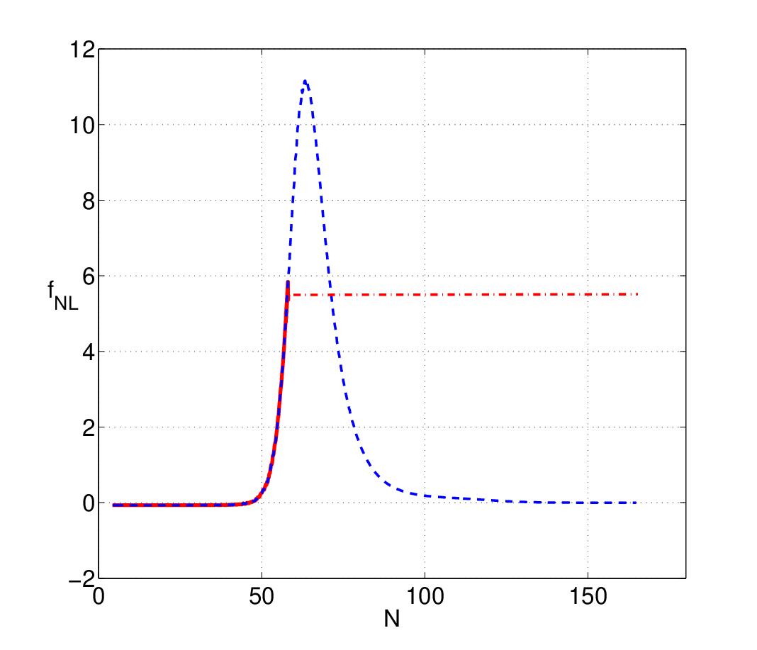
In Fig. 1 we plot the evolution of for , and initial conditions , . We adjust the remaining parameters so that the waterfall occurs when and takes much less than a Hubble time to complete. The blue dotted line represents the generated by the slow-roll fields, ignoring the waterfall. If inflation fails to terminate on the spike this leads to a negligible asymptotic bispectrum. The potential is of ‘valley’ type with , for which the analysis of §3 explains the positive spike. Beginning from there is rapid growth to a positive peak, followed by a softer decay. The peak value is well approximated by Eq. (3.18) which yields . By varying the initial conditions, we have confirmed that the peak value scales approximately as , as predicted by (3.18).
The solid red line represents a numerical evolution, terminated by a waterfall transition on the growing arm of the spike. In the early stages, the numerical results follow the analytic prediction. We continue the calculation past the end of inflation by allowing the waterfall field to become operative. Care must be taken in modelling this transition. We give the waterfall field a small value consistent with the typical RMS value expected from quantum mechanical excitations of a massive field in de Sitter, , where is representative of the waterfall mass before the transition. The results are extremely insensitive to its precise value.55 5 In reality, this RMS value is made up of many inhomogeneous short scale modes. Their collective evolution approximates that of a homogeneous mode, at least in the initial stages before the minimum is reached [83]. We expect this approximation captures at least some of the physics which occurs at the hybrid transition.
The hybrid field is heavy at horizon crossing and is therefore unperturbed. Hence, we need not differentiate with respect to . Using these assumptions, we find that appears to be conserved through the hybrid transition (see Fig. 1). The numerical evolution is only continued for a fraction of an e-fold after the transition, during which time does evolve due to oscillation of the primary fields. However, the resulting oscillations in are decaying and are centred around a fixed value. This behaviour is apparently generic for a range of parameter values, provided the transition happens sufficiently rapidly—in less than an e-fold. One must already impose this “rapid transition” condition to avoid issues with primordial black holes [83].66 6 Note that when the hybrid transition does not occur on a uniform density hypersurface a significant extra contribution to can be generated [81, 82]. We have checked a small number of these cases numerically and find agreement with the formulae given in Ref. [66], although we have only considered examples of positive curvature rather than ridges.
5.1.2 Large non-Gaussianity at the natural adiabatic limit
We illustrate this case using a model closely related to the -axion model of Kim et al. [43], in which the potential is taken to be . The sum is taken over a large number of uncoupled axions, and is the decay constant for the axion. We will study further examples of this type in §5.2. In Ref. [43], many axions were invoked to generate a phase of assisted inflation. Because the potential is sum-separable, the perturbations can be calculated at the adiabatic limit using (4.1) after dropping the -term provided inflation ends when the final field gracefully exits from slow-roll. Whether this occurs depends on the number of fields and the choice of . Taking for all and supposing that the initial conditions are chosen so that only a small number of fields populate the hilltop region near , the asymptotic can be calculated using (4.8). It will typically be moderate or large.
In this section we study a related two-field model. Dynamically, the large number of axions which begin away from the hilltop region serve only to source the Hubble rate. The single field closest to the hilltop sources the non-Gaussianity. (This model has some similarity to the scenario of Boubekeur & Lyth [84].) Therefore, most of the axions can be replaced by a single effective field with a quadratic potential, retaining the full cosine only for the axion closest to the hilltop,
| (5.2) |
where and are constants.
Near the hilltop, the axion potential approximately satisfies . This yields a tachyonic mass . Adjusting the potential if necessary to ensure that remains light at horizon crossing, the mass induces a large via (4.8).
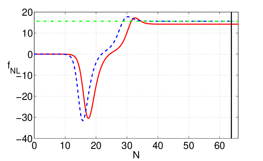
In Figs. 2 and 3 we show a numerical evolution for two choices of parameters. In Fig. 2 we take and , which makes the mass of the axion five times greater than the mass of . The initial conditions are and . As a consequence of its large mass, the axion rolls off the ridge quite early. Therefore the system evolves to the limiting trajectory long before the end of inflation. According to §3, departure from the ridge should produce a large negative spike. Later, convergence into the minimum should produce a positive spike, perhaps followed by a plateau. Finally, as the isocurvature modes are exhausted, the system should evolve to the adiabatic limit (4.8). These features are clearly visible in Fig. 2. Matching the potential (5.2) to the analysis of §3 and using Eq. (3.9), we expect the negative peak of to occur at . This gives good agreement with the observed value. By varying the intial conditions we have verified that scaling with is reproduced to a good approximation. In this case the difference between our slow-roll analysis and the full numerical calculation is at the level of a few percent, consistent with the accuracy of the slow-roll approximation.
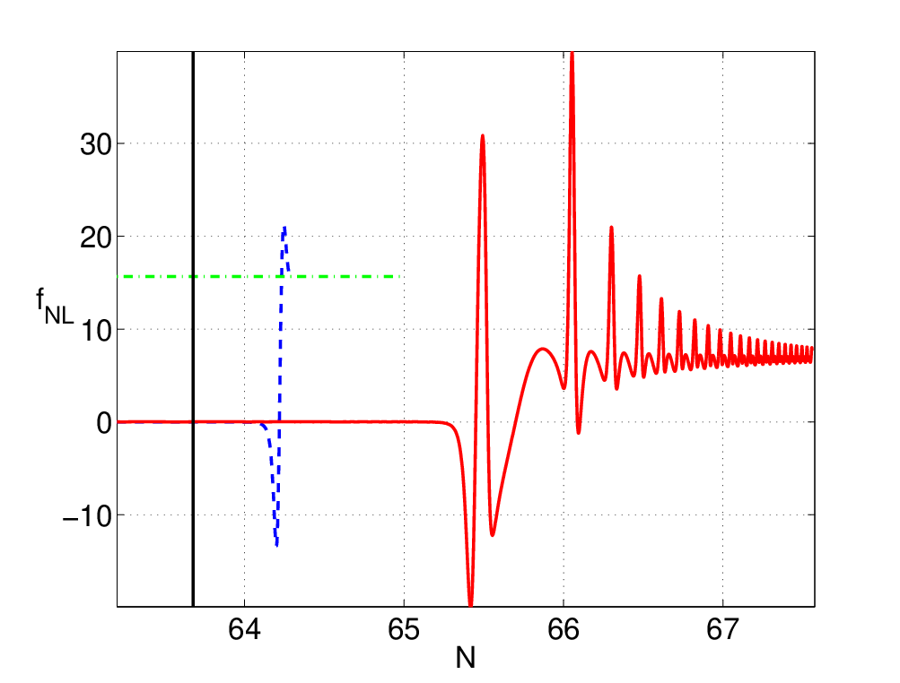
In the second example we take and , giving both fields the same mass. In this case the axion starts to evolve only near the end of inflation, where is approaching the minimum. Indeed, much of its evolution takes place while is oscillating. In these circumstances the adiabatic limit cannot be calculated analytically using (4.1). Nevertheless, the important features can still be understood. While is oscillating in the minimum, its potential energy contributes to the energy density in a way not accounted for by the slow-roll approximation. If we suppose the oscillations do not lead to rapid reheating or preheating, we may expect to approach a constant as the trajectories settle in the minimim and Hubble friction drains their energy. The results are given in Fig. 3. In this simple example, oscillates around an asymptotic value which is lower than would be expected if the adiabatic limit were reached during inflation. In more sophisticated examples, where complex dynamical behaviour can occur during the oscillating phase, it would be necessary to follow their decay in precise detail [85, 86, 87, 88, 89, 90, 91].
This example is representative of a class of model where natural focusing occurs—in this case, caused simply by Hubble damping—but does so only after the slow-roll assumption is violated. There are other models in this class which lead to a large non-Gaussianity at the natural adiabatic limit, such as models which possess an inflection point in their potential with a very slight gradient. We intend to return to these cases in future work [92].
5.1.3 Models with no reconvergence in field space
The third possibility discussed in §1 occurs when the trajectories disperse in field-space but the potential provides no region which would enable them to refocus. An example is provided by the model
| (5.3) |
which was introduced by Byrnes et al. [65]. The dynamics were followed only until the end of slow-roll, at which time the non-Gaussianity was indeed large. However, at this point, the isocurvature modes were not exhausted and the curvature perturbation was still evolving. To study this model, we make the the same parameter choices as Byrnes et al., setting , and [65].
The initial stage is descent from a ridge, and therefore we expect to approach negative values. This is confirmed in Figs. 4 and 5. As the bundle rolls along the ridge (defined by ), we find that Eq. (3.9) gives , in good agreement with the first negative peak in . We have confirmed that the expected scaling with initial conditions is approximately respected.
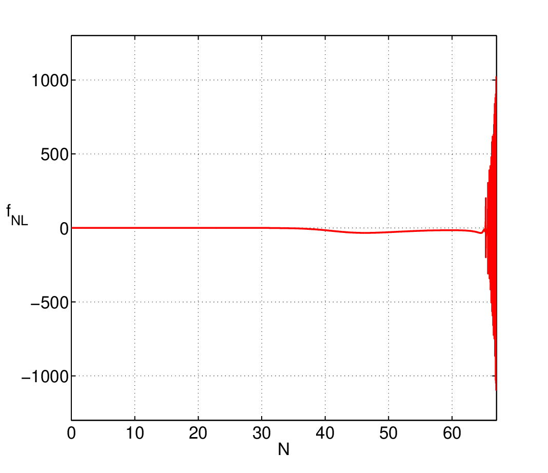
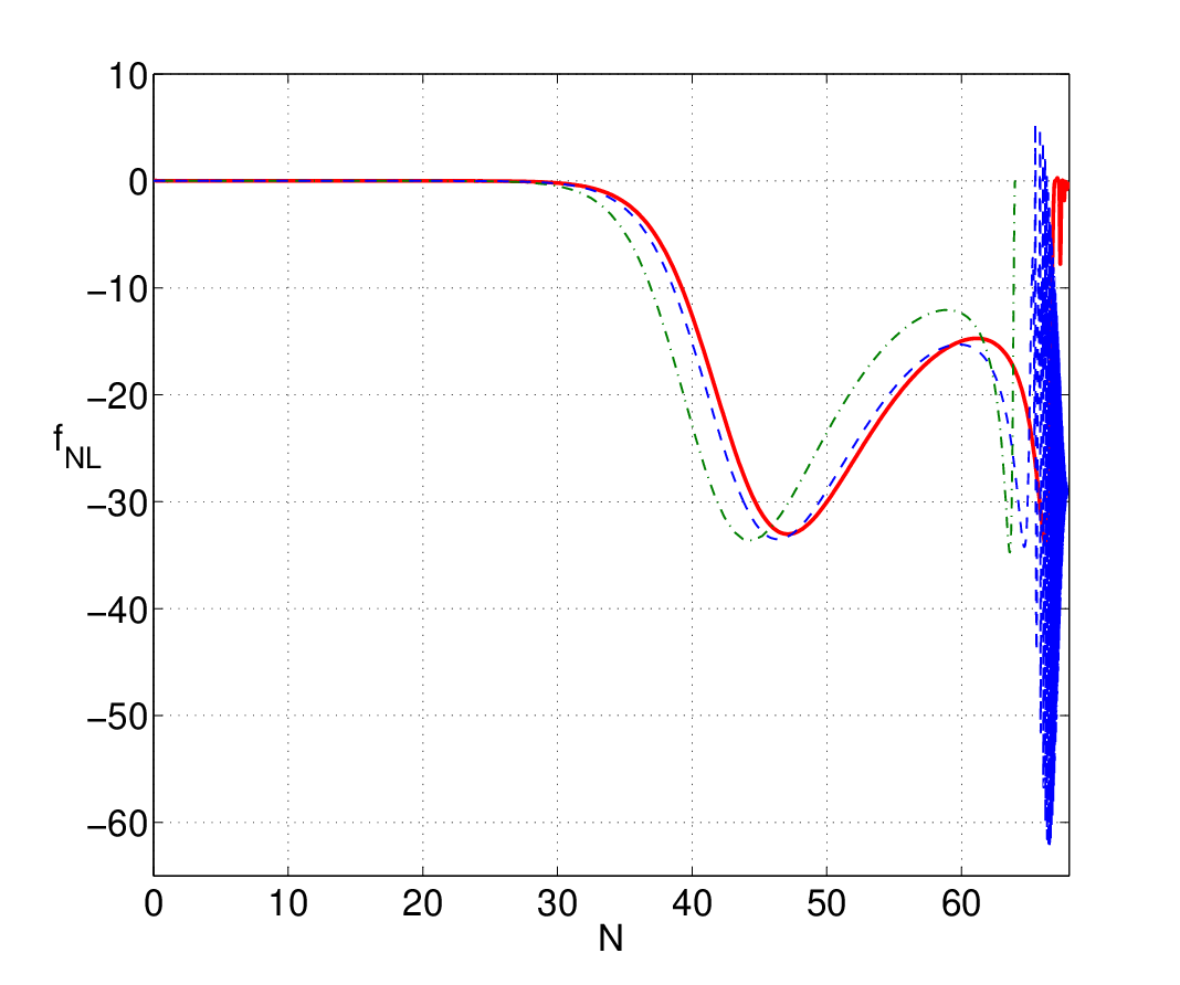
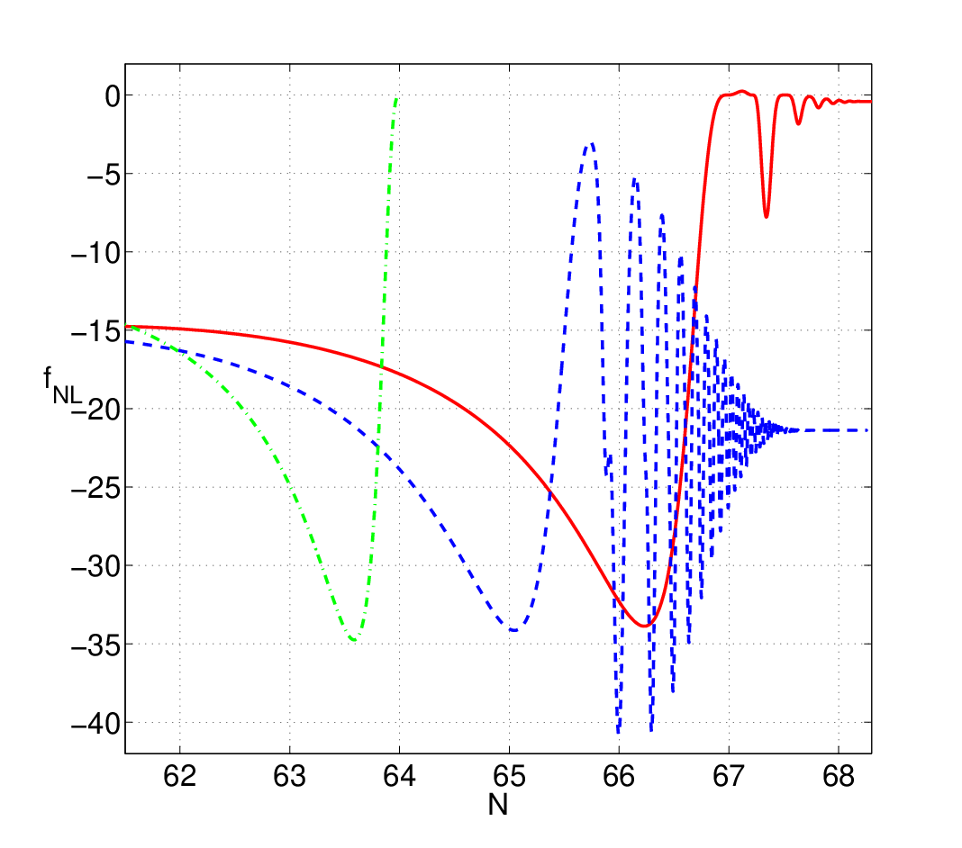
With this choice of parameters, a large is still present as slow-roll breaks down. But because no limiting trajectory is available, continues to evolve—and subsequently oscillates wildly, as the fields oscillate about the line . This does not represent a stable attractor: is a degenerate vacuum, and the field evolves only along the direction during the oscillations. To reach an adiabatic limit we must apply a prescription for reheating. Here, we adopt a very simple perturbative model in which energy is transferred from the field into a radiation component. The dynamical equations are
| (5.4a) | ||||
| (5.4b) | ||||
where is energy density of radiation, and the represent the decay rate from species . We illustrate the effect of reheating in Fig. 5. The final value of is sensitive to the choice of , and hence the time-scale of reheating. We take for all , making reheating begin approximately when and take place on a uniform density hypersurface. A more complicated prescription leads to strong secondary effects which radically alter the value or sign of . After reheating, if the radiation is the only contribution to the energy density, then the statistics of at this time will be the ones relevant for observation. Fig. 5 indicates that these will depend on microphysical details of the reheating phase, at least through , but a systematic understanding is not yet in place.
Our aim has not been to present a realistic model. Rather, we wish to demonstrate that, if no attractor exists within the inflationary regime, we must follow the dynamics until all observable quantities stop evolving at the adiabatic limit. We can expect the asymptotic value of each observable to be sensitive to this evolution, including the time scale and details of reheating.
5.2 -field models
Similar results naturally apply in models with a larger number of fields. In this section we study the model of Kim et al. [43] involving many axion fields self-interacting though the potentials
| (5.5) |
Where the parameters and take common values and for each species, and , this generates naturally large at the adiabatic limit. Although larger can naïvely be obtained by decreasing the , it is necessary to simultaneously increase the number of fields in order to obtain sufficient inflation. There is another difficulty. As the decrease, the approach of to its asymptotic limit occurs later in the evolution. In Fig. 6 we show one realization of this behaviour for and , with initial conditions for the fields randomly distributed in the range . The slow-roll phase ends at latest when , marked by the vertical black line. The evolution to the right of this line is not trustworthy and should be replaced by a numerical calculation. Unfortunately, owing to the large number of fields we have not been able to perform a non-slow roll analysis due to the prohibitive running time of the computation.

There is a specific case where this model can be related exactly to the two-field axion-plus-quadratic model of the the previous section: when fields are initially close to the minimum of the axion potential ( for ) with identical initial conditions, and one field is initially close to its maximum, . In this case the fields act like a large number of fields with a quadratic potential. When they all evolve from an identical initial condition, the dynamics of the many fields is completely identical to the dynamics of a single field , with a quadratic potential of the same mass as the individual fields. For , this reduces identically to the second of the two-field axion-plus-quadratic cases studied in §5.1.2. (See Fig. 3.)
Finally, it is interesting to note that the -field axion model—for which a large follows from relatively generic initial conditions—is closely related to a two-field model in which generation of large apparently requires significant fine-tuning. The tuning appears less dramatic in the original -field model. It is interesting to conjecture that the fine-tuning of initial conditions required to give large in two-field models may be reduced in models with many fields.
6 Conclusions
We have studied the evolution of non-Gaussianity in multiple-field models of inflation. Unless all isocurvature modes become exhausted before the end of inflation, we find that there need not be a unique prediction for . Instead, the final value can depend on independent details, such as the microphysics of a reheating or preheating phase. Where the trajectories naturally focus—for example, if inflation ends with all fields settling into a minimum of the potential—numerical calculations are typically required to determine the precise asymptotic value for . If there is no natural focusing region then numerical calculations and a prescription for reheating will be required. This confirms the natural expectation that analytic predictions [38, 40, 39, 75] are reliable only if the flow of power from isocurvature to curvature modes is quenched before the end of the slow-roll phase.
If an adiabatic limit is reached without passage through a natural focusing region, perhaps by invoking a waterfall transition, then this may occur when the value of is transiently large. However, we caution that although our numerical calculations indicate that can sometimes be preserved through a hybrid transition, there does not yet appear to be a precise characterization of the conditions required for this to occur. Also, whether the end-point of the waterfall is an adiabatic limit may be model dependent. Temporarily ignoring these subtleties, we have shown that descent from a ridge or convergence into a valley can result in a significant, dynamical but transient enhancement of . The two cases are distinguished by a different sign of the resulting , which is inherited from the local parameter.
We have verified that it is possible to construct sum-separable models which exhibit large even when the adiabatic limit is reached during slow-roll inflation. Therefore there is no correlation between large at the end of inflation and the presence of an inexhausted isocurvature perturbation, as has occasionally been suggested. On the other hand, we have demonstrated that this is impossible for product separable cases, where is always of order the slow-roll parameters at horizon crossing.
Among the models we have studied is a new two-field model related to the -field axion model [43]. This exhibits large at the adiabatic limit when this limit is reached before the breakdown of slow-roll. In addition, inflation can end gracefully rather than through a sudden transition. As far as we are aware, this is the first example of such behaviour in the two-field context. This model explicitly illustrates that predictions of the -axion model may be modified if a full numerical calculation for a sufficiently large number of fields could be performed.
Acknowledgments
We would like to thank Chris Byrnes, Andrew Liddle and Karim Malik for helpful discussions. JE is supported by a Science and Technology Facilities Council Studentship. DJM is supported by the Science and Technology Facilities Council grant ST/H002855/1. DS was supported by the Science and Technology Facilities Council [grant numbers ST/F002858/1 and ST/I000976/1].
Appendix A Detailed calculations for separable potentials
A.1 Calculating
Under the assumption of slow-roll and monotonicity (), the number of e-folds can be written with the field as a time variable. Taking the functional derivative of this integral generates three components—two “boundary terms” evaluated on the initial (‘’) and final (‘’) slices, and a “path term”,
| (A.1) |
The summation convention is not used. Physical quantities are independent of , which may be chosen arbitrarily. Employing the notation and , where are dimensionless, we restrict attention to potentials of the form and , where and are arbitrary functions. We refer to these as sum- and product-separable potentials respectively.
For the product-separable potential we evaluate the path term and the final boundary term in Eq. (A.1). Using the slow-roll parameters and also defining we find
| (A.2) |
This applies for arbitrary . Note that any dependence on has disappeared. If the ratio depends on , then the integral requires knowledge of the variation of with . There are at least two cases in which the -dependence is lost: if the integrand is either zero or constant. If the integrand is zero then we have for some constant . This gives the general solution , where the constants and can be absorbed into a redefinition of the potential. This yields
| (A.3) |
If the integrand is constant this implies , where are constants of which and can be eliminated by a further redefinition. We conclude that a general potential yielding a -independent integrand can be expressed as and gives
| (A.4) |
An identical procedure applies to the sum-separable potential, leading to
| (A.5) | |||||
| (A.6) |
A.2 Correspondence between different separable potentials
There is a correspondence between Eqs. (A.5) and (A.3), and between Eqs. (A.6) and (A.4) which was first pointed out by Wang [61] for two field potentials. Redefining turns a potential into a potential, and redefining transforms the potential into the form . Therefore, it is unnecessary to proceed with all four classes of potential. As an independent pair of potentials, we choose and .
A.3 and
To calculate higher-order statistics we require the second derivatives . It proves convenient to introduce new dimensionless slow-roll parameters
| (A.9) | |||||
| (A.10) |
These are elements of a vector and matrix respectively. Note that is diagonal for the product-separable potential and so we rewrite with . A simplification occurs if the limiting trajectory is a straight line in field space, which implies
| (A.11) |
where the vector has elements . If the limiting trajectory lies along the axis, then . In this case, the sign of is given by the mass of the field at horizon crossing but the magnitude is slow-roll suppressed. If we do not make the simplifying assumption that the limiting trajectory is a straight line, then
| (A.12) | |||||
| (A.13) |
For the potential we have . In the simpler situation where is a constant, we find
| (A.14) | |||||
| (A.15) |
Dropping the assumption that is constant leads to additional terms of the form
| (A.16) | |||||
| (A.17) | |||||
| (A.18) |
References
- [1] D. H. Lyth, K. A. Malik, and M. Sasaki, A General proof of the conservation of the curvature perturbation, JCAP 0505 (2005) 004, [arXiv:astro-ph/0411220], [doi:10.1088/1475-7516/2005/05/004].
- [2] J. M. Maldacena, Non-Gaussian features of primordial fluctuations in single field inflationary models, JHEP 0305 (2003) 013, [arXiv:astro-ph/0210603].
- [3] E. J. Copeland, E. W. Kolb, A. R. Liddle, and J. E. Lidsey, Reconstructing the inflation potential, in principle and in practice, Phys.Rev. D48 (1993) 2529–2547, [arXiv:hep-ph/9303288], [doi:10.1103/PhysRevD.48.2529].
- [4] E. J. Copeland, E. W. Kolb, A. R. Liddle, and J. E. Lidsey, Reconstructing the inflaton potential: Perturbative reconstruction to second order, Phys.Rev. D49 (1994) 1840–1844, [arXiv:astro-ph/9308044], [doi:10.1103/PhysRevD.49.1840].
- [5] J. E. Lidsey, A. R. Liddle, E. W. Kolb, E. J. Copeland, T. Barreiro, et al., Reconstructing the inflation potential : An overview, Rev.Mod.Phys. 69 (1997) 373–410, [arXiv:astro-ph/9508078], [doi:10.1103/RevModPhys.69.373].
- [6] J. García-Bellido and D. Wands, Metric perturbations in two field inflation, Phys.Rev. D53 (1996) 5437–5445, [arXiv:astro-ph/9511029], [doi:10.1103/PhysRevD.53.5437].
- [7] G. Rigopoulos and E. Shellard, The separate universe approach and the evolution of nonlinear superhorizon cosmological perturbations, Phys.Rev. D68 (2003) 123518, [arXiv:astro-ph/0306620], [doi:10.1103/PhysRevD.68.123518].
- [8] D. Langlois and F. Vernizzi, Evolution of non-linear cosmological perturbations, Phys.Rev.Lett. 95 (2005) 091303, [arXiv:astro-ph/0503416], [doi:10.1103/PhysRevLett.95.091303].
- [9] D. Langlois and F. Vernizzi, Conserved non-linear quantities in cosmology, Phys.Rev. D72 (2005) 103501, [arXiv:astro-ph/0509078], [doi:10.1103/PhysRevD.72.103501].
- [10] D. Langlois and F. Vernizzi, Nonlinear perturbations for dissipative and interacting relativistic fluids, JCAP 0602 (2006) 014, [arXiv:astro-ph/0601271], [doi:10.1088/1475-7516/2006/02/014].
- [11] D. Langlois, F. Vernizzi, and D. Wands, Non-linear isocurvature perturbations and non-Gaussianities, JCAP 0812 (2008) 004, [arXiv:0809.4646], [doi:10.1088/1475-7516/2008/12/004].
- [12] D. Langlois and F. Vernizzi, A geometrical approach to nonlinear perturbations in relativistic cosmology, Class.Quant.Grav. 27 (2010) 124007, [arXiv:1003.3270], [doi:10.1088/0264-9381/27/12/124007].
- [13] A. J. Christopherson and K. A. Malik, The non-adiabatic pressure in general scalar field systems, Phys.Lett. B675 (2009) 159–163, [arXiv:0809.3518], [doi:10.1016/j.physletb.2009.04.003].
- [14] A. Naruko and M. Sasaki, Conservation of the nonlinear curvature perturbation in generic single-field inflation, Class.Quant.Grav. 28 (2011) 072001, [arXiv:1101.3180], [doi:10.1088/0264-9381/28/7/072001].
- [15] X. Gao, Conserved cosmological perturbation in Galileon models, arXiv:1106.0292.
- [16] J. Khoury and F. Piazza, Rapidly-Varying Speed of Sound, Scale Invariance and Non-Gaussian Signatures, JCAP 0907 (2009) 026, [arXiv:0811.3633], [doi:10.1088/1475-7516/2009/07/026].
- [17] D. Baumann, L. Senatore, and M. Zaldarriaga, Scale-Invariance and the Strong Coupling Problem, arXiv:1101.3320.
- [18] S. Weinberg, Can non-adiabatic perturbations arise after single-field inflation?, Phys.Rev. D70 (2004) 043541, [arXiv:astro-ph/0401313], [doi:10.1103/PhysRevD.70.043541].
- [19] S. Weinberg, Must cosmological perturbations remain non-adiabatic after multi-field inflation?, Phys.Rev. D70 (2004) 083522, [arXiv:astro-ph/0405397], [doi:10.1103/PhysRevD.70.083522].
- [20] S. Weinberg, Non-Gaussian Correlations Outside the Horizon, Phys.Rev. D78 (2008) 123521, [arXiv:0808.2909], [doi:10.1103/PhysRevD.78.123521].
- [21] S. Weinberg, Non-Gaussian Correlations Outside the Horizon II: The General Case, Phys.Rev. D79 (2009) 043504, [arXiv:0810.2831], [doi:10.1103/PhysRevD.79.043504].
- [22] C. L. Bennett et al., Cosmic temperature fluctuations from two years of COBE differential microwave radiometers observations, Astrophys. J. 436 (1994) 423–442, [arXiv:astro-ph/9401012], [doi:10.1086/174918].
- [23] C. L. Bennett et al., 4-Year COBE DMR Cosmic Microwave Background Observations: Maps and Basic Results, Astrophys. J. 464 (1996) L1–L4, [arXiv:astro-ph/9601067], [doi:10.1086/310075].
- [24] E. Komatsu and D. N. Spergel, Acoustic signatures in the primary microwave background bispectrum, Phys.Rev. D63 (2001) 063002, [arXiv:astro-ph/0005036], [doi:10.1103/PhysRevD.63.063002].
- [25] N. Kogo and E. Komatsu, Angular trispectrum of CMB temperature anisotropy from primordial non-gaussianity with the full radiation transfer function, Phys.Rev. D73 (2006) 083007, [arXiv:astro-ph/0602099], [doi:10.1103/PhysRevD.73.083007].
- [26] M. Alishahiha, E. Silverstein, and D. Tong, DBI in the sky, Phys.Rev. D70 (2004) 123505, [arXiv:hep-th/0404084], [doi:10.1103/PhysRevD.70.123505].
- [27] N. Arkani-Hamed, P. Creminelli, S. Mukohyama, and M. Zaldarriaga, Ghost inflation, JCAP 0404 (2004) 001, [arXiv:hep-th/0312100], [doi:10.1088/1475-7516/2004/04/001].
- [28] D. H. Lyth and Y. Rodríguez, The Inflationary prediction for primordial non-Gaussianity, Phys.Rev.Lett. 95 (2005) 121302, [arXiv:astro-ph/0504045], [doi:10.1103/PhysRevLett.95.121302].
- [29] D. H. Lyth, Generating the curvature perturbation at the end of inflation, JCAP 0511 (2005) 006, [arXiv:astro-ph/0510443], [doi:10.1088/1475-7516/2005/11/006].
- [30] D. H. Lyth and D. Wands, Generating the curvature perturbation without an inflaton, Phys.Lett. B524 (2002) 5–14, [arXiv:hep-ph/0110002], [doi:10.1016/S0370-2693(01)01366-1].
- [31] T. Moroi and T. Takahashi, Effects of cosmological moduli fields on cosmic microwave background, Phys.Lett. B522 (2001) 215–221, [arXiv:hep-ph/0110096], [doi:10.1016/S0370-2693(01)01295-3, 10.1016/S0370-2693(01)01295-3].
- [32] G. Dvali, A. Gruzinov, and M. Zaldarriaga, A new mechanism for generating density perturbations from inflation, Phys.Rev. D69 (2004) 023505, [arXiv:astro-ph/0303591], [doi:10.1103/PhysRevD.69.023505].
- [33] M. Zaldarriaga, Non-Gaussianities in models with a varying inflaton decay rate, Phys.Rev. D69 (2004) 043508, [arXiv:astro-ph/0306006], [doi:10.1103/PhysRevD.69.043508].
- [34] D. Seery and J. E. Lidsey, Primordial non-Gaussianities from multiple-field inflation, JCAP 0509 (2005) 011, [arXiv:astro-ph/0506056], [doi:10.1088/1475-7516/2005/09/011].
- [35] D. Seery, J. E. Lidsey, and M. S. Sloth, The inflationary trispectrum, JCAP 0701 (2007) 027, [arXiv:astro-ph/0610210], [doi:10.1088/1475-7516/2007/01/027].
- [36] D. Seery, M. S. Sloth, and F. Vernizzi, Inflationary trispectrum from graviton exchange, JCAP 0903 (2009) 018, [arXiv:0811.3934], [doi:10.1088/1475-7516/2009/03/018].
- [37] S. Dimopoulos, S. Kachru, J. McGreevy, and J. G. Wacker, N-flation, JCAP 0808 (2008) 003, [arXiv:hep-th/0507205], [doi:10.1088/1475-7516/2008/08/003].
- [38] L. Alabidi and D. H. Lyth, Inflation models and observation, JCAP 0605 (2006) 016, [arXiv:astro-ph/0510441], [doi:10.1088/1475-7516/2006/05/016].
- [39] F. Vernizzi and D. Wands, Non-gaussianities in two-field inflation, JCAP 0605 (2006) 019, [arXiv:astro-ph/0603799], [doi:10.1088/1475-7516/2006/05/019].
- [40] L. Alabidi, Non-gaussianity for a Two Component Hybrid Model of Inflation, JCAP 0610 (2006) 015, [arXiv:astro-ph/0604611], [doi:10.1088/1475-7516/2006/10/015].
- [41] S. A. Kim and A. R. Liddle, Nflation: multi-field inflationary dynamics and perturbations, Phys.Rev. D74 (2006) 023513, [arXiv:astro-ph/0605604], [doi:10.1103/PhysRevD.74.023513].
- [42] S. A. Kim and A. R. Liddle, Nflation: Non-Gaussianity in the horizon-crossing approximation, Phys.Rev. D74 (2006) 063522, [arXiv:astro-ph/0608186], [doi:10.1103/PhysRevD.74.063522].
- [43] S. A. Kim, A. R. Liddle, and D. Seery, Non-gaussianity in axion Nflation models, Phys.Rev.Lett. 105 (2010) 181302, [arXiv:1005.4410], [doi:10.1103/PhysRevLett.105.181302].
- [44] J. Meyers and N. Sivanandam, Non-Gaussianities in Multifield Inflation: Superhorizon Evolution, Adiabaticity, and the Fate of , arXiv:1011.4934.
- [45] J. Meyers and N. Sivanandam, Adiabaticity and the Fate of Non-Gaussianities: The Trispectrum and Beyond, arXiv:1104.5238.
- [46] D. Lyth, Large Scale Energy Density Perturbations and Inflation, Phys.Rev. D31 (1985) 1792–1798, [doi:10.1103/PhysRevD.31.1792].
- [47] J. M. Bardeen, P. J. Steinhardt, and M. S. Turner, Spontaneous Creation of Almost Scale-Free Density Perturbations in an Inflationary Universe, Phys.Rev. D28 (1983) 679, [doi:10.1103/PhysRevD.28.679].
- [48] D. Wands, K. A. Malik, D. H. Lyth, and A. R. Liddle, A new approach to the evolution of cosmological perturbations on large scales, Phys. Rev. D62 (2000) 043527, [arXiv:astro-ph/0003278], [doi:10.1103/PhysRevD.62.043527].
- [49] L. Senatore and M. Zaldarriaga, On Loops in Inflation, JHEP 1012 (2010) 008, [arXiv:0912.2734], [doi:10.1007/JHEP12(2010)008].
- [50] N. Bartolo, S. Matarrese, M. Pietroni, A. Riotto, and D. Seery, On the Physical Significance of Infra-red Corrections to Inflationary Observables, JCAP 0801 (2008) 015, [arXiv:0711.4263], [doi:10.1088/1475-7516/2008/01/015].
- [51] D. Seery, A parton picture of de Sitter space during slow-roll inflation, JCAP 0905 (2009) 021, [arXiv:0903.2788], [doi:10.1088/1475-7516/2009/05/021].
- [52] D. Seery, Infrared effects in inflationary correlation functions, Class.Quant.Grav. 27 (2010) 124005, [arXiv:1005.1649], [doi:10.1088/0264-9381/27/12/124005].
- [53] A. Rajaraman, J. Kumar, and L. Leblond, Constructing Infrared Finite Propagators in Inflating Space-time, Phys.Rev. D82 (2010) 023525, [arXiv:1002.4214], [doi:10.1103/PhysRevD.82.023525].
- [54] Y. Urakawa and T. Tanaka, Natural selection of inflationary vacuum required by infra-red regularity and gauge-invariance, arXiv:1009.2947.
- [55] D. H. Lyth, Non-gaussianity and cosmic uncertainty in curvaton-type models, JCAP 0606 (2006) 015, [arXiv:astro-ph/0602285], [doi:10.1088/1475-7516/2006/06/015].
- [56] D. Salopek, Characteristics of cosmic time, Phys.Rev. D52 (1995) 5563–5575, [arXiv:astro-ph/9506146], [doi:10.1103/PhysRevD.52.5563].
- [57] S. Hawking, Perturbations of an expanding universe, Astrophys.J. 145 (1966) 544–554, [doi:10.1086/148793].
- [58] A. A. Starobinsky, Dynamics of Phase Transition in the New Inflationary Universe Scenario and Generation of Perturbations, Phys.Lett. B117 (1982) 175–178, [doi:10.1016/0370-2693(82)90541-X].
- [59] A. A. Starobinsky, Multicomponent de Sitter (Inflationary) Stages and the Generation of Perturbations, JETP Lett. 42 (1985) 152–155.
- [60] M. Sasaki and E. D. Stewart, A General analytic formula for the spectral index of the density perturbations produced during inflation, Prog.Theor.Phys. 95 (1996) 71–78, [arXiv:astro-ph/9507001], [doi:10.1143/PTP.95.71].
- [61] T. Wang, Note on Non-Gaussianities in Two-field Inflation, Phys.Rev. D82 (2010) 123515, [arXiv:1008.3198], [doi:10.1103/PhysRevD.82.123515].
- [62] D. H. Lyth and I. Zaballa, A Bound concerning primordial non-Gaussianity, JCAP 0510 (2005) 005, [arXiv:astro-ph/0507608], [doi:10.1088/1475-7516/2005/10/005].
- [63] M. Sasaki, Multi-brid inflation and non-Gaussianity, Prog.Theor.Phys. 120 (2008) 159–174, [arXiv:0805.0974], [doi:10.1143/PTP.120.159].
- [64] A. Naruko and M. Sasaki, Large non-Gaussianity from multi-brid inflation, Prog.Theor.Phys. 121 (2009) 193–210, [arXiv:0807.0180], [doi:10.1143/PTP.121.193].
- [65] C. T. Byrnes, K.-Y. Choi, and L. M. Hall, Conditions for large non-Gaussianity in two-field slow-roll inflation, JCAP 0810 (2008) 008, [arXiv:0807.1101], [doi:10.1088/1475-7516/2008/10/008].
- [66] C. T. Byrnes, K.-Y. Choi, and L. M. Hall, Large non-Gaussianity from two-component hybrid inflation, JCAP 0902 (2009) 017, [arXiv:0812.0807], [doi:10.1088/1475-7516/2009/02/017].
- [67] D. J. Mulryne, D. Seery, and D. Wesley, Moment transport equations for non-Gaussianity, JCAP 1001 (2010) 024, [arXiv:0909.2256], [doi:10.1088/1475-7516/2010/01/024].
- [68] D. J. Mulryne, D. Seery, and D. Wesley, Moment transport equations for the primordial curvature perturbation, arXiv:1008.3159.
- [69] C. M. Peterson and M. Tegmark, Non-Gaussianity in Two-Field Inflation, arXiv:1011.6675.
- [70] D. H. Lyth, The contribution of the hybrid inflation waterfall to the primordial curvature perturbation, arXiv:1012.4617.
- [71] J. Fonseca, M. Sasaki, and D. Wands, Large-scale Perturbations from the Waterfall Field in Hybrid Inflation, JCAP 1009 (2010) 012, [arXiv:1005.4053], [doi:10.1088/1475-7516/2010/09/012].
- [72] A. A. Abolhasani and H. Firouzjahi, No Large Scale Curvature Perturbations during Waterfall of Hybrid Inflation, Phys.Rev. D83 (2011) 063513, [arXiv:1005.2934], [doi:10.1103/PhysRevD.83.063513].
- [73] J.-O. Gong and M. Sasaki, Waterfall field in hybrid inflation and curvature perturbation, JCAP 1103 (2011) 028, [arXiv:1010.3405], [doi:10.1088/1475-7516/2011/03/028].
- [74] D. Mulryne, D. Seery, and D. Wesley, Non-Gaussianity constrains hybrid inflation, arXiv:0911.3550.
- [75] T. Battefeld and R. Easther, Non-Gaussianities in Multi-field Inflation, JCAP 0703 (2007) 020, [arXiv:astro-ph/0610296], [doi:10.1088/1475-7516/2007/03/020].
- [76] K.-Y. Choi, L. M. Hall, and C. van de Bruck, Spectral Running and Non-Gaussianity from Slow-Roll Inflation in Generalised Two-Field Models, JCAP 0702 (2007) 029, [arXiv:astro-ph/0701247], [doi:10.1088/1475-7516/2007/02/029].
- [77] D. Battefeld and T. Battefeld, On Non-Gaussianities in Multi-Field Inflation (N fields): Bi- and Tri-spectra beyond Slow-Roll, JCAP 0911 (2009) 010, [arXiv:0908.4269], [doi:10.1088/1475-7516/2009/11/010].
- [78] C. T. Byrnes and G. Tasinato, Non-Gaussianity beyond slow roll in multi-field inflation, JCAP 0908 (2009) 016, [arXiv:0906.0767], [doi:10.1088/1475-7516/2009/08/016].
- [79] A. R. Liddle, A. Mazumdar, and F. E. Schunck, Assisted inflation, Phys. Rev. D58 (1998) 061301, [arXiv:astro-ph/9804177], [doi:10.1103/PhysRevD.58.061301].
- [80] A. M. Green and J. E. Lidsey, Generalized compactification and assisted dynamics of multiscalar field cosmologies, Phys.Rev. D61 (2000) 067301, [arXiv:astro-ph/9907223], [doi:10.1103/PhysRevD.61.067301].
- [81] L. Alabidi and D. Lyth, Curvature perturbation from symmetry breaking the end of inflation, JCAP 0608 (2006) 006, [arXiv:astro-ph/0604569], [doi:10.1088/1475-7516/2006/08/006].
- [82] Q.-G. Huang, A Geometric description of the non-Gaussianity generated at the end of multi-field inflation, JCAP 0906 (2009) 035, [arXiv:0904.2649], [doi:10.1088/1475-7516/2009/06/035].
- [83] J. Garcia-Bellido, A. D. Linde, and D. Wands, Density perturbations and black hole formation in hybrid inflation, Phys. Rev. D54 (1996) 6040–6058, [arXiv:astro-ph/9605094], [doi:10.1103/PhysRevD.54.6040].
- [84] L. Boubekeur and D. Lyth, Detecting a small perturbation through its non-Gaussianity, Phys.Rev. D73 (2006) 021301, [arXiv:astro-ph/0504046], [doi:10.1103/PhysRevD.73.021301].
- [85] J. H. Traschen and R. H. Brandenberger, Particle production during out-of-equilibrium phase transitions, Phys.Rev. D42 (1990) 2491–2504, [doi:10.1103/PhysRevD.42.2491].
- [86] L. Kofman, A. D. Linde, and A. A. Starobinsky, Reheating after inflation, Phys. Rev. Lett. 73 (1994) 3195–3198, [arXiv:hep-th/9405187], [doi:10.1103/PhysRevLett.73.3195].
- [87] Y. Shtanov, J. H. Traschen, and R. H. Brandenberger, Universe reheating after inflation, Phys.Rev. D51 (1995) 5438–5455, [arXiv:hep-ph/9407247], [doi:10.1103/PhysRevD.51.5438].
- [88] A. Chambers and A. Rajantie, Lattice calculation of non-Gaussianity from preheating, Phys.Rev.Lett. 100 (2008) 041302, [arXiv:0710.4133], [doi:10.1103/PhysRevLett.100.041302, 10.1103/PhysRevLett.100.041302].
- [89] A. Chambers and A. Rajantie, Non-Gaussianity from massless preheating, JCAP 0808 (2008) 002, [arXiv:0805.4795], [doi:10.1088/1475-7516/2008/08/002].
- [90] J. Bond, A. V. Frolov, Z. Huang, and L. Kofman, Non-Gaussian Spikes from Chaotic Billiards in Inflation Preheating, Phys.Rev.Lett. 103 (2009) 071301, [arXiv:0903.3407], [doi:10.1103/PhysRevLett.103.071301].
- [91] K. Kohri, D. H. Lyth, and C. A. Valenzuela-Toledo, Preheating and the non-gaussianity of the curvature perturbation, JCAP 1002 (2010) 023, [arXiv:0904.0793], [doi:10.1088/1475-7516/2010/02/023, 10.1088/1475-7516/2010/09/E01].
- [92] J. Elliston, D. Mulryne, D. Seery, and R. Tavakol, Evolution of non-Gaussianity in multi-scalar field models, arXiv:1107.2270.