Search for conformal invariance in compressible two-dimensional turbulence
Abstract
We present a search for conformal invariance in vorticity isolines of two-dimensional compressible turbulence. The vorticity is measured by tracking the motion of particles that float at the surface of a turbulent tank of water. The three-dimensional turbulence in the tank has a Taylor microscale . The conformal invariance theory being tested here is related to the behavior of equilibrium systems near a critical point. This theory is associated with the work of Löwner, Schramm and others and is usually referred to as Schramm-Löwner Evolution (SLE). The system was exposed to several tests of SLE. The results of these tests suggest that zero-vorticity isolines exhibit noticeable departures from this type of conformal invariance.
Copyright (2011) American Institute of Physics. This article may be downloaded for personal use only. Any other use requires prior permission of the author and the American Institute of Physics. The following article appeared in (Stefanus, J. Larkin, W.I. Goldburg, ”Search for conformal invariance in compressible two-dimensional turbulence,” Phys. of Fluids 23, 105101 (2011)) and may be found at http://link.aip.org/link/?PHF/23/105101.
pacs
go hereI Introduction
Strong turbulence is fiercely difficult to understand because it is dominated by nonlinear effects, and because many degrees of freedom of fluid flow are excited [1]. Some of its main features can be understood from dimensional arguments based on an eddy cascade theory. There is a range of eddy sizes over which the system exhibits approximate self-similarity or scale invariance. Most efforts have been focused on this self-similar range, often called the inertial range. It can span length scales ranging from many meters down to eddy sizes of tens of microns in the atmosphere, in the ocean, and in large wind tunnels.
Though most endeavors are focused on understanding three-dimensional turbulence, two dimensional (2D) flows are important from a practical and fundamental point of view. The depth of oceans (L) and the thickness of the atmosphere is very small compared to the earth’s radius . Large-scale velocity variations are properly viewed as two-dimensional.
Two dimensional turbulence displays striking differences from its 3D counterpart. In 2D, smaller eddies combine to form bigger ones while the reverse happens in three dimensions. This so-called ”inverse cascade” in 2D turbulence characterizes hurricane growth in the troposphere [2].
The theory of two-dimensional (2D) turbulence brings new complications and simplifications at the same time. Between the large eddies in 2D turbulence are thin regions where the vorticity of the flow is very large, even though these regions contain only a small fraction of the turbulent energy. In two dimensions, the vorticity is, of course, perpendicular to the plane of the 2D flow and is hence a scalar. In 3D, the vorticity is amplified by velocity gradients, whereas in 2D, its mean square vorticity is a constant, viscous damping aside. As for this damping, it occurs at small scales and is almost absent in the self-similar range of interest here.
It is obviously important if 2D turbulence should turn out to exhibit invariance features that go beyond self-similarity. Recent theoretical and numerical work suggests that this is so. This evidence comes from the study of contours of zero vorticity in an incompressible flow [3] (to be called BBCF) . In that important paper, the authors focus on the geometry of (contorted) paths through the fluid where the vorticity is zero at each instant of time . Their simulations reveal a new type of conformal invariance. The conformal invariance discussed here , and by BBCF, is unrelated to the usual conformal mapping technique applied to electric potential functions. Rather, it is about the growth of a random curve where each incremental length is produced by a conformal map characterized by a Brownian function.
A path in the plane, written as , is conformally invariant (in this sense [4]), if there is a function that can map the path back to the real axis in the plane while preserving all the angles (See Fig. 1).
The present work is an experimental study of the contours of constant vorticity in a flow. We know of no published experiments for incompressible systems. The present laboratory observations display approximate conformal invariance for the contours of zero vorticity measured at hundreds of instants of time . Contours of nonzero vorticity paths were also examined. Larger deviations from conformal invariance are observed.
It was noted by BBCF that with present technology, it is technically not possible to search for conformal invariance in 2D flow experiments. However, in the compressible flow experiments to be described here, it was possible to accumulate data over a sufficiently wide parameter range to make such a test. In this work, we use an overhead fast camera to track the motion of particles that float on a turbulent tank of water. These particles have a density that is a fourth of the density of water, so their motion is confined to the surface of the underlying turbulent flow, which is, of course three-dimensional. The flow of the turbulent water underneath the floaters is incompressible, assuring that the two-dimensional divergence of the velocity of the floaters is not zero. The particles are small enough to be almost inertia-free. Thus they sample the velocity of the flow in the surface plane , as discussed below. The present experiments are performed at a moderately high Reynolds number where the inertial range is appreciably large.
This system of floaters is very different from conventional two-dimensional turbulence and also from those studied by BBCF. It is not merely that the surface on which the floaters move is rippled (their amplitude is small [5]), it is that the floaters do not form a separate system; they can exchange energy with those water particles beneath them. In principle, at least, they can take and return their kinetic energy to the underlying fluid on all spatial scales. Thus there is no reason to expect an energy cascade which implies dissipation only at small scales or at the boundaries of the container. Nevertheless, the squared velocity difference between pairs of points separated by distances , closely conform to that of 3D turbulence, . This scaling is seen in experiments as well as simulations [5].
The present study hinges on the measurement of a random variable , yet to be defined, whose average mean square must be Brownian in character. In that case
| (1) |
The exponent and the value of are measured in the experiments discussed here.
The parameter is a dimensionless length and not time, and the exponent must be unity, as in Brownian motion, a requirement that must be met if conformal invariance is realized. The dimensionless ”diffusivity” is a very important parameter in the theory being tested here. One may think of as the dimensionless diffusivity, but only if = 1. For a self-avoiding random walk =8/3, and for critical percolation = 6 [4]. This last value is deduced in the simulations of BBCF. In the present experiments, the value of for the zero-vorticity contours was extracted from measurements made at many instants of time. At each instant of time , there are many constant vorticity lines. The parameter increases along each line.
II The search for
The analysis of the experimental data, to be discussed below, requires that the above-defined be uniquely determined by the function (usually referred to as the driving function), which is related to the experimental observations. Thus, also depends on and hence will be written as . Roughly speaking, the dimensionless parameter is proportional to the “length” of the 2D curve, which is being mapped by . This dependence on is what is usually referred to as the Löwner differential equation,
| (2) |
It was O. Schramm who first discovered that for a conformally invariant random curve in a 2D plane, is a one-dimensional Brownian motion obeying Eq. 1 [6]. In this case, the random curve is referred to as a Schramm-Löwner Evolution (SLE) trace. For a more formal and complete discussion of SLE, see [4].
One of the most effective ways to identify this type of conformal invariance is to measure , defined by the above differential equation, and see if its mean square average obeys Eq. 1. In the next two sections, the experiment and the procedure to calculate is described.

A typical SLE trace is shown in Fig. 1. Such traces are both self-similar and self-avoiding. After the conformal transformation, the grid in the plane is rectangular; the transformation under is conformal, as all the angles are preserved.
III Experimental
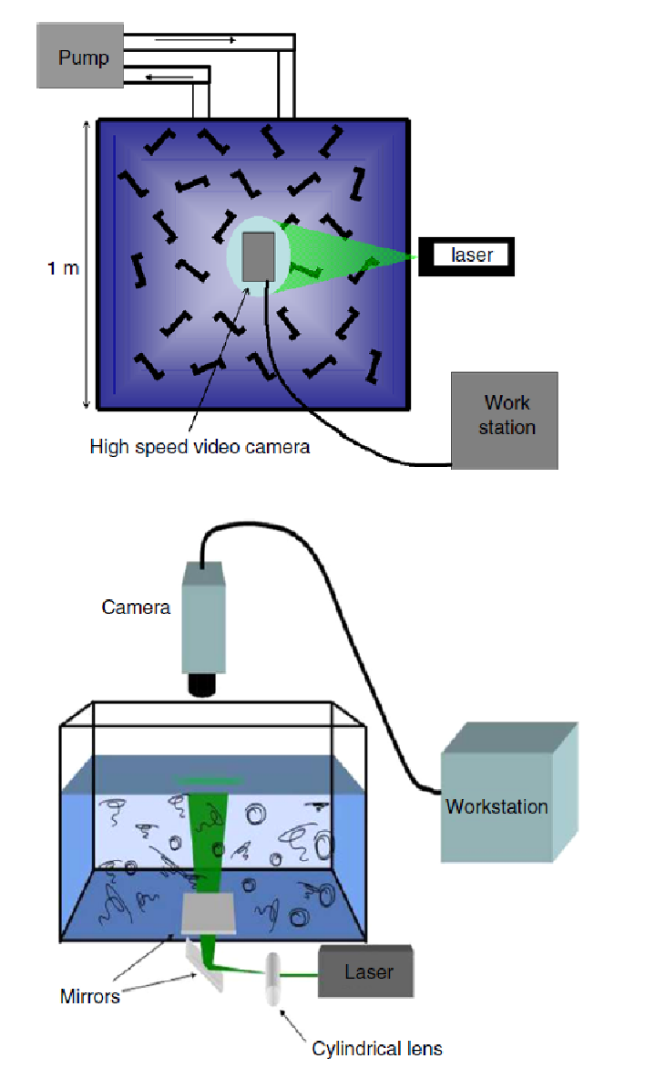
The 1m 1m tank is filled with water to a height of 30 cm. The tank is large compared to the camera’s field of view. The turbulence is generated by a large pump connected to a network of rotating jets in a plane 10 cm above the tank floor. See Fig. 2 for a schematic of the experimental setup. The arrangement creates uniform turbulence in the center of the tank and also moves the source of turbulent injection far from the fluid surface where the measurements are made [5]. With this scheme, surface waves, which cannot be avoided, do not exceed an amplitude of 1 mm [5]. It is necessary that the surface of the tank be freshly cleaned before each set of measurements. Otherwise, amphiphiles form a continuous layer on the surface and prevents the floaters from moving freely under the action of the turbulence [5].
The hydrophilic particles chosen here are subject to capillary forces which are very small compared to forces coming from the turbulence, and do not affect the results as they do in [7, 8]. The non-inertial character of the particles is minimal because the Stokes number is small: [9].
During an experimental run, the floating particles (50 m diameter and specific gravity of 0.25) are constantly seeded into the fluid from the tank floor, where they undergo turbulent mixing as they rise due to buoyancy and are uniformly dispersed by the time they rise to the surface. Once at the free-surface, their motion is constrained to the two-dimensional surface plane. Their motion is tracked with a high-speed camera (Phantom v.5) situated above the tank. The camera field-of-view is a square area of side length L = 9 cm. The constant particle injection is necessary to replace floaters that stick to the tank walls. The sources and sinks at the surface fluctuate in both time and space, which can cause particles to leave the camera’s field of view.
Instantaneous velocity fields are measured using an in-house developed particle imaging velocimetry (PIV) program which processes the recorded images of the floaters. The constant injection of particles ensures that surface sources and sinks receive an adequate coverage of particles on the surface. The local particle density at the surface determines the average spacing of the velocity vector fields produced by the PIV program. The resulting velocity vectors are spaced (on average) by over both sources and sinks , where is the size of the smallest eddies in the inertial range [10].
| Parameter | Symbol used | Measured |
|---|---|---|
| in text | value | |
| Taylor microscale (cm) | 0.37 | |
| Taylor | 160 | |
| Integral scale (cm) | 1.42 | |
| Large Eddy Turnover | 0.43 | |
| Time (LETT) (s) | ||
| Dissipation rate | 6.05 | |
| (cm2/s3) | ||
| Kolmogorov scale (cm) | 0.02 | |
| RMS velocity (cm/s) | 3.3 | |
| Compressibility | 0.49 2% |
Data were taken for several values of with an average . Turbulent parameters measured at the surface are listed in Table 1. All of the statistics presented below were obtained by evolving Lagrangian particles in each frame.
IV Results and Discussion
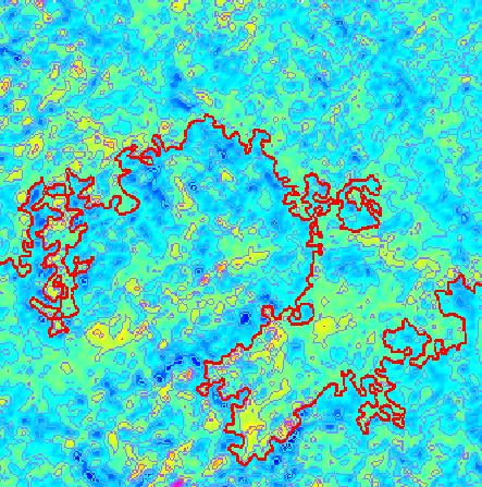

The vorticity field at each point, and at each instant of time , is extracted from a measurement of the velocity field at equally spaced points separated by mm over the 9 cm 9 cm field of view of the camera, giving a resolution of 160 160 points. The camera captures the images at a rate of 133 Hz. The total number of frames that were analyzed is 833.
In each frame there are roughly 1000 vorticity isolines and 400 zero-vorticity lines, see Fig. 3. The vorticity field is approximated using Stoke’s Theorem , where is an area of size . Although for a fractal object the concept of length is not clearly specified, the average length of the longest zero isoline of each frame is roughly 1000 steps, where the step size is .
From each frame, the longest zero and non-zero vorticity lines are extracted. An x-y axis is chosen for each isoline in each frame. The lowest point of the isoline is taken as the origin of the complex plane, because only concerns the upper complex plane, . Next, we calculate the driving function of each of the vorticity isolines using an algorithm implemented by T. Kennedy [11].
Stated briefly, the algorithm goes by decomposing , where maps the curve from 0 to back to the real axis and maps the image of the curve from to under back to the real axis. By recursively decomposing , we get . Each maps one small segment of the curve to the real axis, where has to satisfy Löwner equation (Eq. 2) within each . In principle, we take but in the experiments the smallest is the spatial interval of the two closest points with the same vorticity (). Each incremental map is approximated by a Laurent series around , . This produces a sequence of discrete that approximates the true driving functions .
There are two ways of calculating (Eq. 1). One way is to do self-averaging along followed by an ensemble average over the 833 runs, another way is to calculate the ensemble average over directly as done by BBCF. If is Brownian, as expected of SLE traces, the two methods should yield the same result for and the exponent . The resulting values of and from the two different methods will be denoted and for the self-average and and for the ensemble average.
The self-averaging is done by calculating , where is an average over for each fixed value of . The exponent in Eq. 1 is calculated by taking the log of both sides of the equation, i.e. for each curve and fitting it to a straight line (Fig. 4). The slope of the line is the value of the exponent for that particular curve. The ensemble average over the 833 values of and are then taken to be the value for and for the system.
For SLE, as for Brownian motion, these two methods of averaging should produce the same results. Therefore, an easy way to distinguish vorticity data from effects of random noise follows from comparing results obtained by these two different averaging methods. To illustrate, we simulated SLE traces, and performed this particular test on those traces for a range of -values from 1 to 8 with increments of 0.5. In this simulation, there are 1000 SLE traces for each value of ; each trace contains 4000 points. We compare the results of of the two averaging methods and find that they yield the same values of within 2 %.
We also extracted isolines from purely random fields. These fields were produced by generating uniformly distributed vorticity amplitude at each site and have the same resolution as the measured velocity fields. The isolines of the random fields satisfy other tests of SLE (as described below) but fail the ensemble vs self average comparison test. Thus, comparing the results of the two averaging methods proves to be a very useful tool for differentiating noise effects from real SLE traces.
Turning now to our experimental data, as seen in Table 2, the values produced by the two averaging procedures differ by approximately two standard deviations for both and . Since and are measurably different from unity, the meaning of the ’s in this case is ambiguous. We defer discussion of other parameters in the table.

| Test | Avg | Ensemble Avg | |
| (833 runs) | (833 runs) | ||
| Exponent | =1.2 0.1 | =0.97 | ==1 |
| 3.9 1 | 2.45 0.2 | ||
| Not gaussian | |||
| see Fig.5 | |||
| and text | |||
| Eq. 3 | |||
| see dotted line | No | Yes | see text |
| in Fig. 6 | |||
| independent | |||
| of , =0 to 10 | see text | No | Yes |
| see Fig. 7 |
Two stringent tests of SLE, namely and as described by Kennedy [12], were also performed on the isolines. The experimental data failed this test, and so did a simulated SLE at a similar resolution. Clearly a more refined resolution is required to produce a conclusive result.
The function is a random variable, and we have measured its probability distribution function (PDF, see Fig. 5) to determine if it is gaussian for all values of as required for a Brownian process. If so, the PDF of should collapse onto a standard gaussian PDF with mean and standard deviation (Fig. 5). Here, only is meaningful, since the PDF of is produced by the values of for a fixed in the ensemble. The inset of Fig. 5 shows that the PDF’s of for three different values of do not conform to a gaussian distribution. That is, all data points do not lie on an inverted V. For the non-zero isolines the PDF of has non-zero mean and is strongly skewed, ruling out conformal invariance (mean and skewness of the zero isolines are 0.04 and -0.0006 respectively while for the non-zero isolines they are 0.6 and -0.2 respectively).


We apply another test to validate the Brownian characteristic of (Eq. 1). If the vorticity isolines are characterized by Brownian , they must be identified by a particular probability distribution for keeping a point to the right of each isoline. Here is defined with respect to the x axis. It is given by [13]
| (3) |
where is the ordinary Gamma function with as a parameter, and is the gauss hypergeometric function.
The probability distribution for the zero isolines is shown in Fig. 6. The solid lines represent the distributions based on the mean values of ; the dashed lines denote one standard deviation. The dots are the measured distribution. The left panel of this figure shows better agreement with our measurements. Equivalently, the measured angular distribution fits better to the expected distribution for . We are puzzled by this finding.
Our last test to see whether the system exhibits conformal invariance is calculating the multifractal spectrum of the isolines (Fig. 7), since conformal invariance requires scale invariance. The multifractal spectrum of the longest zero and non-zero vorticity isoline of each frame is then computed using [14]
| (4) |
| (5) |
Here N are the total number of points in the isoline, is the heaviside step function, and is the distance between points and . This algorithm for determining the spectrum of fractal dimensions is given by Hentschel and Procaccia [15].
To calculate , the log of the correlation sum (Eq. 5) is plotted versus the log of r. The range of r over which the plot is a straight line is the scale-free (or scaling) region. The slope of the line is the value of .


There are three lines in each graph in Fig. 7. They are the fractal dimensions given by [16, 17]. The middle horizontal line in each graph represents using the measured mean value of (taking to be unity); the upper and lower dashed horizontal lines show using one standard deviation from the mean value of . The dots represent the measured mean fractal dimension for each . The vertical error bars show the uncertainty in the measured values of . The scaling region of , of which slope determines the value of , is shown in Fig. 8. The scaling region typically extends 7/10 of a decade in for both = 2 and = 10.
The multifractal spectrum of the zero isolines is then compared to that of the expected value of . Fig. 7 shows that the multifractal spectrum of the zero isolines conforms better to the value of given by . It is interesting to note that fits better to the distribution given by . Strictly speaking, a conformally invariant curve should have a constant multifractal spectrum which is independent of .
In light of the error bars in this figure, we are forced to conclude that departures from homogeneous fractal behavior are not clearly present. At the same time, the secular decrease in with increasing , suggest that may not be a homogeneous fractal.
V Summary
The goal of this experiment is to determine if the vorticity isolines of the compressible system of floaters meet all the imposed tests for SLE. The floaters exhibit a measurable departure from SLE for the zero vorticity isolines and a much larger departure for lines of nonzero vorticity. The departures are clearly evident in Fig. 5. The interest of this study may be that the floaters display approximate SLE, as Fig. 4 and Table 2 show.
VI Acknowledgements
We would like to thank Tony Roberts for his laborious effort in re-calculating the for one of our data sets and Tom Kennedy for his SLE code and Fig. 1.
References
- [1] L.D. Landau, E.M. Lifshitz, Fluid Mechanics, ed., (Elsevier, Oxford, 1987).
- [2] J. Pedlosky, Geophysical Fluid Dynamics, (Springer, Berlin, 1986).
- [3] D. Bernard, G. Boffetta, A. Celani, G. Falkovich, ”Conformal invanriance in two-dimensional turbulence,” Nature Physics 2, 124 (2006).
- [4] J.L. Cardy, ”SLE for Theoretical Physicists,” Annals. Phys. 318, 81 (2005).
- [5] J.R. Cressman, J. Davoudi, W.I. Goldburg, J. Schumacer, ”Eulerian and Lagrangian studies in surface flow turbulence,” New J. Phys 6, 53 (2004).
- [6] O. Schramm, ”Scaling limits of loop-erased random walks and uniform spanning trees,” Israel J. Math. 118, 221 (2000).
- [7] P. Denissenko, G. Falkovich, S. Lukaschuk, ”How waves affect the distribution of particles that float on a liquid surface,” Phys. Rev. Lett. 97, 244501 (2006).
- [8] G. Falkovich, A. Weinberg, P. Denissenko, S. Lukaschuk, ”Surface Tension: Floater clustering in a standing wave,” Nature 435, 1045 (2005).
- [9] M.M. Bandi, J.R. Cressman, W.I. Goldburg, ”Test of the fluctuation relation in Lagrangian turbulence on a free surface,” J. Stat. Phys. 130, 27 (2008).
- [10] J. Larkin, W.I. Goldburg, M.M. Bandi, ”Time evolution of a fractal distribution: Particle concentrations in free-surface turbulence,” Physica D 239, 1264 (2010).
- [11] T. Kennedy, ”Numerical computations for the Schramm-Loewner Evolution,” J. Stat. Phys. 137, 839 (2009).
- [12] T. Kennedy, ”Computing the Loewner driving process of random curves in the half plane,” J. Stat. Phys. 131, 803 (2008).
- [13] W. Kager and B. Nienhuis, ”A guide to stochastic Lowner evolution and its applications,” J. Stat. Phys. 115, 1149 (2004).
- [14] R.C. Hilborn, Chaos and Nonlinear Dynamics, ed., (Oxford University Press, Oxford, 2000).
- [15] H.G.E. Hentschel, I. Procaccia, ”The infinite number of generalized dimensions of fractals and strange attractors,” Physica D 8, 435 (1983).
- [16] H. Saleur, B. Duplantier, ”Exact determination of the percolation hull exponent in two dimensions,” Phys. Rev. Lett. 58, 2325 (1987).
- [17] V. Beffara, ”The dimension of the SLE curves,” Annals. Prob. 36, 1421 (2008).