Parameterized complexity results
for -safe Petri nets
Abstract
We associate a graph with a -safe Petri net and study the parameterized complexity of various problems with parameters derived from the graph. With treewidth as the parameter, we give W[1]-hardness results for many problems about -safe Petri nets. As a corollary, this proves a conjecture of Downey et. al. about the hardness of some graph pebbling problems. We consider the parameter benefit depth (that is known to be helpful in getting better algorithms for general Petri nets) and again give W[1]-hardness results for various problems on -safe Petri nets. We also consider the stronger parameter vertex cover number. Combining the well known automata-theoretic method and a powerful fixed parameter tractability (Fpt) result about Integer Linear Programming, we give a Fpt algorithm for model checking Monadic Second Order (MSO) formulas on -safe Petri nets, with parameters vertex cover number and the size of the formula.
1 Introduction
Petri nets are popular for modelling because they offer a succinct representation of loosely coupled communicating systems. Some powerful techniques are available but the complexity of analysis is high. In his lucid survey [8], Esparza summarizes the situation as follows: almost every interesting analysis question on the behaviour of general Petri nets is Expspace-hard, and almost every interesting analysis question on the behaviour of 1-safe Petri nets is Pspace-hard. By considering special subclasses of nets slightly better results can be obtained. Esparza points out that T-systems (also called marked graphs) and S-systems (essentially sequential transition systems) are the largest subclasses where polynomial time algorithms are available. We therefore look for a structural parameter with respect to which some analysis problems remain tractable.
Parameterized complexity.
A brief review will not be out of place here. Let be a finite alphabet in which instances of a problem are specified, where is the set of Yes instances. The complexity of a problem is stated in terms of the amount of resources—space, time—needed by any algorithm solving it, measured as a function of the size of the problem instance. In parameterized complexity, introduced by Downey and Fellows [5], the dependence of resources needed is also measured in terms of a parameter of the input, which is usually less than the input size . A parameterized problem is said to be fixed parameter tractable (Fpt) if it can be solved by an algorithm with running time where is some computable function and is a polynomial. (Similarly, a ParaPspace algorithm [10] is one that runs in space .)
For example, consider the problem of checking that all strings accepted by a given finite state automaton satisfy a given Monadic Second Order (MSO) sentence. The size of an instance of this problem is the sum of sizes of the automaton and the MSO sentence. If the size of the MSO sentence is considered as a parameter, then this problem if Fpt, by Büchi, Elgot, Trakhtenbrot theorem [2].
There is a parameterized complexity class W[1], lowest in a hierarchy of intractable classes called the W-hierarchy [5] (similar to the polynomial time hierarchy). A parameterized problem complete for W[1] is to decide if there is an accepting computation of at most steps in a given non-deterministic Turing machine, where the parameter is [5]. It is widely believed that parameterized problems hard for W[1] are not Fpt. To prove that a problem is hard for a parameterized complexity class, we have to give a parameterized reduction from a problem already known to be hard to our problem. A parameterized reduction from to is an algorithm that maps problem instances in (resp. outside) to problem instances in (resp. outside) . There must be computable functions and and a polynomial such that the algorithm on input terminates in time and , where is the problem instance output by .
Results.
Demri, Laroussinie and Schnoebelen considered synchronized transition systems, a form of -safe Petri nets [4] and showed that the number of synchronizing components (processes) is not a parameter which makes analysis tractable. Likewise, our first results are negative. All parameters mentioned below are defined in Sect. 2.
- •
With the pathwidth of the flow graph of the -safe Petri net as parameter, reachability, coverability, Computational Tree Logic (CTL) and the complement of Linear Temporal Logic (LTL) model checking problems are all W[1]-hard, even when the size of the formula is a constant. In contrast, for the class of sequential transition systems and formula size as parameter, Büchi’s theorem is that model checking for MSO logic is Fpt.
- •
As a corollary, we also prove a conjecture of Downey, Fellows and Stege that the Signed Digraph Pebbling problem [6, section 5] is W[1]-hard when parameterized by treewidth.
- •
With the benefit depth of the -safe Petri net as parameter, reachability, coverability, CTL and the complement of LTL model checking problems are W[1]-hard, even when the size of the formula is a constant.
We are luckier with our third parameter.
- •
With the vertex cover number of the flow graph and formula size as parameters, MSO model checking is Fpt.
Perspective.
As can be expected from the negative results, the class of 1-safe Petri nets which are amenable to efficient analysis (i.e., those with small vertex cover) is not too large. But even for this class, a reachability graph construction can be of exponential size, so just an appeal to Büchi’s theorem is not sufficient to yield our result.
Roughly speaking, our Fpt algorithm works well for systems which have a small “core” (vertex cover), a small number of “interface types” with this core, but any number of component processes using these interface types to interact with the core (see Fig. 9). Thus, we can have a large amount of conflict and concurrency but a limited amount of causality. Recall that S-systems and T-systems have no concurrency and no conflict, respectively. Since all we need from the logic is a procedure which produces an automaton from a formula, we are able to use the most powerful, MSO logic. Our proofs combine the well known automata-theoretic method [2, 22, 12] with a powerful result about feasibility of Integer Linear Programming (Ilp) parameterized by the number of variables [14, 13, 11].
Related work.
Drusinsky and Harel studied nondeterminism, alternation and concurrency in finite automata from a complexity point of view [7]. Their results also hold for 1-bounded Petri nets.
The Signed Digraph Pebbling problem considered by Downey, Fellows and Stege [6] can simulate Petri nets. They showed that with treewidth and the length of the firing sequence as parameters, the reachability problem is Fpt. They conjectured that with treewidth alone as parameter, the problem is W[1]-hard.
Fellows et al showed that various graph layout problems that are hard with treewidth as parameter (or whose complexity parameterized by treewidth is not known) are Fpt when parameterized by vertex cover number [9]. They also used tractability of Ilp and extended feasibility to optimization.
Acknowledgements.
We thank the anonymous Concur referees for providing detailed comments that helped in improving the presentation.
2 Preliminaries
2.1 Petri nets
A Petri net is a 4-tuple , a set of places, a set of transitions, (arcs going from places to transitions) and (arcs going from transitions to places) the incidence functions. A place is an input (output) place of a transition if () respectively. We use () to denote the set of input (output) places of a transition . In diagrams, places are shown as circles and transitions as thick bars. Arcs are shown as directed edges between places and transitions.
Given a Petri net , we associate with it an undirected flow graph where iff for some transition , and . If a place is both an input and an output place of some transition, the vertex corresponding to has a self loop in .
A marking can be thought of as a configuration of the Petri net, with each place having tokens. We will only deal with 1-safe Petri nets in this paper, where the range of markings is restricted to . Given a Petri net with a marking and a transition such that for every place , , the transition is said to be enabled at and can be fired (denoted ) giving for every place . This is generalized to a firing sequence , more briefly . A firing sequence enabled at is said to be maximal if it is infinite, or if and no transition is enabled at .
Definition 1 (Reachability, coverability)
Given a -safe Petri net with initial marking and a target marking , the reachability problem is to decide if there is a firing sequence such that . The coverability problem is to decide if there is a firing sequence and some marking such that and for every place .
2.2 Logics
Linear Temporal Logic (LTL) is a formalism in which many properties of transition systems can be specified [8, section 4.1]. We use the syntax of [8], in particular the places are the atomic formulae. The LTL formulas are interpreted on runs, sequences of markings from a firing sequence of a -safe Petri net. The satisfaction of a LTL formula at some position in a run is defined inductively, in particular iff . Much more expressive is the Monadic Second Order (MSO) logic of Büchi [2], interpreted on a maximal run , with iff under an assignment to the variables. Boolean operations, first-order and monadic second-order quantifiers are available as usual.
Computational Tree Logic (CTL) is another logic that can be used to specify properties of -safe Petri nets. The reader is referred to [8, section 4.2] for details.
Definition 2 (Model checking)
Given a -safe Petri net with initial marking and a logical formula , the model checking problem (for that logic) is to decide if for every maximal firing sequence , the corresponding maximal run satisfies .
2.3 Parameters
The study of parameterized complexity derived an initial motivation from the study of graph parameters. Many Np-complete problems can be solved in polynomial time on trees and are Fpt on graphs that have tree-structured decompositions.
Definition 3 (Tree decomposition, treewidth, pathwidth)
A tree decomposition of a graph is a pair , where is a tree and is a family of subsets of such that:
- •
For all , the set is nonempty and connected in .
- •
For every edge , there is a such that .
The width of such a decomposition is the number . The treewidth of is the minimum of the widths of all tree decompositions of . If the tree in the definition of tree decomposition is a path, we get a path decomposition. The pathwidth of is the minimum of the widths of all path decompositions of .
From the definition, it is clear that pathwidth is at least as large as treewidth and any problem that is W[1]-hard with pathwidth as parameter is also W[1]-hard with treewidth as parameter. A fundamental result by Courcelle [3] shows that graphs of small treewidth are easier to handle algorithmically: checking whether a graph satisfies a MSO sentence is Fpt if the graph’s treewidth and the MSO sentence’s length are parameters. In our context, the state space of a concurrent system can be considered a graph. However, due to the state explosion problem, the state space can be very large. Instead, we impose treewidth restriction on a compact representation of the large state space — a -safe Petri net. Note also that we are not model checking the state space itself but only the language of words generated by the Petri net.
Definition 4 (Vertex cover number)
A vertex cover of a graph is a subset of vertices such that for every edge in , at least one of its vertices is in . The vertex cover number of is the size of a smallest vertex cover.
Definition 5 (Benefit depth [18])
The set of places benefited by a place is the smallest set of places (including ) such that any output place of any output transition of a place in is also in . The benefit depth of a Petri net is defined as .
Benefit depth can be thought of as a generalization of the out-degree in directed graphs. For a Petri net, we take vertex covers of its flow graph . Any vertex cover of should include all vertices that have self loops. It was shown in [18, 17] that benefit depth and vertex cover number bring down the complexity of coverability and boundedness in general Petri nets from exponential space-complete [19] to ParaPspace.
3 Lower bounds for -safe Petri nets and pebbling
3.1 -safe Petri nets, treewidth and pathwidth
Here we prove W[1]-hardness of reachability in -safe Petri nets with the pathwidth of the flow graph as parameter, through a parameterized reduction from the parameterized Partitioned Weighted Satisfiability (p-Pw-Sat) problem. The primal graph of a propositional CNF formula has one vertex for each propositional variable, and an edge between two variables iff they occur together in a clause. An instance of p-Pw-Sat problem is a triple , where is a propositional CNF formula, partitions the set of propositional variables into parts and we need to check if there is a satisfying assignment that sets exactly variables to in each part . Parameters are and the pathwidth of the primal graph of . We showed in an earlier paper that p-Pw-Sat is W[1]-hard when parameterized by the number of parts and the pathwidth of the primal graph [16, Lemma 6.1].
Now we will demonstrate a parameterized reduction from p-Pw-Sat to reachability in -safe Petri nets, with the pathwidth of the flow graph as parameter. Given an instance of p-Pw-Sat, let be the variables used. Construct an optimal path decomposition of the primal graph of the CNF formula in the given p-Pw-Sat instance (doing this is Fpt [1]). For every clause in the CNF formula, the primal graph contains a clique formed by all variables occurring in that clause. There will be at least one bag in the path decomposition of the primal graph that contains all vertices in this clique [5, Lemma 6.49]. Order the bags of the path decomposition from left to right and call the clause whose clique appears first , the clause whose clique appears second as and so on. If more than one such such clique appear for the first time in the same bag, order the corresponding clauses arbitrarily. Let be the clauses ordered in this way. We will call this the path decomposition ordering of clauses, and use it to prove that the pathwidth of the flow graph of the constructed -safe Petri net is low (Lemma 2). For a partition between and , we let be the number of variables in . Following are the places of our -safe Petri net.
- 1.
For every propositional variable used in the given p-Pw-Sat instance, places .
- 2.
For every partition between and , places and .
- 3.
For each clause , a place . Additional places , , .
The construction of the Petri net is illustrated in the following diagrams. The notation stands for the partition to which belongs. Intuitively, the truth assignment of is determined by firing or in Fig. 1. The token in is used to check satisfaction of clauses later. The token in is used to count the number of variables set to in each part, with the part of the net in Fig. 2. For each clause between and , the part of the net shown in Fig. 3 is constructed. In Fig. 3, it is assumed that . Intuitively, a token can be moved from place to iff the clause is satisfied by the truth assignment determined by the firings of for each


between and . The net in Fig. 4 checks that the target has been met in all partitions.
The initial marking of the constructed net consists of token each in the places and , with tokens in all other places. The final marking to be reached has a token in the places and .
Lemma 1
Given a p-Pw-Sat instance, constructing the Petri net described above is Fpt. The constructed Petri net is -safe. The given instance of p-Pw-Sat is a Yes instance iff in the constructed -safe net, the required final marking can be reached from the given initial marking.
Proof
The only non-trivial process in the construction of the Petri net is computing an optimal path decomposition of the primal graph of the CNF formula in the given p-Pw-Sat instance. Doing this is Fpt and the rest of the construction can be done in polynomial time. It is not difficult to see that the constructed net is -safe.


Suppose the given instance of p-Pw-Sat is a Yes instance. Starting with , repeat the following firing sequence for each between and . If is in the witnessing satisfying assignment, fire else fire . Then use the token thus put into respectively to shift a token one place to the right in Fig. 2 and put a token back in the place . Continue with the next . Since the witnessing assignment meets the target in each partition, we will have one token each in the places . In addition, there will be a token in iff the witnessing assignment set to respectively. Since this witnessing assignment satisfies all the clauses of the CNF formula, we can move the initial token in to using the transitions in Fig. 3. Now, the transition in Fig. 4 can be fired to get a token into the place . Now, the only tokens left are those in the places and , and those in . We can remove the tokens in by firing to reach the final marking.
Suppose the required final marking is reachable in the constructed Petri net. Since a token has to be added to the place to reach the final marking and the transition in Fig. 4 is the only transition that can add tokens to , all input places of that transition must receive a token. The only way to get a token in places is to shift the initial token in the place times. This requires exactly tokens in the place . A similar argument holds for getting a token in . Since the only way to add a token to is to fire transitions (such that ), the only way to get a token each in is to fire either or for each between and . Consider any firing sequence reaching the required final marking. Consider the truth assignment to that assigns to exactly those variables such that was fired in the firing sequence. This truth assignment meets the target for each part since this firing sequence adds one token each to the places . To reach the final marking, a token is also required at the place . The only way to get this token is to shift the initial token in to through the transitions in Fig. 3. This means that every clause is satisfied by the truth assignment we constructed. ∎
It remains to prove that the pathwidth of the flow graph of the constructed -safe net is a function of the parameters of the p-Pw-Sat instance.
Lemma 2
Suppose a given instance of p-Pw-Sat has a CNF formula whose primal graph has pathwidth and parts. Then, the flow graph of the -safe net constructed as described above has pathwidth at most .
Proof
We show a path decomposition of the flow graph of the net. Call the set of places as . Consider an optimal path decomposition of the primal graph of the CNF formula. In every bag, replace every occurrence of each by the set .
Let be the clauses in the path decomposition order as explained in the beginning of this sub-section. We will first show that places representing clauses can be added to the bags of the above decomposition without increasing their size much, while maintaining the invariant that all bags containing any one place are connected in the decomposition. We will do this by augmenting existing bags with new elements: if is any bag in the decomposition and is an element not in , augmenting with means creating a new bag immediately to the left of containing in addition to the elements in . We will call the new bag thus created an augmented bag. Perform the following operation in increasing order for each between and : if is the first non-augmented bag from left to contain all literals of the clause , augment with .
There will be new bags created due to the above augmentation steps. Due to the path decomposition ordering of , the augmented bag containing occurs to the right of the augmented bag containing for each , . There might be some non-augmented bags between the augmented bags containing and . If so, add to such non-augmented bags. Now, to every bag, if it contains for some between and , add . It is routine to verify the following properties of the sequence we have with the bags modified as above.
- •
Each bag has at most elements.
- •
The set of bags containing any one element forms a contiguous sub-sequence.
- •
To account for the subgraph induced by the parts of the net in Fig. 2, we append the following sequence of bags for each between and :
The resulting sequence of bags is a path decomposition of the flow graph of the Petri net, whose width is at most . ∎
In the above reduction, it is enough to check if in the constructed -safe net, we can reach a marking that has a token at the place . This can be expressed as reachability, coverability etc. Hence we get:
Theorem 3.1
With the pathwidth (and hence treewidth also) of the flow graph of a -safe Petri net as parameter, reachability, coverability, CTL model checking and the complement of LTL/MSO model checking (with formulas of constant size) are W[1]-hard.
3.2 Graph pebbling problems, treewidth and pathwidth
The techniques used in the above lower bound proof can be easily translated to some graph pebbling problems [6]. As conjectured in [6, section 5], we prove that Signed Digraph Pebbling I, parameterized by treewidth is W[1]-hard. An instance of this problem has a bipartite digraph for which the vertex set is partitioned , and also the arc set is partitioned into two partitions . The problem is to reach the finish state where there are pebbles on all the red vertices, starting from a start state where there are no pebbles on any of the red vertices, by a series of moves of the following form:
- •
If is a blue vertex such that for all such that , is pebbled, and for all such that , is not pebbled (in which case we say that is enabled), then the set of vertices such that are reset by making them all pebbled, and the set of all vertices such that are reset by making them all unpebbled.
Corollary 1
Parameterized by pathwidth (and hence by treewidth also), Signed Digraph Pebbling is W[1]-hard.
Proof
To reduce p-Pw-Sat to Signed Digraph Pebbling, we first reduce the given p-Pw-Sat instance to a -safe net as shown in Lemma 1. From this -safe net, construct an instance of Signed Digraph Pebbling as follows. Let the set of all places form the set of vertices and the set of all transitions form the set of vertices . The arcs of the Signed Digraph Pebbling instance are as follows.
- 1.
If in the -safe net, draw an arc from to in the Signed Digraph Pebbling instance.
- 2.
If and , draw an arc from to .
- 3.
If and , draw an arc from to .
Suppose that in the -safe net, . It is clear that the constructed Signed Digraph Pebbling instance in the state where precisely those red vertices are pebbled that have a token in enables the blue vertex , and can move to the state where precisely those red vertices are pebbled that have a token in . Add a special blue vertex with arcs from to , , , and . Add arcs from all red vertices to . In the start state where there no pebbles at all, is the only blue vertex enabled. The blue vertex is enabled only in the start state. Upon performing the legal move using from the start state, we will reach a state in which precisely those red vertices are pebbled that have a token in the initial marking of the -safe net. From this state, there is at least one pebbled red vertex in any reachable state, so is never enabled again. From this state, we can reach a state with the red vertex pebbled iff the given p-Pw-Sat instance is a Yes instance. Add another special blue vertex with an arc from the red vertex to . Add arcs from to all red vertices. All blue vertices except and unpebble at least one red vertex. Hence, the only way to reach the finish state (where all red vertices must be pebbled) from the start state is to enable . The only way to enable is to reach a state where the red vertex is pebbled. Hence, the constructed Signed Digraph Pebbling instance is a Yes instance iff the given p-Pw-Sat instance is a Yes instance.
To complete the reduction, it only remains to show that the pathwidth of the Signed Digraph Pebbling instance is bounded by the pathwidth of the flow graph of the intermediate -safe net. Consider an optimal path decomposition of this flow graph. For every transition , the set of all input and output places of forms a clique in the flow graph. Hence, there will be at least one bag in the path decomposition containing all these places. Create an extra bag adjacent to containing all elements of and also the blue vertex corresponding to . After doing this for each transition, add the vertices and to all bags. The resulting decomposition is a path decomposition of the Signed Digraph Pebbling instance. Its width is at most more than the pathwidth of the flow graph of the -safe net. ∎
3.3 -safe Petri nets and benefit depth
Here we show that the parameter benefit depth is not helpful for -safe Petri nets, by showing W[1]-hardness using a parameterized reduction from the constraint satisfaction problem (Csp).
Theorem 3.2
With benefit depth as the parameter in -safe Petri nets, reachability, coverability, CTL model checking and the complement of the LTL/MSO model checking problems, even with formulas of constant size, are W[1]-hard.
The rest of this section is devoted to a proof of the above theorem. To show that with benefit depth as parameter, reachability in -safe nets is W[1]-hard, we will show a Fpt reduction from the constraint satisfaction problem (Csp). With the size of the domain and the maximum number of constraints in which any one variable can occur (called degree) as parameters, Csp is W[1]-hard [21, Corollary 2]. Given an instance of Csp with domain size , degree , variables and constraints, we construct a -safe net with the following places.
- 1.
For every variable , a place .
- 2.
For every constraint where is between and , a place .
- 3.
For every between and , for every domain element between and , for every constraint in which appears, the place .
- 4.
One place for checking that all constraints are satisfied.
We assume without loss of generality that every variable occurs in at least one constraint. Construction of the -safe net is illustrated in the following diagrams. For every variable and domain value (between and ), part of the net shown in Fig. 5 is constructed.

Intuitively, the transition is fired to assign domain value to . In Fig. 5, the set of places labelled by should be understood to stand for the set of places . The set of transitions labelled should be similarly understood.
For every constraint and every admissible tuple of domain values for , part of the net shown in Fig. 6 is constructed.

In Fig. 6, it is assumed that the constraint consists of variables and and that is an admissible tuple for this constraint. Finally, the part of the net in Fig. 7 verifies that all constraints are satisfied.

The initial marking has token each in each of the places and tokens in all other places. The final marking to be reached is token at the place and tokens in all other places.
Lemma 3
Given a Csp instance of domain size and degree , the benefit depth of the -safe net constructed above is at most . The given Csp instance is satisfiable iff the required final marking is reachable from the initial marking in the constructed -safe net.
Proof
Maximum number of places are benefited by some place in . Any place can benefit itself, the place , the set of places and at most places among . This adds up to at most .
Suppose the given Csp instance is satisfiable. For each variable , if is the domain value assigned to by the satisfying assignment, fire the transition shown in Fig. 5. Since the satisfying assignment satisfies all the constraints, the transitions shown in Fig. 6 can be fired to get a token into each of the places . Then the transition shown in Fig. 7 can be fired to get a token in the place . Any tokens remaining in places can be removed by firing transitions shown in Fig. 5. Now, the token in the place is the only token in the entire net and this is the final marking required to be reached.
Suppose the required final marking is reachable in the constructed -safe net. Consider any firing sequence reaching the required final marking. Since the final marking needs a token in the place and the only transition that can add token to is the one shown in Fig. 7, the firing sequence fires this transition. For this transition to be enabled, a token needs to be present in each of the places . These tokens can only be added by firing transitions shown in Fig. 6. To fire these transitions, tokens needs to be present in the places . To generate these tokens, the firing sequence would have to fire some transition for each between and . Consider the assignment that assigns domain value to iff the firing sequence fired . By construction, this assignment satisfies all constraints. ∎
Since the -safe net described above can be constructed in time polynomial in the size of the given Csp instance, Lemma 3 shows that this reduction is a parameterized reduction from Csp (with and as parameters) to reachability in -safe nets (with benefit depth as the parameter). In the above reduction, it is enough to check if in the constructed -safe net, we can reach a marking that has a token at the place . This can be expressed as reachability, coverability etc. This proves Theorem 3.2.
4 Vertex cover and model checking -safe Petri nets
In this section, we will show that with the vertex cover number of the flow graph of the given -safe Petri net and the size of the given LTL/MSO formula as parameters, checking whether the given net is a model of the given formula is Fpt. With vertex cover number as the only parameter, we cannot hope to get this kind of tractability:
Proposition 1
Model checking LTL (and hence MSO) formulas on -safe Petri nets whose flow graph has constant vertex cover number is Co-Np-hard.
Proof
We give a reduction from the complement of propositional logic satisfiability problem. Let be a propositional formula over variables . Consider the -safe net shown in Fig. 8.

The initial marking consists of tokens in and token each in all other places. The flow graph of has a vertex cover of size (). Every marking reachable in defines an assignment to the variables used in : iff . Every assignment can be represented by some reachable marking in this way. We claim that is not satisfiable iff is a model of the LTL formula . If is not satisfiable, then none of the markings reachable in satisfies . Hence, is a model of the LTL formula . On the other hand, if is a model of , then none of the markings reachable in satisfies . Hence, is not satisfiable.∎
Since a run of a -safe net with set of places is a sequence of subsets of , we can think of such sequences as strings over the alphabet (the power set of ). It is known [2, 22] that with any LTL or MSO formula , we can associate a finite state automaton over the alphabet accepting the set of finite strings which are its models, as well as a finite state Büchi automaton accepting the set of infinite string models.
Figure 9 shows the schematic of a simple manufacturing system modelled as a -safe Petri net. Starting from , it picks up one unit of a raw material and goes to , then picks up raw material , then . Transition does some processing and then the system starts from again. Suppose we want to make sure that whenever the system picks up a unit of raw material , it is processed immediately. In other words, whenever the system stops at a marking where no transitions are enabled, there should not be a token in . This can be checked by verifying that all finite maximal runs satisfy the formula . The satisfaction of this formula depends only on the number of units of raw materials and at the beginning, i.e., the number of tokens at the initial marking. The naive approach of constructing the whole reachability graph results in an exponentially large state space, due to the different orders in which the raw materials of each type can be drawn. If we want to reason about only the central system (which is the vertex cover in the above system), it turns out that we can ignore the order and express the requirements on the numbers by integer linear constraints.
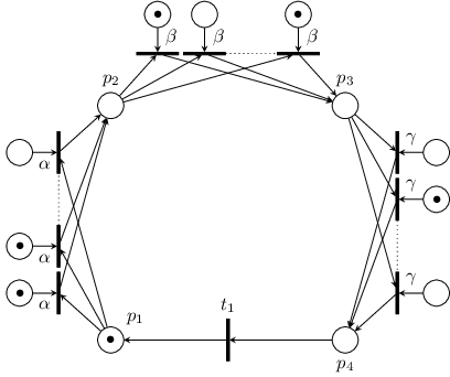
Suppose is a vertex cover for . We use the fact that if are two vertices not in that have the same set of neighbours, and have similar properties. This has been used to obtain Fpt algorithms for many hard problems (e.g. [9]). The following definitions formalize this.
Definition 6
Let be a vertex cover of . The (-) neighbourhood of a transition is the ordered pair . We denote by the number of different -neighbourhoods.
Definition 7
Suppose is a Petri net with neighbourhoods for vertex cover , and . The (-) interface of is defined as the function , where for every between and and every , there is a transition of VC-neighbourhood such that iff .
In the net in Fig. 9 with , all transitions labelled have the same VC-neighbourhood and all the corresponding places have the same VC-interface. Since there can be arcs between a transition and places in VC if , there can be at most different VC-neighbourhoods of transitions. There are at most VC-interfaces. The set of interfaces is denoted by .
Proposition 2
Let be a -safe net with being a vertex cover of . Let be places not in the vertex cover, all with the same interface. Let be some marking reachable from the initial marking of . If for some between and , then does not enable any transition that adds tokens to any of the places .
Proof
Suppose there is a transition enabled at that adds a token to for some between and . Then there is a transition with the same neighbourhood as (and hence enabled at too) that can add a token to . Firing from will create tokens at , contradicting the fact that is -safe. ∎
If the initial marking has tokens in many places with the same interface, then no transition can add tokens to any of those places until all the tokens in all those places are removed. Once all tokens are removed, one of the places can receive one token after which, no place can receive tokens until this one is removed. All these places have the same interface. Thus, a set of places with the same interface can be thought of as an initial storehouse of tokens, after depleting which it can be thought of as a single place. However, a formula in our logic can reason about individual places, so we still need to keep track of individual places that occur in the formula.
Proposition 3
Let be a -safe net and be an MSO formula. Let be the subset of places that occur in . Let and be two finite or infinite runs of such that for all positions of and for all , . For any assignment , we have iff .
Proof
By a straightforward induction on the structure of . ∎
Let be a -safe net such that has a vertex cover of size . Suppose is a formula and we have to check if satisfies . For each interface , let be the places not in with interface . If (i.e., if there are places in that are not in ), designate one of the places in as . Define the set of special places . Note that . Since this number is a function of the parameters of the input instance, we will treat it as a parameter.
We need a structure that keeps track of changes in places belonging to , avoiding a construction involving all reachable markings. This can be done by a finite state machine whose states are subsets of . Transitions of the Petri net that only affect places in can be simulated by the finite state machine with its usual transitions. To simulate transitions of the net that affect places outside , we need to impose some conditions on the number of times transitions of the finite state machine can be used. The following definition formalizes this. For a marking of , let .
Definition 8
Given a -safe net with initial marking and defined from as above, the edge constrained automaton is a structure defined as follows. and (recall that is the set of interfaces in ). The transition relation is such that for all and , iff there are markings and a transition of such that
- •
, and ,
- •
removes a token from a place of interface if and
- •
does not have any of its input or output places in if .
The edge constraint is given by . A subset is in iff for every marking with , the only transitions enabled at remove tokens from some place not in .
Intuitively, the edge constraint defines an upper bound on the number of times those transitions can be used that reduce tokens from places not in .
Definition 9
Let be an edge constrained automaton as in Def. 8 and let be a finite or infinite word over . Then is a valid run of iff for every position of , we can associate an element such that
- •
for every position of , and
- •
for every , .
- •
if is finite and is the last element of , then and for every interface and marking enabling some transition that removes tokens from some place in , .
Next we have a run construction lemma.
Lemma 4
Let be a -safe net with initial marking , be a formula and be as in Def. 8. For every infinite (maximal finite) run of , there exists an infinite (finite) run such that the word is a valid run of and for every position of , . If an infinite (finite) word over is a valid run of and , then there is an infinite (finite maximal) run of such that for all positions of .
Proof
Let be an infinite or a maximal finite run of . For every interface , perform the following steps: if for some marking in the above run, , let be the first such marking. By Prop. 2, no transition occurring before will add any token to any place in . If there is any transition occurring after that adds/removes tokens from , replace it with another transition with the same neighbourhood that adds/removes tokens from . By Prop. 2, such a replacement will not affect any place in and the new sequence of transitions is still enabled at . After performing this process for every interface , let the new run be . By construction, we have for all positions of . If is a maximal finite run, so is .
Now we will prove that the word is a valid run of . Suppose the sequence of transitions producing the run is . For each position of this run, define as follows:
- •
if has all its input and output places among places , let .
- •
if removes a token from some place in for some interface , let . Due to the way is constructed, this kind of transition can only occur before the position of and the number of such occurrences is at most .
Due to the way is constructed, there will not be any transition that adds tokens to any place in for any interface . By definition, it is clear that for every position of , . In addition, for every interface , we have . Hence, the word is a valid run of if the word is infinite. If is finite, suppose is the last marking of the sequence . Suppose for some variety , there is some marking such that and enables some transition that removes tokens from some place in . Since does not enable any transition, all transitions (including ) removing tokens from some place in are disabled in . This means that every place in that had a token in has lost its token in . Since such loss of tokens can only happen by firing transitions that remove tokens from places in , we have . Hence, to prove that is a valid run of , it is left to show that . To see that this is true, observe that if some marking with enables a transition that does not remove any token from , then so does , a contradiction.
Next, suppose is an infinite or finite word that is a valid run of such that . For every position of , there are , transition and markings and such that , , and . Define transitions as follows:
- •
If , transition has all its input and output places in . Let .
- •
If , transition removes a token from some place in . Let be a transition of the same neighbourhood as that removes a token from some place such that no transition among removes tokens from . This is possible since, due to the validity of in , . Let .
We will now prove by induction on that there are markings such that and for every position of .
Base case : If , the fact that , and that has all its input and output places in implies that for some such that . If , then removes a token from some place . Again the fact that and implies that for some such that .
Induction step: If , the fact that , and that has all its input and output places in implies that for some such that . If , then removes a token from some place . Again the fact that and implies that for some such that .
If is a finite word, we have to prove that the run constructed above is a maximal finite run. Let be the last marking in the sequence constructed above. We will prove that does not enable any transition. Suppose some transition is enabled at . Since , removes a token from some place in for some variety . Since , there are transition occurrences among that each remove a token from some place in . Since there were exactly places in that had a token in and no other transition adds any token to any place in , can not be enabled at . Hence, no transition is enabled at . ∎
Lemma 4 implies that in order to check if is a model of the formula , it is enough to check that all valid runs of satisfy . This can be done by checking that no finite valid run of is accepted by and no infinite valid run of is accepted by . As usual, this needs a product construction. Automata and run on the alphabet . Let and be the set of states of and respectively. Then, and .
Definition 10
, where
An accepting path of is a sequence which is -respecting:
- •
,
- •
the word witnesses the validity of the run in (as in Def. 9) and
- •
the word is accepted by through the run for some with .
An accepting path of is defined similarly.
Proposition 4
A -safe net with initial marking is a model of a formula iff there is no accepting path in and .
Proof
Suppose is a model of . Hence, all maximal runs of satisfy . We will prove that there is no accepting path in and . Assume by way of contradiction that there is an accepting path in . By Def. 10, is a valid run of . By Lemma 4, there is a finite maximal run of with for all positions . By Def. 10, is accepted by and hence satisfies . Proposition 3 now implies that satisfies , a contradiction. The argument for is similar.
Suppose is not a model of . Suppose there is a finite maximal run of that satisfies . By Lemma 4, there is a finite maximal run such that the word is a valid run of and for every position of , . By Prop. 3, satisfies and hence accepted by , say with the run . Let the word witness the validity of the run in , as in Def. 9. By Def. 10, the sequence is an accepting path of . The argument for maximal infinite runs is similar.∎
To efficiently check the existence of accepting paths in and , it is convenient to look at them as graphs, possibly with self loops and parallel edges. Let the set of states be the set of vertices of the graph and each transition be an -labelled edge leaving and entering . If there is a path in the graph from to , the number of times an edge occurs in is denoted by . If is some node occurring in , then the number of edges of entering is equal to the number of edges of leaving . These conditions can be expressed as integer linear constraints.
| (1) | ||||
Lemma 5 (Theorem 2.1, [20])
In a directed graph (possibly with self loops and parallel edges), let be a function such that the underlying undirected graph induced by edges such that is connected. Then, there is a path from to with each edge occurring times iff satisfies the constraints (1) above.
If the beginning and the end of a path are same (i.e., if ), small modifications of (1) and Lemma 5 are required. Finally we can prove our desired theorem.
Theorem 4.1
Let be a -safe net with initial marking and be a MSO formula. Parameterized by the vertex cover number of and the size of , checking whether is a model of is Fpt.
Proof
By Prop. 4, it is enough to check that there is no accepting paths in and . To check the existence of accepting paths in , we have to check if from some initial state in , we can reach some vertex in a maximal strongly connected component induced by -labelled edges, which contains some states from . For every such initial state and a vertex in such a strongly connected component, check the feasibility of (1) along with the following constraint for each interface :
| (2) |
To check the existence of accepting paths in , check the feasibility of (1) and (2) for every state in and every state in with some such that . If some marking with enables some transition removing a token from some place with interface , then for each such interface, add the following constraint:
| (3) |
The dependence of the running time of the above algorithm on formula size is non-elementary if the formula is MSO [15]. The dependence reduces to single exponential in case of LTL formulas [22]. The dependence on vertex cover number is dominated by the running time of Ilp, which is singly exponential in the number of its variables. The number of variables in turn depends on the number of VC-interfaces (Def. 7). In the worst case, this can be triply exponential but a given -safe Petri net need not have all possible VC-interfaces.
5 Conclusion
The main idea behind the Fpt upper bound for MSO/LTL model checking is the fact that the problem can be reduced to graph reachability and hence to Ilp. It remains to be seen if such techniques or others can be applied for branching time logics such as CTL.
We have some negative results with pathwidth and benefit depth as parameters and a positive result with vertex cover number as parameter. We think it is a challenging problem to identify other parameters associated with -safe Petri nets for which standard problems in the concurrency literature are Fpt. Another direction for further work, suggested by a referee, is to check if the upper bound can be extended to other classes of Petri nets such as communication-free nets.
The results of Sect. 3 proves hardness for the lowest level of the W-hierarchy. It remains to be seen if the lower bounds could be made tighter. The parameterized classes ParaNp and Xp include the whole W-hierarchy. Lower bounds or upper bounds corresponding to these classes would be interesting.
References
- [1] H. L. Bodlaender and T. Kloks. Efficient and constructive algorithms for the pathwidth and treewidth of graphs. J. Alg., 21(2):358–402, 1996.
- [2] J. R. Büchi. On a decision method in restricted second-order arithmetic. In Logic, Methodology, Philosophy and Science, pages 1–11. Stanford Univ Press, 1962.
- [3] B. Courcelle. The monadic second-order logic of graphs I: Recognizable sets of finite graphs. Information and Computation, 85:12–75, 1990.
- [4] S. Demri, F. Laroussinie, and P. Schnoebelen. A parametric analysis of the state-explosion problem in model checking. J. Comput. Syst. Sci., 72(4):547–575, 2006.
- [5] R. G. Downey and M. R. Fellows. Parameterized Complexity. Springer, 1999.
- [6] R. G. Downey, M. R. Fellows, and U. Stege. Parameterized complexity: A framework for systematically confronting computational intractability. In Contemporary Trends in Discrete Mathematics: From DIMACS and DIMATIA to the Future, volume 49 of DIMACS, pages 49–100. 1999.
- [7] D. Drusinsky and D. Harel. On the power of bounded concurrency I: Finite automata. J. Assoc. Comput. Mach., 41(3):517–539, 1994.
- [8] J. Esparza. Decidability and complexity of Petri net problems — An introduction, volume 1491 of LNCS, pages 374–428. 1998.
- [9] M. R. Fellows, D. Lokshtanov, N. Misra, F. A. Rosamond, and S. Saurabh. Graph layout problems parameterized by vertex cover. In ISAAC, volume 5369 of LNCS, pages 294–305, 2008.
- [10] J. Flum and M. Grohe. Describing parameterized complexity classes. Informatin and Computation, 187(2):291–319, 2003.
- [11] A. Frank and E. Tardos. An application of simultaneous diophantine approximation in combinatorial optimization. Combinatorica, 7(1):49–65, January 1987.
- [12] P. Habermehl. On the complexity of the linear-time -calculus for Petri-nets. In ATPN, volume 1248 of LNCS, pages 102–116, 1997.
- [13] R. Kannan. Minkowski’s convex body theorem and integer programming. Math. Oper. Res., 12(3):415–440, 1987.
- [14] H. W. Lenstra. Integer programming with a fixed number of variables. Math. Oper. Res., 8:538–548, 1983.
- [15] A. R. Meyer. Weak monadic second order theory of succesor is not elementary-recursive. In Proc. Logic Colloquium, volume 453 of Lecture Notes in Mathematics, pages 132–154. 1975.
- [16] M. Praveen. Does treewidth help in modal satisfiability? (extended abstract). In MFCS, volume 6281 of LNCS, pages 580–591, 2010. Full version http://arxiv.org/abs/1006.2461.
- [17] M. Praveen. Small vertex cover makes Petri net coverability and boundedness easier. In IPEC, volume 6478 of LNCS, pages 216–227, 2010.
- [18] M. Praveen and K. Lodaya. Modelchecking counting properties of 1-safe nets with buffers in parapspace. In FSTTCS, volume 4 of LIPIcs, pages 347–358, 2009.
- [19] C. Rackoff. The covering and boundedness problems for vector addition systems. Theoret. Comp. Sci., 6:223–231, 1978.
- [20] C. Reutenauer. The mathematics of Petri nets. 1990. Translated by I. Craig.
- [21] M. Samer and S. Szeider. Constraint satisfaction with bounded treewidth revisited. J. Comput. Syst. Sci., 76(2):103–114, 2010.
- [22] M. Vardi. An automata-theoretic approach to linear temporal logic. In F. Moller and G. Birtwistle, editors, Logics for Concurrency: Structure versus Automata, volume 1043 of LNCS, pages 238–266. 1996.