On the importance sampling of self-avoiding walks

Mireille Bousquet-Mélou Address: MBM: CNRS, LaBRI, Université Bordeaux 1, 351 cours de la Libération, 33405 Talence, France Email address: mireille.bousquet@labri.fr

Date: August 24th, 2012

Abstract.

In a 1976 paper published in Science, Knuth presented an algorithm to sample (non-uniform) self-avoiding walks crossing a square of side $k$ . From this sample, he constructed an estimator for the number of such walks. The quality of this estimator is directly related to the (relative) variance of a certain random variable $X_{k}$ . From his experiments, Knuth suspected that this variance was extremely large (so that the estimator would not be very efficient). But how large? For the analogous Rosenbluth algorithm, which samples unconfined self-avoiding walks of length $n$ , the variance of the corresponding estimator is believed to be exponential in $n$ .

A few years ago, Bassetti and Diaconis showed that, for a sampler à la Knuth that generates walks crossing a $k\times k$ square and consisting of North and East steps, the relative variance is only $O(\sqrt{k})$ . In this note we take one step further and show that, for walks consisting of North, South and East steps, the relative variance jumps to $2^{k(k+1)}/(k+1)^{2k}$ . This is quasi-exponential in the average length of the walks, which is of order $k^{2}$ . We also obtain partial results for general self-avoiding walks crossing a square, suggesting that the relative variance could be exponential in $k^{2}$ (which is again the average length of these walks).

Knuth’s algorithm is a basic example of a widely used technique called sequential importance sampling. The present paper, following Bassetti and Diaconis’ paper, is one of very few examples where the variance of the estimator can be found.

Key words and phrases:

Sampling – Self-avoiding walks

1. Introduction

A self-avoiding walk (SAW) on a graph is a walk that never visits the same vertex twice. Let $\mathcal{W}_{k}$ be the set of SAWs on a $k\times k$ square grid, going from the South-West vertex to the North-East vertex (Figure 2). In his paper “Coping with finiteness” [14, 15], Knuth described the following algorithm to generate a (non-uniform) random walk of $\mathcal{W}_{k}$ : start from the South-West corner, and at each time, choose with equal probability (which can be $1/3$ , $1/2$ or 1) one of the eligible steps. A step is eligible if, once appended to the current walk, it gives a self-avoiding walk that can be extended so as to end at the North-East corner. In this way the walk is never trapped and the algorithm always succeeds¹¹ 1 We describe in Section 5.3 how to detect algorithmically when a new step traps the walk.. Figure 1 shows the probabilities of the 12 possible walks when $k=2$ . Two bigger examples ( $k=10$ , $k=100$ ) are shown in Figure 2. This procedure is a basic example of a widely used technique called sequential importance sampling [5, 10, 11]. It is also a variant, for walks confined to a square, of the Rosenbluth algorithm that generates unconfined SAWs [21].

Refer to caption — Figure 1. The 12 self-avoiding walks crossing the $2\times 2$ square. For each of them, we give the sequence $1/p_{1},1/p_{2},\ldots$ where $p_{i}$ is the probability of the $i$ th step. The probability of the walk is thus the reciprocal of the product of the terms in the list. Two walks have probability $1/8$ , six have probability $1/12$ , and four have probability $1/16$ . Two walks that differ by a diagonal symmetry have the same probability.

Denote by $p(w)$ be the probability to draw the walk $w\in\mathcal{W}_{k}$ . Consider the random variable $X_{k}=1/p(w)$ , where $w$ is a random walk of $\mathcal{W}_{k}$ drawn according to the distribution $p(\cdot)$ . Clearly,

\mathbb{E}(X_{k})=\sum_{w\in\mathcal{W}_{k}}p(w)\frac{1}{p(w)}=|\mathcal{W}_{k}|.

Hence one can estimate the number of SAWs crossing a $k\times k$ square by generating $N$ walks $w^{(1)},\ldots,w^{(N)}$ of $\mathcal{W}_{k}$ , and computing

\frac{1}{N}\sum_{i=1}^{N}\frac{1}{p(w^{(i)})}.

(1)

By generating “several thousand” walks for $k=10$ , Knuth obtained

|\mathcal{W}_{10}|\simeq(1.6\pm 0.3)\times 10^{24},

which is quite good compared to the now known exact value, $1,568,758,030,464,750,013,214,100$ (see [7, 15]). We have reproduced Knuth’s experiment, and found, with a first group of 10,000 walks, the estimate $1.78\times 10^{24}$ , and with a second group, the estimate $1.38\times 10^{24}$ . As observed by Knuth, the values $\frac{1}{p(w^{(i)})}$ vary a lot (a small sample of 10 walks gave us values ranging from $10^{11}$ to $10^{24}$ ), and one may suspect that the variance of $X_{k}$ is probably much larger than $\mathbb{E}(X_{k})^{2}$ , or, in other words, that the relative variance

\Var\left(\frac{X_{k}}{\mathbb{E}(X_{k})}\right)

is large. Note that

\Var(X_{k})=\mathbb{E}(X_{k}^{2})-\mathbb{E}(X_{k})^{2}=\sum_{w\in\mathcal{W}_{k}}\frac{1}{p(w)}-|\mathcal{W}_{k}|^{2}.

Also, observe that the variance of the estimator (1) is $\Var(X_{k})/N$ , so that $\Var(X_{k})$ is a measure of the quality of this estimator. Let us mention that, even though sequential importance sampling is widely used, no general bounds on the variance of the estimators are available.

Knuth’s observation led Bassetti and Diaconis to study a simpler algorithm, in which a step, to be eligible, has to go North (N) or East (E) [5]. The resulting walk is called a directed walk, or NE-walk. Each step has probability $1/2$ unless it follows the North or East side of the square — in which case it has probability 1. Denote by $\mathcal{D}_{k}$ the set of directed walks of $\mathcal{W}_{k}$ , and by $p(w)$ the probability to generate the directed walk $w$ with this new algorithm. Define the random variable $X_{k}=1/p(w)$ as above. Then

\mathbb{E}(X_{k})=|\mathcal{D}_{k}|={2k\choose k}\sim\frac{4^{k}}{\sqrt{\pi k}}.

Of course, since $|\mathcal{D}_{k}|$ is known exactly, there is no point in using importance sampling to estimate this cardinality — but it is interesting to know that the variance of the estimator can be determined, as follows. By the above argument, a walk of $\mathcal{D}_{k}$ that hits the North or East side of the square for the first time at time $k+i$ has probability $1/2^{k+i}$ . Since there are $2{k+i-1\choose i}$ such walks,

\mathbb{E}(X_{k}^{2})=\sum_{w\in\mathcal{D}_{k}}\frac{1}{p(w)}=\sum_{i=0}^{k-1}2^{k+i+1}{k+i-1\choose i}.

The corresponding generating function is

\sum_{k\geq 1}\mathbb{E}(X_{k}^{2})x^{k}=\frac{2\,x}{1+2x}\left({\frac{3}{\sqrt{1-16\,x}}}-1\right),

(2)

and an elementary singularity analysis [12, Chap. VI] gives

\mathbb{E}(X_{k}^{2})\sim\frac{16^{k}}{3\sqrt{\pi k}},

which is roughly $\sqrt{k}$ times larger than

\mathbb{E}(X_{k})^{2}\sim\frac{16^{k}}{{\pi k}}.

In this note, we first take one more step in the direction of the general problem by declaring that South steps are also eligible. The resulting walks are partially directed walks, or NES-walks. The probabilities of the 9 walks obtained when $k=2$ are shown in Figure 3. Of course, these probabilities are not the same as those obtained from Knuth’s original algorithm.

Figure 3. The nine NES-walks crossing a

2\times 2

square, with the reciprocals of the probabilities of their steps.

We will prove that one outcome of this increased generality is that the ratio between $\mathbb{E}(X_{k}^{2})$ and $\mathbb{E}(X_{k})^{2}$ becomes much larger:

\mathbb{E}(X_{k}^{2})\sim\frac{3}{2}\,2^{k(k+1)}\quad\hbox{while}\quad\mathbb{E}(X_{k})^{2}=(k+1)^{2k}.

We will also prove that the average length of a (uniform) NES-walk confined to the $k\times k$ square is quadratic in $k$ , so that the variance of $X_{k}$ is roughly exponential in the length, as predicted for SAWs generated by the Rosenbluth algorithm [6].

Since the $x/y$ symmetry is lost with partially directed walks, it is natural to generalize the original question by enclosing walks in a rectangle $R$ of height $k$ and width $\ell$ . Thus, let $\mathcal{P}_{k,\ell}$ be the set of partially directed walks that start from the South-West corner of $R$ and end at the North-East corner. A walk of $\mathcal{P}_{k,\ell}$ contains exactly $\ell$ East steps, and choosing the heights of these steps determines the walk completely. Hence the number of walks in $\mathcal{P}_{k,\ell}$ is $(k+1)^{\ell}$ .

Thus, defining the random variable $X_{k,\ell}=1/p(w)$ as above, we have

\mathbb{E}(X_{k,\ell})=|\mathcal{P}_{k,\ell}|=(k+1)^{\ell}.

(3)

We will prove that, if $k,\ell\rightarrow\infty$ in such a way $\ell=o(2^{k})$ , then

\Var(X_{k,\ell})\sim\mathbb{E}(X_{k,\ell}^{2})\sim\frac{3}{2}\,2^{(k+1)\ell},

so that the relative variance satisfies

\Var\left(\frac{X_{k,\ell}}{\mathbb{E}(X_{k,\ell})}\right)\sim\frac{3}{2}\,\left(\frac{2^{k+1}}{(k+1)^{2}}\right)^{\ell}.

This results thus extends the very short list of examples where the variance of an importance sampler can be rigorously established [5]. Moreover, the average length of a (uniform) walk of $\mathcal{P}_{k,\ell}$ is shown to be approximately $k\ell/3$ , so that the variance is again exponential in the length, as expected for other similar samplers.

The paper is organized as follows. In Section 2, we obtain an explicit expression for the generating function of the numbers $\mathbb{E}(X_{k,\ell}^{2})$ (the counterpart of (2)). In Section 3, we derive from this expression the above asymptotic result. In Section 4, we go back to Knuth’s sampler and prove that there exist two positive constants $\lambda$ and $\beta$ such that

\mathbb{E}(X_{k})^{1/k^{2}}\rightarrow\lambda\quad\hbox{and}\quad\mathbb{E}(X_{k}^{2})^{1/k^{2}}\rightarrow\beta.

The former result has actually been known since 1978 [1]. Since a variance is non-negative, $\beta\geq\lambda^{2}$ . Upper (and lower) bounds on $\lambda$ have been obtained in [7], based on the determination of the numbers $\mathbb{E}(X_{k})=|\mathcal{W}_{k}|$ for small values of $k$ , and of related numbers counting other configurations of self-avoiding walks. As shown in Section 4, a similar study, performed for the numbers $\mathbb{E}(X_{k}^{2})$ , might suffice to prove that $\beta>\lambda^{2}$ , so that the variance would be again exponential in $k^{2}$ (which is known to be the average length of a uniform SAW crossing the $k\times k$ -square [16]). We conclude with a few remarks and questions on the importance sampling of self-avoiding walks not confined to a box.

2. Exact results for NES-walks

In this section, we first describe the probability $p(w)$ to obtain the walk $w$ in terms of the geometry of $w$ (Section 2.1). This description reduces the determination of the numbers $\mathbb{E}(X_{k,\ell}^{2})$ to the enumeration of NES-walks according to several parameters, which we perform in Section 2.2.

2.1. The probability $p(w)$

Let $w_{0}$ be a walk of $\mathcal{P}_{k,\ell}$ , written as a sequence of N, E and S steps. Let $w$ be the prefix of $w_{0}$ that precedes the last E step. That is, $w_{0}=w{\sf E}{\sf N}\cdots{\sf N}$ . By convention, $w_{0}$ starts at height 0.

Lemma 1.

The probability $p(w_{0})$ to obtain $w_{0}$ via the importance sampling algorithm satisfies

\frac{1}{p(w_{0})}=2\cdot 3^{h(w)}2^{h_{c}(w)}2^{v(w)}1^{v_{c}(w)},

where

•

$h(w)$ is the number of horizontal steps of $w$ that lie neither at height $0$ nor at height $k$ ,
•

$h_{c}(w)$ is the number of horizontal contacts of $w$ , that is, horizontal steps that lie at height $0$ or $k$ ,
•

$v(w)$ is the number of vertical steps of $w$ that end neither at height $0$ nor at height $k$ ,
•

$v_{c}(w)$ is the number of vertical contacts of $w$ , that is, vertical steps that end at height $0$ or $k$ .

Proof.

Assume the walk $w_{0}$ has length $n$ and ends with exactly $j$ vertical steps. The probability of the first step is $1/2$ , and the probability of each of the $j$ final steps is 1. Let $s_{i}$ denote the $i$ th step. Hence $w$ consists of the steps $s_{1},\ldots,s_{n-j-1}$ . For $1\leq i<n-j$ , the probability of $s_{i+1}$ depends on the direction and position of $s_{i}$ :

•

if $s_{i}$ is horizontal, but not a contact, then the probability of $s_{i+1}$ is $1/3$ ,
•

if $s_{i}$ is a horizontal contact, then the probability of $s_{i+1}$ is $1/2$ ,
•

if $s_{i}$ is vertical, but not a contact, then the probability of $s_{i+1}$ is $1/2$ ,
•

if $s_{i}$ is a vertical contact, then the probability of $s_{i+1}$ is $1$ .

The lemma follows.

2.2. Enumeration of NES-walks in a strip of fixed height

Recall the expression (3) of the numbers $\mathbb{E}(X_{k,\ell})$ . For $k$ (the height of the rectangle) fixed, the generating function of the numbers $\mathbb{E}(X_{k,\ell})^{2}$ is rational:

\sum_{\ell\geq 1}\mathbb{E}(X_{k,\ell})^{2}x^{\ell}=\sum_{\ell\geq 1}(k+1)^{2\ell}x^{\ell}=\frac{(k+1)^{2}x}{1-(k+1)^{2}x}.

(4)

We will determine the variance of $X_{k,\ell}$ by describing the generating function of the numbers $\mathbb{E}(X_{k,\ell}^{2})$ , which is also rational when $k$ is fixed.

Proposition 2.

For any fixed height $k$ , the generating function $M_{k}(x)$ of the numbers $\mathbb{E}(X_{k,\ell}^{2})$ is a rational series:

M_{k}(x):=\sum_{\ell\geq 1}\mathbb{E}(X_{k,\ell}^{2})x^{\ell}=2x\,\frac{N_{k}}{G_{k}},

where $N_{k}$ and $G_{k}$ are polynomials in $x$ satisfying the same recurrence relation:

N_{k}=(5+9x)N_{k-2}-4N_{k-4},

(and similarly for $G_{k}$ ), with initial conditions

\begin{array}[]{lllllllll}N_{1}&=&2,&&G_{1}&=&1-4x,\\ N_{2}&=&5+3x,&&G_{2}&=&1-9x-6x^{2},\\ N_{3}&=&11+9x,&&G_{3}&=&1-19x-18x^{2},\\ N_{4}&=&23+54x+27x^{2},&&G_{4}&=&1-36x-99x^{2}-54x^{3}.\end{array}

Example. For $k=2$ ,

\sum_{\ell\geq 1}\mathbb{E}(X_{2,\ell}^{2})x^{\ell}=2x\,\frac{5+3x}{1-9x-6x^{2}}=10x+96x^{2}+O(x^{3}).

Figure 3 allows us to check that the coefficient of $x^{2}$ is correct:

96=4+8+8+12+12+8+12+16+16.

The generating function of the variances is

\sum_{\ell\geq 1}\Var(X_{2,\ell})x^{\ell}=2x\,\frac{5+3x}{1-9x-6x^{2}}-\frac{9x}{1-9x}.

Observe that the radius of the first fraction is smaller than the radius of the second fraction. As $\ell\rightarrow\infty$ ,

\mathbb{E}(X_{2,\ell}^{2})\sim\mu^{\ell}

(up to a multiplicative constant) with $\mu=(9+\sqrt{105})/2\simeq 9.62$ , while $\mathbb{E}(X_{2,\ell})^{2}=9^{\ell}$ .

We now want to prove Proposition 2. Recall that

\mathbb{E}(X_{k,\ell}^{2})=\sum_{w_{0}\in\mathcal{P}_{k,\ell}}\frac{1}{p(w_{0})}.

The expression of $p(w_{0})$ given in Lemma 1 leads us to study a purely enumerative problem. For $k$ fixed, let $\mathcal{T}_{k}$ be the set of NES-walks $w$ that start at height $0$ and are confined to the strip $0\leq y\leq k$ . We wish to count these walks by the parameters $h(w)$ , $h_{c}(w)$ , $v(w)$ and $v_{c}(w)$ . So, let

\sum_{w\in\mathcal{T}_{k}}x^{h(w)}y^{v(w)}a^{h_{c}(w)}b^{v_{c}(w)}

be the associated generating function. This series is easily seen to be rational (it can be determined using a transfer-matrix approach [22, Sec. 4.7], or equivalently a finite-state automaton [12, p. 362]), and there are several ways to determine it. We present here what we believe to be the most direct one. It relies on a recursive description of the walks of $\mathcal{T}_{k}$ , where we add at each time an E step and a sequence of vertical steps. This approach requires to take into account an additional parameter, namely the height $f(w)$ of the final point of the walk $w$ . Hence our series finally involve 5 variables:

T_{k}(s)\equiv T_{k}(x,y,a,b;s)=\sum_{w\in\mathcal{T}_{k}}x^{h(w)}y^{v(w)}a^{h_{c}(w)}b^{v_{c}(w)}s^{f(w)}.

We will denote by $\tilde{\mathcal{T}}_{k}$ the subset of $\mathcal{T}_{k}$ formed of walks that do not end at height 0 or $k$ , and by $\tilde{T}_{k}(s)\equiv\tilde{T}_{k}(x,y,a,b;s)$ the corresponding generating function. Accordingly,

T_{k}(s)=\sum_{i=0}^{k}T_{k,i}s^{i}=T_{k,0}+\tilde{T}_{k}(s)+s^{k}T_{k,k},

where $T_{k,i}$ is the series in $x$ , $y$ , $a$ and $b$ counting walks of $\mathcal{T}_{k}$ ending at height $i$ . By Lemma 1,

$\displaystyle M_{k}(x)=\sum_{\ell\geq 1}\mathbb{E}(X_{k,\ell}^{2})x^{\ell}$	$\displaystyle=$	$\displaystyle\sum_{\ell\geq 1}\sum_{w_{0}\in\mathcal{P}_{k,\ell}}\frac{1}{p(w_{0})}x^{\ell}$	(5)
	$\displaystyle=$	$\displaystyle 2\sum_{w\in\mathcal{T}_{k}}3^{h(w)}2^{h_{c}(w)}2^{v(w)}x^{1+h(w)+h_{c}(w)}$
	$\displaystyle=$	$\displaystyle 2x\,T_{k}(3x,2,2x,1;1).$

Remark. The series $T_{k,k}$ has already been determined in the case $x=y=a=b=t$ , using the same approach as here [3, Prop 3]. The derivation is more involved here because we keep track of four parameters in the enumeration, and because we are interested in $T_{k}(1)$ rather than $T_{k,k}$ .

Lemma 3.

The series $\tilde{T}_{k}(s)$ , $T_{k,0}$ and $T_{k,k}$ satisfy the following system of equations:

\left(1-\frac{x}{1-ys}-\frac{xy\bar{s}}{1-y\bar{s}}\right)\tilde{T}_{k}(s)\\ =\frac{ys-(ys)^{k}}{1-ys}-\frac{x(ys)^{k}}{1-ys}\tilde{T}_{k}(1/y)-\frac{x}{1-y\bar{s}}\tilde{T}_{k}(y)+aT_{k,0}\frac{ys-(ys)^{k}}{1-ys}+aT_{k,k}\frac{ys^{k-1}-y^{k}}{1-y\bar{s}},

	$\displaystyle T_{k,0}$	$\displaystyle=$	$\displaystyle 1+bx\bar{y}\tilde{T}_{k}(y)+aT_{k,0}+aby^{k-1}T_{k,k},$
	$\displaystyle T_{k,k}$	$\displaystyle=$	$\displaystyle by^{k-1}+bxy^{k-1}\tilde{T}_{k}(1/y)+aby^{k-1}T_{k,0}+aT_{k,k},$

with $\bar{s}=1/s$ and $\bar{y}=1/y$ .

Proof.

We construct the walks of $\tilde{\mathcal{T}}_{k}$ recursively, by adding at each time a horizontal step followed by a sequence of vertical steps.

We partition the set $\tilde{\mathcal{T}}_{k}$ into three disjoint subsets, illustrated in Figure 4.

•

The first subset consists of walks with no E step. These walks consist of $i$ North steps, with $1\leq i<k$ . Their generating function is

$\sum_{i=1}^{k-1}(ys)^{i}=\frac{ys-(ys)^{k}}{1-ys}.$

•

The second subset consists of walks in which the last E is followed by a (possibly empty) sequence of N steps. We denote by $i$ the height of the last E step, and distinguish the cases $i=0$ and $0<i<k$ . The generating function of this subset of $\tilde{\mathcal{T}}_{k}$ reads

	$\displaystyle aT_{k,0}\sum_{j=1}^{k-1}(sy)^{j}+x\sum_{i=1}^{k-1}\left(T_{k,i}s^{i}\sum_{j=0}^{k-i-1}(ys)^{j}\right)=aT_{k,0}\frac{ys-(ys)^{k}}{1-ys}+x\sum_{i=1}^{k-1}\left(T_{k,i}s^{i}\frac{1-(ys)^{k-i}}{1-ys}\right)$
	$\displaystyle=aT_{k,0}\frac{ys-(ys)^{k}}{1-ys}+\frac{x}{1-ys}\left(\tilde{T}_{k}(s)-(ys)^{k}\tilde{T}_{k}(1/y)\right).$

•

The third subset consists of walks in which the last E step is followed by a non-empty sequence of S steps. We denote by $i$ the height of the last E step, and distinguish the cases $i=k$ and $0<i<k$ . The generating function of this subset of $\tilde{\mathcal{T}}_{k}$ reads

	$\displaystyle as^{k}T_{k,k}\sum_{j=1}^{k-1}(y\bar{s})^{j}+x\sum_{i=1}^{k-1}\left(T_{k,i}s^{i}\sum_{j=1}^{i-1}(y\bar{s})^{j}\right)=aT_{k,k}\frac{ys^{k-1}-y^{k}}{1-y\bar{s}}+x\sum_{i=1}^{k-1}\left(T_{k,i}s^{i}\frac{y\bar{s}-(y\bar{s})^{i}}{1-y\bar{s}}\right)$
	$\displaystyle=aT_{k,k}\frac{ys^{k-1}-y^{k}}{1-y\bar{s}}+\frac{x}{1-y\bar{s}}\left(y\bar{s}\tilde{T}_{k}(s)-\tilde{T}_{k}(y)\right).$

Adding the three contributions gives the series $\tilde{T}_{k}(s)$ and establishes the first equation of the lemma.

The equations for $T_{k,0}$ and $T_{k,k}$ are obtained in a similar fashion.

Figure 4. Recursive construction of bounded NES-walks.

We now solve the functional equations of Lemma 3. The key tool is the kernel method (see e.g. [4, 8, 20]).

Proposition 4.

Let $k\geq 1$ . The series $T_{k}(1)\equiv T_{k}(x,y,a,b;1)$ counting NES-walks confined to a strip of height $k$ is

T_{k}(1)=\frac{N_{k}}{G_{k}},

where $N_{k}$ and $G_{k}$ are polynomials in $x$ , $y$ , $a$ and $b$ satisfying the same recurrence relation

N_{k}=(1-x+y^{2}(1+x))N_{k-2}-y^{2}N_{k-4},

(and similarly for $G_{k}$ ) with initial conditions

\begin{array}[]{llllllll}N_{-1}&=&(1-x-xy)(b-y)/y^{2},&&G_{0}&=&(x-1)ab/y-(x+1)(a-1),\\ N_{0}&=&(b-xb+xy)/y,&&G_{1}&=&1-a-ab,\\ N_{1}&=&1+b,&&G_{2}&=&(1-x)(1-a)-(x+1)yab,\\ N_{2}&=&1-x+y+by(1+x),&&G_{3}&=&(1-x-xy)(1-a)-yab(x+y+xy).\end{array}

Equivalently,

T_{k}(1)=\frac{1}{P(\bar{S})S^{k}+P(S)}\left(Q(\bar{S})S^{k}+Q(S)+(1-y^{2})\frac{S^{k}-S}{S-1}\right),

(6)

where $S$ is the unique formal power series²² 2 The other solution is $1/S$ , and its expansion in $x$ and $y$ involves negative powers of $y$ . in $x$ and $y$ satisfying

S+\frac{1}{S}=(1+x)y+(1-x)\bar{y},

(7)

with $\bar{y}=1/y$ , $\bar{S}=1/S$ ,

P(s)=1-a+aby-s(ab+y-ay)\quad\hbox{and }\quad Q(s)=1-by+(b-y)s.

(8)

The reason why we give the expressions of $N_{-1}$ and $N_{0}$ , rather than $N_{3}$ and $N_{4}$ , is that they are more compact. The same reason explains why we give $G_{0}$ rather than $G_{4}$ . It is of course easy to compute $N_{3}$ , $N_{4}$ and $G_{4}$ , and Proposition 2 then follows at once, using (5). We hope that using the same notation $N_{k}$ , $G_{k}$ , for the enumeration problem of Proposition 4 and its specialization of Proposition 2 will not create any confusion.

Proof.

First, we use the last two equations of Lemma 3 to express $\tilde{T}_{k}(y)$ and $\tilde{T}_{k}(1/y)$ as linear combinations of $T_{k,0}$ and $T_{k,k}$ . Then, in the first equation of the lemma, we replace $\tilde{T}_{k}(y)$ and $\tilde{T}_{k}(1/y)$ by their expressions in terms of $T_{k,0}$ and $T_{k,k}$ . The left-hand side is unchanged, and the right-hand side now involves only two unknown series, namely $T_{k,0}$ and $T_{k,k}$ :

\left(1-{\frac{x}{1-ys}-{\frac{xy\bar{s}}{1-y\bar{s}}}}\right)\tilde{T}_{k}(s)\\ =\frac{ys}{1-ys}+\frac{y}{b\left(1-y\bar{s}\right)}+\left({\frac{ays}{1-ys}}+{\frac{y\left(a-1\right)}{b\left(1-y\bar{s}\right)}}\right)T_{k,0}+{s}^{k}\left({\frac{y\left(a-1\right)}{b\left(1-ys\right)}}+{\frac{ya\bar{s}}{1-y\bar{s}}}\right)T_{k,k}.

(9)

The kernel of this equation is the coefficient of $\tilde{T}_{k}(s)$ . It vanishes when $s=S$ and $s=\bar{S}:=1/S$ , where $S$ is defined in the proposition. Since $\tilde{T}_{k}(s)$ is a polynomial in $s$ , and $S$ and $\bar{S}$ are Laurent series in $x$ and $y$ with finitely many monomials with negative exponents, the series $\tilde{T}_{k}(S)$ and $\tilde{T}_{k}(\bar{S})$ are well-defined. Replacing $s$ by $S$ or $\bar{S}$ in the above equation cancels the left-hand side, and hence the right-hand side. One thus obtains two linear equations between $T_{k,0}$ and $T_{k,k}$ , which involve the series $S$ . Solving them gives expressions of $T_{k,0}$ and $T_{k,k}$ in terms of $S$ (the expression of $T_{k,k}$ is given in (11) below). By setting $s=1$ in (9), one then expresses $\tilde{T}_{k}(1)$ in terms of $S$ , and finally $T_{k}(1)=T_{k,0}+T_{k,k}+\tilde{T}_{k}(1)$ . This gives (6).

Observe that the expression (6) is unchanged if we replace $S$ by $\bar{S}=1/S$ . In particular, it can be written as a symmetric rational function in $S$ and $\bar{S}$ (with coefficients in ${\mathbb{Q}}(a,b,y)$ ). Since $S$ and $\bar{S}$ are the two roots of (7), their symmetric functions are rational functions of $x$ and $y$ . This implies that $T_{k}(1)$ is a rational series in $x$ , $y$ , $a$ and $b$ . However, the denominator of (6), namely $P(\bar{S})S^{k}+P(S)$ , is not unchanged when $S\mapsto 1/S$ . But let us define the series $N_{k}$ and $G_{k}$ as follows:

$\displaystyle G_{2k}$	$\displaystyle=$	$\displaystyle\frac{y^{k}}{1-y^{2}}\left(P(\bar{S})S^{k}+P(S)\bar{S}^{k}\right),$
$\displaystyle G_{2k+1}$	$\displaystyle=$	$\displaystyle\frac{y^{k}}{(1-y)(1+S)}\left(P(\bar{S})S^{k+1}+P(S)\bar{S}^{k}\right),$	(10)
$\displaystyle N_{2k}$	$\displaystyle=$	$\displaystyle\frac{y^{k}}{1-y^{2}}\left(Q(\bar{S})S^{k}+Q(S)\bar{S}^{k}+(1-y^{2})\frac{S^{k}-\bar{S}^{k-1}}{S-1}\right),$
$\displaystyle N_{2k+1}$	$\displaystyle=$	$\displaystyle\frac{y^{k}}{(1-y)(1+S)}\left(Q(\bar{S})S^{k+1}+Q(S)\bar{S}^{k}+(1-y^{2})\frac{S^{k}-\bar{S}^{k}}{1-\bar{S}}\right).$

Then it is easy to check that (6) can be rewritten as $T_{k}(1)=N_{k}/G_{k}$ . Moreover, the series $N_{k}$ and $G_{k}$ are unchanged when $S\mapsto 1/S$ , and hence, by the same argument as above, they are rational functions of $x$ , $y$ , $a$ and $b$ . More precisely, each of the sequences $G_{2k}$ , $G_{2k+1}$ , $N_{2k}$ and $N_{2k+1}$ is of the form $y^{k}(\alpha S^{k}+\beta\bar{S}^{k})$ , where $S$ and $\bar{S}$ are the two roots of (7). Hence each sequence satisfies the recurrence relation

u_{k}=(1-x+y^{2}(1+x))u_{k-1}-y^{2}u_{k-2}.

One easily determines the initial values for each sequence. This yields the description of $N_{k}$ and $G_{k}$ given in the proposition. From this description, it is clear that $N_{k}$ and $G_{k}$ are polynomials, as soon as $k\geq 1$ .

Remarks
1. Denominators. The series $T_{k,i}$ , counting walks ending at height $i$ , are also rational, but with a denominator that is a proper multiple of the denominator of $T_{k}(1)=\sum_{i=0}^{k}T_{k,i}$ . For instance,

T_{k,k}=\frac{b(y^{2}-1)(\bar{S}-S)S^{k}}{(P(\bar{S})S^{k}-P(S))(P(\bar{S})S^{k}+P(S))},

(11)

or, in terms of polynomials,

T_{k,k}=\frac{by^{k-1}}{F_{k}},

(12)

where $F_{k}$ is defined by the recurrence relation

F_{k}=(1-x+(1+x)y^{2})F_{k-1}-y^{2}F_{k-2},

with the initial conditions

F_{1}=(1-a-ab)(1-a+ab)\quad\hbox{and}\quad F_{2}=(1-a+bya)((1-x)(1-a)-(x+1)yab).

It is not hard to prove that $G_{k}$ , the denominator of $T_{k}(1)$ , is a divisor of $F_{k}$ . The simplification that occurs in the denominator when summing the series $T_{k,i}$ over $i$ has recently been explained combinatorially, for slightly different walk models, by Bacher [2].

2. Average length. The series $T_{k,k}(tx,t,tx,t)$ counts NES-walks crossing a strip of height $k$ according to the length (variable $t$ ) and the width (variable $x$ ). In particular, the case $t=1$ of (12) reads $T_{k,k}(x,1,x,1)=1/(1-(k+1)x)$ , as justified combinatorially in the introduction. In order to determine the average length $|w|$ of a uniform NES-walk $w$ crossing a $k\times\ell$ rectangle, we differentiate $T_{k,k}(tx,t,tx,t)$ with respect to $t$ , and then set $t=1$ . This gives

\left.\frac{\partial}{\partial t}\left(T_{k,k}(tx,t,tx,t)\right)\right|_{t=1}=\sum_{\ell\geq 0}x^{\ell}\sum_{w\in\mathcal{P}_{k,\ell}}|w|={\frac{k}{1-x\left(1+k\right)}}+{\frac{x\left(1+k\right)\left(1+k\left(k+2\right)x/3\right)}{\left(1-x\left(1+k\right)\right)^{2}}},

so that the average length is

{\frac{\left({k}^{2}+5\,k+3\right)\ell}{3(1+k)}}+{\frac{k\left(2\,k+1\right)}{3(1+k)}}=\frac{k\ell}{3}+O(k+\ell).

(13)

3. Asymptotic results for NES-walks

We now derive asymptotic results from the previous section. Recall that $\mathbb{E}(X_{k,\ell})=(k+1)^{\ell}$ , so that the generating function of the numbers $\mathbb{E}(X_{k,\ell})^{2}$ is given by (4) (for $k$ fixed), with radius of convergence $1/(k+1)^{2}$ . The radius of convergence of the generating function of the numbers $\mathbb{E}(X_{k,\ell}^{2})$ turns out to be exponentially smaller. Our study has analogies with the study of the longest run in a binary string [12, p. 308], which also requires to analyze (explicit) rational functions depending on an integer $k$ .

Proposition 5.

Let $k\geq 1$ . The series $M_{k}(x)$ , given in Proposition 2, has a unique pole $\rho_{k}$ of modulus less than $1/9$ , satisfying

\rho_{k}=\frac{1}{2^{k+1}}+\frac{9}{2\cdot 4^{k+1}}-\frac{12k-23}{2\cdot 8^{k+1}}+\frac{36k^{2}-54k-87/8}{16^{k+1}}+O\left(\frac{k^{3}}{32^{k}}\right).

(14)

As $x\rightarrow\rho_{k}^{-}$ ,

M_{k}(x)\sim\frac{\alpha_{k}}{1-x/\rho_{k}}

(15)

with

\alpha_{k}=\frac{3}{2}-\frac{9k-4}{2^{k+2}}+\frac{27k^{2}-48k+1}{2\cdot 4^{k+1}}-\frac{81k^{3}-306k^{2}+75k+140}{2\cdot 8^{k+1}}+O\left(\frac{k^{4}}{16^{k}}\right).

(16)

The second moment of $X_{k,\ell}$ satisfies, uniformly in $k$ and $\ell$ ,

\mathbb{E}(X_{k,\ell}^{2})=\alpha_{k}\rho_{k}^{-\ell}+O(9^{\ell}k).

In particular, if $k,\ell\rightarrow\infty$ in such a way $\ell=o(2^{k})$ , then

\Var(X_{k,\ell})\sim\mathbb{E}(X_{k,\ell}^{2})\sim\frac{3}{2}\,2^{(k+1)\ell},

which is much larger than $\mathbb{E}(X_{k,\ell})^{2}=(k+1)^{2\ell}$ . By (13), the variance is thus exponential in the average length of a (uniform) NES-walk crossing the $k\times\ell$ rectangle.

Proof.

We proceed in four steps. We first express the series $M_{k}(x)$ in terms of an algebraic series $S$ , as was done for the enumerative problem in Proposition 4. Then, we study the analytic properties of $S$ . We use these properties to prove that the denominator $G_{k}$ of $M_{k}$ is real-rooted, with one positive zero $\rho_{k}$ and all the other zeroes below $-1/9$ . We finally apply Cauchy’s formula to extract the $\ell$ th coefficient of $M_{k}(x)$ , which is $\mathbb{E}(X_{k,\ell}^{2})$ .

Step 1. The expression of $M_{k}$
By Proposition 2,

M_{k}(x)=2x\frac{N_{k}}{G_{k}},

where the polynomials $N_{k}$ and $G_{k}$ can be described either by induction, or, after performing the change of variables $x\rightarrow 3x$ , $a\rightarrow 2x$ , $y\rightarrow 2$ and $b\rightarrow 1$ in (10), by³³ 3 From now on, we carefully avoid the notation $\bar{S}:=1/S$ , since we will soon be doing complex analysis.

$\displaystyle G_{2k}$	$\displaystyle=$	$\displaystyle-\frac{2^{k}}{3}\left(P(1/S)S^{k}+P(S)S^{-k}\right),$
$\displaystyle G_{2k+1}$	$\displaystyle=$	$\displaystyle-\frac{2^{k}}{1+S}\left(P(1/S)S^{k+1}+P(S)S^{-k}\right),$	(17)
$\displaystyle N_{2k}$	$\displaystyle=$	$\displaystyle-\frac{2^{k}}{3}\left(Q(1/S)S^{k}+Q(S)S^{-k}-3\frac{S^{k}-S^{-k+1}}{S-1}\right),$
$\displaystyle N_{2k+1}$	$\displaystyle=$	$\displaystyle-\frac{2^{k}}{1+S}\left(Q(1/S)S^{k+1}+Q(S)S^{-k}-3\frac{S^{k}-S^{-k}}{1-1/S}\right),$

where $S$ and $1/S$ are the two power series in $x$ satisfying

S+\frac{1}{S}=\frac{5+9x}{2},

(18)

or equivalently,

x=-\frac{1}{9}(2S-1)\left(2/S-1\right).

(19)

The polynomials $P(s)$ and $Q(s)$ are

P(s)=1+2x-2s(1-x)\quad\hbox{and}\quad Q(s)=-1-s,

so that, in view of (19),

P(S)=\frac{(2S-1)(2S^{2}-11S-4)}{9S}\quad\hbox{and}\quad P(1/S)=\frac{(2-S)(2-11S-4S^{2})}{9S^{2}}.

It also follows from (5) and (6) that

M_{k}(x)=\frac{2x}{P(\bar{S})S^{k}+P(S)}\left(Q(\bar{S})S^{k}+Q(S)-3\,\frac{S^{k}-S}{S-1}\right).

(20)

Step 2. The series $S(x)$
From now on, we denote by $S$ the root of (18) that has constant term 1/2:

S=\frac{5+9x-3\sqrt{(1+x)(1+9x)}}{4}.

(21)

Lemma 6.

The series $S$ has radius of convergence $1/9$ , and admits an analytic continuation, still denoted by $S$ , in ${\mathbb{C}}\setminus[-1,-1/9]$ . In this domain, $S$ never vanishes, and its modulus is less than $1$ .

Proof.

The existence of an analytic continuation follows from basic complex analysis. If $x=u+iv$ , the imaginary part of the discriminant $(1+x)(1+9x)$ reads $2v(5+9u)$ . Using the principal determination of the square root, the analytic continuation of $S$ is given by (21) when $\Re(x)\geq-5/9$ , and otherwise by

S=\frac{5+9x+3\sqrt{(1+x)(1+9x)}}{4}.

A plot of the modulus of $S$ is shown in Figure 5 (left).

Step 3. The roots of $G_{k}$

Lemma 7.

For $k\geq 1$ , the denominator $G_{k}$ of the series $M_{k}$ is real-rooted. It has a unique positive zero $\rho_{k}$ , which, as $k\rightarrow\infty$ , admits the expansion (14). The other zeroes are smaller than $-1/9$ . As $x$ approaches $\rho_{k}$ , the series $M_{k}$ behaves likes $\alpha_{k}/(1-x/\rho_{k})$ , where $\alpha_{k}$ admits the expansion (16).

We could use Rouché’s theorem to prove that, for any $\varepsilon>0$ , the polynomial $G_{k}$ has only one root of modulus less than $1/9-\varepsilon$ for $k$ large enough, but the above statement is more precise.

Proof.

The case $k=1$ being trivial ( $G_{1}=1-4x$ ), we focus on the case $k\geq 2$ . By Proposition 2, the denominator $G_{k}$ has degree $\lceil\frac{k+1}{2}\rceil$ . The expressions (17) are symmetric in $S$ and $1/S$ , and thus hold for any determination of $S$ , and thus for any $x\in{\mathbb{C}}$ , including in the cut $[-1,-1/9]$ . They show that $G_{k}(x)=0$ if and only if $S\not=-1$ and

S^{k-1}=-\frac{(2S-1)(2S^{2}-11S-4)}{(2-S)(2-11S-4S^{2})}.

Conversely, if $s\in{\mathbb{C}}\setminus\{-1\}$ is a root of

s^{k-1}=-\frac{(2s-1)(2s^{2}-11s-4)}{(2-s)(2-11s-4s^{2})}:=R(s),

(22)

then

x:=-\frac{1}{9}(2s-1)\left(2/{s}-1\right)

(23)

is a root of $G_{k}$ . Observe that in this case, $1/s$ is also a root of (22), and gives rise to the same root $x$ of $G_{k}$ . Conversely, if two distinct roots $s_{0}$ and $s_{1}$ of (22) give rise to the same root of $G_{k}$ , then $s_{1}=1/s_{0}$ .

It is easy to relate the positions of $s$ and $x$ in the complex plane. By writing $s=u+iv$ , one finds that $x$ is real if and only if $s$ is real or has modulus 1. If $s=e^{i\theta}$ , then $x=(4\cos\theta-5)/9$ lies in $[-1,-1/9]$ . If $s$ is real and negative, then $x\leq-1$ , and the equality holds if and only if $s=-1$ . If $s$ is real and positive, then $x\geq-1/9$ , and $x>0$ if and only if $s\not\in[1/2,2]$ .

Since we want to prove that $G_{k}$ is real-rooted, let us study the roots of (22), distinct from $-1$ , that are real or have modulus 1. We will prove that (22) has

•

two pairs $\{s,1/s\}$ of real zeroes distinct from $-1,$ one positive outside of $[1/2,2]$ , and one negative,
•

$\lceil\frac{k-3}{2}\rceil$ pairs of zeroes distinct from $-1$ on the unit circle.

Consequently, $G_{k}$ has two real zeroes outside the interval $[-1,-1/9]$ , one positive, one less than $-1$ , and $\lceil\frac{k-3}{2}\rceil$ zeroes in $[-1,-1/9]$ . In particular, it is real rooted.

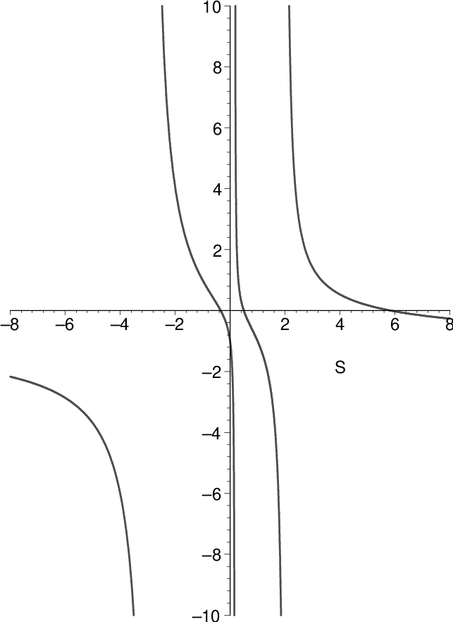
Real roots of (22). An elementary study of the function $R(s)$ , for $s\in{\mathbb{R}}$ , reveals that it consists of 4 decreasing branches, shown in Figure 5 (right), with vertical asymptotes at

s=-\frac{11+3\sqrt{17}}{8}\simeq-2.9,\quad s=\frac{-11+3\sqrt{17}}{8}\simeq 0.17,\quad\hbox{and}\quad s=2.

The branches intersect the $s$ -axis at the reciprocals of these three values (and in particular at $1/2$ ). Thus in ${\mathbb{R}}^{+}$ , the equation $s^{k-1}=R(s)$ has two roots, one below $1/2$ and the other beyond $2$ , which are necessarily the reciprocal of each other. The smallest of these increases to $1/2$ as $k$ increases: thus the corresponding value of $x$ decreases to $0$ as $k$ increases. We denote by $\rho_{k}$ this root of $G_{k}$ .

If $k$ is even, the equation $s^{k-1}=R(s)$ has also two roots in ${\mathbb{R}}^{-}$ . If $k\geq 3$ is odd, the curve $s\mapsto s^{k-1}$ intersects the second branch of $R(s)$ at $s=-1$ , but also somewhere between $s=0$ and $s=-0.508\ldots$ (which is the root obtained for $k=3$ ). The latter intersection point gives rise to a root of $G_{k}$ smaller than $-1$ .

The rest of the argument will show that all other roots of $G_{k}$ lie in $[-1,-1/9]$ .

Roots of (22) of modulus 1. We first observe that, if $s$ has modulus 1, then the same holds for $R(s)$ . More precisely, if $s=e^{i\theta}$ , then $R(s)=e^{i\phi}$ with

	$\displaystyle\cos\phi$	$\displaystyle=$	$\displaystyle-{\frac{56+321\,\cos\theta-336\,\cos^{2}\theta+128\,\cos^{3}\theta}{\left(5-4\,\cos\theta\right)\left(157+44\,\cos\theta-32\,\cos^{2}\theta\right)}},$
	$\displaystyle\sin\phi$	$\displaystyle=$	$\displaystyle-27\,{\frac{\left(29-16\,\cos\theta\right)\sin\theta}{\left(5-4\,\cos\theta\right)\left(157+44\,\cos\theta-32\,\cos^{2}\theta\right)}}.$

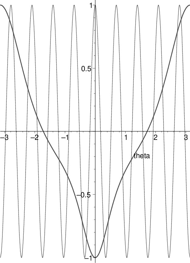
Plots of $\cos\phi$ and $\sin\phi$ as a function of $\theta$ are shown in Figure 6. For $s=e^{i\theta}$ , Eq. (22) is equivalent to $\cos((k-1)\theta)=\cos\phi$ and $\sin((k-1)\theta)=\sin\phi$ . Given that $1/s=e^{-i\theta}$ , we can focus on solutions such that $\theta\in[0,\pi]$ . The oscillations of $\cos((k-1)\theta)$ in this interval imply that the equation $\cos((k-1)\theta)=\cos\phi$ admits at least one solution in each interval $(\frac{m-1}{k-1}\pi,\frac{m}{k-1}\pi]$ , for $1\leq m\leq k-1$ . For each solution, $\sin((k-1)\theta)=\pm\sin\phi$ , and the plot of $\sin\phi$ in Figure 6 shows that $\sin((k-1)\theta)=\sin\phi$ if and only if $\sin((k-1)\theta)\leq 0$ , that is, if $m$ is even. We finally note that, when $k$ is odd, one solution is $\theta=\pi$ , giving $s=-1$ , which we want to exclude.

This discussion shows that (22) has at least $\lceil\frac{k-3}{2}\rceil$ solutions $s\not=-1$ with $\operatorname{Im}(s)>0$ on the unit circle. They give rise to as many roots of $G_{k}$ in the interval $[-1,-1/9]$ . With the two real roots of $G_{k}$ found previously outside this interval, this gives a total of $\lceil\frac{k+1}{2}\rceil$ roots, which coincides with the degree of $G_{k}$ . Hence $G_{k}$ is real rooted, with one positive root $\rho_{k}$ , and the others smaller than $-1/9$ .

In remains to obtain an expansion of $\rho_{k}$ as $k$ grows. We first work out an expansion of the solution of (22) found around $1/2$ (by bootstrapping in (22)):

s={\frac{1}{2}}-{\frac{3}{2^{k+2}}}-{\frac{3}{4^{k+2}}}+\frac{36\,k+27}{4.8^{k+1}}-\frac{{27\cdot 32}\,{k}^{2}-9\cdot 16\,k-717}{16^{k+2}}+O\left(\frac{k^{3}}{32^{k}}\right).

This translates into the expansion of $\rho_{k}$ using (23). The singular behaviour of $M_{k}$ is then derived from (20).

Step 4. Conclusion
By Lemma 7 and Cauchy’s formula,

[x^{\ell}]\left(M_{k}(x)-\frac{\alpha_{k}}{1-x/\rho_{k}}\right)=\frac{1}{2i\pi}\int_{\mathcal{C}}\left(M_{k}(x)-\frac{\alpha_{k}}{1-x/\rho_{k}}\right)\frac{dx}{x^{\ell+1}},

(24)

where $\mathcal{C}$ is the circle of radius $1/9$ centered at the origin. We will prove that there exists a constant $C$ such that for all $k$ and $x\in\mathcal{C}$ ,

\left|M_{k}(x)-\frac{\alpha_{k}}{1-x/\rho_{k}}\right|\leq Ck,

so that (24) implies

[x^{\ell}]M_{k}(x)=\mathbb{E}(X_{k,\ell}^{2})=\alpha_{k}\rho_{k}^{-\ell}+O(9^{\ell}k),

as stated in Proposition 5.

It follows from (14) and (16) that $\frac{\alpha_{k}}{1-x/\rho_{k}}$ is bounded uniformly in $k$ and $x\in\mathcal{C}$ , so that we only need to prove that $M_{k}(x)=O(k)$ , uniformly in $x\in\mathcal{C}$ . By Lemma 6, for any $x\in\mathcal{C}\setminus\{-1/9\}$ , $|S(x)|<1$ . Moreover, $S(x)\rightarrow 1$ as $x\rightarrow-1/9$ . Recall that $M_{k}(x)=2xN_{k}/G_{k}$ . By (17), $N_{k}=2^{k/2}O(k)$ , so that it suffices to prove that $G_{k}/2^{k/2}$ is bounded away from 0, uniformly in $k$ and $x\in\mathcal{C}$ . Since $1+S$ and $S^{k}$ are uniformly bounded, and $P(1/S)$ is bounded away from 0, this is equivalent to

\inf_{k,x\in\mathcal{C}}\left|S^{k}+\frac{P(S)}{P(1/S)}\right|>0.

By the proof of Lemma 7, $S^{k}+\frac{P(S)}{P(1/S)}$ does not vanish on $\mathcal{C}$ . Hence it suffices to prove that

\liminf_{k}\inf_{x\in\mathcal{C}}\left|S^{k}+\frac{P(S)}{P(1/S)}\right|>0.

Let us write $x=-e^{\pm i\theta}/9$ , with $\theta\in[0,\pi]$ . Then, as $\theta\rightarrow 0$ ,

$\displaystyle S(x)$	$\displaystyle=$	$\displaystyle 1-\frac{1}{2}(1\mp i)\sqrt{\theta}+O(\theta),$	(25)
$\displaystyle\|S(x)\|$	$\displaystyle=$	$\displaystyle 1-\frac{1}{2}\sqrt{\theta}+O(\theta),$	(26)
$\displaystyle\frac{P(S)}{P(1/S)}$	$\displaystyle=$	$\displaystyle 1-\frac{20}{13}(1\mp i)\sqrt{\theta}+O(\theta).$	(27)

We split then interval $[0,\pi]$ , to which $\theta$ belongs, in three parts.

$\bullet$ When $\sqrt{\theta}\leq\pi/(2k)$ , there holds, uniformly in $\theta$ ,

S(x)^{k}=\exp\left(-k(1\mp i)\sqrt{\theta}/2\right)+O(1/k).

In particular,

	$\displaystyle\Re(S^{k})$	$\displaystyle=$	$\displaystyle\exp(-k\sqrt{\theta}/2)\cos(k\sqrt{\theta}/2)+O(1/k)$
		$\displaystyle\geq$	$\displaystyle\exp(-\pi/4)/\sqrt{2}+O(1/k).$

Moreover,

\Re\left(\frac{P(S)}{P(1/S)}\right)=1+O(\sqrt{\theta})=1+O(1/k),

uniformly in $\theta$ . Hence

\Re\left(S^{k}+\frac{P(S)}{P(1/S)}\right)=1+\exp(-\pi/4)/\sqrt{2}+O(1/k),

and

\liminf_{k}\inf_{\sqrt{\theta}\leq\pi/(2k)}\left|S^{k}+\frac{P(S)}{P(1/S)}\right|>0.

$\bullet$ Let $\varepsilon>0$ be such that, for $\sqrt{\theta}<\varepsilon$ ,

|S(x)|\leq 1-\sqrt{\theta}/4\quad\hbox{ and }\quad\left|\frac{P(S)}{P(1/S)}\right|>0.9.

Such an $\varepsilon$ exists in view of (26) and (27). For $\pi/(2k)\leq\sqrt{\theta}\leq\varepsilon$ ,

|S|^{k}\leq(1-\sqrt{\theta}/4)^{k}\leq(1-\pi/(8k))^{k}=\exp(-\pi/8)+O(1/k),

so that

\left|S^{k}+\frac{P(S)}{P(1/S)}\right|\geq 0.9-\exp(-\pi/8)+O(1/k)\geq 0.2+O(1/k).

Hence

\liminf_{k}\inf_{\pi/(2k)\leq\sqrt{\theta}\leq\varepsilon}\left|S^{k}+\frac{P(S)}{P(1/S)}\right|>0.

$\bullet$ Finally, when $\sqrt{\theta}\geq\varepsilon$ , then $|S|<1$ is bounded away from 1, uniformly in $\theta$ . Thus, if

\liminf_{k}\inf_{\sqrt{\theta}\geq\varepsilon}\left|S^{k}+\frac{P(S)}{P(1/S)}\right|=0,

there would exist an $x\in\mathcal{C}$ such that $P(S(x))=0$ . But this only happens when $x=0$ or $x=(-1\pm\sqrt{17})/4$ , and none of these values lies on the circle $\mathcal{C}$ .

This concludes the proof of Proposition 5.

4. Back to Knuth’s algorithm

Let us go back to Knuth’s original algorithm, described at the beginning of the paper. Recall that $\mathbb{E}(X_{k})$ is the number of SAWs crossing a square of side $k$ , and that $\mathbb{E}(X_{k}^{2})$ is the sum of the reciprocals of the probabilities of these walks.

Proposition 8.

Denote $c(k)=\mathbb{E}(X_{k})$ and $d(k)=\mathbb{E}(X_{k}^{2})$ . There exist two positive constants $\lambda$ and $\beta$ such that

\mathbb{E}(X_{k})^{1/k^{2}}\rightarrow\lambda\quad\hbox{and}\quad\mathbb{E}(X_{k}^{2})^{1/k^{2}}\rightarrow\beta.

Of course, $\beta\geq\lambda^{2}$ . Moreover,

\lambda=\sup_{k}\ c(k)^{1/(k+1)^{2}}

(28)

and

\beta=\sup_{k}\ (\sqrt{2}\,d(k))^{1/(k+1)^{2}}.

(29)

As discussed at the end of the introduction, there is a hope to combine (29) and known upper bounds on $\lambda$ to prove that $\beta>\lambda^{2}$ , in which case one could conclude that the relative variance of $X_{k}$ grows as $\kappa^{k^{2}}$ , with $\kappa=\beta/\lambda^{2}>1$ .

Proof.

As can be expected, these results follow from a super-multiplicativity argument. The existence of $\lambda$ was established for the first time in [1], and (28) (which allows to produce lower bounds on $\lambda$ ) appears in [7]. We repeat the argument, because it applies almost verbatim to the numbers $d(k)$ .

Define $\lambda:=\limsup_{k}c(k)^{1/k^{2}}$ . Then $\lambda$ is finite, because there are only a quadratic number of edges in the $k\times k$ square, and a walk is determined by the set of its edges. Let $\varepsilon>0$ . We will prove that

\liminf c(K)^{1/K^{2}}\geq\lambda-\varepsilon,

(30)

which implies that $\lambda$ is actually the limit of $c(k)^{1/k^{2}}$ .

Let $k>0$ be such that $c(k)^{1/(k+1)^{2}}>\lambda-\varepsilon$ . Let $K\geq k$ , and let $n$ be maximal so that

(k+1)(2n+1)-1\leq K.

This implies in particular that $K<(k+1)(2n+3)$ . In the $K\times K$ square, put $(2n+1)^{2}$ smaller squares of side $k$ , as shown in Figure 7. In each smaller square, choose a SAW that crosses it, and build from this collection of short walks a long walk crossing the larger square, as shown in the figure. This construction implies

c(K)\geq c(k)^{(2n+1)^{2}}.

Thus

c(K)^{1/K^{2}}\geq c(K)^{1/((k+1)^{2}(2n+3)^{2})}\geq\left(c(k)^{1/(k+1)^{2}}\right)^{(2n+1)^{2}/(2n+3)^{2}}\geq(\lambda-\varepsilon)^{(2n+1)^{2}/(2n+3)^{2}}.

Taking the $\liminf$ on $K$ boils down to taking the $\liminf$ on $n$ and gives (30). The bound (28) also follows from the above inequalities.

Figure 7. Super-multiplicativity for SAWs crossing a square

Let us now consider the numbers $d(k)$ . Again, $\beta:=\limsup d(k)^{1/k^{2}}$ is finite, because

d(k)=\sum_{w\in\mathcal{W}_{k}}\frac{1}{p(w)}\leq\sum_{w\in\mathcal{W}_{k}}3^{|w|}\leq 3^{O(k^{2})}c(k),

where $|w|$ denotes the length of $w$ . Now return to Figure 7. Denote by $w_{1},w_{2},\ldots$ the short walks, and by $w$ the long one. It is clear for the sampling algorithm that

\frac{1}{p(w)}\geq\prod_{i=1}^{(2n+1)^{2}}\frac{1}{p(w_{i})}.

It follows that

d(K)\geq d(k)^{(2n+1)^{2}},

from which one can prove, as above, that $\beta=\lim d(k)^{1/k^{2}}$ . The above bound on $d(K)$ can actually be improved: in every row of $(2n+1)$ small squares, except maybe the top one, $n$ of the horizontal steps added between the small squares have probability $1/2$ or $1/3$ . Hence

d(K)\geq 2^{2n^{2}}d(k)^{(2n+1)^{2}},

and the lower bound (29) now follows.

5. Final comments

5.1. Unconfined walks

Knuth designed his algorithm to sample SAWs crossing a square of side $k$ , but other authors have used similar ideas to sample unconfined SAWs of fixed length $n$ . For example, the classical Rosenbluth algorithm [21] generates general SAWs step by step, by taking at each time, uniformly at random, one of the steps that preserves self-avoidance. If at some point no such step is available, and the walk has not reached length $n$ , the algorithm restarts from scratch. This rejection step is avoided if one only samples untrapped self-avoiding walks, that is, walks that can be extended into a SAW of infinite length⁴⁴ 4 This notion of untrapped walks differs from the one in [19], where a walk is said to be untrapped as soon as it can be extended by one step.. (We describe in Section 5.3 a simple procedure that detects if a new step traps the walk, which is also useful for implementing Knuth’s algorithm.) A recent numerical study, using a refinement of the above algorithm, suggests that the asymptotic properties of untrapped walks are similar to those of general SAWs, in terms of number and end-to-end distance [9].

For these algorithms, the quality of the cardinality estimator is still related to the variance of the random variable $X_{n}$ equal to the reciprocal of the probability of the generated walk. As already mentioned, the variance of the Rosenbluth estimator is predicted to be exponential in $n$ [6]. We do not know of any similar study for untrapped walks. It is easy to determine the variance of $X_{n}$ for the Rosenbluth algorithm restricted to directed or partially directed walks. Our results are summarized in the following table. In particular, for partially directed walks the relative variance is found to be exponential in $n$ .

		North and East	North, East and South	all four steps
confined	number	$4^{k}/\sqrt{k}$	$(k+1)^{k}$	$\lambda^{k^{2}}$
to $k\times k$	rel. var.	$\sqrt{k}$ [5]	$2^{k(k+1)}/(k+1)^{k}$ (Prop. 5)	$\kappa^{k^{2}}$ ? (Prop. 8)
	av. length	$k$	$k^{2}$	$k^{2}$ [16]
unconfined,	number	$2^{n}$	$(1+\sqrt{2})^{n}$	$(2.64...)^{n}$ [17]
$n$ steps	rel. var.	0	$(6/(1+\sqrt{2}))^{n}$	$\alpha^{n}$ (pred. [6])

5.2. Kinetic distributions

It is also interesting to study the asymptotic properties of SAWs chosen according to the non-uniform (but very natural) “kinetic” distribution that results from importance sampling. These properties may be different from those observed in the uniform case. For instance, one can expect the average end-to-end distance of kinetic unconfined SAWs to be smaller than $n^{3/4}$ , because “compact” walks in which few steps are eligible at each time have a higher probability than more spread-out walks. In fact, the kinetic end-to-end distance is conjectured [18] to grow like $n^{2/3}$ . (For unconfined partially directed walks, however, the end-to-end distance is easily shown to be linear, both for the uniform and the kinetic model.) Figure 8 shows a random (untrapped) SAW that we generated by importance sampling and a (quasi-)uniform SAW generated using a pivot algorithm [13].

5.3. When does a walk get trapped?

One important feature of Knuth’s algorithm, and of its adaptation to untrapped SAWs discussed in Section 5.1, is that one never appends a step that would trap the walk. Since Knuth does not explain in his paper how he detects trapping, let us describe the method we used. One obvious case of trapping in Knuth’s algorithm is when the walk reaches the boundary of the square, and moves towards the origin. In all other trapping situations, the walk would have been trapped as well in the unconfined setting, so we focus on the trapping of unconfined walks.

Let $w$ be an untrapped SAW of length $n$ , ending at vertex $v_{n}=(i,j)$ , and, say, with a W step. There are, up to obvious symmetries, exactly three situations when adding a new step to $w$ creates a trapped walk:

•

the vertex $v=(i-1,j)$ belongs to $w$ , one appends a N step to $w$ and the portion of $w$ going from $v$ to $v_{n}$ has winding number $-2\pi$ ,
•

the vertex $v=(i-1,j+1)$ belongs to $w$ , one appends a N step to $w$ and the portion of $w$ going from $v$ to $v_{n}$ has winding number $-2\pi$ ,
•

the vertex $v=(i-1,j+1)$ belongs to $w$ , one appends a W or S step to $w$ and the portion of $w$ going from $v$ to $v_{n}$ has winding number $2\pi$ .

These three cases are depicted in Figure 9. When computing the winding number, we add a half-edge pointing from the East to $v$ (Figure 10). The winding number is then the difference between the number of left turns and the number of right turns, multiplied by $\pi/2$ .

Figure 10. The winding number between

v

and

v_{n}

-2\pi

Acknowledgements. I am very grateful to Persi Diaconis, who first told me about this question, and then sent helpful suggestions on this manuscript and pointed to interesting related papers. I also thank the referee of a first version of this paper for his very thorough report and helpful references.

References

[1] H. L. Abbott and D. Hanson. A lattice path problem. Ars Combin., 6:163–178, 1978.
[2] A. Bacher. Generalized Dyck paths of bounded height. In preparation.
[3] A. Bacher and M. Bousquet-Mélou. Weakly directed self-avoiding walks. J. Combin. Theory Ser. A, 118(8):2365–2391, 2011.
[4] C. Banderier, M. Bousquet-Mélou, A. Denise, P. Flajolet, D. Gardy, and D. Gouyou-Beauchamps. Generating functions for generating trees. Discrete Math., 246(1-3):29–55, 2002.
[5] F. Bassetti and P. Diaconis. Examples comparing importance sampling and the Metropolis algorithm. Illinois J. Math., 50(1-4):67–91 (electronic), 2006.
[6] J. Batoulis and K. Kremer. Statistical properties of biased sampling methods for long polymer chains. J. Phys. A, 21(1):127–146, 1988.
[7] M. Bousquet-Mélou, A. J. Guttmann, and I. Jensen. Self-avoiding walks crossing a square. J. Phys. A, 38(42):9159–9181, 2005.
[8] M. Bousquet-Mélou and M. Petkovšek. Linear recurrences with constant coefficients: the multivariate case. Discrete Math., 225(1-3):51–75, 2000.
[9] Y.-B. Chan and A. Rechnitzer. A Monte Carlo study of non-trapped self-avoiding walks. Preprint 2012. Available at http://www.math.ubc.ca/~andrewr/pub_list.html.
[10] Y. Chen, P. Diaconis, S. P. Holmes, and J. S. Liu. Sequential Monte Carlo methods for statistical analysis of tables. J. Amer. Statist. Assoc., 100(469):109–120, 2005.
[11] P. Diaconis and J. Blitzstein. A sequential importance sampling algorithm for generating random graphs with prescribed degrees. Available at http://www-stat.stanford.edu/ $\sim$ cgates/PERSI/year.html, 2009.
[12] P. Flajolet and R. Sedgewick. Analytic combinatorics. Cambridge University Press, Cambridge, 2009.
[13] T. Kennedy. A faster implementation of the pivot algorithm for self-avoiding walks. J. Statist. Phys., 106(3-4):407–429, 2002.
[14] D. E. Knuth. Mathematics and computer science: coping with finiteness. Science, 194(4271):1235–1242, 1976.
[15] D. E. Knuth. Selected papers on computer science, volume 59 of CSLI Lecture Notes. CSLI Publications, Stanford, CA, 1996.
[16] N. Madras. Critical behaviour of self-avoiding walks that cross a square. J. Phys. A, 28(6):1535–1547, 1995.
[17] N. Madras and G. Slade. The self-avoiding walk. Probability and its Applications. Birkhäuser Boston Inc., Boston, MA, 1993.
[18] I. Majid, N. Jan, A. Coniglio, and H. E. Stanley. Kinetic growth walk: A new model for linear polymers. Phys. Rev. Lett., 52:1257–1260, 1984.
[19] A. L. Owczarek and T. Prellberg. Scaling of the atmosphere of self-avoiding walks. J. Phys. A, 41(37):375004, 6, 2008.
[20] H. Prodinger. The kernel method: a collection of examples. Sém. Lothar. Combin., 50:Art. B50f, 19 pp. (electronic), 2003/04.
[21] M. N. Rosenbluth and A. W. Rosenbluth. Monte Carlo calculation of the average extension of molecular chains. J. Chem. Phys., 23(2):356–359, 1955.
[22] R. P. Stanley. Enumerative combinatorics. Vol. 1, volume 49 of Cambridge Studies in Advanced Mathematics. Cambridge University Press, Cambridge, 1997.

On the importance sampling of self-avoiding walks

Abstract.

Key words and phrases:

1. Introduction

2. Exact results for NES-walks

2.1. The probability p⁡(w)p(w)

Lemma 1.

Proof.

2.2. Enumeration of NES-walks in a strip of fixed height

Proposition 2.

Lemma 3.

Proof.

Proposition 4.

Proof.

3. Asymptotic results for NES-walks

Proposition 5.

Proof.

Lemma 6.

Proof.

Lemma 7.

Proof.

4. Back to Knuth’s algorithm

Proposition 8.

Proof.

5. Final comments

5.1. Unconfined walks

5.2. Kinetic distributions

5.3. When does a walk get trapped?

References

2.1. The probability $p(w)$