Classification of parameter-dependent quantum integrable models, their parameterization, exact solution, and other properties
Abstract
We study general quantum integrable Hamiltonians linear in a coupling constant and represented by finite real symmetric matrices. The restriction on the coupling dependence leads to a natural notion of nontrivial integrals of motion and classification of integrable families into Types according to the number of such integrals. A Type family in our definition is formed by nontrivial mutually commuting operators linear in the coupling. Working from this definition alone, we parameterize Type operators, i.e. resolve the commutation relations, and obtain an exact solution for their eigenvalues and eigenvectors. We show that our parameterization covers all Type 1, 2, and 3 integrable models and discuss the extent to which it is complete for other types. We also present robust numerical observation on the number of energy level crossings in Type integrable systems and analyze the taxonomy of types in the 1d Hubbard model.
I Introduction
Quantum integrability is usually defined as the existence of a sufficient number of nontrivial operators commuting with the Hamiltonian. Such operators are interchangeably referred to as “conserved currents”, “families of commuting Hamiltonians”, integrals of motion, “dynamical conservation laws”, or simply “dynamical symmetries”, and are distinct from the ordinary space-time or internal space symmetries, e.g. momentum and spin conservation, particle-hole symmetry etc. Quantum integrable systems are believed to have a range of properties, which are sometimes proposed as alternative notions or tests of integrability – an exact solution for their eigenstates, Poissonian energy level statistics, level crossings violating the Wigner-von Neumann non-crossing rule in parameter dependent systems, and nondiffractive scattering, see e.g. Ref. 1 for a review.
There are two problems with the above definition. First, it has proved difficult to precisely formulate what constitutes a nontrivial commuting operator. For instance, any Hamiltonian commutes with projectors onto its eigenstates, so the mere statement that there exist commuting operators is not meaningful. In classical mechanics one requires functional independence of the integrals of motion[2]. This criterion is not similarly useful in quantum mechanics where any two commuting matrices are functionally dependent unless there are degeneracies in the spectra of both of them[3]. Second, in a system with a finite Hilbert space we clearly cannot have an infinite number of independent integrals, so we need to specify how many conserved currents are needed to say that the system is integrable. This is especially problematic in systems with no well-defined classical limit, e.g. the Hubbard model on a finite lattice[4, 5], as, unlike the classical mechanics, there is no natural notion of the number of degrees of freedom. There is a similar lack of clarity in delineating the properties of quantum integrable systems. For example, there are poorly understood exceptions to the energy level statistics and level crossing tests[1, 6] as well as no convincing derivation of the exact solution and other properties from the notion of integrability. This is in sharp contrast to the situation in classical mechanics where the Liouville-Arnold theorem[2] demonstrates an exact solution by quadratures and quasi-periodic motion on invariant tori to be direct consequences of integrability.
In the present paper we show that most of these problems can be resolved if one considers Hamiltonians and conserved currents that depend on a real parameter in a certain fixed way. This requirement alone leads to a well-defined notion of quantum integrability allowing us to classify and explicitly construct various integrable models, obtain their exact spectra, as well as derive other properties, directly from their integrability. Examples of such a real parameter, call it , in condensed matter integrable systems are: Coulomb interaction in the Hubbard model, magnetic field in Gaudin magnets with a boundary term[7], anisotropy in the Heisenberg model, interaction strength in the BCS model[8] etc. Dynamical symmetries depend on the same parameter in contrast to ordinary symmetries which are -independent. Cases with no such parameter dependence, e.g. isotropic Heisenberg magnet and Gaudin model in zero field[9], often correspond to a more general integrable model at a specific value of the parameter. In the Gaudin and BCS models the Hamiltonian and all dynamical symmetries are linear in [7, 11, 10], while in the Hubbard and models the Hamiltonian and the first conserved current are linear, while higher currents are higher order polynomials in [12, 13, 14, 15, 16, 17].
Note that in each of the above examples there is a subset of mutually commuting operators, including the Hamiltonian, linear in the parameter. Let us therefore consider Hermitian operators of the form and require the existence of dynamical symmetries linear in . A simple, but important observation is that this restriction on -dependence leads to a natural notion of a nontrivial commuting partner. A typical (“non-integrable”) will commute only with a single (trivial) operator linear in , namely with , where , and are real numbers and is an identity operator. The requirement that there exist a nontrivial commuting partner linear in imposes severe restrictions on . Indeed, as we will see below, a real symmetric for which such a partner exists is uniquely specified by a choice of no more than real parameters, while for a generic one needs real parameters to fix the matrix elements of and [18]. Thus, Hermitian operators with fixed parameter-dependence separate into two distinct classes – those that have nontrivial commuting partners and those that do not.
Further, there is a natural classification of families of parameter-dependent commuting operators according to the number of independent members they contain. Families with the maximum possible number (see below) of such operators we term Type 1, with one less than the maximum – Type 2, etc. The main results of this paper are as follows. First, we construct Type families of commuting operators for arbitrary , i.e. we solve commutation relations for matrix elements of . Second, we obtain exact eigenvalues and eigenstates of each . We thus derive the exact solution from the integrability. Third, we observe that the energy levels of frequently cross and determine the number of level crossings as a function of and . Type 1 (maximal) operators were previously constructed in Refs. 19, 6. Here we analytically obtain all Type 2 and 3 and a sub-class of Type real symmetric operators for arbitrary . In our construction a Type commuting family is parameterized by real parameters, while, as we show, a generic Type involves parameters.
There are typically -independent symmetries common to the Hamiltonian and its dynamical symmetries, e.g. total momentum, particle number, component of the total spin, etc. It makes sense to “factor” all these out, i.e. to go to blocks that correspond to a complete set of quantum numbers. Matrices we construct essentially represent such “irreducible” blocks of integrable Hamiltonians and their dynamical symmetries. As an example, we consider irreducible blocks for the Hubbard model with six sites, three spin-up and three spin-down electrons and determine their types.
A toy version of the above approach to integrability based on studying parameter-dependent commuting matrices was discussed in Ref. 20 in the context of level crossings in the Hubbard model. A major breakthrough came with Shastry’s work [19] where he constructed Type 1 matrices. The advantages of this approach are conceptual simplicity, clear meaning of independent integrals and freedom from specific details of particular integrable systems. A significant disadvantage is that the correspond to isolated sectors/blocks of the Hamiltonian and dynamical symmetries and it is difficult to establish a correspondence between matrices and underlying operators whose blocks they represent. Motivated by Shastry’s work, we proposed a vector space definition (see Sect. II) and the above classification of integrable matrices into types, which allowed us to derive an explicit parameterization for Type 1 matrices, map them to Gaudin magnets and obtain an exact solution for their spectra [6]. Further, we demonstrated that -dependent energy levels of Type 1 matrices have at least one and at most crossings, while levels of integrable matrices of higher types do not have to cross, even though they frequently do.
In what follows we first lay out the general strategy for resolving the commutation relations in Sect. II. In Sect. III we briefly review the Type 1 construction of Refs. 19, 6. Next, we obtain all Type 2 matrices in Sect. IV. In Sect. V we construct integrable matrices of arbitrary Type , which includes and 2 as particular cases. Exact eigenvalues and eigenstates of Type are derived in Sect. VI. Next, we present in Sect. VII ‘gauge’ redundancies in the ansatz parameterization. In Sect. VIII numerical methods for generating random commuting matrices and determining their type, are presented and, thereby, the number of parameters necessary to specify a Type commuting family is determined. In this section we will also discuss whether the construction of Sect. V generates all commuting families. Next, in Sect. IX, we look at the frequent level crossings that occur in Type matrices and relate their number to the properties of the discriminant of the characteristic polynomial of those matrices. We analyze the typology of various Hamiltonian blocks of the 1d Hubbard model in Sect. X. We conclude the main text with the summary and discussion of open questions. Finally, various proofs, details, and tangential results are relegated to appendices A through C.
II Resolving the commutation relations
We start with primary definitions and general observations. First, we define Type operators. As outlined in the introduction, the task of identifying commuting operators linear in a real parameter in matrix representation reduces to finding a certain number, , independent Hermitian matrices such that
| (1) |
Equating terms at all orders of , we have
| (2) |
As discussed above, we also require that there be no -independent symmetry common to all , i.e. there is no such that for all and , where is an identity matrix. When such symmetry is present, acquire block-diagonal structure and the problem reduces to that of smaller matrices. Note also that every commuting family contains the trivial member
| (3) |
where and are arbitrary real numbers.
In light of the restriction on the -dependence, being independent of with simply means linear independence, i.e. with real is zero if and only if all . Note that due to the absence of -independent symmetries linear independence of is equivalent to that of or separately. Further, is defined as the maximum number of independent commuting matrices in a given family. In other words, any that commutes with all is linearly dependent on those same , i.e.
| (4) |
We see that a commuting family is a -dimensional vector space where serve as basic vectors. There is a certain freedom in choosing a basis in the vector space , which will be exploited in Sects. III and IV.
It turns out that a typical matrix of the form has no nontrivial independent commuting partners linear in [6]; it commutes only with and itself. Commutation relations Eq. (1) impose strong constraints on the matrix elements of each such that the probability of finding randomly generated matrices with nontrivial commuting partners is zero. For example, in the case matrix elements of and must meet a single algebraic constraint for such a partner to exist [20] and the number of constraints increases with the size of the matrix. In our experience, finding an operator with even one nontrivial commuting partner is quite difficult. A brute force approach to generating all such operators numerically (see Sect. VIII) already becomes computationally prohibitive for .
Therefore, the minimum (and typical) number of independent in the family is . The maximum possible number can be shown [6] to be , i.e. ranges from 2 to . Following Ref. 6 we term the commuting families with the maximum number of – Type 1, those with commuting operators – Type 2, etc. up to Type . An arbitrary Type family is one with independent commuting matrices , which consist of the trivial independent element and nontrivial ones.
Thus, our task is to identify nontrivial solutions of commutation relations (2). An important observation, which considerably simplifies this task, is that we have freedom to choose bases in two distinct linear spaces without loss of generality. First, we can choose a basis in the “target” space – the Hilbert space on which Hermitian operators and act. Indeed, commutation relations (2) are invariant with respect to transformations , where is any -independent unitary operator. Second, we have freedom to choose a basis in the vector space of commuting operators, i.e. to make linear transformations with any real, -independent and non-degenerate matrix .
It is convenient to choose the basis in the target space to be the common eigenbasis of the mutually commuting matrices . In this basis, are diagonal matrices whose nonzero entries we will denote , i.e.
| (5) |
The commutation relation in this basis reads . This implies that an auxiliary antisymmetric matrix whose matrix elements are
| (6) |
does not depend on , i.e. is the same for all members of the family. Moreover, it follows from Eq. (6) that
| (7) |
where is a diagonal matrix (the diagonal of )[19]. Its nonzero elements we denote ,
| (8) |
Now the commutation relations and are automatically satisfied and Eqs. (2) reduce to a single equation or, equivalently, to
| (9) |
We have, for fixed and , a single matrix “master” equation involving variables – corresponding to and corresponding to – and constraints. In addition to this master equation, we will find that the quantity
| (10) |
is an important one for determining matrix type. We will see that for Type 1, , and for Type 2, where is some real parameter and , are related to the matrix elements of .
Next, let us discuss the choice of basis in the vector space of commuting operators. Note from Eq. (7) that a linear transformation translates into the same transformation on diagonal matrices and and does not affect the matrix , i.e. is independent of the choice of basis in and in this sense is a universal characteristic of the commuting family. Moreover, we will see that for Types 1 and 2 the master Eq. (9) reduces to a single equation on matrix elements of . Once is fully parameterized, and can be determined from Eq. (9). For Type families, we do not attempt to resolve Eq. (9) generally, but use the Type 1 and 2 resolutions to formulate a working ansatz that generates such families.
As mentioned above, linear independence of is equivalent to that of . Given Eq. (5), this means that vectors are linearly independent. Then, via a linear transformation we can go to a canonical basis in the operator space such that of diagonal matrix elements are zero for every . This is the basis we will use for Type 1 and Type 2 families in Sects. III and IV, respectively.
All Hermitian Type 1 matrices were explicitly parameterized in Ref. 6. In constructing higher types here we will restrict our analysis to real symmetric as opposed to general Hermitian matrices for simplicity. Specifically, we will choose the defining parameters of Type commuting families to be real and such that the resulting matrices are real symmetric. We note however that all other properties of Type operators we construct in this paper – i.e. commutation relations (2) and exact solution for the spectra of (see below) – persist even when the parameters are unrestricted complex numbers.
III Review of Type 1 matrices
Here we review the main results for Type 1 [6, 19] – families of commuting operators, linear in a parameter that have a maximum number () of linearly independent members, which were also termed “maximal operators” in Ref. 6. As discussed in the previous section, we can go from a general operator basis to a convenient canonical basis by taking linear combinations of . Since there are linearly independent diagonal matrices in the case of Type 1, we can choose the basis so that all in Eq. (5) are zero except one, i.e. for all .
Consider Eq. (9) in the Type 1 canonical basis. It turns out that the left hand side of this equation is an explicitly mostly empty matrix. Evaluating its nonzero matrix elements, we obtain after some algebra
| (11) |
where are distinct and are the diagonal matrix elements of , see Eq. (8). Consistency requires that a triangular sum of such relations itself vanish, i.e. , from which follows
| (12) |
where is defined in Eq. (10). This is the main equation defining Type 1 matrices[19]. The key insight in Ref. 6 is the understanding that Eq. (12) necessarily implies the parameterization
| (13) |
with unrestricted real parameters and characteristic of the commuting family (see also Ref. 21 for an elegant alternative derivation of Eq. (13) with the help of Plücker relations).
Once the matrix is known, it is straightforward to calculate and matrices with the help of Eqs. (9) and (11). A general Type 1 matrix with arbitrary real takes the form
| (14) |
Eq. (14) provides a complete explicit parameterization of all Type 1 matrices. Note also that the parameterization (14) is independent of the choice of basis in the operator space .
In Ref. 6 we further show that Type 1 operators map onto a sector of Gaudin magnets in the presence of external magnetic field and as a consequence of this correspondence, we use the well known exact solution of the Gaudin model[9, 7, 11] to furnish an exact solution for Type 1. The components of eigenvector of Type 1 matrix are
| (15) |
corresponding to eigenvalue
| (16) |
where the , are subject to a single algebraic equation
| (17) |
An intriguing consequence of this exact solution is that a Type 1 typically multiply violates the Wigner-von Neumann non-crossing rule[22, 23, 24, 25, 26, 27, 28] and, moreover, it is necessary that it do so at least once[6].
IV Complete parameterization of Type 2 matrices
In this section we construct all Type 2 families, i.e. linear vector spaces formed by mutually commuting, independent matrices . The derivation is similar to that of Type 1 in the previous section, but somewhat more involved. We first choose a convenient canonical basis in the operator space as discussed in the end of Sect. II and evaluate matrix elements of Eq. (9) in this basis. This results in an equation constraining the matrix defining Type 2 matrices, which we then solve. The final result – parameterization of Type 2 operators – is given by Eq. (33).
There are linearly independent diagonal matrices for any Type 2 family. Therefore, by taking linear combinations of , we can go to a basis in the operator space where only two of the in Eq. (5) are nonzero. It is convenient to choose and parameterize these nonzero matrix elements as for some fixed and for . We also impose the following constraint on parameters :
| (18) |
so that the identity can be formed by linear combinations of the , thereby ensuring that it is an element of the commuting family.
Eq. (9) in this basis yields
| (19) |
for . Similar to the analogue Eq. (11), consistency requires that a triangular sum of such terms vanish, i.e. , from which follows that . Without loss of generality we can define a quantity such that , which implies that . This relation is general and must be true for all distinct , and therefore consistently permuting indices yields , where is some nonzero real parameter. We therefore obtain
| (20) |
We will show that Eq. (20) can be solved generically. Let us simplify by dividing out the ’s, i.e. let , from which it follows that
| (21) |
We are looking for a parameterization of that resolves Eq. (21), ideally in a manner that treats both of its indices similarly. Our strategy for pursuing this parameterization is to find another equation nontrivially related to Eq. (21) and use that to eliminate some of the ’s. More specifically, Eq. (21) involves four indices whereas the ’s are two index objects – implying that Eq. (21) overdetermines the ’s. We are looking for an equation involving fewer indices from which to derive a parameterization.
The , like the , are antisymmetric and, as it turns out, this property is sufficient to identically satisfy the equation:
Given Eq. (21), we can remove an overall common factor such that
| (22) |
Eq. (22) is now a nontrivial equation constraining the beyond simple antisymmetry. We can use Eq. (21) and Eq. (22) to eliminate . This is the resulting equation
| (23) |
where we have chosen to separate terms involving index and those involving index . Note that both sides of the equation are identical but for the different indices, true for all , and it is for this reason that we can define the object as a two-index quantity though it is defined through quantities involving three indices. From Eq. (23) we obtain
| (24) |
for all . The key result of our strategy is that Eq. (24) implies that
| (25) |
for some parameters .
Again, what we have done here is use the identically satisfied Eq. (22) to reduce a four-index equation (21) to a number of three-index equations involving the index-less parameter and the two-index object . Actually, at this point, there is a simple algorithm to completely determine all ’s. We can fix indices and and choose values for , , and these new parameters , . Given these chosen values, the and can be determined using Eq. (25). Once we have values for and , substitution into Eq. (22) allows us to completely determine , , i.e.
| (26) |
where
and accounts for an inherent ambiguity in sign.
The above algorithm explicitly favors two indices over the others, i.e. the fixed and above, and we would like to treat all indices in a unified way. Let us make the following change of variables: for such that [29], and . By substituting this into Eq. (26) and removing an overall scale (again without loss of generality), we find that
| (27) |
given
| (28) |
where the dependence of on parameters can be determined with a bit of algebra. We are not particularly interested in this functional dependence, however, because Eq. (28) generally satisfies Eq. (21), i.e. if we choose parameters and for , all given by Eq. (27), , satisfy Eq. (21) where in these preferred parameters .
To define the Type 2 fully, we can simply choose of the parameters and determine the remaining one so that Eq. (18) is satisfied. We can, however, write in a more transparent form. Let us introduce new real parameters such that
| (29) |
By partial fraction decomposition
| (30) |
we see that we can impose Eq. (18) by requiring that and be among the solutions to
| (31) |
where is an arbitrary real number and are understood to be distinct. Given Eq. (27) we find that Type 2 take the simple form
| (32) |
Fully parameterizing Type 2 is the lions’ share of the Type 2 parameterization effort and with a bit of algebraic manipulation we determine the , for all using Eqs. (9) and (19), which are linear in . Linear combinations of the resulting yield a general Type 2 matrix
| (33) |
where
| (34) |
and are arbitrary real numbers.
Eq. (33) together with auxiliary Eqs. (28), (31) and (34) provide a complete parameterization of all Type 2 commuting families. independent real parameters , , , and specify the commuting family; real numbers further specify a particular matrix within the family. The choice of all these parameters is unconstrained, except simple explicit restrictions on and to ensure that Eq. (28) produces real , which we discuss in detail in the next section for general Type .
The choice of parameters is not unique. For example, a uniform shift yields the same family. The entire group of “gauge” transformations on the parameters that leave Type 2 commuting families invariant is explored in Sect. VII. Interestingly, it turns out that in the case of Type 2 there is an additional gauge freedom not present for other types, which allows an alternative, particularly transparent parameterization, see Eq. (60).
V Type - the ansatz parameterization
Explicitly constructing the most general Type commuting families is difficult if at all possible (see the discussion Sect. XI for more on this). However, it turns out that the Type 2 formulas of the previous section can be generalized to obtain some Type families with arbitrary . The idea is to use the same Eqs. (32) and (33) to generate the matrices, but to extend Eq. (28) by including more poles in its radicand. Specifically, we take
| (35) |
| (36) |
where , are real numbers and , are solutions of Eq. (31).
In Appendix A we prove that Eq. (33) with and given by Eqs. (35) and (36), respectively, indeed produce Type matrices as defined in Sec. II, i.e. families of linearly independent mutually commuting matrices with no -independent symmetry. Eqs. (33) and (35) contain parameters characterizing the commuting family – ’s and ’s, ’s and parameter . As discussed in detail in Sect. VII, there are certain gauge transformations, such as a uniform scaling of and or a uniform shift of , that leave the commuting family invariant. This allows to fix three degrees of freedom meaning that the number of parameters needed to uniquely specify a Type commuting family produced by our ansatz is . In Sects. VIII and XI we argue based on numerical evidence and other considerations that a general Type family is uniquely specified by parameters. This implies that our construction misses parameters, i.e. it does not yield all commuting families for types .
A natural way to choose a basis for the ansatz Type commuting family is to define the nontrivial such that in Eq. (36) for . For , we take to be proportional to the identity matrix, as given in Eq. (3). In other words,
| (37) |
for . In particular, is a diagonal matrix and
| (38) |
A general member of the commuting family is
| (39) |
consistent with Eqs. (33) and (36), where are arbitrary real coefficients.
Especially interesting in the structure of the ansatz is the form of Eq. (35). The presence of these ’s in Eq. (33) is what essentially distinguishes Type , , from the Type 1 operators reviewed in Sec. III, and therefore what allows for the systematic decrease in size of the commuting family, i.e. these ’s see us go from maximal operator to
| (40) |
for Type . The successive inclusion of poles in the radicand of Eq. (35), i.e. increasing numbers of , incrementally decreases the size of the corresponding commuting family. In particular, two such poles yields precisely the Type 2 matrices of Sect. IV (see in particular Eq. (28)), i.e. for , the ansatz is precisely the complete parameterization of Type 2 given in the previous section.
For , the ansatz offers an alternate, but equivalent parameterization of Type 1 matrices to that given in Eqs. (14). To see this, consider the off-diagonal elements of a general Type 1 matrix given by the ansatz in light of the equation :
| (41) |
we can re-express Eq. (41) in the Eq. (14) form, i.e.
if we have
| (42) |
where are arbitrary real numbers satisfying . Note that this constitutes a threefold redundancy in the ansatz parameterization of Type 1 matrices. In Sect. VII we will see that this redundancy is in addition to another threefold parametric redundancy that all ansatz matrices share. Demonstrating the equivalence of the diagonal elements of maximal matrices as defined by Eqs. (14) to those of ansatz Type 1 matrices, as given by Eqs. (33), proceeds similarly.
The above is sufficient to show that Type 1 matrices, as specified by the above ansatz, are precisely the Type 1 matrices of Sec. III. Note, however, that there is a subtlety in the definition of . In particular, the ansatz seemingly stipulates (i.e. through Eq. (36)) a restricted set of allowed , even for Type 1, whereas the Eqs. (14) take the to be diagonal matrices with arbitrary real diagonal elements . In fact, these are equivalent statements because for there are and in Eq. (36) related via an matrix. This matrix is similar to the Cauchy matrix[31] and can be similarly shown to be nondegenerate. Therefore, for an arbitrary choice of there always exists the corresponding choice of and vice versa.
Note that Eqs. (14), (33) and (35), , are explicitly identical when and all . However, the ansatz allows for some ’s to be when . So for an ansatz Type 1 matrix with – which we might call a ‘Type 0’ matrix – if , has the form Eq. (13). If, however, and , vanishes. It follows that if we take a Type 1 commuting family and tune ever smaller, while keeping all other parameters fixed, we find that when we are left with pseudo-Type 1 matrices with block diagonal structure and, consequently, -independent symmetry. Indeed, these ‘Type 0’ commuting families will be the direct sum of two different Type 1 families.
Ensuring reality of ansatz matrices
Next, we discuss the conditions on ansatz parameters such that the resulting matrices are real symmetric. For unrestricted complex parameters , , , and the above construction, Eqs. (33) and (35), produces complex symmetric matrices for which all properties of Type matrices save for reality, but including the exact spectra derived in the next section hold.
Moreover, it can be shown that there exist complex parameters such that the corresponding matrices are real Type , and where the complexity cannot be removed simply by multiplication by some common factor. A block of the 1d Hubbard model in Appendix C provides an interesting example of such a situation. However, the most general constraint on complex parameters , , , and to ensure real Type matrices appears to be rather non-trivial and we will not attempt to derive it here. Instead, let us choose the parameters and to be real and constrain them so that Eqs. (33) and (35) always yield real matrices. In this case the only problematic component for producing real matrices is the – we still need the radicand in Eq. (35) to be positive.
First, we rewrite the expression under the square root in Eq. (35) as follows
| (43) |
i.e. we traded parameters for new parameters . Note that ’s can be expressed in terms of ’s by computing the residues at the corresponding poles
Let us order so that . Recall that are solutions of Eq. (31). It can be shown (see e.g. Ref. 6) that they are all real and lie between consecutive . We have for and for , where . If we now take , , to be also real and such that
| (44) |
all terms , which is sufficient (though not necessary) to ensure the positivity of the radicand in Eq. 35 and reality of the matrix elements.
VI Exact solution
In this section, we present the exact solution of the Type matrices parameterized by the above ansatz, see Sec. V. The exact solution of the eigenvalue problem for Type matrices proceeds in a manner reminiscent of that of the Type 1 operators of Ref. 6, see also Sec. III. A particularly striking feature of this exact solution is that, though these operators have explicitly more structure than Type 1 operators, the exact solution is nevertheless essentially just as simple, in that the entire eigensolution derives directly from the solution of a single algebraic equation. This is in stark contrast to the situation typical with Bethe’s ansatz where there are a large number of coupled algebraic equations to be solved to derive a small portion of the spectrum.
We want to determine the exact solution , where is a basic operator specified in Eq. (37), and are its eigenvectors and corresponding eigenvalues, respectively. The ansatz eigensolution is as valid for Type 1, as it is for all ansatz Type and so the components of eigenvector must bear some resemblance to that of our existing Type 1 exact solution. Let us modify Eq. (15) somewhat and assume that the component of this eigenvector is given by
| (45) |
Expanding in terms of our parameters and using Eqs. (37) and (40), we obtain, after a bit of algebraic manipulation
Note, the second term is a -dependent coefficient on the putative eigenvector component. This term must vanish in order for Eq. (45) to constitute an eigenvector. Thus, given an eigenvector of matrix specified by Eq. (45) the corresponding eigenvalue is
| (46) |
where is such that the following algebraic equation
| (47) |
is satisfied. We should note, however, that it remains to be proven that Eq. (47) generically yields distinct solutions given both sign choices for , see Eq. (35). Nevertheless, numerical analysis has yielded no counterexample.
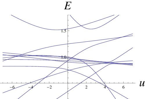
The behavior of the spectrum of a typical Type operator as a function of the parameter is particularly interesting. As distinct from the spectra of random real symmetric operators linear in a parameter, random Type matrices – whose parameters are chosen from random uniform distributions – exhibit frequent violations of the Wigner-von-Neumann non-crossing rule, see Fig. 1, which states that eigenvalues of the same symmetry do not cross as a function of a single coupling parameter.
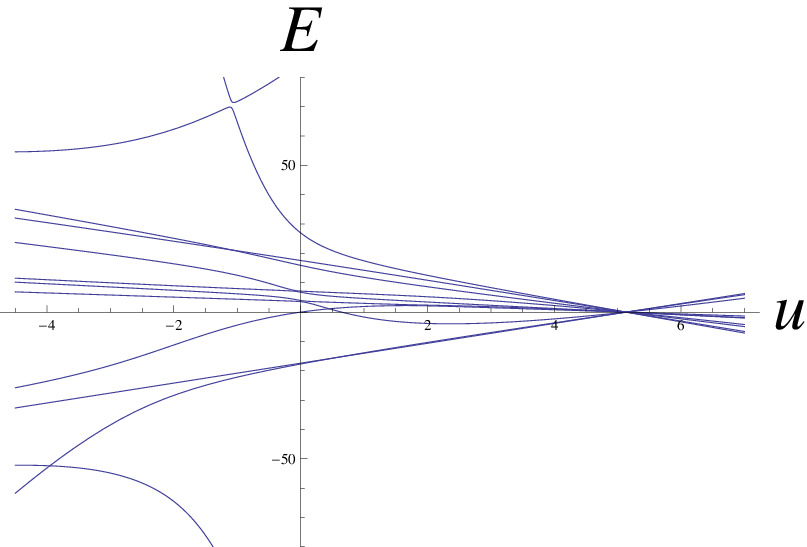
It is interesting to note that numerical observation of individual suggests that they undergo concurrent crossings of eigenvalues at some value of , see Fig. 2. This is a surprising phenomenon that one would rightly expect from Type 2 matrices [30] but, perhaps, not general Type matrices.
We can explain this phenomenon by considering the eigenvalues. At a given , and for all satisfying Eq. (47) we find, through some algebraic manipulation
| (48) |
Thus, at we find that, for , the ’th eigenvalue of is zero. Naturally, not all the eigenvalues can vanish, otherwise is trivial. Indeed, setting and in Eq. (47), we find that it is solved for both sign choices for , i.e. Eq. (47) has a doubly degenerate solution , such that . Numerically, we find confirmation of this phenomenon wherein ’s correspond to zero eigenvalues, while the other two eigenvalues at are non-zero.
VII Gauge redundancy in the ansatz parameters
Given a set of real parameters defining a Type commuting family one might ask whether these parameters are unique, i.e. does there exist a set yielding the same Type commuting family?
On inspection it is apparent that parameters are, in fact, not unique, e.g. a uniform shift of the (and ) parameters leaves Eqs. (33) and (35) unchanged. Similarly, one can find a variety of uniform scaling schemes under which all matrix elements are invariant.
More interesting, however, is the following linear fractional parameter transformation:
| (49) |
where are arbitrary real parameters subject to constraint , and is defined in Eq. (35). It can be shown then that the above transformation yields the corollary transformation:
| (50) |
By direct computation it can be shown that the and, therefore, all off-diagonal matrix elements of the members of the ansatz commuting families are invariant under the above. Now consider the action of this transformation on diagonal matrix elements of basic commuting matrix given by Eqs. (37) and (38). For we have
| (51) |
We see that the effect of the transformation on diagonal matrix is a uniform scaling by and shift by a trace, , i.e.
| (52) |
Using partial fraction decomposition, see Eq. (30), and Eq. (35) it can be shown that
i.e. the gauge transformation preserves the matrix elements of the Type matrices, up to a uniform rescaling, a shift in the coupling parameter and the addition of a multiple of the identity matrix.
Type 2
With respect to the ansatz parameterization, in addition to the invariance under the above transformation, Type 2 matrices have a parametric redundancy not shared by Types . Numerical work undertaken to “reverse engineer” ansatz parameters directly from the matrix elements of commuting matrices produced by the ansatz (see Appendix B) yield back the input parameters, modulo the transformation (49). However, Type 2 matrices exhibit a 1-dim gauge freedom beyond that of Eqs. (49).
To see where this extra redundancy comes from, consider again Eq. (27). Let us now allow to be a smooth function of a parameter such that
| (53) |
where and are defined by the equation
for all . By direct computation it can be shown that is -independent if
| (54) |
i.e. is the elliptic function of corresponding to Eq. (54) with initial conditions . Thus is invariant under the transformation .
A general elliptic function – i.e. one defined by Eq. (54) wherein are arbitrary complex numbers – is related to a specific Jacobi elliptic function through a linear fractional transformation. Concretely,
| (55) |
where are complex numbers such that , and
| (56) |
, and is any one of the four roots of the equation
| (57) |
Elliptic functions have a number of beautiful transformation properties. Interestingly, it can be shown, using the well known ‘angle’ addition formulae involving Jacobi elliptic functions[32] that
| (58) |
where is defined as in Eq. (28) and is one of the characteristic periods of these doubly-periodic functions. This is a surprising intermingling of and , the broader meaning of which remains mysterious.
The most compelling such exploitation of the behavior of Jacobi elliptic functions comes in reconsidering Eq. (53). By directly substituting Eq. (55) into Eq. (53) we find that
| (59) |
However is independent of elliptic parameter . We can make this -invariance manifest by using the addition law properties of Jacobi elliptic functions[32], whereby it can be shown that
| (60) |
where and .
This parametric redundancy is peculiar to Type 2 – the naive generalization to higher types, i.e. extending Eqs. (53) and (54) by including , and generating ’s that satisfy hyperelliptic differential equations does not yield an invariant analogue of Eq. (53). That such a simple, geometric redundancy is embedded in the derived construction of Type 2 matrices is both beautiful and compelling, however its meaning is unclear.
VIII Random generation of commuting matrices and completeness of the ansatz
In this section we address the issue of completeness of the ansatz – whether all Type , commuting matrices are also ansatz matrices, i.e. for any pair of commuting matrices both linear in a parameter , do ansatz parameters and exist that yield back these matrices? As yet, we have no analytic means to directly answer this question, but numerically we find that the answer is ‘Yes’ for and ‘No’ for . Specifically, numerical analysis shows that continuous parameters are needed to uniquely specify a generic Type commuting family, i.e. the ansatz of Sect. V is short by parameters.
Below we will detail this analysis, wherein we
- 1.
generate two random commuting matrices and determine the type of the commuting family they belong to,
- 2.
then process one of these matrices through an algorithm designed to check whether a matrix belongs to an ansatz Type commuting family and extract ansatz parameters if it does.
Recall from Sect. II that any two commuting symmetric matrices and can be represented as and , where are diagonal and is an antisymmetric matrix. is then equivalent to (see Eq. (9))
| (61) |
It turns out that we can generate a pool of generic commuting matrices by brute forcing a solution to Eq. (61). Using Mathematica’s FindRoot[33] function – an algorithm designed to search a -dimensional parameter space for solutions to a set of equations – we input random real values for the nonzero elements of and ask FindRoot to find a solution to Eq. (61) whose matrix elements are close to those of a randomly generated antisymmetric seed matrix. Typically FindRoot is able to quickly find such an antisymmetric matrix. This solution appears to be one of many in a large discrete set of compatible antisymmetric matrices, not all of them real. We know that there are many solutions because changing the random seed matrix, given the same inputs , frequently sees FindRoot land on an entirely different antisymmetric matrix.
We believe the solution set discrete because when Mathematica’s NSolve – an algorithm designed to search for many numerical solutions to an arbitrary set of constraints – attempts to solve Eq. (61) given those same inputs it manages to generate a discrete set of . However if we decrease the number of inputs, e.g. specify only inputs, NSolve very quickly indicates that the system is under-constrained by at least one equation and randomly generates a linear constraint so as to proceed toward calculating a solution set.
In practice, we observe that FindRoot algorithm can find at least one solution to Eq. (61), given inputs. Notice, though, that this method of randomly generating commuting matrices is independent of matrix type, i.e. nowhere in the procedure does one explicitly specify the size of the commuting family to which and belong. The initial parameters defining matrices and the antisymmetric solution matrix correspond to some Type commuting family, and we can determine the value of by counting the number of linearly independent matrices in the commuting family.
In particular we take a putative matrix , where and are diagonal matrices whose nonzero entries, and respectively, are undetermined real variables, and solve commutation relation . There will be equations linear in these unknown and . Let be the number of these equations found to be linearly independent. Then it follows that, because is a Type matrix and, by definition, we can only freely choose of the non-zero matrix elements of and the overall trace of , , i.e. the commutator yields linearly independent constraints on and . Thus counting the number of independent equations tells us the matrix type, .
We observe that this procedure for generating generic commuting matrices yields a distribution of types weighted toward the lower end, see Fig. 3. Interestingly, out of many hundreds of random generations, not one Type 3 matrices was generated, even though we know that they exist and can be readily made by the ansatz.

We cannot as yet prove that given some random diagonal matrices a solution must always exist for Eq. (61), but for the reasons stated above we find empirically that parameters are always sufficient and apparently necessary to generate two distinct commuting matrices. Accordingly, let us assume the correct number of parameters necessary to specify two distinct, generic real symmetric commuting matrices, linear in parameter , regardless of type. If those two matrices are Type , of those inputs are used to uniquely determine the two independent members of the commuting family, i.e. for both unique ’s and an extra inputs to fix a trace on both ’s not constrained by the commutation relations. If, in addition, we remove an overall scale on matrix elements, that leaves of our initial input parameters that remain to uniquely specify a generic Type commuting family.
Are all Type matrices also ansatz?
We already know that all Type and matrices conform to the ansatz – this is essentially what the ansatz was designed to do, see Sects. IV and V. Now let us consider ansatz Type matrices. Counting ansatz parameters and removing the parametric redundancies (see Sect. VII) we are left with parameters to uniquely specify an ansatz Type family. Comparing to the number of parameters needed to specify a generic Type commuting family, we see that ansatz Type families appear smaller by continuous parameters.
These parameter counting arguments strongly suggest that a generic Type commuting matrix is not an ansatz matrix, i.e. the ansatz generates only a small subset of Type for . The case of Type 3 appears marginal, i.e. on the one hand the preceding argument indicates that there are sufficient parameters for ansatz to cover all of Type 3, on the other hand the ansatz is a naive extension on a full parameterization of Type 2 and there is no obvious reason for the ansatz to extend fully to Type 3.
To gain further insight into the completeness of the ansatz, we randomly generate generic commuting matrices of arbitrary type (see above) and subject them to an algorithm (described in detail in Appendix B) that reverse engineers the ansatz parameters from the matrix elements if the matrix is ansatz Type . However, when we run generic commuting matrices through this algorithm, all observed matrices of Type are seen not to be ansatz matrices. In particular, in these cases the algorithm is unable to find nontrivial satisfying Eq. (74).
What is surprising, though, is that the ansatz carries no guarantee that it covers Type , and yet every observed, randomly generated Type matrix has an ansatz parameterization. In view of this result, we conjecture that the ansatz is complete for Types and – which we have proved – and for Type , while incomplete for general Type by an unknown set of parameters, which we note empties for Type . In Sect. XI we provider further arguments supporting this conjecture.
IX Level crossings
One of the signatures of parameter dependent integrable models is the presence of level crossings in their spectra. A general -dependent Hamiltonian, , obeys the Wigner-von Neumann non-crossing rule which states that when one plots the -dependence of those energy levels sharing the same quantum numbers, the levels may approach one another closely, but they never cross[22, 23, 24, 25, 26, 27, 28]. The spectra of Type Hamiltonians, however, behave very differently – they carry frequent (though not necessary[6]) violations of the non-crossing rule, see Figs. 1, 2, and 4.
For Type 1, we were able to offer a topological rationale for the necessary existence of at least one such crossing[6], but the analysis in Type is more difficult. We do observe, however that the number of crossings varies with type as
| (62) |
where is some non-negative integer bounded such that the above expression is non-negative, and where is an integer such that
In the overwhelming number of observed commuting matrices . Specifically, out of several hundreds of matrices analyzed, only two non-ansatz matrices were observed to be such that . then is overwhelmingly identical to type, but there are apparent exceptions (see Sect. XI). Note, we always find for ansatz matrices.
The crossings’ story gets more interesting when one extends the notion of crossings to “complex crossings”, by which we mean complex values of wherein at least two of the eigenvalues of an operator are equal. More concretely, complex crossings occur at values of corresponding to the roots of the discriminant of the characteristic polynomial of . The discriminant is defined as , where are the roots of , i.e. it is polynomial in the coefficients of and, therefore, polynomial in . The order of this polynomial can be shown to be , and, therefore, there are exactly complex values of (roots) where the discriminant vanishes, independent of type or even whether belongs to a commuting family.
However, from numerical analysis we see that for a general these roots do not correspond to eigenvalues being equal one another; they correspond to a situation in which there ceases to be a full eigen-decomposition of the operator. For a completely general, non-integrable matrix, the roots of the discriminant correspond to a spectral decomposition of involving Jordan blocks, rather than eigenspaces, see Ref. 35. A Type matrix, , however, is rather special. Its discriminant – which we denote – factorizes as
where and are polynomials. It turns out that is a polynomial of order and its roots are often real, but not always. Its complex roots come in complex conjugate pairs, hence the term in Eq. (62). All of its roots correspond to values of where at least two eigenvalues are equal. Moreover, if we consider two Type matrices, and belonging to the same commuting family, i.e. , their discriminants will have distinct factors and . However, they will have the same factor and its complex roots correspond to values of where a breakdown of the eigen-structure to Jordan blocks occurs.
Interestingly we also observe that if we express as a polynomial in – which we can do for any pair of non-degenerate commuting matrices, see Ref. 3 – the coefficients of that polynomial are rational functions in the denominators of which are all , i.e.
| (63) |
where are polynomials in of order . Note that the failure of polynomials of a degenerate matrix to span that same matrix’ commutant is reflected in the fact that the above polynomial’s coefficients blow up at the roots of , i.e. at those values of where undergoes a level crossing.

X Taxonomy of types in the 1d Hubbard model
In Sect. VIII we explored the distribution of general and ansatz matrix types among randomly generated commuting matrices. Here we study the prevalence of types in a well-known integrable system. As mentioned in the introduction (Sect. I), sectors of such systems corresponding to a complete set of quantum numbers are Type operators. Our aim is to determine the values of for different sectors and to see if these operators conform to the ansatz of Sect. V.
As an example, we consider 1d Hubbard model on 6 sites, 3 spin up and 3 spin down electrons. Periodic boundary conditions are assumed. The Hamiltonian reads
| (64) |
where and are fermionic creation and annihilation operators, respectively, denotes the spin projection, is the number operator and and are real parameters. There is a hierarchy of conserved currents commuting with each other and with the Hubbard Hamiltonian. The first nontrivial current is linear in both and , while higher currents are polynomials in of order 3 and higher. Following Ref. 34, we choose energy units so that , which is equivalent to the replacement
where is a dimensionless real parameter.
Hamiltonian (64) for 3 spin up and 3 spin down electrons can be represented by a square matrix of size . It has numerous parameter independent symmetries such as total momentum, spin, particle-hole symmetry etc. Using these symmetries, one can bring the Hamiltonian to a block diagonal form with block sizes ranging from 1 to 16; see Refs. 34, 20 for details as well as the quantum numbers corresponding to block sizes shown in Table 1. With the help of this procedure and algorithms described in Sect. VIII and Appendix B, we determine the smallest possible blocks, their type and whether they conform to our ansatz of Sect. V. The results are displayed in Table 1. The total momentum takes integer values in our notation. Spectra for momenta and are identical due to a spatial reflection symmetry. For simplicity, we show the results only for momenta and .
|
| ||||||||||||||||||||||||||||||||||||||||||||||||||||||||
We make the following observations:
- 1.
Recall that Type matrix has nontrivial commuting partners linear in . We note that blocks in Table 1 have 1 to 10 such partners. This implies that the 1d Hubbard model has at least 10 conserved currents linear in , while only one such current has been previously identified. All 10 currents can be written in terms of fermionic creation/annihilation operators with the help of projectors onto the corresponding sectors. The resulting expressions however might turn out to be nonlocal and rather cumbersome.
- 2.
The exact solution of Sect. VI applies to all ansatz blocks in Table 1. Therefore, in all these sectors Bethe’s Ansatz solution for the 1d Hubbard model[5, 36] – a large number of coupled nonlinear equations – reduces to single equation (47). It is interesting to see explicitly how such a simplification becomes possible.
In Appendix C we explicitly write down one of the ansatz Hubbard blocks – the Type 3 block with momentum .
XI Discussion
In this paper, we have defined quantum integrable systems, linear in a parameter , to be operators for which there exist a number of mutually commuting operators similarly linear in . We introduced a classification of these quantum integrable systems according to type, where we defined a Type operator as belonging to a commuting family with linearly independent members. For Types 1 and 2, we were able to resolve the corresponding commutation relations, Eq. (9), yielding a complete parameterization. For higher types, we extended the Type parameterization to create an ansatz, see Eqs. (33)-(36), that parameterizes a subset of all Type commuting matrices. Moreover these ansatz matrices are exactly solvable through a single algebraic expression, Eq. (47).
In addition to this analytic approach to resolving commutation relations, we also brute forced random numerical solutions. We observed that the number of parameters necessary to specify one of these randomly generated commuting families is , whereas the ansatz involves , i.e.
When we attempt to find ansatz parameters that can reproduce a randomly generated commuting family’s matrix elements, we find that this is possible for Types 1, 2, and 3 only; Types do not appear to be ansatz matrices, in general. Interestingly, when attempting to find ansatz parameters for the blocks of the 1d Hubbard model Hamiltonian, we find that a number of them are indeed ansatz. Additionally, we looked at the unusual frequent violations of the non-crossing rule in the spectra of Type matrices and found that the number of (possibly complex) crossings of a Type matrix is precisely the same as the order of a polynomial in whose square is a factor of the discriminant of that matrix’ characteristic polynomial. The other factor of that discriminant is polynomial common to all members of the commuting family, and its roots correspond to complex values of for which all cease to have a full eigen-decomposition, whereby these matrices have nontrivial Jordan canonical form.
The ansatz constitutes a significant step toward a comprehensive theory of parameter dependent finite dimensional integrable models. However, there remains much to be understood about general Type operators. For example, it is believed that there is some to-be-determined equivalence between the existence of parameter dependent conservation laws, and the existence of an exact solution. This relationship is on full display with ansatz Type matrices. However we could, for the sake of curiosity, consider a Type “commuting family” by following the ansatz exactly as written, but taking . Note that this a very degenerate family because the number of independent elements is , i.e. a single nontrivial operator and the identity. At first glance, such matrices do not seem to be different from most parameter dependent matrices in that their only commuting partner is the identity. Nevertheless, these Type matrices are exactly solved by same equations (46) and (47). This suggests that conservation laws linear in the parameter are not necessary for an exact solution, though they may be sufficient. Interestingly, we find numerically that all ansatz Type matrices have commuting currents quadratic in . The exact relationship between these two properties remains elusive.
Most interesting is the question of how the ansatz fails to completely parameterize all Type commuting matrices; i.e. why ansatz Type commuting families involve fewer parameters than generic Type . Parameter counting alone tells us that the ansatz parameterizes all Type 3 matrices, which we have confirmed numerically. Nevertheless, nothing in the derivation of the ansatz necessitates this Type 3 parametric completeness: this result is a complete (albeit pleasant) surprise. But why this surprise coverage of Type 3? Why does the ansatz completely parameterize Type 2 with a redundancy that can be made manifest through elliptic functions?
Let us start with the last question first and let it be the foundation of the following speculation: Type commuting matrices live on compact Riemann surfaces of genus . From this point of view, Type 2 matrices live on tori which, when equipped with a complex structure, become Riemann surfaces of genus 1. Working backward, Type 1 lives on the Riemann sphere. Similarly Type 3 lives on a Riemann surface of genus 2, a complex 2-manifold with two handles, Type 4 a genus 3 surface with three handles, etc.
What do we get for this idle speculation? First, the redundancy of Type 2 ansatz parameters detailed in Sect. VII involves elliptic functions. One way to view such functions is as doubly periodic functions over the complex plane, but another way to understand them is as the basic functions that live on a fundamental parallelogram, where identification of the parallelogram edges implies that these functions live on a complex torus. This alone is a middling justification for such speculation in that it is limited to Type 2.
The Riemann surface conjecture becomes broadly instructive when we further conjecture that ansatz Type matrices live on the hyperelliptic subset of Riemann surfaces of genus . It is a well known result of the study of Riemann surfaces that general surfaces of genus have complex structures parameterized by complex parameters, whereas hyperelliptic Riemann surfaces are much simpler and have complex structures parameterized by complex parameters [38]. If we speculate that the ansatz consistently maps Riemann surfaces of genus to Type commuting families, but that the ansatz is presently restricted to that subset of surfaces that are hyperelliptic, parameter counting tells us that we should be short complex parameters, i.e. that same parameter gap between randomly generated versus ansatz derived Type commuting families. Moreover, it is well known that most Riemann surfaces are not hyperelliptic, but that all surfaces of genus 0, 1, and 2 are—much the same way that the ansatz does not cover most types, but is complete for Types 1, 2 and (apparently) 3.
In future work[37] we will show that the eigenvalues of the ansatz Type matrices belong to the topologically restricted vector space of meromorphic functions on hyperelliptic Riemann surfaces of genus . Moreover, the components of the eigenvectors will also be given by meromorphic functions on these surfaces and we will attempt to generalize the manner in which these functions are determined to arbitrary, non-hyperelliptic Riemann surfaces. There we will see that the well-known Riemann-Roch theorem [38] justifies the correspondence between a Riemann surface’s genus and the commuting family’s type. In particular this theorem will show that the more general genus-type relationship is given by , where the typical situation satisfies the lower bound. From this point of view the fact that sometimes (see Sect. IX) is reflected in the fact that .
XII Acknowledgements
This research was financially supported in part by the National Science Foundation award NSF-DMR-0547769 and by the David and Lucille Packard Foundation.
Appendix A Does the ansatz really parameterize Type ?
Here we prove that the ansatz of Sect. V indeed yields Type families of commuting operators as defined in Sect. II. Specifically, we need to show that: 1) defined by Eq. (37) admit no -independent symmetry, 2) for all and 3) the linear space formed by has dimension , i.e. the only matrices that commute with all are linear combinations thereof.
1. Absence of -independent symmetry. Let us assume such a symmetry exists, i.e. for all and , then
However, for ansatz Type matrices we can choose a basis (38) on such that where, by premise, all are distinct. Consequently an ansatz Type commuting family has a basis in which all diagonal matrices are non-degenerate. It follows then that the only that commutes with all these is itself a diagonal matrix. By directly computing the commutator we see that for to commute with all
where which is only generally satisfied if
for all , i.e. if is a multiple of the identity.
2. Mutual commutativity. Using the relation
and a bit of algebraic manipulation we find that
| (65) |
where
Recall that the satisfy Eq. (31). Given this, it can be shown, using partial fraction decomposition, that
| (66) |
provided are distinct. All terms summed over the index in Eq. (65) contain a factor of the form (66) for and 4, where are by construction distinct. Thus , for all and ranging from 0 to .
3. Dimension of the vector space formed by . Next, we show that there are no members of this commuting family that are linearly independent of . Toward this end, let us consider a general matrix and specifically the diagonal matrix and its nonzero matrix elements . First, we note that if there exists an in the commuting family that is linearly independent of the , , but whose is linearly dependent on the , then there exists a linear combination of and that is both -independent and in the commuting family – a situation precluded by the absence of -independent symmetry demonstrated above.
More generally, in Ref. 19, Shastry shows that for arbitrary (not necessarily ansatz) commuting matrices – independent of type – there exists a necessary (but not sufficient) set of constraints on such that commute with all elements of the commuting family. The constraint is
| (67) |
where and are quantities characteristic of the commuting family as a whole and not specific to any particular one of its members. is defined as in Eq. (12) and is defined as follows:
We have used the matrix elements of to define above, but it turns out that is independent of index . Let us now consider these general quantities as determined by matrix elements given by Eqs. (33) and (35). By direct computation it can be shown that, given the Sec. V ansatz for Type matrices
Now let us compute Eq. (67) expressing as for some . Note this can always be done because the Cauchy matrix is invertible[31]. With so defined, we directly compute Eq. (67) to determine the necessary such that . We find that
which requires that
| (68) |
where summations over and run from 1 to and . Note that terms containing with cancel from Eq. (67) by virtue of identity (66).
For the determinant to vanish, the rows in the matrix in Eq. (68) must be linearly dependent. By the uniqueness of partial fractional decomposition it follows that , i.e. the determinant vanishes if (and only if) does not depend on . Thus we require that
| (69) |
It turns out that the degree of freedom associated with amounts to variation in an overall trace as it can be shown that
| (70) |
independent of the index . Thus, it follows that the only allowed in an ansatz Type family are constrained to be of the form
| (71) |
where and is defined by the right hand side of Eq. (69) with , whereby the ansatz necessarily parameterizes matrices of exactly Type .
Appendix B Inverse problem: determining parameters given an ansatz matrix
Here we detail an algorithm that, given an arbitrary symmetric matrix , determines if it conforms to the ansatz of Sect. V and returns the ansatz parameters when it does.
The algorithm is based on the central observation that the difference between a Type 1 , see Eq. (13), and that of an ansatz Type matrix, see Eq. (40), is the factor . If a Type commuting family has an antisymmetric matrix for which no such factor can be found, we know it does not conform to an ansatz parameterization. If, however, such a factor exists and it can be determined, then we know that
| (72) |
for some and and so defined satisfies the equation
| (73) |
Moreover the reverse is true, i.e. it can be shown that Eq. (73) implies Eq. (72) for some and . Consequently, if Eq. (73) can be solved for , we can essentially strip an ansatz of its factor , and the ansatz parameters and can be determined. Without loss of generality we can multiply Eq. (73) by an overall factor of and look for solutions to resulting equation
| (74) |
This is a massively overdetermined set of equations, quadratic in the terms . We note that the equations are actually linear and homogenous in the terms and that it is possible to attempt solving for the by first finding the minimal set of linearly independent linear equations in and then solving for . In numerical practice, however, Mathematica’s NSolve – programmed to find all sets that satisfy the equations of Eq. (74) – quickly finds nontrivial values for the directly from the overdetermined quadratic equations, if they exist. We find that for matrices with a generic, non-ansatz , solving Eq. (74) yields only trivial solutions, e.g. , for all but one. For ansatz matrices where , however, there are two equivalent, inversely related non-trivial solutions to Eq. (74), i.e.
where are arbitrary complex numbers. Note that having real does not generally guarantee that the corresponding are themselves real. Note also that, despite having proved that Type 1 and 2 matrices always have an ansatz parameterization, one can just as well attempt to determine their ’s using solutions to Eq. (74). However, in both cases the cannot be determined uniquely. In the Type 1 case, NSolve generates a warning indicating that there are not enough constraints for it to express a solution set and that it must generate three additional constraints in order to proceed; from Sect. V we know that these additional constraints amount to fixing the threefold parametric redundancy unique to Type 1. In the case of Type 2, NSolve generates a warning that it must generate a single constraint to proceed; this corresponds to a single redundancy in the parameterization of Type 2 matrices involving elliptic functions, which we detailed in Sect. VII.
If nontrivial solutions exist, the above procedure determines their values. It follows from Eq. (72) that the resulting satisfy a corollary equation
| (75) |
for some to be determined. This we do by fixing and and choosing arbitrary values for and such that we can use equation
| (76) |
to determine for all . From here, determining is straightforward, i.e.
| (77) |
where we have yet another arbitrary degree of freedom in our choice of . These three parametric redundancies, unearthed by this algorithm, constitute an interesting gauge freedom in all ansatz Type commuting families, see Sect. VII.
If and when the algorithm finds values and for a putative ansatz Type matrix , proceeding to determine ansatz parameters is a matter of determining whether there exists an in the commuting family wherein the nonzero elements of diagonal matrix are of the form
for to be determined by the algorithm, see Sect. V. Recall from Sect. VIII that in determining the size of a random Type commuting family, finding all matrices that commute with reduces to linearly independent equations linear in its commuting partner’s diagonal elements. Of these equations, we know that because there are only independent members of the commuting family, exactly of these equations can be found that involve the alone. Consequently there will be constraints on of the form
where coefficients are determined by the matrix elements of . Solving these simultaneous equations reduces to finding all that satisfy polynomials of order . Generally, such simultaneous equations polynomial have no solution. These ones derived from ansatz matrices, however, have an -element solutions set . To be ansatz parameters, each one must correspond to the same parameter satisfying Eq. (31).
Finding the rest of the parameters is a matter of solving overdetermined linear equations
see Eq. (35). If the algorithm can determine these , is ansatz. Failure to determine any of these parameters uniquely (up to the aforementioned gauge redundancy), or any inconsistency with respect to the ansatz equations indicates that the matrix is not ansatz. For example, it is possible that the algorithm could find some and parameters given some matrix, and yet fail to have a consistent ansatz parameter . In practice, however, all matrices tested through this algorithm failed to yield ansatz parameters at the -stage in so much as the algorithm could not find nontrivial consistent with Eq. (74). That is, if there are non-ansatz Type matrices that satisfy Eq. (32) for some not satisfying Eq. (35), they appear to be rather rare in a random ensemble of Type matrices.
Appendix C An example of a sector of the 1d Hubbard model described by the ansatz
Here we explicitly write down the , momentum block of the 1d Hubbard model, which is an ansatz Type 3 matrix, see Sect. X. This block is of the form , where is diagonal matrix with the following entries:
| (78) |
and
| (79) |
Using the procedure outlined in Appendix B, we find the corresponding ansatz parameters
and
References
- [1] J.-S. Caux, J. Mossel, J. Stat. Mech. P02023 (2011).
- [2] V. I. Arnold, Mathematical Methods of Classical Mechanics, (Springer-Verlag, New York, 1978).
- [3] H. Baumgrtel, Analytic perturbation theory for matrices and operators, p. 89 (Birkhuser Verlag, 1985).
- [4] J. Hubbard, Proc. Roy. Soc. A 276 238 (1963).
- [5] F. H. L. Essler , H. Frahm, F. Göhmann, A. Klümper, and V. Korepin, The One-Dimensional Hubbard Model (Cambridge University Press, Cambridge, 2005).
- [6] H. K. Owusu, K. Wagh, and E. A. Yuzbashyan, J. Phys. A: Math. Theor. 42, 035206 (2009).
- [7] E. Sklyanin, J. Sov. Math. 47, 2473 (1989); Progr. Theoret. Phys. Suppl. 118, 35 (1995).
- [8] J. Bardeen, L.N. Cooper, and J.R. Schrieffer, Phys. Rev. 108, 1175 (1957).
- [9] M. Gaudin, Note CEA 1559, 1 (1972); J. Phys. (Paris) 37, 1087 (1976); La fonction d’onde de Bethe, (Masson, Paris, 1983).
- [10] Cambiaggio, M. C., A. M. F. Rivas, and M. Saraceno, Nucl. Phys. A 624, 157 (1997).
- [11] J. Dukelsky, S. Pittel, G. Sierra, Rev. Mod. Phys. 76, 643 (2004).
- [12] B. S. Shastry, Phys. Rev. Lett. 56, 1529 (1986); ibid. 56, 2453 (1986); J. Stat. Phys. 50, 57 (1988).
- [13] M. Lüscher, Nucl. Phys. B117, 475 (1976).
- [14] H. Grosse, Lett. Math. Phys. 18, 151 (1989).
- [15] M. P. Grabowski and P. Mathieu, Ann. Phys. 243, 299 (1995).
- [16] H. Zhou, L. Jiang, and J. Tang, J. Phys. A: Math. Gen 23, 213 (1990).
- [17] B. Fuchssteiner, in Symmetries and Nonlinear Phenomena, p. 22Ð50 (World Scientific Publishers, Singapore, 1988).
- [18] Up to an arbitrary -independent orthogonal transformation (e.g. to a basis where is diagonal), which adds parameters in both cases.
- [19] B. S. Shastry, J. Phys. A: Math. Gen. 38, 431 (2005).
- [20] E. A. Yuzbashyan, B. L. Altshuler and B. S. Shastry, J. Phys. A: Math. Gen. 35, 7525 (2002).
- [21] B. S. Shastry, J. Phys. A: Math. Theor. 44, 052001 (2011).
- [22] F. Hund, Z. Phys. 40, 742 (1927).
- [23] J. von Neumann, E. Wigner, Z. Phys. 30, 467 (1929).
- [24] E. Teller, J. Phys. Chem. 41, 109 (1937).
- [25] L. D. Landau and E.M. Lifshitz, Quantum Mechanics: Non-Relativisitic Theory, pp. 304-305 (Pergamon Press, Oxford, 1980).
- [26] H. C. Longuet-Higgins, Proc. R. Soc. A 344, 147 (1975).
- [27] K. R. Naqvi, W. B. Brown, Int. J. Quantum Chem. 6, 271 (1972).
- [28] J. P. Kestner, L.-M. Duan, Phys. Rev. A 76, 033611 (2007).
- [29] We choose this condition because with the four parameters there is a redundant overall scale. Choosing fixes that scale and, as it turns out, simplifies a number of calculations.
- [30] As explained in Sect. II, in the canonical basis each Type basic operator at is a diagonal matrix with zero eigenvalues.
- [31] S. Schechter, Mathematical Tables and Other Aids to Computation 13 (66), 73 (1959).
- [32] M. Abramowitz and I. A. Stegun, Handbook of Mathematical Functions with Formulas, Graphs, and Mathematical Tables, Ch. 16, pp. 567-581 (New York: Dover, 1972).
- [33] S. Wolfram, The Mathematica Book (Wolfram Media, Champaign, IL, USA, fifth edition, 2003).
- [34] O. J. Heilmann and E. H. Lieb, Ann. N. Acad. Sci. 172, 583 (1971).
- [35] R. A. Horn and C. R. Johnson, Matrix Analysis, pp. 121-142 (Cambridge University Press, Cambridge, 1985).
- [36] E. H. Lieb and F. Y. Wu, Phys. Rev. Lett. 20, 1445 (1968); Erratum, ibid. 21, 192 (1968).
- [37] H. Owusu, unpublished.
- [38] R Miranda, Algebraic Curves and Riemann Surfaces (Providence, RI, American Mathematical Society, 1995).