How to be causal: time, spacetime, and spectra
Abstract
I explain a simple definition of causality in widespread use, and indicate how it links to the Kramers Kronig relations. The specification of causality in terms of temporal differential eqations then shows us the way to write down dynamical models so that their causal nature in the sense used here should be obvious to all. To extend existing treatments of causality that work only in the frequency domain, I derive a reformulation of the long-standing Kramers Kronig relations applicable not only to just temporal causality, but also to spacetime “light-cone” causality based on signals carried by waves. I also apply this causal reasoning to Maxwell’s equations, which is an instructive example since their casual properties are sometimes debated.
I Introduction
Causality11
1
Published in Eur. J. Phys. 32, 1687 (2011),
subsequently updated here.
Statement required by the publisher of the EJP:
This is an author-created, un-copyedited version of an article
accepted for publication in the European Journal of Physics.
IOP Publishing Ltd is not responsible for any errors or omissions
in this version of the manuscript or any version derived from it.
The definitive publisher-authenticated version is available online at
doi:10.1088/0143-0807/32/6/022.
is a basic concept in physics -
so basic,
in fact,
that it is hard to conceive of a useful model in which effects
do not have causes.
Indeed,
the whole point of a physical model could
be said to describe the process of cause and effect
in some particular situation.
But what do we generally mean by word like “causality”,
and phrases such as “cause and effect”?
Usually,
we mean that the cause of any event
must not be later than any of its effects.
But even such simple-sounding statements
are rarely as uncomplicated as they seem:
when trying to clarify the details and built-in assumptions,
it is easily possible to get into philosophical discussions
[1, 2],
issues regarding statistical inference and induction [3],
or particular physical arguments [4].
Here I instead follow the physics tradition
characterized
by Mermin as “shut up and calculate” [5].
But what should we calculate,
and how?
Note that common expressions such as do not express a causal relationship in the sense used here. They provide no means of telling whether the force is supposed to cause an acceleration , or cause , or even if the equation is instead intended as a constraint of some kind. Instead, we start with differential equations containing temporal derivatives, which are open-ended specifications for the future behaviour. They require only a knowledge of initial conditions and the on-going behaviour of the environment to solve.
Additionally, since any effect must not occur before its cause , a mathematical expression for must become non-zero only after that cause. This desired behaviour matches that of the mathematical step function , which has for , and for . The definition of causality applied by this temporal step function is the same as that enforced in the frequency domain by the famous Kramers Kronig relations [6, 7]. Therefore I call the time-step causality discussed here “KK causality”, to distinguish it from alternative definitions.
After describing the role of differential equations and how they can generate the time-step criteria in section II, I consider causality in the spectral domain in section III, and discuss typical models in section IV. Causality and Maxwell’s Equations is discussed in section V, followed by the development of a new spacetime formulation of the Kramers Kronig relations in section VI. After a discussion in section VII, I summarize in section VIII. There are also two appendices (A and B) – not present in the published version – which consider the results of section II applied to discretized (or numerical) models, and then the role of spacetime transformations when attributing of causes and effects.
This undergraduate level presentation introduces causality as a topic in itself, making specific reference to the construction of causal models, rather than being a brief diversion on the way to discussing the Kramers Kronig relations, as is the case in many textbooks. It details the connection between time and frequency domain representations and then extends this to a full spacetime “wave-cone” causality. I envisage that this discussion could be incorporated most easily into relativity or electromagnetism courses, although parts could be integrated into courses on mechanics or wave motion.
II Causal differential equations
Let us first write down a simple model, where some system responds to its local environment . Here can be any quantity – e.g. a position or velocity, a level of excitation of some system, and even – if a position is also specified – a probability distribution or wave function. Likewise might be anything, depending on some pre-set behaviour, the behaviour of or other systems, or (e.g.) spatial derivatives of fields, potentials, distributions, and so on. Whatever the specific meaning of (or indeed of ), we start by writing the simplest possible differential equation22 2 See also e.g. [8, 9] for mathematical details..
| (1) |
where is just the time derivative . To determine how causal this model equation is, consider the case where the environment contains a simple possible cause: a brief delta-function impulse, where . Reassuringly, if I integrate eqn. (1), then will gain a step at – i.e. the effect of the impulsive is to cause to increase discontinuously by at ; as depicted on fig. 1. Thus we see how the step function arises directly from the most basic temporal differential equation. If we apply as a filter to , but it changes nothing (in the example above, ), then we know that is causal, since all effects occur after the cause .
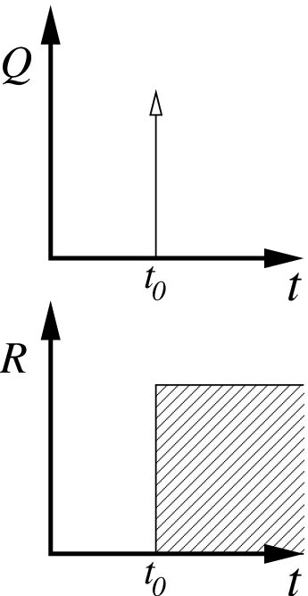
I describe this situation, where an impulse gives rise to a stepped response as “barely causal”, because part of the effect is simultaneous with the cause. Other responses (e.g. see section IV) are usually more complicated and contain higher-order time derivatives, leading to a more gradual response. E.g., a differential equation with second order time derivatives has a ramp-like (linear) response to a delta function cause, whereas third order derivatives give a quadratic response.
Simple examples from kinematics can illustrate the meaning of “causal” as used here. If we were to write down , then we could make the statement that “velocity causes a change in position ”; likewise means that “acceleration causes a change in velocity ”; and means “acceleration causes changes in position ”.
More general differential equations can be written down as weighted sums of different orders of time derivatives e.g.
| (2) |
for parameters , , and a defined maximum order of derivatives , with . These will remain KK causal as long as the highest derivative on the RHS is of lower order than that on the LHS [10].
We might consider recasting the differential equations used here in an integral form; e.g. for an evolution starting at a time , eqn. (1) becomes
| (3) |
although in most cases this is not as easy as writing down the differential equation. Also, as discussed next, differential equations make it easier to consider the spectral properties. And on a more intuitive note, writing down a differential equation does not imply you have solved it – it is a notation more compatible with the concept of an unknown future outcome, dependent on as-yet unknown future causes [11]. This point of view becomes clearer when discretized forms of the differential models are considered, as done in the appendix (Appendix A: A discrete picture). Further, the ambitious may find it interesting to consider the causal set approach [12] to how a universe universe extends itself into its future.
III Causality and spectra
Often, the more complicated a model response is, the more likely it is that its response will be analyzed in the frequency domain. This might be either because an experiment has recorded spectral data directly, or time varying data has been converted into a spectrum using a Fourier transform [13, 14]. Although it is common to write down the individual sin and cosine Fourier transforms, it is most convenient to combine them using , giving
| (4) |
Note that even for real-valued , the spectrum can be complex valued. If is consistent with casuality, then its spectrum must also, and this insistence that measured spectral data must be consistent with causality can be of considerable use [15]. So useful, in fact, that even quite long articles on causality and spectra [16] can get away without any discussion of time-domain dynamics at all!
Let us therefore take our simple eqn. (1) and either Fourier transform it, or take the mathematical shortcut of assuming an time dependence. Since transforms to , we get
| (5) | ||||
| (6) |
If is a delta function, then its spectrum is a constant with , so that
| (7) |
Since we already know that the solution for contains a step at , then we now also know (and can check) that the Fourier transform of a step function is proportional to . Returning also to the more general differential form in eqn. (2), we see that since the LHS has higher order time derivatives than the RHS, any rearrangement to put only on the LHS (as in eqn. (7)) will result in an RHS that falls off at least as fast as .
An important and useful way of checking and /or enforcing causality on spectra are the Kramers Kronig (KK) relations [6, 7, 15]. Although derivations are complicated, their basic construction is based on two concepts:

- 1.
The Hilbert transform [17, 14], is an integral transform that convolves with the step function . This step establishes or enforces the one sided nature of effects that are generated causally:
(a) A cause at can only have effects that appear for times , so that multiplying by has no effect, i.e. , as on fig. 1.
(b) A historical record at a time only contains data on the past (), i.e. , as on fig. 2.
(c) A linear response function , where only depends on past values of . The Fourier convolution theorum then tells us that .
- 2.
The Fourier transform is based on the exponential (see eqn. (4)). It is widely used to re-represent a response , time history , or response function as a spectrum. This requires that the Fourier transforms of , , or are well behaved enough to exist, which usually requires them to be normalizable and to vanish fast enough as .
The Hilbert and Fourier transforms combine to turn time-domain “step” restrictions on the real-valued into spectral constraints on the complex . Following a well known theorem of Titchmarsh [18, 15], we can state that for some causal (i.e. step-like) function which depends only on the past (i.e. ), the real and imaginary parts of its frequency spectrum are connected by
| (8) |
where the prefactor serves to cross-link the real and imaginary parts of ; often the two parts are written explicitly as
| (9) | ||||
| (10) |
The preferred direction for “the past” is set by , for a response or , we set ; for a historical record we use . The operator takes the principal part [19] of the integral, returning what we would get for the integral if those points at which the integrand diverges were skipped. Both eqns. (9) and (10) thus inform us as to the spectral effect of temporal causality. However, it is not necessary to understand the mathematics they rely on – i.e. integral transforms and (complex) contour integration – in order to appreciate their meaning.
What the KK relations tell us is that local properties are tied to global ones, as noted later on fig. 4. If the complex valued represents a response function, then the real part () is the dispersion – in optics, this might be the refractive index change , whose frequency dependence in glass gives rise to differing phase and group velocities [20] for different colours, as well as different angles of refraction. The imaginary part () is then the loss or absorption, or, in amplifying media (as in a laser), the gain. We can then see that the KK relation eqn. (9) links the global loss properties ( for all ) to the response at a specific frequency (). Likewise, eqn. (10) links the global dispersive properties (, for all ) to losses at a specific frequency (). More generally, any effect requiring complicated behaviour for the real part of the spectra (usually described as “dispersion”) usually has an associated imaginary component, which for passive systems can usually be interpreted as loss. This is the origin of commonly made (and not always true) statements along the lines of “dispersion requires (or induces) loss” [21, 22].
IV A driven, damped oscillator
Let us now consider a causal response more complicated than the simple case shown in eqn. (1), but both simpler and more specific than the very general form of eqn. (2). An ideal example is that of a driven, damped oscillator such as a mass on a spring [23, 24], whose temporal differential equation matches that often used in electromagnetism to model the Lorentz response in a dielectric medium [25, 26]. For the mass on a spring, with a spring constant , we have a resonant frequency of , and a friction (or “loss”) parameter ; likewise the Lorentz response also has a resonant frequency and loss. Given these parameters, the displacement of the pendulumn bob (or dielectric polarization ) could then be affected by the driving force per unit mass (or electric field ) according to equations of the form
| (11) | ||||
| (12) |
Here a delta function impulse in force does not induce an initial step change in position, but in velocity ; with the likewise initial response of a linear (or ramp-like) change in position, with . In the same way, in an electromagnetic Lorentz dielectric medium, an impulsive gives rise to an initial step change in polarization current , and a concomittant ramp/linear change in polarization initially, i.e. . Fig. 3 shows some typical oscillating (under-damped) time responses to an impulsive driving force.

Both eqns. (11) and (12) are linear, so that the model can also be expressed in terms of a response function – e.g. for the dielectric, we would have that . We can then Fourier transform this, and when the transform of is denoted , we have that . Since the Fourier transform of eqn. (12) is
| (13) |
the spectral response is then easily obtained, being
| (14) |
whose real and imaginary parts are shown on fig. 4. In an electromagnetic dielectric is related to the refractive index by [20]. We can see from eqn. (14) that the real part of has a frequency dependent variation with an explicit dependence on the loss parameter . Likewise, the loss-like part of the response, i.e. the imaginary part of , has an explicit dependence on frequency.

Not all models that we might derive or write down will be causal. A contemporary example is the F-model [27], which is used to describe the magnetic response (i.e. the magnetization ) of the split-ring resonators (SRRs) often used in electromagnetic metamaterials. While similar to the Lorentz model, its driving term is instead the second derivative of the magnetic field. At frequencies relevant to typical applications, the F-model works well; but for high frequencies where , the associated short wavelengths cause the approximations used to derive it to fail. The F-model follows
| (15) |
The spectral response based on or is
| (16) |
This isn’t KK causal, because eqn. (15) violates the criterion of having lower-order time derivatives on the right as compared to the left, and (therefore) eqn. (16) fails the test imposed by the Kramers Kronig relations: the response remains finite at arbitrarily high frequencies. More descriptively, we can say that ever higher frequency components of and become ever more synchronized; and synchronized quantities are related not by cause-and-effect, but with an equality.
We can, however, fix the F-model by defining a new auxiliary field . This separates the changes in caused by , from those synchronized with , by allowing us to merge the two highest-order derivative terms. The resulting explicitly causal F-model, where and cause changes in , is now compatible with eqn. (2), and follows
| (17) |
which has a spectral response based on or . It vanishes correctly at high frequencies, and is
| (18) |
We can use either of eqn. (17) or (18) to evaluate , after which we can extract and find using and the constitutive relation . Although re-expressing the F-model in terms of does not alter the many physical approximations made in its derivation, by shifting the non-causal part into the constitutive relation for (an equality), it ensures that the dynamic response in eqn. (17) is now explicitly causal.
V Maxwell’s equations
The curl Maxwell’s equations control the behaviour of the electric and electric displacement fields and , and the magnetic and magnetic induction fields and ; and depend on a current density . Although usually written with the curl operator on the LHS [25, 26], our simple causal model of eqn. (1) leads instead to
| (19) |
These otherwise independent pairs and [28] are connected together by the constitutive relations involving the dielectric polarization and magnetization of the background medium, which are
| (20) |
and are subject to the constraint imposed by the divergence Maxwell’s equations, which depend on the free electric charge density and the zero magnetic charge density, and are
| (21) |
Perhaps surprisingly, the causal nature of Maxwell’s equations remains a subject of debate (see e.g. [29, 30]). Nevertheless, the curl Maxwell’s equations must be causal in the “step” KK sense: eqns. (19) have the same form as our simple causal model in eqn. (1). The curl operators, by specifying how the spatial profile of and drive changes in and , turns them into wave equations when combined with the constitutive relations. Take as a starting point the case in vacuum, where and are both zero, so that and . Then we can then rewrite eqns. (19) solely in terms of any pair of electric-like ( or ) and magnetic-like ( or ) fields; e.g.
| (22) |
which can be combined into second order forms for or , e.g. . While these vacuum Maxwell’s equations are self-evidently KK causal, more generally, the background medium for the electromagnetic fields can have non-trivial and dynamical responses to those fields encoded in and . To avoid specifying particular response models, I represent all possible causal differential equations for and (compatible with eqn. (2)) with the notation
| (23) |
As an example, might be used to represent eqn. (12), the Lorentz response in a dielectric.
A straightforward expression of Maxwell’s equations that emphasizes their causal nature is achieved by insisting that any given field should not appear on both the LHS and RHS of the equations. Thus every field that has a dynamical response (i.e. is modelled by a temporal differential equation) can be updated simultaneously. There is no need to follow some specified sequence, although that can be useful, as in e.g. finite element simulations [31]. We can even do this even whilst incorporating magneto-electric material responses, where the electric field affects the magnetization, or the magnetic field affects the dielectric polarization. Maxwell’s equations, written to fit these criteria, are
| (24) | ||||||
| (25) |
Although interdependent, these equations remain explicitly KK causal in the sense that and are uniquely defined as causes, and and are affected by those causes (i.e. show “effects”). Further, we cannot regard the displacement current (or indeed its magnetic counterpart ) as “causes” in the manner reviewed by Heras [32]; these changes in and are instead effects.
In typical non magneto-electric cases, where and , the two equation sets (24) and (25) are independent of one another. This further possible separation is the reason for associating the equation for with that for in eqn. (24), and associating that for with in eqn. (25).
Once the RHS’s of eqns. (24) and (25) have been evaluated, the LHS’s can be integrated directly in an explicitly KK causal manner – the “cause” fields have had effects on and . Then, the usual constitutive relations can be rearranged to connect the fields according to
| (26) |
to allow us to directly update the the “cause” fields and .
Note that if the evolution of or were (e.g.) to be written as dependent on or , (so that ), then there is no longer a perfect separation between “cause fields” and “effect fields”. Nevertheless, such a rewriting will not violate causality, since the differential equations still have the correct form.
We can easily replace the abstract current density by incorporating the motion of a particles of mass and charge at position with velocity , by using additional causal equations
| (27) | ||||
| (28) |
along with the connection between the electric current density and the particle motion, and the charge density, which are
| (29) | ||||
| (30) |
Of course, how light changes its propagation properties inside some material is not always described using charges, currents, or polarization and/or magnetization. Instead we often use its refractive index , which has two distinct contributions. First, there is the vacuum or spacetime metric component, which is unity at all frequencies; it is this part that was historically interpreted as an instantaneously responding electromagnetic “ether”. Second, there is that due to the polarization and magnetization responses (i.e. either or [20]), and it is this second component which causality (and the KK relations) insist should vanish at high frequencies.
Finally, note that this approach can be also be applied to Faraday’s Law, which result in some perhaps surprising conclusions [33].
VI Waves and signals
Causality can be broadened to include the notion of “signal causality” – where signals must pass between two separate points for influences to be felt. To analyse this problem, I take the postion that signals are sent using waves, and that waves follow wave equations. This is motivated by the important case of lightspeed signals, as propagated according to Maxwell’s equations. We will see that light propagation is not only “time-step” KK causal as discussed in section V, but “wave-cone” (light-cone) causal as well.
To start, let us convert our simple causal differential equation (1) into a wave equation by augmenting the cause by a spatial derivative of the effect and a wave speed , e.g.
| (31) |
where is just the spatial derivative . Thus we can see that waves are (at least in part) their own causes, where in particular the “cause” of changes in profile is their own pre-existing spatial modulation, in addition to any source-like causes . To obtain bi-directional propagation we need either higher order derivatives or multi-component waves, e.g. in three dimensions we need at least one scalar and one vector component. As for linearized acoustic waves in pressure and fluid velocity [34], we could link a scalar and vector with a pair of differential equations:
| (32) | ||||
| (33) |
These can be combined into either of two second order forms, the scalar one being the simplest, which with and is
| (34) |
This is explicitly KK causal, since the LHS has a second order time derivative, whilst the RHS has at most only a single time derivative inside . Many other wave models are possible, notably the transverse electromagnetic waves generated by Maxwell’s equations (see section V), for which a very general second order form comparable to eqn. (34) exists [35]; as well as a first order bidirectional version [36]. The hyperbolic form of these second order wave equations gives rise to “wave-cones” analogous to the light cones discussed in relativistic scenarios.
Most simple linear waves follow second order equations like eqn. (34), although different physical properties are denoted by and in the different cases. Such waves provide a useful basis for analysing causal signalling, since they can be used to establish KK relations that constrain spectra in both space and time. It is important to choose as a basis those waves travelling at the fastest relevant signal speed. Of course the speed of light can always fulfill this role, but there may be cases when a lower speed limit is appropriate [37].
In special relativity, one important frame independent quantity for any two spacetime points (i.e. here the origin and ) is the interval between them [38]. It also plays a crucial role in spacetime causality, since it is equally useful for waves in an isotropic material medium, as long as we remain in the rest frame of that medium. The interval is
| (35) |
Here I have used the sign of to distinguish positive intervals (between now and points in the future wave-cone) and negative intervals (between now and points in the past wave-cone); imaginary values of , resulting from , are excluded. We also need a rapidity coordinate
| (36) |
which indicates the average speed required to travel between a point and the origin. How these relate to , coordinates is shown on fig. 5. The inverse transformation is
| (37) | ||||
| (38) |
In special relativity, where is the speed of light, and are related to the Rindler coordinates, but are for timelike intervals rather than spacelike ones. To complete the coordinate set, we need the two polar angles that enable us to reconstruct the individual position coordinates from their magnitude ; using and . For notational convenience, we can combine with to form a single rapidity vector ; we might also define pseudo-Cartesian coordinates with , , and to give .

In the 1D linear case with and , or the spherically symmetric case with , the wave equations in both sets of coordinates are
| (39) | ||||
| (40) |
where the source terms are written simply as a , even though they vary between cases. The critical difference between the coordinates and the ones is that for the latter choice, the edge of the wave-cone is coincident with and is never crossed. Thus “spacelike” intervals are not covered by these hyperbolic coordinates. As a result, only the wave interval has causal restrictions. And whilst eqn. (39) is explicitly time-step or KK causal, eqn. (40) is something more – it is wave-cone causal (or, as named below, KK causal).
When considering the wave equations (39) and (40), note that the eigenfunctions of , , or are just plane waves (e.g.) with eigenvalues . In contrast those of are powers of , where eigenfunctions have eigenvalues . This means that while the Fourier transform is the natural choice for a spectral transformation on , , or , it is not so for . In fact the power-law dependence of the eigenfunctions for indicates that the Mellin transform [39, 14] should be the natural choice.
Nevertheless, the mathematical construction of the KK relations depends only on having a step function along some coordinate. Thus we can still use the Fourier transform to construct spacetime KK relations, and so avoid for now using the lesser known Mellin transform. Taking the Fourier spectral counter part of to be , we can rewrite eqn. (8) and get a KK relation consistent with the signal causality resulting from the wave equation (34). Thus for a wave, or some wave-causal quantity , we have the KK relations
| (41) |
Further, we can also consider the -spectral version of eqn. (41); where we denote the wavevector-like counterpart of the rapidity by the symbol . Since is unbounded, Fourier transforming into the domain gives the doubly transformed , satisfying KK relations
| (42) |
where . Of course, the angular coordinates could also be transformed into angular spectra, or we could start with the pseudo-Cartesian and transform into its spectral counterpart .
Looking back at the definition of , we see that for pointlike objects, the standard KK relations might still be applied, since whatever variation in there is merely compresses differently with respect to , leaving the step function intact. Nevertheless, discrepancies between true spacetime KK causality and simple temporal KK causality will exist; e.g. most simply, a pointlike object moving with fixed rapidity will have its frequencies scaled by a factor of due to time dilation.
More remarkable is what eqn. (42) says about the spatial (wavevector) spectra. Only for a narrow range of fixed times in the past, where an object is well localized inside the wave-cone (so that and ), can an ordinary spatial spectra based on an be made to match up with the (wave-cone) rapidity spectra based on . Nevertheless, in typical, non-relativistic, laboratory situations with lightspeed communication, we can quite reasonably restrict our analysis to that small region of agreement. Otherwise, our lack of knowledge about the situation outside the wave-cone, and the mismatch between spatial coordinate and the spatiotemporal means that since looks nothing like , their respective spectra , are also utterly different: a structure periodic in is not periodic in .
VII Simultaneity, locality, and smoothness
Two points raised by the stance of Jefimenko [30] question (a) whether the use of local causality is appropriate, and (b) if causes and effects can be simultaneous.
Local vs retarded causes: The local causality used here works knowing only the current state and current influences, and makes only minimal assumptions. In contrast, some (e.g. Jefimenko [30], also see Heras [32]) prefer to relate effects back to their original causes. Thus the electromagnetic fields would be directly obtained from the integral equations over the past behaviour of charges and currents (see eqns. (7,8) in [30]). From a practical perspective, this can raise difficulties: we often want to solve electromagnetic problems for free fields on the basis of some stated initial boundary conditions – where we do not know, nor want to calculate, whatever sources may have been required to generate them. KK causality, being local, neither knows or cares about this “deep” past; but casuality is still enforced and remains testable. However, this deep past is not irrelevant, and the assumption that fields can be related back to sources is an important one [40].
Simultaneity & smoothness: We might take the position that having any part (however infinitesimal) of the effect simultaneous with the cause is unsatisfactory; e.g. as does Jefimenko [30] with regard to Maxwell’s equations, and by implication even the simple eqn. (1), even though both are KK causal (even if they might not be “Jefimenko causal” as well). Mathematically, the step response can be made non-simultaneous by use of rather than , but since this has negligible physical consequences, we might prefer to remove the simultaneity by demanding a smooth response. This can be instituted by replacing the LHS of eqn. (1) with the second order , so that a delta function impulse gives a linear-ramp instead of a step response. Then we would no longer use to say that “velocity causes change in position”, but instead use and say that “acceleration causes change in position”. However, if we demand this, then we find that the curl Maxwell’s equations – with their single time derivative – no longer count as causal; and other wave equations (e.g. (31), (32), (33)) suffer a similar fate.
VIII Summary
KK causal models are constructed as temporal differential equations where the changes with time of the effect depends on the strength of some cause. The simplest possible model is written down as eqn. (1), containing a cause , something to be affected , and a single time derivative applied to . In such a case an impulsive cause leads to a step-like effect. For example, in kinematics, the equation , allows us to make the statement that “velocity causes a change in position ”. In contrast, writing down e.g. does not allow me to claim either that “ causes ” or “ causes ”. But I could instead write and then make the KK causal statement “a given causes a change in velocity ”. This argument then shows that Maxwell’s equations are unambiguously causal in the KK sense, whether or not any useful alternative definitions of causality exist.
It is well known that a spectral analysis of “time-step” causality gives rise to the Kramers Kronig relations, which apply constraints to measured spectral data; and link the real and imaginary parts of the spectra in a global-to-local manner. Here I have broadened the notion of “time-step” KK causality and developed “wave-cone” KKK relations for signal causality in spacetime, a formulation compatible with not only Maxwell’s equations, but most simple wave equations expressible in a second order form.
Lastly, the definition of KK or KKK causality allows us to see the validity of Norton’s argument [41] that it is not a priori necessary to add causality as an extra assumption to physical models. Instead, we should take any given model and determine whether or not it is compatible with causality by its construction – i.e. from its differential equation(s).
References
- [1]
F. S. N. Lobo,
Nature of time and causality in Physics
(Emerald, 2008), pp. 395–422, ISBN 978-0-08-046977-5,
also arxiv:0710.0428. - [2]
J. R. Lucas,
Space, time and causality : an essay in natural philosophy
(Clarendon, Oxford, 1984), ISBN 0-19-875058-7. - [3]
J. Pearl,
Causality : models, reasoning, and inference
(Cambridge University Press, 2000),
ISBN 978-0-521-77362-1. - [4]
W. B. Rolnick, ed.,
Causality and physical theories (Wayne State University, 1973),
no. 16 in AIP Conference Proceedings (American Institute of Physics, New York, 1974),
https://aip.scitation.org/toc/apc/16/1,
doi:10.1063/1.2948445 (introduction),
ISBN 978-0-88318-115-7. - [5]
N. D. Mermin,
Physics Today 42, 9 (1989),
doi:10.1063/1.2810963. - [6]
C. F. Bohren,
Eur. J. Phys. 31, 573 (2010),
doi:10.1088/0143-0807/31/3/014. - [7]
L. D. Landau and
E. M. Lifshitz,
Electrodynamics of Continuous Media
(Pergamon, Oxford and New York, 1984). - [8]
C. Corduneanu,
Functional Equations with Causal Operators
(Taylor and Francis, London, 2002). - [9]
C. Corduneanu,
J. Differ. Equations 168, 93–101 (2000),
doi:10.1006/jdeq.2000.3879. - [10]
P. Kinsler,
Phys. Rev. A 82, 055804 (2010a),
doi:10.1103/PhysRevA.81.013819,
also arxiv:1008.2088. - [11]
P. Kinsler,
(2014),
“What I talk about when I talk about propagation”,
arXiv:1408.0128 - [12]
D. P. Rideout,
R. D. Sorkin,
Phys. Rev. D 61, 024002 (2000),
arXiv:gr-qc/9904062,
doi:10.1103/PhysRevD.61.024002. - [13]
MathWorld, Fourier
transform,
http://mathworld.wolfram.com/FourierTransform.html. - [14]
B. Davies,
Integral Transforms and Their Applications
(Springer, 2002), ISBN 978-1-44192-950-1. - [15]
V. Lucarini,
J. J. Saarinen,
K. E. Peiponen,
E. M.
Vartiainen,
Kramers-Kronig Relations in Optical Materials Research,
vol. 110 (Springer, Berlin / Heidelberg, 2005), ISBN 978-3-540-23673-3, doi:10.1007/b138913. - [16]
J. S. Toll,
Phys. Rev. 104, 1760 (1956),
doi:10.1103/PhysRev.104.1760. - [17]
MathWorld, Hilbert
transform,
http://mathworld.wolfram.com/HilbertTransform.html. - [18]
E. C. Titchmarsh,
Introduction to the theory of Fourier Integrals
(Clarendon Press, Oxford, 1967), corrected 2nd ed. - [19]
MathWorld, Cauchy
principal value,
http://mathworld.wolfram.com/CauchyPrincipalValue.html. - [20]
P. Kinsler,
Phys. Rev. A 79, 023839 (2009),
doi:10.1103/PhysRevA.79.023839,
also arxiv:0901.2466. - [21]
M. I. Stockman,
Phys. Rev. Lett. 98, 177404 (2007),
doi:10.1103/PhysRevLett.98.177404 - [22]
P. Kinsler and
M. W. McCall,
Phys. Rev. Lett. 101, 167401 (2008),
doi:10.1103/PhysRevLett.101.167401,
also arxiv:0812.1521. - [23]
MathWorld, Damped simple
harmonic motion,
http://mathworld.wolfram.com/DampedSimpleHarmonicMotion.html. - [24] Wikipedia, Harmonic oscillator, (as at 20 September 2011), http://en.wikipedia.org/wiki/Harmonic_oscillator.
- [25]
J. R. Reitz,
F. J. Milford,
and R. W.
Christy,
Foundations of electromagnetic theory
(Addison-Wesley, 1980), 3rd ed. - [26]
J. D. Jackson,
Classical Electrodynamics
(Wiley, 1975), ISBN 0-471-43132-X. - [27]
J. B. Pendry,
A. J. Holden,
D. J. Robbins,
and W. J.
Stewart,
IEEE Transactions on Microwave Theory and Techniques 47, 2075 (1999),
http://ieeexplore.ieee.org/search/wrapper.jsp?arnumber=798002. - [28]
F. W. Hehl and
Y. N. Obukhov,
Progress in Mathematical Physics 22 (2003). - [29]
C. M. Savage
The Physics Teacher 50, 226 (2012),
also arxiv:1105.1197. - [30]
O. Jefimenko,
Eur. J. Phys. pp. 287–296 (2004),
doi:10.1088/0143-0807/25/2/015. - [31]
A. Taflove,
Computational Electrodynamics: The Finite-Difference Time-Domain Method
(Artech, Norwood, 1995). - [32]
J. A. Heras,
Am. J. Phys. 79, 409 (2011),
doi:10.1119/1.3533223. - [33]
P. Kinsler,
(2017),
“Faraday’s Law and Magnetic Induction: cause and effect”,
arXiv:1705.08406 - [34]
P. M. Morse and
K. U. Ingard,
Theoretical Acoustics
(McGraw-Hill, New York, 1968). - [35]
P. Kinsler,
Phys. Rev. A 81, 013819 (2010b),
doi:10.1103/PhysRevA.81.013819,
also arxiv:0810.5689. - [36]
P. Kinsler,
Phys. Rev. A 81, 023808 (2010c),
doi:10.1103/PhysRevA.81.023808,
also arxiv:0909.3407. - [37]
S. L. Todd,
N. C. Menicucci,
Found. Phys. 47, 1267–1293 (2017,
doi:10.1007/s10701-017-0109-0. - [38]
B. F. Schutz,
A first course in general relativity
(Cambridge University Press, 1986),
ISBN 0-521-27703-5. - [39]
MathWorld,
Mellin transform,
http://mathworld.wolfram.com/MellinTransform.html. - [40]
S. Weinstein,
Mod. Phys. Lett. A 26, 815 (2011),
http://linkinghub.elsevier.com/retrieve/pii/S0217732311035298, also arxiv:1004.1346. - [41]
J. D. Norton,
Brit. J. Phil. Sci. 60, 475 (2009),
doi:10.1093/bjps/axp030
Appendix A: A discrete picture
We can also motivate the basic causal prescription of section II using a discretized argument of the type used to numerically solve differential equations. This is introduced by the diagram in fig. 6.

For the simple causal model defining an effect on due to the cause , the information needed to calculate the next value of , i.e. , consists of the known and the past (known) value of . For an alternative causal model , the information needed to calculate , consists of the known values , and . Again, this demonstrates that we can calculate the future () using only known – current or past – information.
It is always the highest order discrete derivative of in the model which reaches furthest back and forwards in time when being calculated; and it is the most future-like component which we need to calculate, but only on the basis of known information. We can see on fig. 6 how to do the necessary rearrangements for the two simple models; but the general procedure is to discretize the entire differential equation around some central time-index and then rearrange so that the most future-like term is on the LHS with the rest on the RHS. In the case of a third or fourth order derivatives centered on , the most future term will be , which might seem problematic. However, the fix is simple – we just re-centre on so that the most future term will instead become the desired . Happily, we can apply this re-centering as required using even larger shifts, if still higher order derivatives are present. As a result we can always explicitly calculate the future () using only known information from .
We might speculate that there could perhaps be a way to invert this scheme and instead denote as the cause and the effect. However, even for the simple models, we see that to calculate we need . Although all of might indeed be pre-specified by our model, it is nevertheless true that when evaluating we should not (yet) have access to – that value of “cause” has not been expressed to yet. Thus we cannot consider as the cause, because we insist that only current or past information known to what is being affected can influence it.
Appendix B: Types of cause
As already discussed in section VII, there is a school of thought in EM that would rather that currents and charges were given a primary status as causes, and is opposed to fields being treated as causes as a matter of principle.
Perhaps the most compelling basis for this position is that any spacetime (i.e. moving) transformation alters the definitions of the space and time derivatives; thus even the causal Maxwells equations of eqn. (22) are changed in a moving frame33 3 Although suitable redefinition of the fields preserves the original structure.. Specifically, in transformation to a moving frame, a “cause” term originally based solely on a spatial derivative can gain a time derivative component – i.e. part of a cause has been re-expressed in the new frame as an effect. Likewise an effect (time derivative) term can be transformed into one with a spatial derivative – or “cause-like” part. This means that observers in different frames can attribute cause and effect differently, i.e. the attribution is not frame independent.
In a practical sense, the “frame-dependence” criticism can be addressed simply by dividing causes into two types:
- Primary
-
causes are those that appear without any spatial or temporal derivatives, and include source terms such as currents and charges in EM. Regardless of frame of reference, where they might be expressed differently, according to the scheme outlined in this paper, these are always considered to be causes.
- Secondary
-
causes appear as (with) derivative terms, and include terms such the and in EM. These are frame dependent, and although we would usually expect such a term to persist, regardless of frame, its particular expression or values can and will differ.
The case of two observers with different 4-velocities crossing at a point is an important one, because it exhibits the discrepancy in attribution of cause without any complicating factors from having separate locations. Their past lightcones coincide, but because their rest frames differ -- and assuming their rest frames are their preferred frames -- the observers will likewise prefer different attributions of cause and effect44 4 However, such observers could still chose to agree on some preferred frame, e.g. the rest frame of a nearby mass, or of surrounding matter. In such a case they would also agree on attributions of cause and effect.. Although this may trouble the purist, it should not be that surprising, and objections can be mollified by noting that:
- 1.
Since distinct observers, following different trajectories can disagree about the ordering of spacetime events, it is hardly unsurprising that they might also disagree about their particular experience of (local) causality.
- 2.
Even though they might have distinct perspectives, different observers can still reconcile their respective viewpoints with one another.
The scheme followed in the main part of this paper provides a practical, straightforward, and local way to systematically attribute cause and effect. However, those interested in a more abstract or philosophical approache, or those reconciling the views of disparate observers, should distinguish between primary and secondary causes.
Appendix C: Models with ambiguous predictions
As pointed out to me by Jonathan Gratus (JG), the causal interpretation offered in this paper works best with mathematical models that can be decomposed into first order linear or quasi-linear temporal differential equations. As an example of the complications that can arise, JG pointed out that a model might follow an equation such as the following:
| (43) | ||||
| (44) |
where to make the discussion simpler we stipulate that the preferred sign of the square root ensures that . This preference merely reduces the number of possible cases we need to consider, and does not change the discussion of causal interpretation. If solved mathematically, we find that the possible solutions can be constructed from pieces where either
| (45) | ||||
| (46) |
The main issue of relevance to our causal interpretation is that for any where , may subsequently either remain at or become parabolic; there is no way to know, based on current or past information, which “prediction” of this model to prefer. This is true even if on some finite interval prior to , as in panels (a,b,d) of fig. 7. As we integrate forward in time to follow the effects on of the value of its square root , at every point where we have no way to choose which “effect” to pick.

Notably, the different choices of possible effect differ in their second time derivative, i.e. , a quantity not specified by the model. There are four possible second derivatives when : (a) , for when and remains so; (b) , when follows the parabolic solution of (46); and (c) undefined, when switches from the solution to the parabolic one (or vice versa).
There are two ways to consider mathematical models such as these, where our causal interpretation does not uniquely specify the outcome of our named “effect” based on our named “causes”.
- (i)
-
We might maintain that (44) does have the same causal interpretation as proposed here – i.e. that changes in are caused by the value of , but that the model is insufficiently well specified to provide useful predictions if .
- (ii)
-
We might say that because the model in (44) is insufficiently well specified, and so does not (or cannot) provide useful predictions, we should not make or claim any casual interpretation.
It is of course very reasonable to take position (ii), and demand that where that any casual interpretation – including the one used in this paper – should be explicitly scoped so as to exclude such cases where the predictions of a model might be ambiguous.
However, I propose here that we should prefer the position (i), because the difficulty is the result of the model, not the interpretation; the difficulty in getting a solution exists even in the absence of any attempt at a causal interpretation. Further, this choice also means that the basic rules for attributing causality remain simple, even though this example shows that those rules are not a guarantee that predicting the nature of effects is straightforward.
Postscript: As an interesting aside, if we know that at some future time that has a non-zero value, then we can at least calculate the time when started to move away from zero on its parabolic trajectory – so that forward-looking ambiguity is resolved. However, this would not be a causal prediction about the future based on current or past information; it is instead a retrodiction about the past, made using information only available at time . Further, if we try to retrodict further back into the past (i.e. for some ), then the same ambiguity returns: did stay parabolic, or settle at , and if it did settle, for what interval55 5 Anyone who at this point decides to introduce proposed knowledge about both the initial conditions at and the final state at should probably excuse themselves from offering opinions regarding possible causal interpretation – because they clearly prefer cases where such is unnecessary!?