Schwinger-Keldysh approach to out of equilibrium dynamics of the Bose Hubbard model with time varying hopping

Malcolm P. Kennett¹ and Denis Dalidovich^1,2 Affiliation: ¹ Department of Physics, Simon Fraser University, 8888 University Drive, Burnaby, British Columbia V5A 1S6, Canada
² Perimeter Institute for Theoretical Physics, 31 Caroline Street North, Waterloo, Ontario N2L 2Y5, Canada

August 24, 2026

Abstract

We study the real time dynamics of the Bose Hubbard model in the presence of time-dependent hopping allowing for a finite temperature initial state. We use the Schwinger-Keldysh technique to find the real-time strong coupling action for the problem at both zero and finite temperature. This action allows for the description of both the superfluid and Mott insulating phases. We use this action to obtain dynamical equations for the superfluid order parameter as hopping is tuned in real time so that the system crosses the superfluid phase boundary. We find that under a quench in the hopping, the system generically enters a metastable state in which the superfluid order parameter has an oscillatory time dependence with a finite magnitude, but disappears when averaged over a period. We relate our results to recent cold atom experiments.

pacs

37.10.Jk,03.75.Kk,05.30.Jp,05.30.Rt

I Introduction

Ultracold atoms trapped in optical lattices [1, 2, 4, 3] are highly versatile systems in which parameters can be tuned over wide ranges. The ability to tune these parameters in real time has opened the possibility of studying the dynamic traversal of quantum phase transitions either in a “quantum quench” or with a more general time dependence. This protocol has received considerable interest [6, 7, 5, 8, 9, 10, 11, 13, 14, 12] as the resulting systems give examples of out of equilibrium dynamics in interacting quantum systems, a class of problem that is still not fully understood.

When bosons are cooled to lie in the lowest Bloch band of the periodic potential, their behaviour can be described using the Bose-Hubbard model (BHM) [15]. The BHM displays a transition between Mott-insulator and superfluid phases as the ratio of inter-site hopping $J$ to the on-site repulsion $U$ is changed, as has been observed experimentally [16, 4, 17, 19, 18]. This transition has been studied extensively theoretically and the equilibrium mean field solution is well known [20, 21, 22, 23]. More accurate determinations using quantum Monte Carlo [24, 25, 26, 27, 28] and series expansions [29] verify the qualitative mean field picture [30]. In addition to cold atoms, there have also been proposals to realize the BHM in photonic [31] and polaritonic systems [32].

Experimentally there have been investigations of the transition from superfluid to Mott insulator or vice versa by loading a condensate (or localized atoms) into an optical lattice and then increasing or decreasing the depth of the optical lattice [16, 34, 33]. Both the hopping between sites and the on-site interactions in the BHM used to describe this situation depend on the strength of the optical lattice potential [15], but the hopping is considerably more sensitive to the lattice depth than the interactions.

Extensive theoretical effort has been expended on trying to understand the effects of time dependent $J/U$ in the BHM (which can allow for a traversal of the phase transition). Both sweeps from one phase to another, either gradually or as a quench [41, 38, 43, 42, 37, 44, 40, 49, 36, 35, 39, 45, 46, 48, 47, 50, 51, 52] and periodic modulations with time [53, 54, 49, 57, 55, 56, 58] similar to experiments in Refs. [59, 60] have been considered. A number of predictions have been made for these dynamics, including the time dependence of the decay of the superfluid order parameter for different explicit forms of the time dependence of $J(t)$ [40, 49]; and of a wavevector dependent timescale for freezing [40, 43, 49] upon entering the Mott phase from the superfluid. Predictions for the transition from the Mott phase to superfluid include the generation of vortices via the Kibble-Zurek mechanism, and scaling of time dependent correlations with the quench timescale [41]. Such scaling (albeit with different exponents to those predicted in Ref. [41]) was recently observed in experiments by Chen et al. [33]. Studies of the extended BHM [61] and of quenches in the BHM [42, 53, 13] suggest that non-equilibrium states can persist for considerable times after a quench, especially for final states with small values of $J/U$ . In addition to the ratio $J/U$ , time dependence of other parameters, such as the chemical potential [62], or even the lattice itself [63] have also been investigated.

The generation of out-of-equilibrium states from sweeps from the superfluid to the insulating phase (or vice versa) of the BHM is generic to dynamical traversals of quantum phase transitions [6, 7, 5, 8, 9, 10, 11, 13, 14, 12] and not limited to the BHM. Experimentally it is not possible to access zero temperature phase transitions, but as the effects of such transitions extend to finite temperature, it is interesting to allow for thermal effects on the quench dynamics. There has been considerable theoretical work on the BHM for non-zero temperature [28, 64, 65, 70, 66, 67, 69, 68, 71, 72, 73, 74, 75], but most has focused on the equilibrium properties of the model – we allow for the effect of temperature in our out-of-equilibrium calculation by assuming a thermal initial state.

The approach we take to study the out of equilibrium dynamics of the BHM is to allow $J$ to be a function of time with $U$ constant. Our approach is sufficiently general to allow for the inclusion of a trapping potential and time dependence in parameters other than $J$ . We construct a real-time effective action for the BHM using a strong coupling approach that can describe physics in both the superfluid and Mott insulating phases. Various strong coupling approaches have been proposed to allow description of both phases in equilibrium [77, 76, 79, 78, 80], and we generalize the imaginary time approach used in Ref. [76] to real time by using the Schwinger-Keldysh formalism. Several authors have previously used Schwinger-Keldysh or closed time path [81, 82, 83, 84, 85, 86] techniques to study the Bose Hubbard model [87, 88, 89, 90, 91, 92, 93], but have not focused on out-of-equilibrium dynamics.

Given the assumption of time dependent hopping, we obtain the effective action within the Schwinger-Keldysh formalism. We then obtain the saddle point equations of motion, which we are able to simplify to derive a mean field equation for the dynamics of the superfluid order parameter during a quantum quench from the superfluid phase to the insulating phase of the BHM at fixed chemical potential. We find that generically the solutions we obtain correspond to a final metastable state in which the superfluid order parameter oscillates with a finite magnitude, but averages to zero over a period of oscillation. We note that the form of the metastable state depends on the value of the chemical potential and relate our results to work showing that global mass redistribution is important for the equilibration of cold atoms in traps after a quantum quench [94].

This paper is structured as follows. In Sec. II we derive the effective action using the Schwinger-Keldysh/closed time path (CTP) technique and in Sec. III we study the saddle point equations of motion for order parameter dynamics. In Sec. IV we conclude and discuss our results.

II Effective action

In this section we discuss the application of the Schwinger-Keldysh technique to the Bose Hubbard model and derive a strong-coupling effective action for the model. The Hamiltonian for the Bose Hubbard model takes the form

$\displaystyle\hat{H}_{BH}$	$\displaystyle=$	$\displaystyle-\sum_{<ij>}J_{ij}\left(\hat{a}_{i}^{\dagger}\hat{a}_{j}+\hat{a}_{j}^{\dagger}\hat{a}_{i}\right)$
		$\displaystyle+\frac{U}{2}\sum_{j}\hat{n}_{j}(\hat{n}_{j}-1)-\mu\sum_{j}\hat{n}_{j},$
	$\displaystyle=$	$\displaystyle\hat{H}_{J}+\hat{H}_{0},$

where $\hat{a}_{i}$ and $\hat{a}_{i}^{\dagger}$ are annihilation and creation operators for bosons on site $i$ respectively, $\hat{n}_{i}=\hat{a}^{\dagger}_{i}\hat{a}_{i}$ is the number operator, $U$ the interaction strength, and $\mu$ the chemical potential. The Hamiltonian

\hat{H}_{0}=\hat{H}_{U}-\mu\hat{N}=\frac{U}{2}\sum_{i}\hat{n}_{i}(\hat{n}_{i}-1)-\mu\sum_{i}\hat{n}_{i},

contains only single site terms, and $\hat{H}_{J}$ contains all of the hopping terms – we allow for the possibility that the hopping amplitude $J_{ij}$ between sites $i$ and $j$ may be time dependent.

II.1 Schwinger-Keldysh technique

The Schwinger-Keldysh [81, 82] or closed time path (CTP) technique [83, 84, 85, 86] is an approach that allows a description of out of equilibrium or equilibrium quantum phenomena within the same formalism. The usual approach to finite temperature calculations is to use the Matsubara formalism, which is restricted to equilibrium, and requires analytic continuation to obtain real time dynamics. The advantage of CTP methods is that the problem is formulated in real time so that out of equilibrium problems can be tackled and no analytic continuation is required – the price to pay is that the number of fields in the theory doubles, a second copy of each field propagates backwards in time. As discussed by e.g. Niemi and Semenoff [84], the notion of time ordering needs to be replaced by that of contour ordering in order to calculate Green’s functions.

Refer to caption — Figure 1: Contour for the Schwinger-Keldysh technique for a system with inverse temperature $\beta$ . The value of $\sigma$ is arbitrary in the interval $[0,\beta]$ (Ref. [85]).

For a thermal initial state, as we will assume here, the generating functional ${\mathcal{Z}}$ factorizes [84]:

{\mathcal{Z}}={\mathcal{Z}}_{C_{1}\cup C_{2}}{\mathcal{Z}}_{C_{3}\cup C_{4}},

with $C_{1}$ , $C_{2}$ , $C_{3}$ , and $C_{4}$ contour segments as illustrated in Fig. 1. The value of $0\leq\sigma\leq\beta$ is arbitrary [85] – we work with $\sigma=0$ for simplicity.

II.2 Effective action for the Bose Hubbard model

We may write a path integral for the generating functional of the BHM:

\displaystyle{\mathcal{Z}}=\int[{\mathcal{D}}a^{*}][{\mathcal{D}}a]e^{iS_{\rm BHM}[a^{*},a]},

(1)

where $a$ is a bosonic field and we omit source fields and set $\hbar=1$ . The action for the Bose Hubbard model has the form

\displaystyle S_{\rm BHM}=\int_{-\infty}^{\infty}dt\,\left[a_{ia}^{*}(t)\left(i\partial_{t}\right)\tau^{3}_{ab}a_{ib}(t)\right]+S_{J}+S_{U},

(2)

where

\displaystyle S_{J}

\displaystyle=

\displaystyle\int_{-\infty}^{\infty}dt\sum_{<ij>}J_{ij}\left[a_{ia}^{*}(t)\tau^{3}_{ab}a_{jb}(t)+a_{ja}^{*}(t)\tau^{3}_{ab}a_{ib}(t)\right],

and $S_{U}$ is the action associated with $H_{0}$ , where $a_{ia}$ is the field at site $i$ on contour $a$ , where $a=1$ or 2. We use notation such that $\tau^{i}$ is the $i^{\rm th}$ Pauli matrix, acting in Keldysh space rather than spin space.

We perform a Keldysh rotation so that

\left(\begin{array}[]{c}a_{1}(t)\\ a_{2}(t)\end{array}\right)\longrightarrow\left(\begin{array}[]{c}\tilde{a}_{q}(t)\\ \tilde{a}_{c}(t)\end{array}\right)=\hat{L}\left(\begin{array}[]{c}a_{1}(t)\\ a_{2}(t)\end{array}\right),

where $a_{q}$ and $a_{c}$ are the quantum and classical components of the field respectively [95, 96, 97, 92], and

\hat{L}=\frac{1}{\sqrt{2}}\left(\begin{array}[]{cc}1&-1\\ 1&1\end{array}\right).

The effect of this on the action is that $\tau^{3}$ in the $1$ , $2$ basis becomes $\tau^{1}$ in the $q$ , $c$ basis, hence (dropping tildes)

S_{J}=\sum_{<ij>}\int_{-\infty}^{\infty}J_{ij}\left[a_{ia}^{*}(t)\tau^{1}_{ab}a_{jb}(t)+a_{ja}^{*}(t)\tau^{1}_{ab}a_{ib}(t)\right].

Unlike previous studies of the BHM using closed time path techniques [87, 88, 89, 90, 91, 92, 93], we are interested in the problem in which the hopping varies as a function of time to cross from the superfluid to the Mott Insulating phase. Hence we require a formalism that allows for an adequate description of both phases. We thus generalize to real time the strong coupling method used in imaginary time by Sengupta and Dupuis [76]. The advantage of this approach, as pointed out in Ref. [76] is that it leads to a normalized spectral function, which allows for the calculation of the excitation spectrum and momentum distribution in the superfluid phase, whilst also giving a good description of the Mott insulating phase. A similar equilibrium effective action based on the Keldysh approach was recently obtained in Refs. [90, 91, 92].

The approach requires two Hubbard-Stratonovich transformations. The first of these decouples the hopping term. We introduce a Hubbard-Stratonovich field $\psi$ and make use of the identity (derived in Appendix A)

	$\displaystyle e^{-i(\xi^{}\eta+\xi\eta^{})}$	$\displaystyle=$	$\displaystyle\int\overline{\mathcal{D}}(\varphi_{1},\varphi_{1}^{}){\mathcal{D}}(\varphi_{2},\varphi_{2}^{})e^{i(\varphi_{2}^{}\varphi_{1}+\varphi_{1}^{}\varphi_{2})}$		(4)
			$\displaystyle\hskip 14.22636pt\times e^{i(\varphi_{1}^{}\xi+\varphi_{1}\xi^{}+\varphi_{2}^{}\eta+\varphi_{2}\eta^{})},$		(4)

to write

\displaystyle{\mathcal{Z}}=\int[{\mathcal{D}}\psi^{*}][{\mathcal{D}}\psi]e^{-\frac{i}{2}\int_{-\infty}^{\infty}dt\sum_{ij}\psi_{ia}^{*}(t)\tau^{1}_{ab}J_{ij}^{-1}\psi_{jb}(t)}e^{iW[\psi^{*},\psi]},

with

e^{iW[\psi^{*},\psi]}=\left<e^{-i\int dt\sum_{i}\psi_{ia}^{*}(t)\tau^{1}_{ab}a_{ib}(t)+\psi_{ia}(t)\tau^{1}_{ab}a_{ib}^{*}(t)}\right>_{0},

where the average $\left<\ldots\right>_{0}$ is taken with respect to

S_{0}=\int_{-\infty}^{\infty}dt\sum_{i}\left[a^{*}_{ia}(t)\left(i\partial_{t}\right)\tau^{1}_{ab}a_{ib}(t)\right]+S_{U}.

$W[\psi^{*},\psi]$ can be used to calculate the $2n$ point connected Green’s functions $G^{nc}$ for the bosonic field $a$ via:

$\displaystyle G^{nc}_{ia_{1}\ldots a_{n}a_{1}^{\prime}\ldots a_{n}^{\prime}}(t_{1},\ldots,t_{n},t_{1}^{\prime},\ldots,t_{n}^{\prime})$	$\displaystyle=$	$\displaystyle e^{-iW[0]}\left.\left\{\frac{(-1)^{n}\delta^{(2n)}\left[e^{iW[\psi^{},\psi]}\right]}{\delta\psi^{}_{ia_{1}}(t_{1})\ldots\delta\psi^{}_{ia_{n}}(t_{n})\delta\psi_{ia_{n}^{\prime}}(t_{n}^{\prime})\delta\psi_{ia_{1}^{\prime}}(t_{1}^{\prime})}\right\}\right\|_{\psi^{}=\psi=0}$
	$\displaystyle=$	$\displaystyle i\left.\left\{\frac{(-1)^{n}\delta^{(2n)}W[\psi^{},\psi]}{\delta\psi^{}_{ia_{1}}(t_{1})\ldots\delta\psi^{}_{ia_{n}}(t_{n})\delta\psi_{ia_{n}^{\prime}}(t_{n}^{\prime})\delta\psi_{ia_{1}^{\prime}}(t_{1}^{\prime})}\right\}\right\|_{\psi^{}=\psi=0}$
	$\displaystyle=$	$\displaystyle i(-1)^{n}\tau^{1}_{a_{1}b_{1}}\ldots\tau^{1}_{a_{n}b_{n}}\tau^{1}_{a_{1}^{\prime}b_{1}^{\prime}}\ldots\tau^{1}_{a_{n}^{\prime}b_{n}^{\prime}}\left<a_{ib_{1}}(t_{1})\ldots a_{ib_{n}}(t_{n})a^{}_{ib_{n}^{\prime}}(t_{n}^{\prime})\ldots a^{}_{ib_{1}^{\prime}}(t_{1}^{\prime})\right>_{0}^{c},$

where the superscript $c$ indicates a connected function. Note that the connected Green’s function vanishes if not all sites are identical. Thus, we may write (similarly to Ref. [76]):

	$\displaystyle iW[\psi^{*},\psi]$	$\displaystyle=$	$\displaystyle i\sum_{i}\sum_{n=1}^{\infty}\frac{(-1)^{n}}{(n!)^{2}}\int_{-\infty}^{\infty}\left[\prod_{l=1}^{n}dt_{l}dt_{l}^{\prime}\right]\psi_{ia_{1}}^{}(t_{1})\ldots\psi_{ia_{n}}^{}(t_{n})\psi_{ia_{n}^{\prime}}(t_{n}^{\prime})\ldots\psi_{ia_{1}^{\prime}}$		(7)
			$\displaystyle\times\tau^{1}_{a_{1}b_{1}}\ldots\tau^{1}_{a_{n}b_{n}}\tau^{1}_{a_{1}^{\prime}b_{1}^{\prime}}\ldots\tau^{1}_{a_{n}^{\prime}b_{n}^{\prime}}G^{nc}_{i,b_{1}\ldots b_{n}b_{1}^{\prime}\ldots b_{n}^{\prime}}(t_{1},\ldots,t_{n};t_{1}^{\prime},\ldots,t_{n}^{\prime}),$		(7)

and so

e^{iW[\psi^{*},\psi]}=e^{i\sum_{n=1}^{\infty}S^{n}_{\rm int}[\psi^{*},\psi]},

where

	$\displaystyle S^{n}_{\rm int}$	$\displaystyle=$	$\displaystyle\frac{(-1)^{n}}{(n!)^{2}}\sum_{i}\int_{-\infty}^{\infty}\left[\prod_{l=1}^{n}dt_{l}dt_{l}^{\prime}\right]\psi_{ia_{1}}^{}(t_{1})\ldots\psi_{ia_{n}}^{}(t_{n})\psi_{ia_{n}^{\prime}}(t_{n}^{\prime})\ldots\psi_{ia_{1}^{\prime}}(t_{1}^{\prime})$		(8)
			$\displaystyle\times\tau^{1}_{a_{1}b_{1}}\ldots\tau^{1}_{a_{n}b_{n}}\tau^{1}_{a_{1}^{\prime}b_{1}^{\prime}}\ldots\tau^{1}_{a_{n}^{\prime}b_{n}^{\prime}}G^{nc}_{i,b_{1}\ldots b_{n}b_{1}^{\prime}\ldots b_{n}^{\prime}}(t_{1},\ldots,t_{n};t_{1}^{\prime},\ldots,t_{n}^{\prime}).$		(8)

Summarizing the effective action to quartic order after the first Hubbard-Stratonovich transformation gives:

	$\displaystyle S^{I}_{\rm eff}[\psi^{*},\psi]$	$\displaystyle=$	$\displaystyle-\frac{1}{2}\int dt\sum_{ij}\psi_{ia}^{}(t)(J_{ij})^{-1}\tau^{1}_{ab}\psi_{ib}(t)-\int dt_{1}dt_{2}\sum_{i}\psi_{ia_{1}}^{}(t_{1})\tau^{1}_{a_{1}b_{1}}G_{ib_{1}b_{2}}(t_{1},t_{2})\tau^{1}_{b_{2}a_{2}}\psi_{ia_{2}}(t_{2})$
			$\displaystyle+\frac{1}{4}\int dt_{1}dt_{2}dt_{3}dt_{4}\sum_{i}\psi_{ia_{1}}^{}(t_{1})\psi_{ia_{2}}^{}(t_{2})\tau^{1}_{a_{1}b_{1}}\tau^{1}_{a_{2}b_{2}}G^{2c}_{ib_{1}b_{2}b_{3}b_{4}}(t_{1},t_{2},t_{3},t_{4})\tau^{1}_{a_{3}b_{3}}\tau^{1}_{a_{4}b_{4}}\psi_{ia_{3}}(t_{3})\psi_{ia_{4}}(t_{4}).$

We discuss how the mean field phase boundary at zero and finite temperature may be obtained from Eq. () in Appendix B. Sengupta and Dupuis [76] observed that although the equilibrium action of the form obtained in Eq. () leads to the correct mean field phase boundary, it leads to an unphysical excitation spectrum in the superfluid phase. This can be rectified by performing a second Hubbard-Stratonovich transformation [76]. Starting from

\displaystyle{\mathcal{Z}}=\int[{\mathcal{D}}\psi^{*}][{\mathcal{D}}\psi]e^{-\frac{i}{2}\int_{-\infty}^{\infty}dt\sum_{ij}\psi_{ia}^{*}(t)\tau^{1}_{ab}J_{ij}^{-1}\psi_{jb}(t)}e^{iW[\psi^{*},\psi]},

introduce a field $z$ such that

\displaystyle e^{-\frac{i}{2}\int_{-\infty}^{\infty}dt\sum_{ij}\psi_{ia}^{*}(t)\tau^{1}_{ab}J_{ij}^{-1}\psi_{jb}(t)}=\int[{\mathcal{D}}z^{*}][{\mathcal{D}}z]e^{i\int dt\sum_{ij}(2J_{ij})z^{*}_{ia}(t)\tau^{1}_{ab}z_{jb}(t)}e^{i\int dt\sum_{i}\left[z_{ia}^{*}(t)\tau^{1}_{ab}\psi_{ib}(t)+\psi_{ia}^{*}(t)\tau^{1}_{ab}z_{ib}(t)\right]},

(11)

so we have

\displaystyle{\mathcal{Z}}=\int[{\mathcal{D}}z^{*}][{\mathcal{D}}z]e^{i\int dt\sum_{ij}(2J_{ij})z^{*}_{ia}(t)\tau^{1}_{ab}z_{jb}(t)}\int[{\mathcal{D}}\psi^{*}][{\mathcal{D}}\psi]e^{i\int dt\sum_{i}\left[z_{ia}^{*}(t)\tau^{1}_{ab}\psi_{ib}(t)+\psi_{ia}^{*}(t)\tau^{1}_{ab}z_{ib}(t)\right]}e^{iW[\psi^{*},\psi]}.

(12)

As discussed earlier,

e^{iW[\psi^{*},\psi]}=e^{i\sum_{n=1}^{\infty}S^{n}_{\rm int}(\psi^{*},\psi)}=e^{iS_{G}+i\sum_{n=2}^{\infty}S^{n}_{\rm int}(\psi^{*},\psi)},

where $S_{G}$ is the quadratic term

S_{G}=-\sum_{i}\int dt_{1}dt_{2}\psi^{*}_{ia_{1}}(t_{1})\tau^{1}_{a_{1}b_{1}}G_{ib_{1}b_{2}}(t_{1},t_{2})\tau^{1}_{b_{2}a_{2}}\psi_{ia_{2}}(t_{2}),

and let

	$\displaystyle e^{i\tilde{W}(z^{*},z)}$	$\displaystyle=$	$\displaystyle\int[{\mathcal{D}}\psi^{}][{\mathcal{D}}\psi]e^{iS_{G}+i\int dt\sum_{i}\left[z_{ia}^{}(t)\tau^{1}_{ab}\psi_{ib}(t)+\psi_{ia}^{}(t)\tau^{1}_{ab}z_{ib}(t)\right]}e^{i\sum_{n=2}^{\infty}S^{n}_{\rm int}(\psi^{},\psi)}$		(13)
		$\displaystyle=$	$\displaystyle\left<e^{i\int dt\sum_{i}\left[z_{ia}^{}(t)\tau^{1}_{ab}\psi_{ib}(t)+\psi_{ia}^{}(t)\tau^{1}_{ab}z_{ib}(t)\right]+i\sum_{n=2}^{\infty}S^{n}_{\rm int}(\psi^{*},\psi)}\right>_{S_{G}}.$		(13)

We next perform a cumulant expansion for $\tilde{W}(z^{*},z)$ and keep only terms in the action that are not “anomalous” (for further discussion see Refs. [76, 98]) to obtain

Z=\int[{\mathcal{D}}z^{*}][{\mathcal{D}}z]e^{iS_{\rm eff}^{II}[z^{*},z]},

where in calculating the effective action to quartic order in $z$ , we truncated $i\sum_{n=2}^{\infty}S^{n}_{\rm int}\to iS^{2}_{\rm int},$ with

S^{2}_{\rm int}=\frac{1}{(2!)^{2}}\sum_{i}\int dt_{1}dt_{2}dt_{1}^{\prime}dt_{2}^{\prime}\psi^{*}_{ia_{1}}(t_{1})\psi^{*}_{ia_{2}}(t_{2})\tau^{1}_{a_{1}b_{1}}\tau^{1}_{a_{2}b_{2}}G^{2c}_{ib_{1}b_{2}b_{2}^{\prime}b_{1}^{\prime}}(t_{1},t_{2},t_{1}^{\prime},t_{2}^{\prime})\tau^{1}_{b_{2}^{\prime}a_{2}^{\prime}}\tau^{1}_{b_{1}^{\prime}a_{1}^{\prime}}\psi_{ia_{2}^{\prime}}(t_{2}^{\prime})\psi_{ia_{1}^{\prime}}(t_{1}^{\prime}).

The effective action to quartic order in the $z$ fields is

	$\displaystyle S_{\rm eff}^{II}[z^{*},z]$	$\displaystyle=$	$\displaystyle\int dt\sum_{ij}z_{ia}^{}(t)(2J_{ij})\tau^{1}_{ab}z_{jb}(t)+\int dt_{1}dt_{2}\sum_{i}z^{}_{ia_{1}}(t_{1})\left[G_{ia_{2}a_{1}}(t_{2},t_{1})\right]^{-1}z_{ia_{2}}(t_{2})$		(14)
			$\displaystyle+\frac{1}{4}\int dt_{1}dt_{2}dt_{3}dt_{4}\sum_{i}u_{a_{1}a_{2}a_{3}a_{4}}(t_{1},t_{2},t_{3},t_{4})z_{ia_{1}}^{}(t_{1})z_{ia_{2}}^{}(t_{2})z_{ia_{3}}(t_{3})z_{ia_{4}}(t_{4}),$		(14)

where

$\displaystyle u_{a_{1}a_{2}a_{3}a_{4}}(t_{1},t_{2},t_{3},t_{4})$	$\displaystyle=$	$\displaystyle\frac{1}{4}\int dt_{5}dt_{6}dt^{\prime}_{5}dt^{\prime}_{6}G^{2c}_{ia_{5}a_{6}a_{6}^{\prime}a_{5}^{\prime}}(t_{5},t_{6},t_{6}^{\prime},t_{5}^{\prime})$
		$\displaystyle\times\left\{\left[G_{ia_{5}a_{1}}(t_{5},t_{1})\right]^{-1}\left[G_{ia_{6}a_{2}}(t_{6},t_{2})\right]^{-1}\left[G_{ia_{3}a_{5}^{\prime}}(t_{3},t_{5}^{\prime})\right]^{-1}\left[G_{ia_{4}a_{6}^{\prime}}(t_{4},t_{6}^{\prime})\right]^{-1}\right.$
		$\displaystyle\left.+((a_{4},t_{4})\leftrightarrow(a_{3},t_{3}))+((a_{6},t_{6})\leftrightarrow(a_{5},t_{5}))+\left((a_{6},t_{6})\leftrightarrow(a_{5},t_{5});(a_{4},t_{4})\leftrightarrow(a_{3},t_{3})\right)\right\}.$

Following the arguments presented in Appendix B of Ref. [98], it can be shown that the Green’s functions for $z$ are the same as those for the original field $a$ .

We note that the following symmetry relations hold for the interaction kernel $u$ from the definition above:

u_{abcd}(t_{1},t_{2},t_{3},t_{4})=u_{bacd}(t_{1},t_{2},t_{3},t_{4})=u_{abdc}(t_{1},t_{2},t_{3},t_{4}).

It can also be seen from the definition in Eq. () that

G^{2c}_{ia_{5}a_{6}a_{6}^{\prime}a_{5}^{\prime}}(t_{5},t_{6},t_{6}^{\prime},t_{5}^{\prime})=G^{2c}_{ia_{6}a_{5}a_{6}^{\prime}a_{5}^{\prime}}(t_{6},t_{5},t_{6}^{\prime},t_{5}^{\prime})=G^{2c}_{ia_{5}a_{6}a_{5}^{\prime}a_{6}^{\prime}}(t_{5},t_{6},t_{5}^{\prime},t_{6}^{\prime}).

Similar symmetry relations in the Keldysh structure of four point functions were noted in Refs. [91, 92]. Hence there are only 8 independent components we need to evaluate: $G^{2c}_{qqqq}$ , $G^{2c}_{cqqq}$ , $G^{2c}_{qqqc}$ , $G^{2c}_{qqcc}$ , $G^{2c}_{ccqq}$ , $G^{2c}_{cqcq}$ , $G^{2c}_{qccc}$ and $G^{2c}_{cccq}$ . The remaining four point function $G^{2c}_{cccc}=0$ by causality [86]. Explicit expressions for each of the non-trivial components are written down in Appendix D. We will find that for our study of the simplified equations of motion away from the degeneracy points of the Mott lobes that we will only require $G^{2c}_{cqqq}$ , but the expressions we provide in Appendix D allow for a more general study of the equations of motion than we provide here.

The mean field phase boundary can be determined from the effective action Eq. (14) from the vanishing of the coefficient of $z_{q}^{*}z_{c}$ by noting that

\left<\psi_{ib_{1}}(t_{1})\psi^{*}_{ib_{2}}(t_{2})\right>=-i\tau^{1}_{b_{1}a_{1}}\tau^{1}_{b_{2}a_{2}}\left[G_{ia_{2}a_{1}}(t_{2},t_{1})\right]^{-1},

and that the matrix Green’s function takes the form

\hat{G}(t_{1},t_{2})=\left(\begin{array}[]{cc}0&{\mathcal{G}}^{A}_{0}(t_{1},t_{2})\\ {\mathcal{G}}^{R}_{0}(t_{1},t_{2})&{\mathcal{G}}^{K}_{0}(t_{1},t_{2})\end{array}\right),

where ${\mathcal{G}}_{0}^{R}$ , ${\mathcal{G}}_{0}^{K}$ , and ${\mathcal{G}}_{0}^{A}$ are the retarded, Keldysh, and advanced Green’s functions determined using the single site Hamiltonian $\hat{H}_{0}$ respectively. These Green’s functions are discussed in more detail in Appendix B. We can thus obtain

\hat{G}^{-1}(t_{1},t_{2})=\left(\begin{array}[]{cc}\left[{\mathcal{G}}_{0}^{-1}\right]^{K}(t_{1},t_{2})&\left[{\mathcal{G}}_{0}^{-1}\right]^{R}(t_{1},t_{2})\\ \left[{\mathcal{G}}_{0}^{-1}\right]^{A}(t_{1},t_{2})&0\end{array}\right),

where

$\displaystyle\left[{\mathcal{G}}_{0}^{-1}\right]^{R}(t_{1},t_{2})$	$\displaystyle=$	$\displaystyle\left[{\mathcal{G}}_{0}^{R}(t_{1},t_{2})\right]^{-1},$	(16)
$\displaystyle\left[{\mathcal{G}}_{0}^{-1}\right]^{A}(t_{1},t_{2})$	$\displaystyle=$	$\displaystyle\left[{\mathcal{G}}_{0}^{A}(t_{1},t_{2})\right]^{-1},$	(17)
$\displaystyle\left[{\mathcal{G}}_{0}^{-1}\right]^{K}(t_{1},t_{2})$	$\displaystyle=$	$\displaystyle-\int dt^{\prime}dt^{\prime\prime}\left[{\mathcal{G}}_{0}^{R}(t_{1},t^{\prime})\right]^{-1}$
		$\displaystyle\hskip 14.22636pt\times{\mathcal{G}}_{0}^{K}(t^{\prime},t^{\prime\prime})\left[{\mathcal{G}}_{0}^{A}(t^{\prime\prime},t_{2})\right]^{-1},$

which along with ${\mathcal{G}}_{0}^{R}(t_{1}-t_{2})={\mathcal{G}}_{0}^{A}(t_{2}-t_{1}),$ allows one obtain the standard equation for the mean field phase boundary [Eq. (43)].

III Equations of motion

We can obtain the equations of motion for the order parameter from the saddle point conditions on the action:

\frac{\delta S_{\rm eff}}{\delta z_{iq}^{*}(t)}=0;\quad\quad\frac{\delta S_{\rm eff}}{\delta z_{ic}^{*}(t)}=0

It is helpful to note that

\left[G_{cc}(t_{1},t_{2})\right]^{-1}=0;\quad\left[G_{qq}(t_{1},t_{2})\right]^{-1}=\left[{\mathcal{G}}_{0}^{-1}\right]^{K}(t_{2},t_{1}),

\left[G_{qc}(t_{1},t_{2})\right]^{-1}=\left[{\mathcal{G}}_{0}^{R}(t_{1},t_{2})\right]^{-1}=\left[{\mathcal{G}}_{0}^{A}(t_{2},t_{1})\right]^{-1},

and

\left[G_{cq}(t_{1},t_{2})\right]^{-1}=\left[{\mathcal{G}}_{0}^{A}(t_{1},t_{2})\right]^{-1}=\left[{\mathcal{G}}_{0}^{R}(t_{2},t_{1})\right]^{-1},

to obtain the equations of motion as

$\displaystyle 0$	$\displaystyle=$	$\displaystyle 2J_{ij}(t)z_{jc}(t)+\int_{-\infty}^{\infty}dt_{2}\left[{\mathcal{G}}_{0}^{R}(t,t_{2})\right]^{-1}z_{ic}(t_{2})+\int_{-\infty}^{\infty}dt_{2}\left[{\mathcal{G}}_{0}^{-1}\right]^{K}(t,t_{2})z_{iq}(t_{2})$	(19)
		$\displaystyle+\frac{1}{2}\int dt_{2}dt_{3}dt_{4}u_{qa_{2}a_{3}a_{4}}(t,t_{2},t_{3},t_{4})z_{ia_{2}}^{*}(t_{2})z_{ia_{3}}(t_{3})z_{ia_{4}}(t_{4}),$	(19)
$\displaystyle 0$	$\displaystyle=$	$\displaystyle 2J_{ij}(t)z_{jq}(t)+\int_{-\infty}^{\infty}dt_{2}\left[{\mathcal{G}}_{0}^{A}(t,t_{2})\right]^{-1}z_{iq}(t_{2})+\frac{1}{2}\int dt_{2}dt_{3}dt_{4}u_{ca_{2}a_{3}a_{4}}(t,t_{2},t_{3},t_{4})z_{ia_{2}}^{*}(t_{2})z_{ia_{3}}(t_{3})z_{ia_{4}}(t_{4}),$

with implied summation over $a_{2}$ , $a_{3}$ and $a_{4}$ . The solution of these two equations is rather involved in the general case, but the expressions above allow for the description of the spatial and temporal evolution of the superfluid order parameter in both the superfluid and Mott insulating phases. By taking appropriate variations of the effective action Eq. (14) one may also obtain equations of motion for correlations of the $z$ fields. In order to gain some insight into the out of equilibrium dynamics of the situation in which the hopping $J$ is time dependent and there is a sweep across the boundary of the superfluid, we derive a simplified equation for the dynamics of the superfluid order parameter and study its properties numerically below.

III.1 Simplified equation of motion

To investigate the nature of the solutions of the equations of motion, we make some simplifications to Eqns. (19) and (). We focus on low frequencies and long length scales to determine an equation for the mean field dynamics of the order parameter.

We assume that in the limit $t\to-\infty$ , the system is in the superfluid phase and the hopping $J(t)$ is not changing with time. The initial conditions require $z_{1}=z_{2}$ , which implies that initially $z_{q}=0$ and $z_{c}=\sqrt{2}z_{1}$ , where $z=z_{1}$ is the superfluid order parameter. If $z_{q}$ remains small under evolution with time then we can focus only the equation of motion for $z_{c}$ : Eq. (19). To see that this is indeed the case, we need to note that (see Appendix B)

\displaystyle{\mathcal{G}}_{0}^{K}(\omega)

\displaystyle=

\displaystyle-\frac{2i\pi}{Z}\sum_{r=0}^{\infty}e^{-\beta(E_{r}-\mu r)}\left[(r+1)\,\delta(\omega+\mu-Ur)+r\,\delta(\omega+\mu-U(r-1))\right].

Hence terms involving ${\mathcal{G}}_{0}^{K}$ will only contribute to the low frequency dynamics when $\mu\sim Ur$ for some integer $r$ . These values of $\mu$ correspond to the values of chemical potential where for $J=0$ there is degeneracy between Mott insulating states with $r$ and $r-1$ particles per site. We restrict ourselves to values of the chemical potential away from degeneracy, in which case we only need to retain terms involving ${\mathcal{G}}_{0}^{R}$ and ${\mathcal{G}}_{0}^{A}$ . In order for $z_{q}$ to become appreciable, the term $u_{cccc}(t,t_{2},t_{3},t_{4})z_{c}^{*}(t_{2})z_{c}(t_{3})z_{c}(t_{4})$ in Eq. () must be appreciable. This term depends on the two particle connected Green’s function $G^{2c}_{qqqq}$ . Similarly to ${\mathcal{G}}_{0}^{K}$ , $G^{2c}_{qqqq}$ only contributes to low frequency dynamics when $\mu\sim Ur$ for some integer $r$ . We can thus safely ignore $z_{q}$ and focus solely on the dynamical equation for $z_{c}$ : Eq. (19). Taking into account considerations about which terms are important for low frequency dynamics as we did above, it turns out that for values of the chemical potential away from $\mu\sim Ur$ , the only connected function that we need to evaluate is $G^{2c}_{cqqq}$ , which is specified in Appendix D. Writing $z_{1}=z$ , we can obtain a simplified form of Eq. (19) by first noting that

\displaystyle\int_{-\infty}^{\infty}dt_{2}\left[{\mathcal{G}}_{0}^{R}(t,t_{2})\right]^{-1}z(t_{2})

\displaystyle=

\displaystyle\int_{-\infty}^{\infty}\frac{d\omega}{2\pi}e^{-i\omega t}\left[{\mathcal{G}}_{0}^{R}\right]^{-1}(\omega)z(\omega),

(21)

which we can expand using

\left[{\mathcal{G}}_{0}^{R}\right]^{-1}(\omega)=\left[{\mathcal{G}}_{0}^{R}\right]^{-1}_{\omega=0}+\omega\left.\frac{\partial}{\partial\omega}\left[{\mathcal{G}}_{0}^{R}\right]^{-1}\right|_{\omega=0}+\frac{1}{2}\omega^{2}\left.\frac{\partial^{2}}{\partial\omega^{2}}\left[{\mathcal{G}}_{0}^{R}\right]^{-1}\right|_{\omega=0}+\ldots,

leading to

\displaystyle\int_{-\infty}^{\infty}\frac{d\omega}{2\pi}e^{-i\omega t}\left[{\mathcal{G}}_{0}^{R}\right]^{-1}(\omega)z(\omega)

\displaystyle\simeq

\displaystyle\nu z(t)-i\lambda\frac{\partial z}{\partial t}-\kappa^{2}\frac{\partial^{2}z}{\partial t^{2}},

(22)

where

\nu=\left[{\mathcal{G}}_{0}^{R}\right]^{-1}_{\omega=0};\quad\lambda=-\left.\frac{\partial}{\partial\omega}\left[{\mathcal{G}}_{0}^{R}\right]^{-1}\right|_{\omega=0};\quad\kappa^{2}=\frac{1}{2}\left.\frac{\partial^{2}}{\partial\omega^{2}}\left[{\mathcal{G}}_{0}^{R}\right]^{-1}\right|_{\omega=0}.

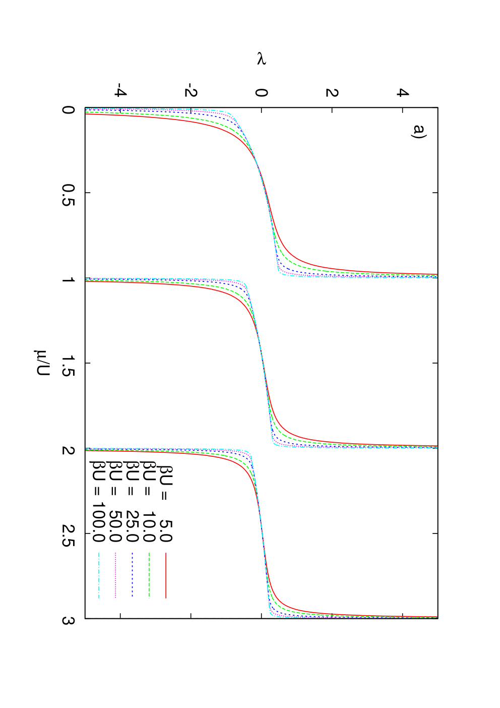
Explicit expressions for $\nu$ , $\lambda$ and $\kappa^{2}$ can be easily computed from Eqs. (35) and (36) and are given in Appendix C. The temperature and chemical potential dependence of these quantities is displayed in Figs. 2 a) - c). The phase boundary of the superfluid phase at finite temperature is shown for reference in Fig. 2 d). We can see that the strongest temperature dependence of the parameters is for values of $\mu/U$ close to an integer (which we ignore), and that both $\lambda$ and $\kappa^{2}$ are relatively insensitive to thermal effects over a wide range of $\mu/U$ values. The interaction term $u$ is most sensitive to temperature and starts to deviate strongly from its zero temperature value by temperatures as large as $T\simeq 0.2U$ , which corresponds to the temperature at which there is full melting of the insulating phase [28, 70].

Using a similar expansion to the one used to derive the mean field phase boundary, we can note that after a Fourier transform in space

	$\displaystyle 2J_{ij}(t)z_{jc}(t)$	$\displaystyle\to$	$\displaystyle 2J(t)\sum_{j=1}^{d}\cos(k_{j}a)\,z({\mathbf{k}},t)$		(23)
		$\displaystyle\simeq$	$\displaystyle 2J(t)\left[d-\frac{1}{2}k^{2}a^{2}\right]z({\mathbf{k}},t),$		(23)

for small $ka$ . We will focus on the long wavelength limit and ignore terms of order $ka$ .

We only retain the $k=0$ part of the interaction term, in keeping with our focus on long wavelength physics, and we take the low frequency limit of the interaction term by expanding the two particle connected Green’s function and the retarded and advanced Green’s functions about the $\omega=0$ limit. Recalling from above that $|z_{c}(t)|^{2}=2|z(t)|^{2}$ , we may approximate the interaction term by $-u|z|^{2}z$ , where $u$ is stated in Appendix C and is in accord with the static value calculated for equilibrium in Ref. [76]. Thus we have as our approximation to the equation of motion:

\left[2dJ(t)+\nu\right]z(t)-i\lambda\frac{\partial z(t)}{\partial t}-\kappa^{2}\frac{\partial^{2}z(t)}{\partial t^{2}}-u|z(t)|^{2}z(t)=0.

Take $J(t)=J_{0}+j(t)$ , where $J_{0}$ is chosen so that

2dJ_{0}+\nu=0,

i.e. $J_{0}$ is chosen to lie on the mean field phase boundary for the superfluid for a given $\mu$ . Hence we may write the approximate mean field equation of motion as

\displaystyle\kappa^{2}\frac{\partial^{2}z}{\partial t^{2}}+i\lambda\frac{\partial z}{\partial t}+\delta(t)z+u|z|^{2}z=0,

(24)

where $\delta(t)=-2dj(t)$ . Even after the simplifications made above, this equation for the dynamics of the order parameter is a non-linear second order differential equation, for which we are not able to find analytic solutions in general. Below we discuss numerical solutions of this equation, along with an analytic solution that can be determined in a special case which illuminates the properties of the solutions of the equation.

We study Eq. (24) for fixed $\mu$ and time-varying $J$ . In experiment, there is a confining potential so that there is a position dependent local chemical potential

\mu_{\rm local}(r)=\mu-V(r),

where $V(r)$ is the trapping potential. The solutions we obtain for the dynamics at fixed $\mu$ should be compared to the experimental situation in which one views the dynamics at fixed radius in a symmetric trap. (This picture should be reasonable at time scales shorter than the timescale for global mass redistribution in the trap, which can be quite long compared to microscopic timescales [94]).

If we fix $\mu$ , then there are two possibilities for the dynamics that we should consider: a) the particle-hole symmetric case, in which case $\lambda=0$ , and b) the generic case, in which $\lambda\neq 0$ . The particle-hole symmetric case corresponds to the transition at the tip of the Mott lobe as illustrated in Fig. 3.

We consider traversal of the quantum critical region as $\delta(t)$ varies with $t$ . We demand that

\lim_{t\to-\infty}\delta(t)=-\delta_{0};\quad{\rm and}\quad\lim_{t\to\infty}\delta(t)=\delta_{1}.

In our numerical solutions we use the form

\displaystyle\delta(t)=\left(\frac{\delta_{0}+\delta_{1}}{2}\right)\tanh\left(\frac{t}{\tau_{Q}}\right)+\frac{\delta_{1}-\delta_{0}}{2},

(25)

where, similarly to Cucchietti et al. [41], who studied the transition from Mott insulator to superfluid in the one dimensional BHM, we assume that there is a timescale $\tau_{Q}$ which is the characteristic time for $\delta(t)$ to cross from $-\delta_{0}$ to $\delta_{1}$ .

III.2 Particle-hole symmetric case

In the particle-hole symmetric case, $\lambda=0$ and the saddle point equation takes the form

\displaystyle\kappa^{2}\frac{\partial^{2}z}{\partial t^{2}}+\delta(t)z+u|z|^{2}z=0.

(26)

We can choose $z(t)=\rho(t)e^{i\theta(t)}$ , and then real and imaginary parts of the equation give

	$\displaystyle 0$	$\displaystyle=$	$\displaystyle\ddot{\rho}-\rho\left(\dot{\theta}\right)^{2}+\bar{\delta}\rho+u\rho^{3},$
	$\displaystyle 0$	$\displaystyle=$	$\displaystyle 2\dot{\theta}\dot{\rho}+\ddot{\theta}\rho$

where we rescaled

t=\kappa\bar{t};\quad\quad\bar{\delta}(\bar{t})=\delta(\kappa\bar{t})=\delta(t),

and wrote the equations in terms of the rescaled time co-ordinate $\bar{t}$ . The second equation can be integrated to give

\ln\left(\dot{\theta}\right)=-2\ln\rho+c_{1},

i.e. $\dot{\theta}\rho^{2}=c,$ so

\ddot{\rho}-\frac{c^{2}}{\rho^{3}}+\bar{\delta}\rho+u\rho^{3}=0.

The initial condition that the system is deep in the superfluid phase implies that as $t\to-\infty$ , $\dot{\theta}\to 0,$ and $\dot{\rho}\to 0$ , so $\rho=\sqrt{\frac{\delta_{0}}{u}},$ and $c=0$ (we choose $\theta=0$ without loss of generality). Thus

\ddot{\rho}+\bar{\delta}\rho+u\rho^{3}=0.

Rescaling $\rho\to\tilde{\rho}/\sqrt{u}$ , then dropping the tilde and bar,

\ddot{\rho}+\delta(t)\rho+\rho^{3}=0,

with $\rho\to\sqrt{\delta_{0}}$ as $t\to-\infty$ . In the long time limit, when $\delta(t)=\delta_{1}$ , then we may rewrite the differential equation for $\rho$ as

\frac{d}{dt}\left[\frac{1}{2}\left(\dot{\rho}\right)^{2}+\frac{\delta_{1}}{2}\rho^{2}+\frac{1}{4}\rho^{4}\right]=0,

Then

\dot{\rho}^{2}+\delta_{1}\rho^{2}+\frac{1}{2}\rho^{4}=A,

and, writing $\rho=\xi y$ , $t=\eta x$ , we have

\left(\frac{dy}{dx}\right)^{2}=(1-k^{2})-(1-2k^{2})y^{2}-k^{2}y^{4},

with

1-k^{2}=\frac{\eta^{2}A}{\xi^{3}},\quad k^{2}=\frac{1}{2}\xi^{2}\eta^{2},\quad 1-2k^{2}=\delta_{1}\eta^{2},

and we can solve to get

k=\frac{1}{\sqrt{2}}\frac{1}{\sqrt{1+\frac{\delta_{1}}{\xi^{2}}}},

which must satisfy $0<k<1$ . The solution to our equation as $t\to\infty$ is thus

\rho=\xi{\rm cn}\left(\frac{\xi t}{\sqrt{2}k};k\right),

which in the original variables is

z(t)=\frac{\xi}{\sqrt{u}}{\rm cn}\left(\frac{\xi}{\sqrt{2}k}\frac{t}{\kappa};k\right).

In general we cannot determine the value of $\xi$ analytically. We can obtain an analytical solution if there is a jump in $\delta(t)$ from $-\delta_{0}$ to $+\delta_{1}$ at $t=0$ . [Note that this form of $\delta(t)$ violates the assumption that we made in deriving the equation that frequencies are low, but the solution in this case is still instructive, as it shares many features with the solution for more physical forms of $\delta(t)$ .] We know $z(t)=\sqrt{\frac{\delta_{0}}{u}}$ for $t<0$ , and recalling ${\rm cn}(0;k)=1$ , we get $\xi=\sqrt{\delta_{0}}$ , which implies

k=\frac{1}{\sqrt{2}}\frac{1}{\sqrt{1+\frac{\delta_{1}}{\delta_{0}}}},

and so we get

\displaystyle z(t)=\sqrt{\frac{\delta_{0}}{u}}{\rm cn}\left(\frac{\sqrt{(\delta_{0}+\delta_{1})}t}{\kappa};\frac{1}{\sqrt{2}}\frac{1}{\sqrt{1+\frac{\delta_{1}}{\delta_{0}}}}\right),

which is periodic in time with average value 0 and period

4K\left(\frac{1}{\sqrt{2}}\frac{1}{\sqrt{1+\frac{\delta_{1}}{\delta_{0}}}}\right)\frac{\kappa}{\sqrt{\delta_{0}+\delta_{1}}}

where

K(k)=\int_{0}^{\frac{\pi}{2}}\frac{d\theta}{\sqrt{1-k^{2}\sin^{2}\theta}}.

We obtain numerical solutions of Eq. (26) with $\delta(t)$ taking the form given in Eq. (25) at the particle-hole symmetric point in the first Mott lobe for several different values of $\tau_{Q}$ , as displayed in Fig. 4. One can see that in each case, for large values of $t\gg\tau_{Q}$ , the form of the solution is that $z(t)$ oscillates in a periodic manner with a magnitude that decreases with increasing $\tau_{Q}$ . When averaged over a period $T$ at times $t\gg\tau_{Q}$ ,

\left<z\right>_{T}=\frac{1}{T}\int_{t}^{t+T}d\tilde{t}\,z(\tilde{t})=0,

as we would expect in the Mott insulating state. Defining $z_{\rm max}(\tau_{Q})=\lim_{t\to\infty}|z(t)|$ we can see that $z_{\rm max}(\tau_{Q})$ decreases with increasing $\tau_{Q}$ without any indication of saturation, as illustrated in the inset to Fig. 4. Note that in our numerical simulations $t$ is measured in units of $U^{-1}$ .

III.3 Generic case

In the generic case in which $\lambda\neq 0$ , we start with Eq. (24) and try for a solution of the form

z(t)=\rho(t)e^{i\theta(t)}.

Taking real and imaginary parts of the equation, after substitution gives

	$\displaystyle\kappa^{2}\left(\ddot{\rho}-\rho\left(\dot{\theta}\right)^{2}\right)-\lambda\rho\dot{\theta}+\delta(t)\rho+u\rho^{3}$	$\displaystyle=$	$\displaystyle 0,$
	$\displaystyle\kappa^{2}\left(2\dot{\theta}\dot{\rho}+\ddot{\theta}\rho\right)+\lambda\dot{\rho}$	$\displaystyle=$	$\displaystyle 0.$

Integrating the second equation with respect to $t$ leads to

\displaystyle\dot{\theta}=\frac{c-\frac{\lambda}{2}\rho^{2}}{\kappa^{2}\rho^{2}},

(27)

In the $t\to-\infty$ limit, $\rho$ and $\theta$ are constant, so we can determine $c=\frac{\lambda}{2}\rho_{0}^{2}=\frac{\lambda\delta_{0}}{2u},$ and we obtain the following equation for $\rho$ :

\displaystyle\kappa^{2}\ddot{\rho}-\frac{\lambda^{2}}{4\kappa^{2}\rho^{3}}\left(\frac{\delta_{0}}{u}\right)+\delta(t)\rho+u\rho^{3}=0.

(28)

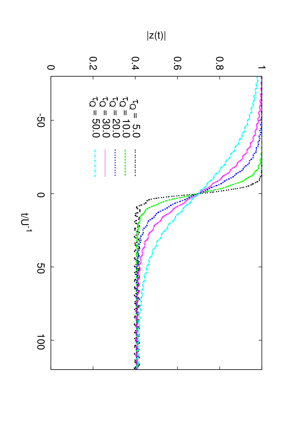
We solve Eq. (28) numerically for a variety of values of $\tau_{Q}$ and display $|z(t)|=\rho(t)$ for $\mu/U=0.25$ (well away from both degeneracy and the particle hole symmetric case) in Fig. 5.

The solution displays the similar feature to the particle-hole symmetric case that the average of $z$ over a period $\left<z\right>_{T}=0$ . However, it is clear that as $\tau_{Q}$ increases, there does not seem to be any decay in the values of $|z(t)|$ . By rescaling the time with $\tau_{Q}$ , we can see that in fact the different traces collapse onto each other, as we display in Fig. 6.

III.4 Chemical potential and temperature dependence of dynamics

The traces of $z(t)$ and $|z(t)|$ that we displayed in Figs. 4-6 were for a particular value of the chemical potential in the generic case and for a low temperature ( $\beta U=100$ ) in both cases. It is of interest to see whether the observation that in the non particle-hole symmetric case that there is a metastable state after a quantum quench is robust to variations of chemical potential and temperature. Defining $z_{\rm max}=\lim_{\tau_{Q}\to\infty}z_{\rm max}(\tau_{Q})$ , we calculated this for $0.1<\mu/U<0.9$ and temperatures ranging from $\beta U=100$ to $\beta U=2$ . We focus only on the first Mott lobe, but from perusal of the chemical potential and temperature dependence of the parameters $\lambda$ , $\kappa^{2}$ and $u$ in Fig. 2, we expect that similar qualitative results should be obtained for other Mott lobes. We find that apart from the particle-hole symmetric point, where we believe the displayed finite value of $z_{\rm max}$ is an artefact of our numerical calculations, that the transition to a metastable state in which $z_{\rm max}\neq 0$ is generic for a wide range of values of $\mu$ and persists to temperatures comparable to the melting temperature of the insulator as illustrated in Fig. 7. It should be noted that the physics that we have left out of dynamical equation, namely spatial dependence of $z$ and also higher frequency components of $z$ will presumably lead to equilibration of $z$ at long enough times, but as we argue in Sec. IV, it may well be reasonable to expect that the behaviour we identify at the mean field level to be experimentally relevant on appropriate timescales.

IV Discussion and Conclusions

In this paper we have derived a real time effective action for the Bose Hubbard model using the Schwinger-Keldysh technique, generalizing previous work that obtained an equilibrium effective action [76]. This action allows for a description of the properties of both the superfluid and Mott insulating phases. Hence we are able to study the out of equilibrium dynamics as the parameters in the Hamiltonian are changed so that the ground state is tuned from one phase to another. We obtain the saddle point equations of motion and by focusing on low frequency, long wavelength dynamics are able to obtain an equation of motion for the superfluid order parameter. We have focused on this case as the simplest example of dynamics, but we emphasise that our approach leads to equations of motion that can be used to study high frequencies and spatial variations of the order parameter and its correlations.

We study the equations of motion by varying the hopping parameter $J$ as a function of time at fixed chemical potential to sweep from deep in the superfluid phase to deep in the Mott insulating phase over a timescale of order $\tau_{Q}$ . We study the $\tau_{Q}$ dependence of the superfluid order parameter numerically and find that in the long $\tau_{Q}$ limit the system generically reaches a state in which the time averaged value of the order parameter is zero (as would be expected in equilibrium for a Mott insulator), but the absolute value of the order parameter is non-zero. The magnitude of the order parameter in the long $\tau_{Q}$ limit appears to vanish only at the particle-hole symmetric value of the chemical potential, and grows with distance from the particle-hole symmetric value of $\mu$ . The generic final state is clearly an out-of-equilibrium metastable state, with equilibration only possibly for the particle-hole symmetric case. The generically non-zero value of $|z(t)|$ in the final state indicates that the system retains memory of the initial superfluid state, a feature which is observed in quantum revival experiments [99, 100, 101] that indicate quantum coherence remains even after a quench into the insulating phase.

There have been several other recent theoretical works on the out-of-equilibrium dynamics of the Bose Hubbard model that see evidence of the system entering a metastable state after a sweep from the superfluid phase to the Mott insulating state. Schützhold et al. [40] studied the dynamics in the limit of large number of bosons per site and found a slow decay of the superfluid fraction for a slow sweep from the superfluid phase to the Mott insulating phase. Kollath et al. [42] investigated the one and two dimensional BHM numerically with the number of bosons fixed to an average of one boson per site and found that for small enough values of the final value of the hopping, the system reached a non-thermal steady state which was relatively insensitive to the details of the initial state. These authors determined whether the system was thermal or not by investigating real-space correlations, so it is not possible to make a direct comparison with our results here. Most recently Sciolla and Biroli [13] considered the infinite dimensional Bose Hubbard model at integer filling and also found that the final state after a quantum quench of $U$ showed a non-zero superfluid order parameter. Similar features have also been reported for mean field studies of fermions after a quantum quench [102].

Whilst the emergence of a metastable state after a quench from the superfluid to the insulating state is also seen in our work, we study a different situation to the previous works. We consider a spatially uniform BHM, as do Refs. [40, 42, 13], but we consider fixed chemical potential rather than fixed particle number. To compare theoretical descriptions of the out of equilibrium dynamics of the Bose Hubbard model and experiments on the quench dynamics of a fixed number of cold atoms in an optical lattice, the physical meaning of working with fixed chemical potential needs to be discussed. The presence of a spatially non-uniform trapping potential means that instead of viewing the system as having a uniform chemical potential, it is often more convenient to view the system as having a spatially dependent local chemical potential: $\mu_{\rm local}({\mathbf{r}})=\mu-V({\mathbf{r}})$ , where $V({\mathbf{r}})$ is the trapping potential. For a symmetric trap, this implies that a reasonable description of the phase the system is in at radius $r$ can be determined by using $\mu_{\rm local}(r)$ – this implies the “wedding cake” structure seen in many experiments. Our study of the equations of motion at fixed chemical potential would then correspond to studying the dynamics of atoms in a trap at fixed radius (albeit with radii corresponding to certain values of the chemical potential excluded due to the approximations we made in deriving the equation of motion).

This viewpoint appears to be borne out in recent experiments [34, 103, 104, 33] and theoretical work [94, 105] on quantum quenches for cold bosons. Natu et al. [94] argue that the very large differences in relaxation times observed in Refs. [34] (of order ms) and [103] (of order $\sim$ 1s) can be understood if one looks at mass transport during equilibration. If the average number of particles per site remains the same in crossing from the superfluid to an insulator, then equilibration can be quick as in Ref. [34], but if the average number of particles per site needs to change, then there must be mass transport and the equilibration is slow as in Ref. [103]. The results we find for the long time limit of $z_{\rm max}$ illustrated in Fig. 7 are in accord with this idea. For the chemical potential associated with particle hole symmetry, the value of $z_{\rm max}$ decays to (close to) zero, whereas for other values of $\mu$ , $z_{\rm max}$ can be an appreciable fraction of the value of $|z|$ in the initial state. At the particle hole symmetric $\mu$ , the average number of bosons per site does not change in crossing from the superfluid to the Mott insulator [20], in accord with the condition for local equilibration without mass transport [94]. Global mass transport is not captured within our simplified equation of motion, and there is no decay of the metastable state and equilibration on a longer time scales.

The main results of our work and their connection to existing experimental and theoretical work in the field of cold atoms are outlined above, but there are a number of future directions that it might be interesting to pursue based on what we have done here. First, a more thorough study of the solutions of the equations of motion allowing for spatial fluctuations and higher frequencies than we consider here might lead to further insight into the dynamics of the Bose Hubbard model. The inclusion of a trapping potential would also allow for additional contact with experiment [106]. Second, it would be interesting to add the effects of dissipation [107, 55], which has been shown to renormalize the phase boundaries in the BHM. For cold atoms the effects of dissipation can probably be ignored, but in other realizations of the BHM this may not be feasible [108].

Recent experimental advances which allow for high spatial resolution in cold atom experiments [109, 110, 104, 111, 34, 112] suggests that there will be advanced capabilities for probing the out of equilibrium dynamics spatially as well as temporally, suggesting that there are exciting times ahead for studies of out of equilibrium dynamics of Bose Hubbard systems.

V Acknowledgements

The authors thank Claudio Chamon for helpful discussions and encouragement, especially in the early stages of this work and Jeff McGuirk for a critical reading of the manuscript. This work was supported by NSERC.

Appendix A Hubbard-Stratonovich transformation

Starting from the identities (where $z=x+iy$ )

\int_{-\infty}^{\infty}\int_{-\infty}^{\infty}\frac{dxdy}{i\pi}e^{i|z|^{2}}=\int_{-\infty}^{\infty}\int_{-\infty}^{\infty}\frac{dxdy}{(-i\pi)}e^{-i|z|^{2}}=1,

it is easy to show that

e^{-ia^{*}a}=\int_{-\infty}^{\infty}\int_{-\infty}^{\infty}\frac{dxdy}{i\pi}e^{i|z|^{2}+i(z^{*}a+za^{*})};\quad e^{ia^{*}a}=\int_{-\infty}^{\infty}\int_{-\infty}^{\infty}\frac{dxdy}{(-i\pi)}e^{-i|z|^{2}+i(z^{*}a+za^{*})}.

Using these results we may write (with $z_{1}=x_{1}+iy_{1}$ , $z_{2}=x_{2}+iy_{2}$ and $z_{3}=x_{3}+iy_{3}$ )

$\displaystyle e^{-i(\xi^{}\eta+\eta^{}\xi)}$	$\displaystyle=$	$\displaystyle e^{-i(\xi^{}+\eta^{})(\xi+\eta)+i\xi^{}\xi+i\eta^{}\eta}$
	$\displaystyle=$	$\displaystyle\int\frac{dx_{1}dy_{1}}{i\pi}\int\frac{dx_{2}dy_{2}}{(-i\pi)}\int\frac{dx_{3}dy_{3}}{(-i\pi)}e^{i\|z_{1}\|^{2}-i\|z_{2}\|^{2}-i\|z_{3}\|^{2}}e^{i\left(z_{1}(\xi^{}+\eta^{})+z_{1}^{}(\xi+\eta)+z_{2}\xi^{}+z_{2}^{}\xi+z_{3}\eta^{}+z_{3}^{*}\eta\right)}$
	$\displaystyle=$	$\displaystyle\int\frac{d\tilde{x}_{1}d\tilde{y}_{1}}{i\pi}\frac{d\tilde{x}_{2}d\tilde{y}_{2}}{(-i\pi)}\frac{d\tilde{x}_{3}d\tilde{y}_{3}}{(-i\pi)}e^{i\|\tilde{z}_{1}\|^{2}-i\|\tilde{z}_{2}-\tilde{z}_{1}\|^{2}-i\|\tilde{z}_{3}-\tilde{z}_{1}\|^{2}}e^{i\left(\tilde{z}_{2}^{}\xi+\tilde{z}_{2}\xi^{}+\tilde{z}_{3}^{}\eta+\tilde{z}_{3}\eta^{}\right)}$

where we change variables to $\tilde{z}_{1}=z_{1}$ , $\tilde{z_{2}}=z_{1}+z_{2}$ , and $\tilde{z}_{3}=z_{1}+z_{3}$ . After integrating out $\tilde{z}_{1}$ , we get

	$\displaystyle e^{-i(\xi^{}\eta+\xi\eta^{})}$	$\displaystyle=$	$\displaystyle\int\frac{d\tilde{x}_{2}d\tilde{y}_{2}}{(-i\pi)}\frac{d\tilde{x}_{3}d\tilde{y}_{3}}{i\pi}e^{2i(\tilde{x}_{2}\tilde{x}_{3}+\tilde{y_{2}}\tilde{y}_{3})}e^{i(\tilde{z}_{2}^{}\xi+\tilde{z}_{2}\xi^{}+\tilde{z}_{3}\eta^{}+\tilde{z}_{3}^{}\eta)}$		(29)
		$\displaystyle=$	$\displaystyle\int\overline{\mathcal{D}}(z_{2},z_{2}^{}){\mathcal{D}}(z_{3},z_{3}^{})e^{i(z_{2}^{}z_{3}+z_{2}z_{3}^{})}e^{i(z_{2}^{}\xi+z_{2}\xi^{}+z_{3}\eta^{*}+z_{3}\eta)},$		(29)

where

{\mathcal{D}}(z,z^{*})=\frac{dxdy}{i\pi};\quad\quad\overline{\mathcal{D}}(z,z^{*})=\frac{dxdy}{(-i\pi)}.

Appendix B Mean field phase boundary

One way to determine the mean field phase boundary between the superfluid and Mott insulating phases is to determine when the coefficient of the quadratic term in the action Eq. () vanishes. In order to do this it is helpful to note that

\displaystyle\tau^{1}_{a_{1}b_{1}}G_{ib_{1}b_{2}}(t_{1},t_{2})\tau^{1}_{b_{2}a_{2}}=\left(\begin{array}[]{cc}{\mathcal{G}}_{0}^{K}(t_{1},t_{2})&{\mathcal{G}}_{0}^{R}(t_{1},t_{2})\\ {\mathcal{G}}_{0}^{A}(t_{1},t_{2})&0\end{array}\right),

where ${\mathcal{G}}_{0}^{R}$ , ${\mathcal{G}}_{0}^{A}$ , and ${\mathcal{G}}_{0}^{K}$ are the retarded, advanced and Keldysh propagators respectively, with the subscript $0$ indicating that these are the propagators associated with $H_{0}$ . The definitions of the propagators are:

$\displaystyle i{\mathcal{G}}_{0}^{K}(t-t^{\prime})$	$\displaystyle=$	$\displaystyle i{\mathcal{G}}_{0}^{<}(t,t^{\prime})+i{\mathcal{G}}_{0}^{>}(t,t^{\prime}),$
$\displaystyle i{\mathcal{G}}_{0}^{R}(t-t^{\prime})$	$\displaystyle=$	$\displaystyle\theta(t-t^{\prime})[i{\mathcal{G}}_{0}^{>}(t,t^{\prime})-i{\mathcal{G}}_{0}^{<}(t,t^{\prime})],$
$\displaystyle i{\mathcal{G}}_{0}^{A}(t-t^{\prime})$	$\displaystyle=$	$\displaystyle\theta(t^{\prime}-t)[i{\mathcal{G}}_{0}^{<}(t,t^{\prime})-i{\mathcal{G}}_{0}^{>}(t,t^{\prime})],$

with

	$\displaystyle i{\mathcal{G}}_{0}^{<}(t,t^{\prime})$	$\displaystyle=$	$\displaystyle\frac{{\rm Tr}\{\hat{a}^{\dagger}(t^{\prime})\hat{a}(t)\hat{\rho}_{0}\}}{Z},$
	$\displaystyle i{\mathcal{G}}_{0}^{>}(t,t^{\prime})$	$\displaystyle=$	$\displaystyle\frac{{\rm Tr}\{\hat{a}(t)\hat{a}^{\dagger}(t^{\prime})\hat{\rho}_{0}\}}{Z}.$

These expressions can be evaluated using the interaction representation

	$\displaystyle\hat{a}^{\dagger}(t^{\prime})$	$\displaystyle=$	$\displaystyle e^{i(\hat{H}_{U}-\mu\hat{n})t^{\prime}}\hat{a}^{\dagger}e^{-i(\hat{H}_{U}-\mu\hat{n})t^{\prime}}$
	$\displaystyle\hat{a}(t)$	$\displaystyle=$	$\displaystyle e^{i(\hat{H}_{U}-\mu\hat{n})t}\hat{a}e^{-i(\hat{H}_{U}-\mu\hat{n})t}$

we obtain

\displaystyle i{\mathcal{G}}_{0}^{<}(t,t^{\prime})

\displaystyle=

\displaystyle re^{-i(E_{r}-\mu r)t}e^{i(E_{r-1}-\mu(r-1))(t-t^{\prime})}e^{i(E_{r}-\mu r)t^{\prime}},

where we recalled $\hat{a}\left|r\right>=\sqrt{r}\left|r-1\right>$ and $\hat{a}^{\dagger}\left|r\right>=\sqrt{r+1}\left|r+1\right>$ . At temperature $T$ ,

\displaystyle i{\mathcal{G}}_{0}^{<}(t,t^{\prime})

\displaystyle=

\displaystyle\frac{\sum_{r=0}^{\infty}re^{i(\mu-U(r-1))(t-t^{\prime})}e^{-\beta(E_{r}-\mu r)}}{\sum_{r=0}^{\infty}e^{-\beta(E_{r}-\mu r)}}.

Hence we have that the retarded Green’s function takes the form

\displaystyle{\mathcal{G}}_{0}^{R}(t_{1},t_{2})=-i\theta(t_{1}-t_{2})\frac{1}{\sum_{r=0}^{\infty}e^{-\frac{1}{T}(E_{r}-\mu r)}}\left\{\sum_{r=0}^{\infty}\left[(r+1)e^{i(\mu-Ur)(t_{1}-t_{2})}-re^{i(\mu-U(r-1))(t_{1}-t_{2})}\right]e^{-\frac{(E_{r}-\mu r)}{T}}\right\},

(35)

which simplifies at $T=0$ to

\displaystyle{\mathcal{G}}_{0}^{R}(t_{1},t_{2})=-i\theta(t_{1}-t_{2})\left[(n_{0}+1)e^{i(\mu-Un_{0})(t_{1}-t_{2})}-n_{0}e^{i(\mu-U(n_{0}-1))(t_{1}-t_{2})}\right].

(36)

For future reference it will also be convenient to note that

\displaystyle{\mathcal{G}}_{0}^{K}(t_{1},t_{2})=-\frac{i}{\sum_{r=0}^{\infty}e^{-\beta(E_{r}-\mu r)}}\sum_{r=0}^{\infty}e^{-\beta(E_{r}-\mu r)}\left[(r+1)e^{i(\mu-Ur)(t_{1}-t_{2})}+re^{i(\mu-U(r-1))(t_{1}-t_{2})}\right],

(37)

which simplifies at $T=0$ to

{\mathcal{G}}_{0}^{K}(t_{1},t_{2})=-i\left[(n_{0}+1)e^{i(\mu-Un_{0})(t_{1}-t_{2})}+n_{0}e^{i(\mu-U(n_{0}-1))(t_{1}-t_{2})}\right].

Recalling that we can treat this as a single site problem we have

{\hat{\rho}}_{0}=e^{-\beta\left[\frac{U}{2}(\hat{n}(\hat{n}-1)-\mu\hat{n})\right]};\quad Z={\rm Tr}\{\hat{\rho}_{0}\}=\sum_{r=0}^{\infty}e^{-\beta(E_{r}-\mu r)},

and $E_{r}=\frac{U}{2}r(r-1)$ . $n=N/M$ , where $N$ is the number of bosons and $M$ the number of sitesa $\mu$ is determined implicitly from

n=\frac{\sum_{r=0}^{\infty}re^{-\beta(E_{r}-\mu r)}}{\sum_{r=0}^{\infty}e^{-\beta(E_{r}-\mu r)}}.

At $T=0$ , the value of $\mu/U$ sets the occupation number, $n_{0}\left(\frac{\mu}{U}\right)$ which takes an integer value $r$ for $r-1<\mu/U<r$ , with degeneracies at $\mu/U=0,1,2,\ldots$ .

When we Fourier transform the quadratic part of $S_{\rm eff}^{I}$ in space and time we get:

\displaystyle-\int_{-\infty}^{\infty}\frac{d\omega}{2\pi}\sum_{k}\frac{1}{J_{{\mathbf{k}}}}\psi_{a}^{*}(\omega,{\mathbf{k}})\tau^{1}_{ab}\psi_{b}(\omega,{\mathbf{k}})-\int\frac{d\omega}{2\pi}\sum_{{\mathbf{k}}}\psi_{a_{1}}^{*}(\omega,{\mathbf{k}})\tau^{1}_{a_{1}b_{1}}G_{b_{1}b_{2}}(\omega)\tau^{1}_{b_{2}a_{2}}\psi_{a_{2}}(\omega,{\mathbf{k}}).

(38)

We choose the hopping amplitude $J_{ij}$ to take the form

J_{ij}(t)=\left\{\begin{array}[]{cc}J_{0}+j(t),&i,j\,{\rm nearest\,neighbours}\\ 0,&{\rm otherwise}\end{array}\right.,

for which (with $a$ the lattice spacing)

	$\displaystyle J_{{\mathbf{k}}}(t)$	$\displaystyle=$	$\displaystyle\left[J_{0}+j(t)\right]\sum_{j=1}^{d}\cos(k_{j}a)$
		$\displaystyle\simeq$	$\displaystyle\left(d-\frac{1}{2}k^{2}a^{2}\right)\left[J_{0}+j(t)\right],$

assuming that $ka\ll 1$ .

Setting $j(t)=0$ for now, when we take the $\omega$ , $k$ $\to$ 0 limit we can locate the phase boundary by noting when the coefficient of the $\psi_{q}^{*}\psi_{c}$ term in the action vanishes:

\frac{1}{2dJ_{0}}+{\mathcal{G}}_{0}^{R}(\omega=0)=0.

Note that the retarded propagator

\displaystyle{\mathcal{G}}^{R}_{0}(\omega)=\frac{1}{\sum_{r=0}^{\infty}e^{-\frac{1}{T}(E_{r}-\mu r)}}\sum_{r=0}^{\infty}e^{-\frac{(E_{r}-\mu r)}{T}}\left[\frac{(r+1)}{\mu-Ur+\omega+i0}-\frac{r}{\mu-U(r-1)+\omega+i0}\right],

(39)

at finite $T$ and for $T=0$

\displaystyle{\mathcal{G}}_{0}^{R}(\omega)=\frac{n_{0}+1}{\mu-Un_{0}+\omega+i0}-\frac{n_{0}}{\mu-U(n_{0}-1)+\omega+i0}.

The advanced propagator may be obtained from

{\mathcal{G}}_{0}^{A}(\omega)=\left[{\mathcal{G}}_{0}^{R}(\omega)\right]^{*},

and at $T=0$ the Keldysh propagator is

	$\displaystyle{\mathcal{G}}_{0}^{K}(\omega)$	$\displaystyle=$	$\displaystyle-2i\pi\left[(n_{0}+1)\delta(\omega+\mu-Un_{0})\right.$		(41)
			$\displaystyle\left.+n_{0}\delta(\omega+\mu-U(n_{0}-1))\right]$		(41)

At zero temperature we obtain the standard mean field equation for the phase boundary between the Mott insulator and superfluid phases:

\frac{1}{2dJ_{0}}+\frac{(n_{0}+1)}{\mu-Un_{0}}-\frac{n_{0}}{\mu-U(n_{0}-1)}=0.

This may also be expressed as

\displaystyle\tilde{\mu}_{\pm}=\frac{1}{2}\left[(2n_{0}+1)-\tilde{J}\pm\sqrt{1-\tilde{J}(2n_{0}+1)+\tilde{J}^{2}}\right],

for $n_{0}>1$ and $\tilde{\mu}_{+}=-\tilde{J}$ if $n_{0}=0$ , where $\tilde{J}=2dJ/U$ and $\tilde{\mu}=\mu/U$ . This affirms that the effective action correctly predicts the mean field phase boundary at zero temperature. At finite temperature the corresponding equation is

	$\displaystyle\frac{1}{2dJ_{0}}+\frac{1}{Z}\sum_{r=0}^{\infty}e^{-\beta(E_{r}-\mu r)}\left[\frac{r+1}{\mu-Ur}-\frac{r}{\mu-U(r-1)}\right]=0.$
			(43)

The phase boundary as determined from this equation for a variety of $\beta$ values is displayed in Fig. 2 d). This phase boundary is the edge of the superfluid phase – the Mott insulator is strictly defined only at $T=0$ , and at non-zero temperature there can be a normal phase separating superfluid and insulator, with full melting of the insulator for $T^{*}\simeq 0.2\,U$ [28, 70].

Appendix C Parameters in the equation of motion

There are three parameters that enter the equation of motion:

\nu=\left[{\mathcal{G}}_{0}^{R}\right]^{-1}_{\omega=0};\lambda=-\left.\frac{\partial}{\partial\omega}\left[{\mathcal{G}}_{0}^{R}\right]^{-1}\right|_{\omega=0};\kappa^{2}=\left.\frac{1}{2}\frac{\partial^{2}}{\partial\omega^{2}}\left[{\mathcal{G}}_{0}^{R}\right]^{-1}\right|_{\omega=0}.

These can be evaluated to give

\displaystyle\nu=\frac{Z}{\sum_{r=0}^{\infty}e^{-\beta(E_{r}-\mu r)}\left[\frac{(r+1)}{\mu-Ur}-\frac{r}{\mu-U(r-1)}\right]},

(44)

\displaystyle\lambda=\frac{\nu^{2}}{Z}\sum_{r=0}^{\infty}e^{-\beta(E_{r}-\mu r)}\left[\frac{(r+1)}{[\mu-Ur]^{2}}-\frac{r}{[\mu-U(r-1)]^{2}}\right],

(45)

\displaystyle\kappa^{2}

\displaystyle=

\displaystyle\frac{\lambda^{2}}{\nu}-\frac{\nu^{2}}{Z}\sum_{r=0}^{\infty}e^{-\beta(E_{r}-\mu r)}\left[\frac{(r+1)}{[\mu-Ur]^{3}}-\frac{r}{[\mu-U(r-1)]^{3}}\right],

(46)

and

	$\displaystyle u$	$\displaystyle=$	$\displaystyle-\frac{\nu^{4}}{2Z}\sum_{r=0}^{\infty}e^{-\beta(E_{r}-\mu_{r})}\left\{\frac{4(p+1)(p+2)}{[Up-\mu]^{2}[2\mu-(2p+1)U]}+\frac{4p(p-1)}{[U(p-1)-\mu]^{2}[U(2p-3)-2\mu]}-\frac{4(p+1)^{2}}{[\mu-Up]^{3}}\right.$		(47)
			$\displaystyle\hskip 99.58464pt\left.-\frac{4p^{2}}{[U(p-1)-\mu]^{3}}-\frac{4p(p+1)}{[U(p-1)-\mu]^{2}[\mu-Up]}-\frac{4p(p+1)}{[U(p-1)-\mu][\mu-Up]^{2}}\right\}.$		(47)

The expressions for $\nu$ , $\lambda$ and $\kappa^{2}$ simplify somewhat in the zero temperature limit:

\nu=\frac{(\mu-Un_{0})(\mu-U(n_{0}-1))}{\mu+U};\quad\quad\lambda=\frac{(2n_{0}-1)U-2\mu}{\mu+U}+\frac{(\mu-Un_{0})(\mu-U(n_{0}-1))}{(\mu+U)^{2}}

and

\displaystyle\kappa^{2}=\frac{1}{2}\left[\frac{2n_{0}U-\mu}{(\mu+U)^{2}}-\left\{\frac{(U\mu(2n_{0}+1)-U^{2}(2n_{0}^{2}-1)}{(\mu+U)^{3}}\right\}\right].

(48)

Appendix D Evaluation of the four point function

To evaluate the four time correlation functions, there are several basic correlations we need:

$\displaystyle B^{aaa^{\dagger}a^{\dagger}}(t_{1},t_{2},t_{3},t_{4})$	$\displaystyle=$	$\displaystyle\frac{1}{Z}{\rm Tr}\left\{e^{-\beta(\hat{H}_{U}-\mu\hat{N})}a(t_{1})a(t_{2})a^{\dagger}(t_{3})a^{\dagger}(t_{4})\right\}$	(49)
	$\displaystyle=$	$\displaystyle\frac{1}{Z}\sum_{p=0}^{\infty}(p+1)(p+2)e^{i(E_{p}-\mu p)(t_{1}-t_{4}+i\beta)+i(E_{p+1}-\mu(p+1))(t_{2}+t_{4}-t_{1}-t_{3})+i(E_{p+2}-\mu(p+2))(t_{3}-t_{2})},$	(49)
$\displaystyle B^{aa^{\dagger}aa^{\dagger}}(t_{1},t_{2},t_{3},t_{4})$	$\displaystyle=$	$\displaystyle\frac{1}{Z}\sum_{p=0}^{\infty}(p+1)^{2}e^{i(E_{p}-\mu p)(t_{1}+t_{3}-t_{2}-t_{4}+i\beta)+i(E_{p+1}-\mu(p+1))(t_{2}+t_{4}-t_{1}-t_{3})},$	(50)
$\displaystyle B^{aa^{\dagger}a^{\dagger}a}(t_{1},t_{2},t_{3},t_{4})$	$\displaystyle=$	$\displaystyle\frac{1}{Z}\sum_{p=0}^{\infty}p(p+1)e^{i(E_{p}-\mu p)(t_{1}+t_{3}-t_{2}-t_{4}+i\beta)+i(E_{p-1}-\mu(p-1))(t_{4}-t_{3})+i(E_{p+1}-\mu(p+1))(t_{2}-t_{1})},$	(51)
$\displaystyle B^{a^{\dagger}aaa^{\dagger}}(t_{1},t_{2},t_{3},t_{4})$	$\displaystyle=$	$\displaystyle\frac{1}{Z}\sum_{p=0}^{\infty}p(p+1)e^{i(E_{p}-\mu p)(t_{1}+t_{3}-t_{2}-t_{4}+i\beta)+i(E_{p+1}-\mu(p+1))(t_{4}-t_{3})+i(E_{p-1}-\mu(p-1))(t_{2}-t_{1})},$	(52)
$\displaystyle B^{a^{\dagger}aa^{\dagger}a}(t_{1},t_{2},t_{3},t_{4})$	$\displaystyle=$	$\displaystyle\frac{1}{Z}\sum_{p=0}^{\infty}p^{2}e^{i(E_{p}-\mu p)(t_{1}+t_{3}-t_{2}-t_{4}+i\beta)+i(E_{p-1}-\mu(p-1))(t_{2}+t_{4}-t_{1}-t_{3})},$	(53)
$\displaystyle B^{a^{\dagger}a^{\dagger}aa}(t_{1},t_{2},t_{3},t_{4})$	$\displaystyle=$	$\displaystyle\frac{1}{Z}\sum_{p=0}^{\infty}p(p-1)e^{i(E_{p}-\mu p)(t_{1}-t_{4}+i\beta)+i(E_{p-1}-\mu(p-1))(t_{2}+t_{4}-t_{1}-t_{3})+i(E_{p-2}-\mu(p-2))(t_{3}-t_{2})}.$	(54)

In addition we require the two point correlations

$\displaystyle C^{aa^{\dagger}}(t_{1},t_{2})$	$\displaystyle=$	$\displaystyle\frac{1}{Z}{\rm Tr}\left\{e^{-\beta(\hat{H}_{U}-\mu\hat{N})}a(t_{1})a^{\dagger}(t_{2})\right\}$	(55)
	$\displaystyle=$	$\displaystyle\frac{1}{Z}\sum_{p=0}^{\infty}(p+1)e^{i(E_{p}-\mu p)(t_{1}-t_{2}+i\beta)+i(E_{p+1}-\mu(p+1))(t_{2}-t_{1})}$
	$\displaystyle=$	$\displaystyle i{\mathcal{G}}_{0}^{>}(t_{1},t_{2}),$
$\displaystyle C^{a^{\dagger}a}(t_{1},t_{2})$	$\displaystyle=$	$\displaystyle\frac{1}{Z}\sum_{p=0}^{\infty}pe^{i(E_{p}-\mu p)(t_{1}-t_{2}+i\beta)+i(E_{p-1}-\mu(p-1))(t_{2}-t_{1})}$	(56)
	$\displaystyle=$	$\displaystyle i{\mathcal{G}}_{0}^{<}(t_{2},t_{1}).$	(56)

The actual expressions are rather tiresome to derive but are given here for completeness, where we use the notation $\theta_{ij}=\theta(t_{i}-t_{j})$ :

$\displaystyle G^{2c}_{qqqq}(t_{1},t_{2},t_{3},t_{4})$	$\displaystyle=$	$\displaystyle\frac{i}{2}\left\{\left[\theta_{12}\theta_{23}+\theta_{21}\theta_{14}\right]\left(B^{a^{\dagger}aaa^{\dagger}}(t_{3},t_{2},t_{1},t_{4})+B^{a^{\dagger}aaa^{\dagger}}(t_{4},t_{1},t_{2},t_{3})\right)\right.$	(57)
		$\displaystyle+\left[\theta_{12}\theta_{24}+\theta_{21}\theta_{13}\right]\left(B^{a^{\dagger}aaa^{\dagger}}(t_{3},t_{1},t_{2},t_{4})+B^{a^{\dagger}aaa^{\dagger}}(t_{4},t_{2},t_{1},t_{3})\right)$
		$\displaystyle+\left[\theta_{13}\theta_{32}+\theta_{31}\theta_{14}\right]\left(B^{aa^{\dagger}aa^{\dagger}}(t_{2},t_{3},t_{1},t_{4})+B^{a^{\dagger}aa^{\dagger}a}(t_{4},t_{1},t_{3},t_{2})\right)$
		$\displaystyle+\left[\theta_{13}\theta_{34}+\theta_{31}\theta_{12}\right]\left(B^{aaa^{\dagger}a^{\dagger}}(t_{2},t_{1},t_{3},t_{4})+B^{a^{\dagger}aaa^{\dagger}}(t_{4},t_{3},t_{1},t_{2})\right)$
		$\displaystyle+\left[\theta_{14}\theta_{42}+\theta_{41}\theta_{13}\right]\left(B^{aa^{\dagger}aa^{\dagger}}(t_{2},t_{4},t_{1},t_{3})+B^{a^{\dagger}aa^{\dagger}a}(t_{3},t_{1},t_{4},t_{2})\right)$
		$\displaystyle+\left[\theta_{14}\theta_{43}+\theta_{41}\theta_{12}\right]\left(B^{aaa^{\dagger}a^{\dagger}}(t_{2},t_{1},t_{4},t_{3})+B^{a^{\dagger}a^{\dagger}aa}(t_{3},t_{4},t_{1},t_{2})\right)$
		$\displaystyle+\left[\theta_{32}\theta_{21}+\theta_{23}\theta_{34}\right]\left(B^{aaa^{\dagger}a^{\dagger}}(t_{1},t_{2},t_{3},t_{4})+B^{a^{\dagger}a^{\dagger}aa}(t_{4},t_{3},t_{2},t_{1})\right)$
		$\displaystyle+\left[\theta_{42}\theta_{21}+\theta_{24}\theta_{43}\right]\left(B^{aaa^{\dagger}a^{\dagger}}(t_{1},t_{2},t_{4},t_{3})+B^{a^{\dagger}a^{\dagger}aa}(t_{3},t_{4},t_{2},t_{1})\right)$
		$\displaystyle+\left[\theta_{23}\theta_{31}+\theta_{32}\theta_{24}\right]\left(B^{aa^{\dagger}aa^{\dagger}}(t_{1},t_{3},t_{2},t_{4})+B^{a^{\dagger}aa^{\dagger}a}(t_{4},t_{2},t_{3},t_{1})\right)$
		$\displaystyle+\left[\theta_{43}\theta_{31}+\theta_{34}\theta_{42}\right]\left(B^{aa^{\dagger}a^{\dagger}a}(t_{1},t_{3},t_{4},t_{2})+B^{aa^{\dagger}a^{\dagger}a}(t_{2},t_{4},t_{3},t_{1})\right)$
		$\displaystyle+\left[\theta_{24}\theta_{41}+\theta_{42}\theta_{23}\right]\left(B^{aa^{\dagger}aa^{\dagger}}(t_{1},t_{4},t_{2},t_{3})+B^{a^{\dagger}aa^{\dagger}a}(t_{3},t_{2},t_{4},t_{1})\right)$
		$\displaystyle\left.+\left[\theta_{34}\theta_{41}+\theta_{43}\theta_{32}\right]\left(B^{aa^{\dagger}a^{\dagger}a}(t_{1},t_{4},t_{3},t_{2})+B^{aa^{\dagger}a^{\dagger}a}(t_{2},t_{3},t_{4},t_{1})\right)\right\}$
		$\displaystyle-i\left\{\left[C^{aa^{\dagger}}(t_{1},t_{3})+C^{a^{\dagger}a}(t_{3},t_{1})\right]\left[C^{aa^{\dagger}}(t_{2},t_{4})+C^{a^{\dagger}a}(t_{4},t_{2})\right]\right.$
		$\displaystyle\left.+\left[C^{aa^{\dagger}}(t_{1},t_{4})+C^{a^{\dagger}a}(t_{4},t_{1})\right]\left[C^{aa^{\dagger}}(t_{2},t_{3})+C^{a^{\dagger}a}(t_{3},t_{2})\right]\right\},$

$\displaystyle G^{2c}_{cqqq}(t_{1},t_{2},t_{3},t_{4})$	$\displaystyle=$	$\displaystyle\frac{i}{2}\left\{-\theta_{21}\left[\theta_{32}+\theta_{23}\theta_{34}\right]\left(B^{aaa^{\dagger}a^{\dagger}}(t_{1},t_{2},t_{3},t_{4})-B^{a^{\dagger}a^{\dagger}aa}(t_{4},t_{3},t_{2},t_{1})\right)\right.$	(58)
		$\displaystyle-\theta_{21}\left[\theta_{42}+\theta_{24}\theta_{43}\right]\left(B^{aaa^{\dagger}a^{\dagger}}(t_{1},t_{2},t_{4},t_{3})-B^{a^{\dagger}a^{\dagger}aa}(t_{3},t_{4},t_{2},t_{1})\right)$
		$\displaystyle-\theta_{31}\left[\theta_{23}+\theta_{32}\theta_{24}\right]\left(B^{aa^{\dagger}aa^{\dagger}}(t_{1},t_{3},t_{2},t_{4})-B^{a^{\dagger}aa^{\dagger}a}(t_{4},t_{2},t_{3},t_{1})\right)$
		$\displaystyle-\theta_{31}\left[\theta_{43}+\theta_{34}\theta_{42}\right]\left(B^{aa^{\dagger}a^{\dagger}a}(t_{1},t_{3},t_{4},t_{2})-B^{aa^{\dagger}a^{\dagger}a}(t_{2},t_{4},t_{3},t_{1})\right)$
		$\displaystyle-\theta_{41}\left[\theta_{24}+\theta_{42}\theta_{23}\right]\left(B^{aa^{\dagger}aa^{\dagger}}(t_{1},t_{4},t_{2},t_{3})-B^{a^{\dagger}aa^{\dagger}a}(t_{3},t_{2},t_{4},t_{1})\right)$
		$\displaystyle-\theta_{41}\left[\theta_{34}+\theta_{43}\theta_{32}\right]\left(B^{aa^{\dagger}a^{\dagger}a}(t_{1},t_{4},t_{3},t_{2})-B^{aa^{\dagger}a^{\dagger}a}(t_{2},t_{3},t_{4},t_{1})\right)$
		$\displaystyle-\left[\theta_{21}\theta_{13}-\theta_{31}\theta_{12}\theta_{24}\right]\left(B^{a^{\dagger}aaa^{\dagger}}(t_{3},t_{1},t_{2},t_{4})-B^{a^{\dagger}aaa^{\dagger}}(t_{4},t_{2},t_{1},t_{3})\right)$
		$\displaystyle+\left[\theta_{21}\theta_{14}-\theta_{41}\theta_{12}\theta_{23}\right]\left(B^{a^{\dagger}aaa^{\dagger}}(t_{3},t_{2},t_{1},t_{4})-B^{a^{\dagger}aaa^{\dagger}}(t_{4},t_{1},t_{2},t_{3})\right)$
		$\displaystyle-\left[\theta_{31}\theta_{12}-\theta_{21}\theta_{13}\theta_{34}\right]\left(B^{aaa^{\dagger}a^{\dagger}}(t_{2},t_{1},t_{3},t_{4})-B^{a^{\dagger}a^{\dagger}aa}(t_{4},t_{3},t_{1},t_{2})\right)$
		$\displaystyle+\left[\theta_{31}\theta_{14}-\theta_{41}\theta_{13}\theta_{32}\right]\left(B^{aa^{\dagger}aa^{\dagger}}(t_{2},t_{3},t_{1},t_{4})-B^{a^{\dagger}aa^{\dagger}a}(t_{4},t_{1},t_{3},t_{2})\right)$
		$\displaystyle-\left[\theta_{41}\theta_{12}-\theta_{21}\theta_{14}\theta_{43}\right]\left(B^{aaa^{\dagger}a^{\dagger}}(t_{2},t_{1},t_{4},t_{3})-B^{a^{\dagger}a^{\dagger}aa}(t_{3},t_{4},t_{1},t_{2})\right)$
		$\displaystyle\left.+\left[\theta_{41}\theta_{13}-\theta_{31}\theta_{14}\theta_{42}\right]\left(B^{aa^{\dagger}aa^{\dagger}}(t_{2},t_{4},t_{1},t_{3})-B^{a^{\dagger}aa^{\dagger}a}(t_{3},t_{1},t_{4},t_{2})\right)\right\}$
		$\displaystyle-i\left\{\theta_{31}\left[C^{a^{\dagger}a}(t_{3},t_{1})-C^{aa^{\dagger}}(t_{1},t_{3})\right]\left[C^{aa^{\dagger}}(t_{2},t_{4})+C^{a^{\dagger}a}(t_{4},t_{2})\right]\right.$
		$\displaystyle\left.+\theta_{41}\left[C^{a^{\dagger}a}(t_{4},t_{1})-C^{aa^{\dagger}}(t_{1},t_{4})\right]\left[C^{aa^{\dagger}}(t_{2},t_{3})+C^{a^{\dagger}a}(t_{3},t_{2})\right]\right\},$

$\displaystyle G^{2c}_{ccqq}(t_{1},t_{2},t_{3},t_{4})$	$\displaystyle=$	$\displaystyle\frac{i}{2}\left\{\theta_{32}\theta_{21}\left(B^{aaa^{\dagger}a^{\dagger}}(t_{1},t_{2},t_{3},t_{4})+B^{a^{\dagger}a^{\dagger}aa}(t_{4},t_{3},t_{2},t_{1})\right)\right.$	(59)
		$\displaystyle+\theta_{42}\theta_{21}\left(B^{aaa^{\dagger}a^{\dagger}}(t_{1},t_{2},t_{4},t_{3})+B^{a^{\dagger}a^{\dagger}aa}(t_{3},t_{4},t_{2},t_{1})\right)$
		$\displaystyle+\theta_{31}\left[\theta_{42}\theta_{23}-\theta_{32}\theta_{24}\right]\left(B^{aa^{\dagger}aa^{\dagger}}(t_{1},t_{3},t_{2},t_{4})+B^{a^{\dagger}aa^{\dagger}a}(t_{4},t_{2},t_{3},t_{1})\right)$
		$\displaystyle+\theta_{41}\left[\theta_{32}\theta_{24}-\theta_{42}\theta_{23})\right]\left(B^{aa^{\dagger}aa^{\dagger}}(t_{1},t_{4},t_{2},t_{3})+B^{a^{\dagger}aa^{\dagger}a}(t_{3},t_{2},t_{4},t_{1})\right)$
		$\displaystyle-\theta_{31}\theta_{42}\left(B^{aa^{\dagger}a^{\dagger}a}(t_{1},t_{3},t_{4},t_{2})+B^{aa^{\dagger}a^{\dagger}a}(t_{2},t_{4},t_{3},t_{1})\right)$
		$\displaystyle-\theta_{41}\theta_{32}\left(B^{aa^{\dagger}a^{\dagger}a}(t_{1},t_{4},t_{3},t_{2})+B^{aa^{\dagger}a^{\dagger}a}(t_{2},t_{3},t_{4},t_{1})\right)$
		$\displaystyle+\theta_{31}\theta_{12}\left(B^{aaa^{\dagger}a^{\dagger}}(t_{2},t_{1},t_{3},t_{4})+B^{a^{\dagger}a^{\dagger}aa}(t_{4},t_{3},t_{1},t_{2})\right)$
		$\displaystyle+\theta_{41}\theta_{12}\left(B^{aaa^{\dagger}a^{\dagger}}(t_{2},t_{1},t_{4},t_{3})+B^{a^{\dagger}a^{\dagger}aa}(t_{3},t_{4},t_{1},t_{2})\right)$
		$\displaystyle+\theta_{32}\left[\theta_{41}\theta_{13}-\theta_{31}\theta_{14}\right]\left(B^{aa^{\dagger}aa^{\dagger}}(t_{2},t_{3},t_{1},t_{4})+B^{a^{\dagger}aa^{\dagger}a}(t_{4},t_{1},t_{3},t_{2})\right)$
		$\displaystyle+\theta_{42}\left[\theta_{31}\theta_{14}-\theta_{41}\theta_{13}\right]\left(B^{aa^{\dagger}aa^{\dagger}}(t_{2},t_{4},t_{1},t_{3})+B^{a^{\dagger}aa^{\dagger}a}(t_{3},t_{1},t_{4},t_{2})\right)$
		$\displaystyle+\left[\theta_{31}\theta_{12}\theta_{24}+\theta_{42}\theta_{21}\theta_{13}\right]\left(B^{a^{\dagger}aaa^{\dagger}}(t_{3},t_{1},t_{2},t_{4})+B^{a^{\dagger}aaa^{\dagger}}(t_{4},t_{2},t_{1},t_{3})\right)$
		$\displaystyle+\left.\left[\theta_{41}\theta_{12}\theta_{23}+\theta_{32}\theta_{21}\theta_{14}\right]\left(B^{a^{\dagger}aaa^{\dagger}}(t_{3},t_{2},t_{1},t_{4})+B^{a^{\dagger}aaa^{\dagger}}(t_{4},t_{1},t_{2},t_{3})\right)\right\}$
		$\displaystyle-i\left\{\theta_{31}\theta_{42}\left(C^{aa^{\dagger}}(t_{2},t_{4})-C^{a^{\dagger}a}(t_{4},t_{2})\right)\left(C^{a^{\dagger}a}(t_{3},t_{1})-C^{aa^{\dagger}}(t_{1},t_{3})\right)\right.$
		$\displaystyle+\left.\theta_{41}\theta_{32}\left(C^{aa^{\dagger}}(t_{2},t_{3})-C^{a^{\dagger}a}(t_{3},t_{2})\right)\left(C^{a^{\dagger}a}(t_{4},t_{1})-C^{aa^{\dagger}}(t_{1},t_{4})\right)\right\},$

$\displaystyle G^{2c}_{cqcq}(t_{1},t_{2},t_{3},t_{4})$	$\displaystyle=$	$\displaystyle\frac{i}{2}\left\{\theta_{21}\left[\theta_{43}\theta_{32}-\theta_{23}\theta_{34}\right]\left(B^{aaa^{\dagger}a^{\dagger}}(t_{1},t_{2},t_{3},t_{4})+B^{a^{\dagger}a^{\dagger}aa}(t_{4},t_{3},t_{2},t_{1})\right)\right.$	(60)
		$\displaystyle+\theta_{41}\left[\theta_{23}\theta_{34}-\theta_{43}\theta_{32}\right]\left(B^{aaa^{\dagger}a^{\dagger}}(t_{1},t_{4},t_{3},t_{2})+B^{aa^{\dagger}a^{\dagger}a}(t_{2},t_{3},t_{4},t_{1})\right)$
		$\displaystyle+\theta_{43}\left[\theta_{21}\theta_{14}-\theta_{41}\theta_{12}\right]\left(B^{aaa^{\dagger}a^{\dagger}}(t_{2},t_{1},t_{4},t_{3})+B^{a^{\dagger}a^{\dagger}aa}(t_{3},t_{4},t_{1},t_{2})\right)$
		$\displaystyle+\theta_{23}\left[\theta_{41}\theta_{12}-\theta_{21}\theta_{14}\right]\left(B^{a^{\dagger}aaa^{\dagger}}(t_{3},t_{2},t_{1},t_{4})+B^{a^{\dagger}aaa^{\dagger}}(t_{4},t_{1},t_{2},t_{3})\right)$
		$\displaystyle-\theta_{21}\theta_{43}\left(B^{aaa^{\dagger}a^{\dagger}}(t_{1},t_{2},t_{4},t_{3})+B^{a^{\dagger}a^{\dagger}aa}(t_{3},t_{4},t_{2},t_{1})\right)$
		$\displaystyle+\theta_{23}\theta_{31}\left(B^{aa^{\dagger}aa^{\dagger}}(t_{1},t_{3},t_{2},t_{4})+B^{a^{\dagger}aa^{\dagger}a}(t_{4},t_{2},t_{3},t_{1})\right)$
		$\displaystyle+\theta_{43}\theta_{31}\left(B^{aa^{\dagger}a^{\dagger}a}(t_{1},t_{3},t_{4},t_{2})+B^{aa^{\dagger}a^{\dagger}a}(t_{2},t_{4},t_{3},t_{1})\right)$
		$\displaystyle-\theta_{23}\theta_{41}\left(B^{aa^{\dagger}aa^{\dagger}}(t_{1},t_{4},t_{2},t_{3})+B^{a^{\dagger}aa^{\dagger}a}(t_{3},t_{2},t_{4},t_{1})\right)$
		$\displaystyle+\theta_{41}\theta_{13}\left(B^{aa^{\dagger}aa^{\dagger}}(t_{2},t_{4},t_{1},t_{3})+B^{a^{\dagger}aa^{\dagger}a}(t_{3},t_{1},t_{4},t_{2})\right)$
		$\displaystyle+\theta_{21}\theta_{13}\left(B^{a^{\dagger}aaa^{\dagger}}(t_{3},t_{1},t_{2},t_{4})+B^{a^{\dagger}aaa^{\dagger}}(t_{4},t_{2},t_{1},t_{3})\right)$
		$\displaystyle+\left[\theta_{21}\theta_{13}\theta_{34}+\theta_{43}\theta_{31}\theta_{12}\right]\left(B^{aaa^{\dagger}a^{\dagger}}(t_{2},t_{1},t_{3},t_{4})+B^{a^{\dagger}a^{\dagger}aa}(t_{4},t_{3},t_{1},t_{2})\right)$
		$\displaystyle+\left.\left[\theta_{23}\theta_{31}\theta_{14}+\theta_{41}\theta_{13}\theta_{32}\right]\left(B^{aa^{\dagger}aa^{\dagger}}(t_{2},t_{3},t_{1},t_{4})+B^{a^{\dagger}aa^{\dagger}a}(t_{4},t_{1},t_{3},t_{2})\right)\right\}$
		$\displaystyle-i\theta_{23}\theta_{41}\left[C^{a^{\dagger}a}(t_{4},t_{1})-C^{aa^{\dagger}}(t_{1},t_{4})\right]\left[C^{aa^{\dagger}}(t_{2},t_{3})-C^{a^{\dagger}a}(t_{3},t_{2})\right],$

$\displaystyle G^{2c}_{cccq}(t_{1},t_{2},t_{3},t_{4})$	$\displaystyle=$	$\displaystyle\frac{i}{2}\left\{\theta_{43}\theta_{32}\theta_{21}\left(B^{a^{\dagger}a^{\dagger}aa}(t_{4},t_{3},t_{2},t_{1})-B^{aaa^{\dagger}a^{\dagger}}(t_{1},t_{2},t_{3},t_{4})\right)\right.$	(61)
		$\displaystyle+\theta_{43}\theta_{42}\theta_{21}\left(B^{aaa^{\dagger}a^{\dagger}}(t_{1},t_{2},t_{4},t_{3})-B^{a^{\dagger}a^{\dagger}aa}(t_{3},t_{4},t_{2},t_{1})\right)$
		$\displaystyle-\theta_{42}\theta_{23}\theta_{31}\left(B^{aa^{\dagger}aa^{\dagger}}(t_{1},t_{3},t_{2},t_{4})-B^{a^{\dagger}aa^{\dagger}a}(t_{4},t_{2},t_{3},t_{1})\right)$
		$\displaystyle+\theta_{43}\theta_{31}\theta_{42}\left(B^{aa^{\dagger}a^{\dagger}a}(t_{1},t_{3},t_{4},t_{2})-B^{aa^{\dagger}a^{\dagger}a}(t_{2},t_{4},t_{3},t_{1})\right)$
		$\displaystyle-\theta_{41}\theta_{42}\theta_{23}\left(B^{aa^{\dagger}aa^{\dagger}}(t_{1},t_{4},t_{2},t_{3})-B^{a^{\dagger}aa^{\dagger}a}(t_{3},t_{2},t_{4},t_{1})\right)$
		$\displaystyle-\theta_{43}\theta_{32}\theta_{41}\left(B^{aa^{\dagger}a^{\dagger}a}(t_{1},t_{4},t_{3},t_{2})-B^{aa^{\dagger}a^{\dagger}a}(t_{2},t_{3},t_{4},t_{1})\right)$
		$\displaystyle-\theta_{43}\theta_{31}\theta_{12}\left(B^{aaa^{\dagger}a^{\dagger}}(t_{2},t_{1},t_{3},t_{4})-B^{a^{\dagger}a^{\dagger}aa}(t_{4},t_{3},t_{1},t_{2})\right)$
		$\displaystyle+\theta_{41}\theta_{12}\theta_{43}\left(B^{aaa^{\dagger}a^{\dagger}}(t_{2},t_{1},t_{4},t_{3})-B^{a^{\dagger}a^{\dagger}aa}(t_{3},t_{4},t_{1},t_{2})\right)$
		$\displaystyle+\theta_{41}\theta_{13}\theta_{32}\left(B^{aa^{\dagger}aa^{\dagger}}(t_{2},t_{3},t_{1},t_{4})-B^{a^{\dagger}aa^{\dagger}a}(t_{4},t_{1},t_{3},t_{2})\right)$
		$\displaystyle-\theta_{41}\theta_{13}\theta_{42}\left(B^{aa^{\dagger}aa^{\dagger}}(t_{2},t_{4},t_{1},t_{3})-B^{a^{\dagger}aa^{\dagger}a}(t_{3},t_{1},t_{4},t_{2})\right)$
		$\displaystyle-\theta_{42}\theta_{21}\theta_{13}\left(B^{a^{\dagger}aaa^{\dagger}}(t_{3},t_{1},t_{2},t_{4})-B^{a^{\dagger}aaa^{\dagger}}(t_{4},t_{2},t_{1},t_{3})\right)$
		$\displaystyle-\left.\theta_{41}\theta_{12}\theta_{23}\left(B^{a^{\dagger}aaa^{\dagger}}(t_{3},t_{2},t_{1},t_{4})-B^{a^{\dagger}aaa^{\dagger}}(t_{4},t_{1},t_{2},t_{3})\right)\right\},$

$\displaystyle G^{2c}_{qqqc}(t_{1},t_{2},t_{3},t_{4})$	$\displaystyle=$	$\displaystyle\frac{i}{2}\left\{\theta_{34}\left[\theta_{23}+\theta_{32}\theta_{21}\right]\left(B^{aaa^{\dagger}a^{\dagger}}(t_{1},t_{2},t_{3},t_{4})-B^{a^{\dagger}a^{\dagger}aa}(t_{4},t_{3},t_{2},t_{1})\right)\right.$	(62)
		$\displaystyle+\left[\theta_{24}\theta_{43}-\theta_{34}\theta_{42}\theta_{21}\right]\left(B^{aaa^{\dagger}a^{\dagger}}(t_{1},t_{2},t_{4},t_{3})-B^{a^{\dagger}a^{\dagger}aa}(t_{3},t_{4},t_{2},t_{1})\right)$
		$\displaystyle+\theta_{24}\left[\theta_{32}+\theta_{23}\theta_{31}\right]\left(B^{aa^{\dagger}aa^{\dagger}}(t_{1},t_{3},t_{2},t_{4})-B^{a^{\dagger}aa^{\dagger}a}(t_{4},t_{2},t_{3},t_{1})\right)$
		$\displaystyle+\left[\theta_{34}\theta_{42}-\theta_{24}\theta_{43}\theta_{31}\right]\left(B^{aa^{\dagger}a^{\dagger}a}(t_{1},t_{3},t_{4},t_{2})-B^{aa^{\dagger}a^{\dagger}a}(t_{2},t_{4},t_{3},t_{1})\right)$
		$\displaystyle+\left[\theta_{14}\theta_{42}\theta_{23}-\theta_{24}\theta_{41}\right]\left(B^{aa^{\dagger}aa^{\dagger}}(t_{1},t_{4},t_{2},t_{3})-B^{a^{\dagger}aa^{\dagger}a}(t_{3},t_{2},t_{4},t_{1})\right)$
		$\displaystyle+\left[\theta_{14}\theta_{43}\theta_{32}-\theta_{34}\theta_{41}\right]\left(B^{aa^{\dagger}a^{\dagger}a}(t_{1},t_{4},t_{3},t_{2})-B^{aa^{\dagger}a^{\dagger}a}(t_{2},t_{3},t_{4},_{1})\right)$
		$\displaystyle+\theta_{34}\left[\theta_{13}+\theta_{31}\theta_{12}\right]\left(B^{aaa^{\dagger}a^{\dagger}}(t_{2},t_{1},t_{3},t_{4})-B^{a^{\dagger}a^{\dagger}aa}(t_{4},t_{3},t_{1},t_{2})\right)$
		$\displaystyle+\left[\theta_{14}\theta_{43}-\theta_{34}\theta_{41}\theta_{12}\right]\left(B^{aaa^{\dagger}a^{\dagger}}(t_{2},t_{1},t_{4},t_{3})-B^{a^{\dagger}a^{\dagger}aa}(t_{3},t_{4},t_{1},t_{2})\right)$
		$\displaystyle+\theta_{14}\left[\theta_{31}+\theta_{13}\theta_{32}\right]\left(B^{aa^{\dagger}aa^{\dagger}}(t_{2},t_{3},t_{1},t_{4})-B^{a^{\dagger}aa^{\dagger}a}(t_{4},t_{1},t_{3},t_{2})\right)$
		$\displaystyle+\left[\theta_{24}\theta_{41}\theta_{13}-\theta_{14}\theta_{42}\right]\left(B^{aa^{\dagger}aa^{\dagger}}(t_{2},t_{4},t_{1},t_{3})-B^{a^{\dagger}aa^{\dagger}a}(t_{3},t_{1},t_{4},t_{2})\right)$
		$\displaystyle+\theta_{24}\left[\theta_{12}+\theta_{21}\theta_{13}\right]\left(B^{a^{\dagger}aaa^{\dagger}}(t_{3},t_{1},t_{2},t_{4})-B^{a^{\dagger}aaa^{\dagger}}(t_{4},t_{2},t_{1},t_{3})\right)$
		$\displaystyle\left.+\theta_{14}\left[\theta_{21}+\theta_{12}\theta_{23}\right]\left(B^{a^{\dagger}aaa^{\dagger}}(t_{3},t_{2},t_{1},t_{4})-B^{a^{\dagger}aaa^{\dagger}}(t_{4},t_{1},t_{2},t_{3})\right)\right\}$
		$\displaystyle-i\left\{\theta_{24}\left(C^{aa^{\dagger}}(t_{1},t_{3})+C^{a^{\dagger}a}(t_{3},t_{1})\right)\left(C^{aa^{\dagger}}(t_{2},t_{4})-C^{a^{\dagger}a}(t_{4},t_{2})\right)\right.$
		$\displaystyle\left.+\theta_{14}\left(C^{aa^{\dagger}}(t_{2},t_{3})+C^{a^{\dagger}a}(t_{3},t_{2})\right)\left(C^{aa^{\dagger}}(t_{1},t_{4})-C^{a^{\dagger}a}(t_{4},t_{1})\right)\right\},$

$\displaystyle G_{qqcc}^{2c}(t_{1},t_{2},t_{3},t_{4})$	$\displaystyle=$	$\displaystyle\frac{i}{2}\left\{\theta_{23}\theta_{34}\left(B^{aaa^{\dagger}a^{\dagger}}(t_{1},t_{2},t_{3},t_{4})+B^{a^{\dagger}a^{\dagger}aa}(t_{4},t_{3},t_{2},t_{1})\right)\right.$	(63)
		$\displaystyle+\theta_{24}\theta_{43}\left(B^{aaa^{\dagger}a^{\dagger}}(t_{1},t_{2},t_{4},t_{3})+B^{a^{\dagger}a^{\dagger}aa}(t_{3},t_{4},t_{1},t_{2})\right)$
		$\displaystyle+\theta_{24}\left[\theta_{13}\theta_{32}-\theta_{23}\theta_{31}\right]\left(B^{aa^{\dagger}aa^{\dagger}}(t_{1},t_{3},t_{2},t_{4})+B^{a^{\dagger}aa^{\dagger}a}(t_{4},t_{2},t_{3},t_{1})\right)$
		$\displaystyle+\left[\theta_{13}\theta_{34}\theta_{42}+\theta_{24}\theta_{43}\theta_{31}\right]\left(B^{aa^{\dagger}a^{\dagger}a}(t_{1},t_{3},t_{4},t_{2})+B^{aa^{\dagger}a^{\dagger}a}(t_{2},t_{4},t_{3},t_{1})\right)$
		$\displaystyle+\theta_{23}\left[\theta_{14}\theta_{42}-\theta_{24}\theta_{41}\right]\left(B^{aa^{\dagger}aa^{\dagger}}(t_{1},t_{4},t_{2},t_{3})+B^{a^{\dagger}aa^{\dagger}a}(t_{3},t_{2},t_{4},t_{1})\right)$
		$\displaystyle+\left[\theta_{14}\theta_{43}\theta_{32}+\theta_{23}\theta_{34}\theta_{41}\right]\left(B^{aa^{\dagger}aa^{\dagger}}(t_{1},t_{4},t_{3},t_{2})+B^{aa^{\dagger}a^{\dagger}a}(t_{2},t_{3},t_{4},t_{1})\right)$
		$\displaystyle+\theta_{13}\theta_{34}\left(B^{aaa^{\dagger}a^{\dagger}}(t_{2},t_{1},t_{3},t_{4})+B^{a^{\dagger}a^{\dagger}aa}(t_{4},t_{3},t_{1},t_{2})\right)$
		$\displaystyle+\theta_{14}\theta_{43}\left(B^{aaa^{\dagger}a^{\dagger}}(t_{2},t_{1},t_{4},t_{3})+B^{a^{\dagger}a^{\dagger}aa}(t_{3},t_{4},t_{1},t_{2})\right)$
		$\displaystyle+\theta_{14}\left[\theta_{23}\theta_{31}-\theta_{13}\theta_{32}\right]\left(B^{aa^{\dagger}aa^{\dagger}}(t_{2},t_{3},t_{1},t_{4})+B^{a^{\dagger}aa^{\dagger}a}(t_{4},t_{1},t_{3},t_{2})\right)$
		$\displaystyle+\theta_{13}\left[\theta_{24}\theta_{41}-\theta_{14}\theta_{42}\right]\left(B^{aa^{\dagger}aa^{\dagger}}(t_{2},t_{4},t_{1},t_{3})+B^{a^{\dagger}aa^{\dagger}a}(t_{3},t_{1},t_{4},t_{2})\right)$
		$\displaystyle-\theta_{13}\theta_{24}\left(B^{a^{\dagger}aaa^{\dagger}}(t_{3},t_{1},t_{2},t_{4})+B^{a^{\dagger}aaa^{\dagger}}(t_{4},t_{2},t_{1},t_{3})\right)$
		$\displaystyle-\left.\theta_{14}\theta_{23}\left(B^{a^{\dagger}aaa^{\dagger}}(t_{3},t_{2},t_{1},t_{4})+B^{a^{\dagger}aaa^{\dagger}}(t_{4},t_{1},t_{2},t_{3})\right)\right\}$
		$\displaystyle+i\left\{\theta_{13}\theta_{24}\left[C^{a^{\dagger}a}(t_{3},t_{1})-C^{aa^{\dagger}}(t_{1},t_{3})\right]\left[C^{a^{\dagger}a}(t_{4},t_{2})-C^{aa^{\dagger}}(t_{2},t_{4})\right]\right.$
		$\displaystyle\left.+\theta_{14}\theta_{23}\left[C^{a^{\dagger}a}(t_{4},t_{1})-C^{aa^{\dagger}}(t_{1},t_{4})\right]\left[C^{a^{\dagger}a}(t_{3},t_{2})-C^{aa^{\dagger}}(t_{2},t_{3})\right]\right\},$

$\displaystyle G^{2c}_{qccc}(t_{1},t_{2},t_{3},t_{4})$	$\displaystyle=$	$\displaystyle\frac{i}{2}\left\{\theta_{12}\theta_{23}\theta_{34}\left(B^{aaa^{\dagger}a^{\dagger}}(t_{1},t_{2},t_{3},t_{4})-B^{a^{\dagger}a^{\dagger}aa}(t_{4},t_{3},t_{2},t_{1})\right)\right.$	(64)
		$\displaystyle+\theta_{12}\theta_{24}\theta_{43}\left(B^{aaa^{\dagger}a^{\dagger}}(t_{1},t_{2},t_{4},t_{3})-B^{a^{\dagger}a^{\dagger}aa}(t_{3},t_{4},t_{2},t_{1})\right)$
		$\displaystyle+\theta_{13}\theta_{32}\theta_{24}\left(B^{aa^{\dagger}aa^{\dagger}}(t_{1},t_{3},t_{2},t_{4})-B^{a^{\dagger}aa^{\dagger}a}(t_{4},t_{2},t_{3},t_{1})\right)$
		$\displaystyle+\theta_{13}\theta_{34}\theta_{42}\left(B^{aa^{\dagger}a^{\dagger}a}(t_{1},t_{3},t_{4},t_{2})-B^{aa^{\dagger}a^{\dagger}a}(t_{2},t_{4},t_{3},t_{1})\right)$
		$\displaystyle+\theta_{14}\theta_{42}\theta_{23}\left(B^{aa^{\dagger}aa^{\dagger}}(t_{1},t_{4},t_{2},t_{3})-B^{a^{\dagger}aa^{\dagger}a}(t_{3},t_{2},t_{4},t_{1})\right)$
		$\displaystyle+\theta_{14}\theta_{43}\theta_{32}\left(B^{aa^{\dagger}a^{\dagger}a}(t_{1},t_{4},t_{3},t_{2})-B^{aa^{\dagger}a^{\dagger}a}(t_{2},t_{3},t_{4},t_{1})\right)$
		$\displaystyle-\theta_{12}\theta_{13}\theta_{34}\left(B^{aaa^{\dagger}a^{\dagger}}(t_{2},t_{1},t_{3},t_{4})-B^{a^{\dagger}a^{\dagger}aa}(t_{4},t_{3},t_{1},t_{2})\right)$
		$\displaystyle-\theta_{12}\theta_{14}\theta_{43}\left(B^{aaa^{\dagger}a^{\dagger}}(t_{2},t_{1},t_{4},t_{3})-B^{a^{\dagger}a^{\dagger}aa}(t_{3},t_{4},t_{1},t_{2})\right)$
		$\displaystyle-\theta_{14}\theta_{13}\theta_{32}\left(B^{aa^{\dagger}aa^{\dagger}}(t_{2},t_{3},t_{1},t_{4})-B^{a^{\dagger}aa^{\dagger}a}(t_{4},t_{1},t_{3},t_{2})\right)$
		$\displaystyle+\theta_{13}\theta_{14}\theta_{42}\left(B^{aa^{\dagger}aa^{\dagger}}(t_{2},t_{4},t_{1},t_{3})-B^{a^{\dagger}aa^{\dagger}a}(t_{3},t_{4},t_{1},t_{2})\right)$
		$\displaystyle-\theta_{13}\theta_{12}\theta_{24}\left(B^{a^{\dagger}aaa^{\dagger}}(t_{3},t_{1},t_{2},t_{4})-B^{a^{\dagger}aaa^{\dagger}}(t_{4},t_{2},t_{1},t_{3})\right)$
		$\displaystyle\left.+\theta_{14}\theta_{12}\theta_{23}\left(B^{a^{\dagger}aaa^{\dagger}}(t_{3},t_{2},t_{1},t_{4})-B^{a^{\dagger}aaa^{\dagger}}(t_{4},t_{1},t_{2},t_{3})\right)\right\}.$

References

[1] I. Bloch, Nature Phys. 1, 23 (2005); D. Jaksch and P. Zoller, Ann. Phys. 315, 52 (2005).
[2] O. Morsch and M. Oberthaler, Rev. Mod. Phys. 78, 179 (2006).
[3] M. Lewenstein, A. Sanpera, V. Ahufinger, B. Damski, A. Sen, and U. Sen, Adv. Phys. 56, 243 (2007).
[4] I. Bloch, J. Dalibard, and W. Zwerger, Rev. Mod. Phys. 80, 885 (2008).
[5] K. Sengupta, S. Powell, and S. Sachdev, Phys. Rev. A 69, 053616 (2004).
[6] P. Calabrese and J. Cardy, Phys. Rev. Lett. 96, 136801 (2006).
[7] S. Mondal, D. Sen, and K. Sengupta, arXiv:0908.2922v1.
[8] V. Gritsev and A. Polkovnikov, arXiv:0910.3692v3.
[9] A. Polkovnikov, K. Sengupta, A. Silva, and M. Vengalatorre, arXiv:1007.5331v1.
[10] S. Sotiriadis, P. Calabrese, and J. Cardy, Europhys. Lett. 87, 20002 (2009).
[11] S. Sotiriadis and J. Cardy, Phys. Rev. B 81, 134305 (2010).
[12] F. Pollmann, S. Mukerjee, A. G. Green, and J. E. Moore, Phys. Rev. E 81, 020101(R) (2010).
[13] B. Sciolla and G. Biroli, Phys. Rev. Lett. 105, 220401 (2010).
[14] G. Biroli, C. Kollath, and A. M. Lauchli, Phys. Rev. Lett. 105, 250401 (2010)
[15] D. Jaksch, C. Bruder, J. I. Cirac, C. W. Gardiner, P. Zoller, Phys. Rev. Lett. 81, 3108 (1998).
[16] M. Greiner, O. Mandel, T. Esslinger, T. W. Hansch, and I. Bloch, Nature (London) 415, 39 (2002).
[17] F. Gerbier, A. Widera, S. Fölling, O, Mandel, T. Gericke, and I. Bloch, Phys. Rev. Lett. 95, 050404 (2005).
[18] I. B. Spielman, W. D. Phillips, and J. V. Porto, Phys. Rev. Lett. 98, 080404 (2007).
[19] K. Jiménez-García, R. L. Compton, Y.-J. Lin, W. D. Phillips, J. V. Porto, and I. B. Spielman, Phys. Rev. Lett. 105, 110401 (2010).
[20] M. P. A. Fisher, P. B. Weichmann, G. Grinstein, and D. S. Fisher, Phys. Rev. B 40, 546 (1989).
[21] K. Sheshadri, H. R. Krishnamurthy, R. Pandit, and T. V. Ramakrishnan, Europhys. Lett. 22, 257 (1993).
[22] S. Sachdev, Quantum Phase Transitions (Cambridge University Press, Cambridge, 2000).
[23] I. Herbut, A Modern Approach to Critical Phenomena, (Cambridge University Press, Cambridge, 2007).
[24] G. G. Batrouni, R. T. Scalettar, and G. T. Zimanyi, Phys. Rev. Lett. 65, 1765 (1990).
[25] W. Krauth and N. Trivedi, Europhys. Lett. 14, 627 (1991).
[26] B. Capogrosso-Sansone, N. Prokof’ev, and B. Svistunov, Phys. Rev. B 75, 134302 (2007).
[27] Y. Kato, Q. Zhou, N. Kawashima, and N. Trivedi, Nat. Phys. 4, 617 (2008).
[28] K. W. Mahmud, E. N. Duchon, Y. Kato, N. Kawashima, R. T. Scalletar, and N. Trivedi, arXiv: 1101.5726v1.
[29] N. Elstner and H. Monien, Phys. Rev. B 59, 12184 (1999).
[30] B. Capogrosso-Sansone, S. G. Söyler, N. Prokof’ev, and B. Svistunov, Phys. Rev. A 77, 015602 (2008).
[31] M. J. Hartmann and M. B. Plenio, Phys. Rev. Lett. 99, 103601 (2007).
[32] M. J. Hartmann, F. G. S. L. Brandao, and M. B. Plenio, Nature Phys. 2, 849 (2006); A. D. Greentree, C. Tahan, J. H. Cole, and L. C. L. Hollenberg, Nature Phys. 2, 856 (2006); M. Leib and M. J. Hartmann, arXiv:1006.2935v1.
[33] D. Chen, M. White, C. Borries, and B. De Marco, arXiv:1103.4662v1.
[34] W. S. Bakr, A. Peng, M. E. Tai, R. Ma, J. Simon, J. I. Gillen, S. Fölling, L. Pollet, and M. Greiner, Science 329, 547 (2010).
[35] A. Polkovnikov, S. Sachdev, and S. M. Girvin, Phys. Rev. A 66, 053607 (2002).
[36] E. Altman and A. Auerbach, Phys. Rev. Lett. 89, 250404 (2002).
[37] J. Dziarmaga, A. Smerzi, W. H. Zurek, and A. R. Bishop, Phys. Rev. Lett. 88, 167001 (2002).
[38] S. R. Clark and D. Jacksch, Phys. Rev. A 70, 043612 (2004).
[39] J. Zakrzewski, Phys. Rev. A 71, 043601 (2005).
[40] R. Schützhold, M. Uhlmann, Y. Xu, and U. R. Fischer, Phys. Rev. Lett. 97, 200601 (2006).
[41] F. M. Cucchietti, B. Damski, J. Dziarmaga, and W. H. Zurek, Phys. Rev. A 75, 023603 (2007).
[42] C. Kollath, A. M. Lächli, and E. Altman, Phys. Rev. Lett. 98, 180601 (2007).
[43] A. Läuchli and C. Kollath, J. Stat. Mech P05018 (2008).
[44] L. Wang, Y. Hao, and S. Chen, Phys. Rev. A 81, 063637 (2010).
[45] M. Cramer, C. M. Dawson, J. Eisert, and T. J. Osborne, Phys. Rev. Lett. 100, 030602 (2008).
[46] A. Polkovnikov, Ann. Phys. 325, 1790 (2010)
[47] C. Trefzger and K. Sengupta, Phys. Rev. Lett. 106, 095702 (2011).
[48] P. Navez and R. Schützhold, arXiv:1008.1548v1.
[49] U. R. Fischer, R. Schützhold, and M. Uhlmann, Phys. Rev. A 77, 043615 (2008).
[50] E. Tiesinga and P. R. Johnson, arXiv:1104.1402v1.
[51] E. Lundh, arXiv:1105.1263v1.
[52] J. D. Sau, B. Wang, and S. Das Sarma, arXiv:1105.1375v1.
[53] U. R. Fischer and R. Schützhold, Phys. Rev. A 78, 061603 (2008).
[54] N. Horiguchi, T. Oka, and H. Aoki, J. Phys. Conf. Ser. 150, 032007 (2009).
[55] A. Robertson, V. M. Galitski, and G. Refael, Phys. Rev. Lett. 106, 165701 (2011).
[56] R. Sensarma, K. Sengupta, and S. Das Sarma, arXiv:1102.0780v1.
[57] C. Gaul, R. P. A. Lima, E. Díaz, C. A. Müller, and F. Domínguez-Adame, Phys. Rev. Lett. 102, 255303 (2009).
[58] D. Poletti and C. Kollath, arXiv:1105.0686v1.
[59] T. Stöferle, H. Moritz, C. Schori, M. Köhl, and T. Esslinger, Phys. Rev. Lett. 92, 130403 (2004).
[60] C. Schori, T. Stöferle, H. Moritz, M. Köhl, and T. Esslinger, Phys. Rev. Lett. 93, 240402 (2004).
[61] R. Schützhold, Phys. Rev. A 78, 033604 (2008).
[62] H. Lignier, A. Zenesini, D. Ciampini, O. Morsch, E. Arimondo, S. Montangero, G. Pupillo, and R. Fazio, Phys. Rev. A 79, 041601 (2009).
[63] A. Hamma, F. Markopoulou, S. Lloyd, F. Caravelli, S. Severini, and K. Markström, Phys. Rev. D 81, 104032 (2010).
[64] T. L. Ho and Q. Zhou, Phys. Rev. Lett. 99, 120404 (2007).
[65] L. Pollet, C. Kollath, K. Van Houcke, and M. Troyer, New. J. Phys. 10, 065001 (2008).
[66] D. van Oosten, P. van der Straten, and H. T. C. Stoof, Phys. Rev. A 67, 033606 (2003).
[67] D. B. M. Dickerscheid, D. van Oosten, P. J. H. Denteneer, and H. T. C. Stoof, Phys. Rev. A 68, 043623 (2003).
[68] G. Pupillo, C. J. Williams, and N. V. Prokof’ev, Phys. Rev. A 73, 012408 (2006).
[69] X. Lu and Y. Yu, Phys. Rev. A 74, 063615 (2006).
[70] F.Gerbier, Phys. Rev. Lett. 99, 120405 (2007).
[71] K. Byczuk and D. Vollhardt, Phys. Rev. B 77, 235106 (2008).
[72] T. P. Polak and T. K. Kopeć, J. Phys. B: At. Mol. Opt. Phys. 42, 095302 (2009).
[73] A. Hoffmann and A. Pelster, Phys. Rev. A 79, 053623 (2009); M. Ohliger and A. Pelster, arXiv:0810.4399v1.
[74] W.-J. Hu and N.-H. Tong, Phys. Rev. B 80, 245110 (2009).
[75] S. Trotzky, L. Pollet, F. Gerbier, U. Schorrberger, I. Bloch, N. V. Prokof’ev, B. Svistunov, and M. Troyer, Nature Phys. 6, 998 (2010).
[76] K. Sengupta and N. Dupuis, Phys. Rev. A 71, 033629 (2005).
[77] J. K. Freericks and H. Monien, Europhys. Lett. 26, 545 (1994); J. K. Freericks and H. Monien, Phys. Rev. B 53, 2691 (1996).
[78] C. Menotti and N. Trivedi, Phys. Rev. B 77, 235120 (2008).
[79] J. K. Freericks, H. R. Krisnamurthy, Y. Kato, N. Kawashima, and N. Trivedi, Phys. Rev. A 79, 053631 (2009).
[80] D. Tilahun, R. A. Duine, and A. H. MacDonald, arXiv:1105.2084v1.
[81] J. Schwinger, J. Math. Phys 2, 407 (1961).
[82] L. V. Keldysh, Zh. Eksp. Teor. Fiz. 47, 1515 (1964) [Sov. Phys. JETP 20, 1018 (1965)].
[83] J. Rammer and H. Smith, Rev. Mod. Phys. 58, 323 (1986).
[84] A. J. Niemi and G. W. Semenoff, Ann. Phys. 152, 105 (1984).
[85] N. P. Landsman and C. G. van Weert, Phys. Rep. 145, 141 (1987).
[86] K.-C. Chou, Z.-B. Su, B.-L. Hao, and L. Yu, Phys. Rep. 118, 1 (1985).
[87] A. M. Rey, B. L. Hu, E. Calzetta, A. Roura, and C. W. Clark, Phys. Rev. A 69, 033610 (2004).
[88] A. M. Rey, B. L. Hu, E. Calzetta, and C. W. Clark, Phys. Rev. A 72, 023604 (2005).
[89] E. Calzetta, B. L. Hu, and A. M. Rey, Phys. Rev. A 73, 023610 (2006).
[90] T. D. Gra $\beta$ , F. E. A. dos Santos, and A. Pelster, arXiv:1003.4197v1.
[91] T. D. Gra $\beta$ , F. E. A. dos Santos, and A. Pelster, arXiv:1011.5639v1.
[92] T. D. Gra $\beta$ , diploma thesis (Freie Universit”at Berlin, 2009).
[93] K. Temme and T. Gasenzer, Phys. Rev. A 74, 053603 (2006).
[94] S. S. Natu, K. R. A. Hazzard, E. J. Mueller, Phys. Rev. Lett. 106, 125301 (2011).
[95] M. A. van Eijck, R. Kobes, and Ch. G. van Weert, Phys. Rev. D 50, 4097 (1994).
[96] L. F. Cugliandolo and G. Lozano, Phys. Rev. B 59, 915 (1999).
[97] M. P. Kennett, C. Chamon, and J. Ye, Phys. Rev. B 64, 224408 (2001).
[98] N. Dupuis, Nucl. Phys. B 618, 617 (2001).
[99] M. Greiner, M. O. Mandel, T. Hänsch, and I. Bloch, Nature 419, 51 (2002).
[100] J. Sebby-Strabley, B. L. Brown, M. Anderlini, P. J. Lee, W. D. Phillips, J.V. Porto, and P. R. Johnson, Phys. Rev. Lett. 98, 200405 (2007).
[101] S. Will, T. Best, U. Schneider, L. Hackermüller, D.-S. Lühmann, and I. Bloch, Nature 465, 197 (2010).
[102] M. Schiro and M. Fabrizio, Phys. Rev. B 83, 165105 (2011).
[103] C.-L. Hung, X. Zhang, N. Gemelke, and C. Chin, Phys. Rev. Lett. 104, 160403 (2010).
[104] J. F. Sherson, C. Weitenberg, M. Endres, M. Cheneau, I. Bloch, and S. Kuhr, Nature 467, 68 (2010).
[105] J. S. Bernier, G. Roux, and C. Kollath, Phys. Rev. Lett. 106, 200601 (2011).
[106] M. Buchhold, U. Bissbort, S. Will, and W. Hofstetter, arXiv:1012.5100v1.
[107] D. Dalidovich and M. P. Kennett, Phys. Rev. A 79, 053611 (2009).
[108] A. Tomadin, V. Giovannetti, R. Fazio, D. Gerace, I. Carusotto, H. E. Tureci, and A. Imamoglu, Phys. Rev. A 81, 061801(R) (2010).
[109] N. Gemelke, X. Zhang, C.-L. Hung, and C. Chin, Nature 460, 995 (2009).
[110] B. DeMarco, Science 329, 523 (2010).
[111] P. N. Ma, L. Pollet, and M. Troyer, Phys. Rev. A 82, 033627 (2010).
[112] C. Weitenberg, M. Endres, J. F. Sherson, M. Cheneau, P. Schau $\beta$ , T. Fukuhara, I. Bloch, and S. Kuhr, Nature 471, 319 (2011).

$\displaystyle e^{-i(\xi^{}\eta+\eta^{}\xi)}$	$\displaystyle=$	$\displaystyle e^{-i(\xi^{}+\eta^{})(\xi+\eta)+i\xi^{}\xi+i\eta^{}\eta}$
	$\displaystyle=$	$\displaystyle\int\frac{dx_{1}dy_{1}}{i\pi}\int\frac{dx_{2}dy_{2}}{(-i\pi)}\int\frac{dx_{3}dy_{3}}{(-i\pi)}e^{i\|z_{1}\|^{2}-i\|z_{2}\|^{2}-i\|z_{3}\|^{2}}e^{i\left(z_{1}(\xi^{}+\eta^{})+z_{1}^{}(\xi+\eta)+z_{2}\xi^{}+z_{2}^{}\xi+z_{3}\eta^{}+z_{3}^{*}\eta\right)}$
	$\displaystyle=$	$\displaystyle\int\frac{d\tilde{x}_{1}d\tilde{y}_{1}}{i\pi}\frac{d\tilde{x}_{2}d\tilde{y}_{2}}{(-i\pi)}\frac{d\tilde{x}_{3}d\tilde{y}_{3}}{(-i\pi)}e^{i\|\tilde{z}_{1}\|^{2}-i\|\tilde{z}_{2}-\tilde{z}_{1}\|^{2}-i\|\tilde{z}_{3}-\tilde{z}_{1}\|^{2}}e^{i\left(\tilde{z}_{2}^{}\xi+\tilde{z}_{2}\xi^{}+\tilde{z}_{3}^{}\eta+\tilde{z}_{3}\eta^{}\right)}$