Hadron interaction with heavy quarkonia
Abstract
Dynamics of hadro-quarkonium system is formulated, based on the channel coupling of a light hadron and heavy quarkonium to intermediate open-flavor heavy-light mesons . The resulting effective interaction is defined by overlap integrals of meson wavefunctions and coupling, where is , without fitting parameters. Equations for hadro-quarkonium amplitudes and resonance positions are written explicitly, and numerically calculated for the special case of . It is also shown, that the recently observed by Belle two peaks and are in agreement with the proposed theory. It is demonstrated, that theory predicts peaks at the thresholds in all available channels. Analytic nature of these peaks is investigated, and shown to be due to a common multichannel resonance poles close to the thresholds. The general mechanism of these hadro-quarkonium resonances does not assume any molecular or four-quark (tetraquark) dynamics.
pacs
12.39.-x,13.20.Gd,13.25.Gv,14.40.GxI Introduction
It was found in experiment [1, 2, 3, 4] that resonances may appear in the system of a hadron and heavy quarkonium, which may be called hadro-quarkonium, see [5] for a review. On theoretical side the prevalent approaches associate hadro-quarkonia with molecular or four-quark states [6]-[16]. In the first case hadro-quarkonia are weakly bound states of two heavy-light mesons of the closest threshold with interaction tuned to produce loosely bound or virtual states, and in the states thresholds cannot be easily connected with . However, it will be argued that channel coupling (CC) near thresholds may play the dominant role in hadro-quarkonium dynamics, as was shown for heavy quarkonia in our previous papers [17, 18]11 1 A similar in spirit, but different technically the so-called rescattering model was developed and applied in particular to dipion transitions in bottomonia in [19, 20, 21, 22, 23]. It was shown there, that strong CC, calculated basically without fitting parameters, shifts the pole exactly to the threshold. In this way the phenomenon was explained using only one parameter , which was fixed in previous studies [24, 25, 26, 27] and universal input: the string tension , the current (pole) quark masses, and the strong coupling . Recently was found from the first principles in QCD [28]. It was shown there, that can be calculated as the matrix element of the operator , where is the string tension and is the length of the string. The decay width of is reproduced in this way and corresponds to GeV. Our starting point is the first principle derivation of the CC interaction of standard heavy quarkonia with open flavor channels, using strong decay theory [28]. Similarly, in the phenomenon of , the systems and may take part with the thresholds near those of states. In the same way additional pions in the decay vertex appear with the only extra factor in the denominator MeV. As will be shown below, the strong interaction of pions with mesons produces charged -type resonances. Recently in a series of papers [24, 25] the CC methods have been successfully applied to the transitions in systems, containing heavy quarkonia and pions, or meson and in this way the main features of experimental pionic spectra in reactions , were explained, together with kaonic and -meson final states [26, 27]. Below we extend the formalism of channel coupling (CC) developed in [17, 18] to the case of a hadron interacting with the state.
We study the interaction and possible poles of hadro-quarkonium amplitudes in the formalism of [17]. We assume, that the most important interaction in hadro-quarkonium is due to intermediate states of heavy-light mesons (e.g. in case of hadro-charmonium). Therefore one should sum up the whole series of bubbles, consisting of hadro-quarkonia and heavy-light mesons, as shown in Fig.1. To find poles in amplitudes, one can start and finish with any state, since poles belong to all channels, i.e. and . We shall formally study the amplitudes for the transition of two heavy-light mesons again into the same or other pair of heavy-light mesons.

It is important to stress, that in our mechanism of hadro-quarkonium resonances there is no direct interaction neither in the hadron-quarkonium channel, nor in the channel of two heavy-light mesons. The only interaction, which generates resonance poles, is the CC interaction, transforming hadro-quarkonium system into double heavy-light system. Therefore hadro-quarkonium resonances, predicted in our theory, is a clear example of CC resonances, introduced and calculated earlier in [29]. We show below, that direct molecular resonances of (if any) are displaced and splitted in hadro-quarkonium in different hadro-quarkonium channels.
To find the poles, we can use the so-called Weinberg Eigenvalue Method (WEM), discussed in detail in [17]. It allows to define not only poles, but also resonance wave functions and was successfully applied in [17] to charmonia states, and in particular to , in situation of strongly coupled channels. It was shown in [17, 18] that is due to bare resonance, shifted exactly to the threshold by CC and the detailed experimental form was reproduced in [17, 18] with a tiny cusp at threshold and no other bumps. No connection to and channels was taken into account in [17, 18], assuming the corresponding partial widths to be generally small, and here we establish formalism for these channels, and , which allows to find out, whether the CC interaction in these cases is strong enough to produce poles. The situation with the channel is especially interesting, since it contains the resonance of its own, [1], but in addition the decay , found in [30], (see [31] for a recent review) suggests that the whole CC system for should contain channels , , and . The CC analysis of this system in another framework (Resonance-Spectrum Method) [32], was done recently in [33].
A special case of hadro-quarkonium is the pion-quarkonium system, where the interaction vertex is proportional to and numerically large, which might support the appearance of resonances. Below we shall study specifically the case of transitions in the states, where these resonances appear in the final states .
The plan of the paper is as follows. In section 2 some basic equations of WEM in the hadro-quarkonium case are written, and in section 3 those are exploited to write down exact equation for the possible poles in the general case of three sectors. In section 4 the special case of pion-quarkonium system is treated in detail and are found for . In section 5 results of calculations are given, and section 6 contains conclusions, comparison of molecular and dynamics and outlook. Two appendices are devoted to detailed derivation of decay transition kernel and the form of wave functions.
II Dynamics of strong channel coupling for hadro-quarkonium
We consider two strongly interacting sectors: sector I with heavy quarkonium state plus hadron etc., and sector II, consisting of two heavy-light mesons , in case of hadrocharmonium, it could be etc.
It is important, that we neglect interaction between any white objects, considering the limit of large . It means, that in our treatment there is no direct interaction between hadron and heavy quarkonium, as well as between heavy-light mesons. Justification of this approximation can be found in the fact known from interaction, that the main part of long-range forces between white objects comes from the exchange of one pion or a pair of correlated pions, which in case of deutron yields a small binding energy. However heavy quarks in heavy-light mesons do not contribute in this process and hence one-pion exchange in the system of two heavy-light mesons should be much smaller, that in the NN system. This is also supported by the fact, that and interactions are relatively weaker, that the interaction. Therefore from our point of view in the molecular models of exotic charmonia one should take into account that much stronger attraction near the threshold occurs due to interaction between sectors I and II. One more support of this comes from our recent study of dynamics in [17, 18], where we have shown, that alone strongly shifts level by MeV to the threshold at 3872 MeV.
As was shown in [17], to study dynamics of in our case, one can reduce problem to the one-channel case, where another channel enters via the interaction refer to sectors I,II respectively. If one is interested only in the possibility of bound states or resonances due to , one can start with any channel, and we shall work mostly in channel II and consider the amplitudes shown in Fig.1 which are generated by the interaction . This interaction in the formalism developed in [17] can be written in momentum space as the amplitude of the loop diagram, shown in Fig.2, with hadron and quarkonium in the -th state
| (1) |
with , where is the position of the n-th bare quarkonium state. Indices denote in- and out- quantum states of heavy-light masons, the hadron energy is , and the overlap matrix elements define the probability amplitude for the transition of two heavy-light mesons , with quantum numbers to quarkonium -th state plus hadron . One can derive as a matrix element of a hadron emission operator between wave functions of quarkonium and two heavy-light mesons

| (2) | |||||
where is the number of colours, . We point that the w.f in (8) are no longer full w.f. of mesons, but the radial part divided by , while the angular part of the w.f. is accounted for in the factor . This transition kernel contains a coupling constant of hadron with quark pair , entering the hadron string-breaking Lagrangian
| (3) |
and another part, which comes from the Dirac trace of matrices corresponding to the vertices in state and .
To obtain the full vertex in (2), one can use either the form given in [24, 25] or else the form for wave functions and vertices, introduced in [17], Appendix B. Exact expressions for are given in Appendix 1 for the convenience of the reader. In this way for the state of quarkonia and vector hadron one can write similarly to (B.3)
| (4) |
and
| (5) |
Therefore in the case one obtains
| (6) |
where is the polarization vector of a hadron and is the Levi-Civita symbol.
For Nambu-Goldstone bosons the transition kernel was obtained in a different way in [24]. Indeed, pions accompany string breaking, yielding a coefficient instead of in (3), where is calculated via string tension in [28], GeV. This is used in section 4 below, details are given in appendices 1 and 2.
To define possible resonance position and wave function it is convenient to use the Weinberg Eigenvalue Method, which was extended to the case of coupled channel problem in [17]. The corresponding equation for eigenfunction and eigenvalue can be written as
| (7) |
with boundary condition and index labels the discrete eigenvalues and eigenvectors. In the momentum space one can write
| (8) |
At this point one realizes, that Eq.(8) can be seriously simplified, using the structure of the overlap integrals in (2). Indeed, it was shown in [24, 25] that wave functions of heavy-light mesons can be represented by the Gaussian functions with accuracy of the order of few percent. In this case the integral in (2) factorizes (see Eq.(21) in [25])
| (9) |
Moreover, it appears, that are almost identical for the first two states of heavy-light mesons (e.g. ) and are very close for the next two states (e.g. ), hence we put by simplify to .
As one can see in (1), the integral on the r.h.s. also factorizes, when (9) is used, and one can write
| (10) |
where notation is used
| (11) |
Insertion of (10) in (8) immediately yields
| (12) |
which finally leads to a system of algebraic equations
| (13) | |||||
where we have defined in (13)
| (14) |
So we obtain
| (15) |
and one can look for poles , setting .
Equivalently one can define amplitude in the sector I, , in which case the interaction “potential” assumes the form
| (16) |
and the WEM equation in sector I is
| (17) |
One can see from (16), that is attractive and real for below the threshold; and is
| (18) |
The total Green’s function in sector I has the form (see [17] for discussion and details)
| (19) |
and near the resonance has the form
| (20) |
Finally, one can define the -matrix
| (21) |
which in the WEM can be written as
| (22) |
where
| (23) |
III A general case of three coupled sectors
Till now only the connection of given channel to was considered. A more interesting situation can occur, when one adds also excited channels of . An example of the physical situation of this kind is given by the state connected to via the channel. Hence in this case one has to consider three sectors: as before sectors I and II refer to and respectively and sector III refers to states. One again writes equation for the wave function in sector II as in Eq. (8), but the interaction now consists of two terms:
| (24) |
where we add to the potential in Eq.(1) another kernel, of the following form (cf. Eq.(26) of [17]).
| (25) |
Here is obtained from putting and replacing by , where is given in [17] for different states, and is a fixed parameter for all charmonia and bottomonia states used in [17]-[26], GeV, in actual calculations one reduces the fully relativistic vertex to the two-component spinor form, convenient for nonrelativistic form of participating wave-functions , and , see appendix C of [17] for details.
The resulting equation for has the same form as in (13), but now and are columns and is a matrix in and indices. Fixing and denoting a single channel one arrives at the equation
| (26) |
where
| (27) |
Solution of Eq.(26) for gives the pole positions . In particular, one can derive how the original pole is shifted due to two effects: 1) to the sector II of two heavy-light states 2) due to the hadroquarkonium states – sector I.
It is clear in (26), that the resulting contains threshold singularities from sectors II and I and the pole at in the limit of small . In the spirit of calculations in [18] and using (22) one can define the probability of transition from sector I to sector II as the absorptive part of (22) due to sector II. It yields
| (28) |
The total width of the resonance, originating from the state in sector III is obtained from the expansion (20) for small , and from the position of the pole in the equation , where is found from (26), for arbitrary . The partial widths of the resonance, originating from sector III, corresponding to channels in sectors I and II are proportional to absorptive parts of on the cuts, starting from thresholds of sectors I and II. The concrete examples of connected to and states will be given elsewhere.
IV Pion-quarkonium resonances
As a specific example of the general formalism in section 2, we consider here the pion interaction with heavy quarkonium. To simplify matter we shall not use WEM in this section, writing all expressions in standard form, since we shall not use the notion of resonance wave function for pion quarkonium. The corresponding interaction term is given in (1), while is defined in (2). However now, in contrast to the vector hadron case of (6), one has instead for pion emission the same vertex, which was derived in [17, 24, 25]. For or one has
| (29) |
while for one obtains
| (30) |
Note, that indices refer to the polarization states of initial and two final vector mesons. Also, the shorthand notation implies for isospin state. Finally, as in (3), (6) the factor is taken into account in the pion phase space integral over .
With these -wave-type kernels (29), (30) and SHO wavefunctions in (2) one can write the factorized form for
| (31) |
where
| (32) |
and for SHO functions for heavy-light mesons with (which gives 95% accuracy for and mesons [17, 24, 25]) is
| (33) |
where all constants are defined via SHO parameters of wavefunctions, participating in the overlap integral (2), see Appendix 2.
We note, that with a good accuracy does not depend on , when run over a pair of indices (or etc.), since the corresponding wavefunctions are very similar. Therefore the kernel in (18) also does not depend on indices and can be written as
| (34) |
Defining as in (14)
| (35) |
one has a system of equations (17), from which one defines resonance energy [17]
| (36) |
where and .
Note, that depends on polarization states of all particles, and that of (index in (29), (30)) can be fixed, while one should sum up in (35) over spin and isospin projection of particles .
At the end of this section we consider the contribution of pion-quarkonium resonance into production crossections of the final state . In the zeroth approximation the amplitude for the transition was calculated in [24, 25, 26].
Looking at (37), one can realize, that it can be written as
| (40) |
and the first two terms of are
| (41) |
where depends on the energy and of the and systems respectively, its Lorenz invariant definition see below.

It is clear that these terms are the first terms of the whole rescattering series, depicted in Fig.3, which can be summed up as follows
| (42) |
Note, that for the transition , and in the first term in (42) depend on the invariant mass of , while in the last term on the r.h.s. of (42), and depend on the invariant mass of ,
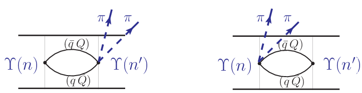
We now turn to the last two terms in (37), which contain two-pion vertex, shown in Fig.4, and take into account, that the dependence on there is contained in the factor , as was shown in [24, 25], as well as in the series shown in Fig.5 (and the similar one with ). Hence the total amplitude of transition with emission of two pions can be written as
| (43) |
where
| (44) |
One can see, that (43) satisfies Adler condition
| (45) |
and for not very large one can write approximately
| (46) |

The probability of transition is
| (47) |
and the dipion decay width is
| (48) |
where is the phase space factor
| (49) |
with the notations
| (50) |
Finally, one can also study the process , with the amplitude
| (51) |
where is given in (43) and so that the contribution of to the hadronic ratio is
| (52) |
We now turn to an example of possible pionic bottomonium state in the reaction , which can proceed through the chains
| (53) |
We are interested in possible poles in the channel of connected and states, which are given by the equation
| (54) |
Neglecting first nondiagonal elements of , one has an equation for
| (55) |
One can easily recognize in (55) the norm of the kernel of the integral equation (8).
| Threshold | Threshold | ||||
|---|---|---|---|---|---|
| 10.605 | 9.60 | ||||
| 10.650 | 10.16 | ||||
| 10.780 | 10.495 | ||||
| 10.830 | 10.720 | ||||
| 11.00 |
One can see, that the most important combination is with additional contribution of , and as a next step. Since the maximal energy of our systems in the reaction (53) is GeV, one is mostly interested in the energy region 9.78 GeV GeV.

V Results for
In this section we study numerical results for the reaction , and we shall be interested mainly in the possible appearance of resonance-like structures in the systems , . The resulting equations for differential and total probabilities are given in Eqs. (44), (46), (47), (48). The coefficients and parameters of and wave functions, needed for calculation of are given in Eqs.(29, 30) and Appendices 1 and 2.
It was assumed above, that the knowledge of wave functions and channel coupling constant (one for all types of strong decays) can describe all phenomena and, in particular, level shifts due to the . However, at this point one encounters the fundamental difficulty, which was studied in [36] and is not still resolved. The point is, that assuming a constant , not depending on participants of decay process, one obtains huge shifts of energy levels (several hundreds of MeV) due to mixing with higher states. (To improve situation, in [18] a cut-off coefficient was introduced for contribution of higher levels). This calls for a detailed scrutiny of our matrix elements and basic matrix elements (without hadron emission) , entering in the expressions for energy shifts, see [17] for details. Indeed in Eq. (2) one can see, that the string in the original hadron , placed between points is decaying at point into two hadrons, placed between , and respectively. It is clear, that when the point is far away from the center of the string , the string breaking process does not occur. Replacing distances between points by typical radii , of states one obtains condition (for ) , where is the typical string width, fm [37, 38]. The corresponding factor can be rigorously deduced in the formalism of [28], and the resulting cut-off strongly decreases the between states with incomparable sizes. This is taken into account below by assuming different for different decay channels. We take for the value GeV in case of . For we take and GeV respectively, to take into account decay mismatch between the sizes of and systems, since fm and fm, while fm. This mismatch is not taken into account for simplicity reasons in the general definition of the overlap integral (2).
In the beginning we have estimated and in (55) for , using parameters of SHO functions, which were used before in [25, 26], they are given in the Appendix 2. Real and imaginary parts of and are given in Fig.6. The possibility of peaks e.g. in system is demonstrated in Fig.7, where we plot the quantity for respectively (or more exactly the first term of (44)) as function of the invariant mass . One can see sharp peaks near the thresholds at 10.6 and 10.65 GeV respectively. In the total distributions, however, a more complicated combination of terms enters, as seen from (44), and one should calculate a symmetrized in expression, and moreover take into account appropriate phase space factor. One can associate these peaks with poles, situated in the vicinity of these thresholds (see discussion in Appendix 3).

Note, that two peaks in Fig.7 occur from combination . However in the full decay distribution the symmetrized sum (44) enters, which produces an additional mirror reflected pair of peaks in if considered as function of , since
| (56) |
The full probability distribution (47) contains symmetric sum of two rescattering series for and respectively. When plotted as function of it contains both poles of the first series at and GeV, and also poles from the second series at the points defined by Eq.(56). In this way one obtains Fig.8, where for the case and the secondary poles are out of mass interval, while for the case of the pair of secondary poles overlap with the proper poles of . In experiment one can separate points on Dalitz plot relating to and , which results in two plots with the same pair of peaks.
Recently experimental data on the reaction appeared in [34], and the experimental distributions are presented in Fig.5 of [34] as functions of and . In order to compare our results with experimental data, we calculate distribution (47) in terms of invariant masses of and systems. We use expressions (46), (49) and formulas from [24] to express quantities like etc. via variables . After integration over we obtain the distribution in terms of . The result is presented on Fig.8.

Comparing experimental data (left and right plots, glued together for and left plots for on Fig.5 from [34]) with our theoretical calculations, one can see a close similarity in the general form and position of and peaks, which in both cases appear at thresholds for all available . We do not intend to reproduce here all features of experimental data, which depend strongly on details of wave function profile, but we study mostly the dynamics of process. For the better description we only slightly changed w.f. of , presented in Appendix 2, by . A more detailed quantitative comparison of our data with experiment [34], and decay distributions as functions of and , are now in progress and will be reported elsewhere.
VI Conclusions and outlook
Summarizing our results, we shall stress the main features of our approach. We have considered the interaction of a light hadron with heavy quarkonium, arising solely due to transition to intermediate states of two heavy-light mesons. No direct interaction between light hadron and heavy quarkonium or else between two heavy-light mesons is assumed, therefore our dynamics has nothing to do with molecular states in the strict sense. Our mechanism is also distinct from dynamics of or hybrid states.
We have constructed explicitly transition vertex for the strong decay with emission of a light hadron from the first principles, and then all dynamics is defined by the overlap integrals of all wave functions involved, i.e. heavy quarkonia and heavy-light mesons. The latter have been found in [35] from the relativistic Hamiltonian, containing only first principle input, and accuracy of Gaussian representation was checked in [17, 32].
The answer given in Figs.7,8 is positive for the case of pion-bottomonium system, and agrees with the recent experimental data [34] at least qualitatively. More detailed calculations are still needed to check all results quantitatively experiment and this program is now under study. Other systems should be treated as well, e.g. , studied in [34], and the series of resonances in the system. All formalism used above for bottomonium can be applied to the charmonium case without modifications; for the vector charmonium or bottomonium ( one can use transition vertices, given in Appendices 1,2, and symmetry properties of the whole amplitude will be different. This work is now in progress.
One should stress at this point, that resonances, found above in system are specifically multichannel ones, in the sense, that they belong (and appear) in all channels and are given by zeros of .
At this point it is convenient to compare predictions of molecular and models for the positions of resonances. As one can see in Fig.7, our model predicts sharp peaks at thresholds (possibly due to virtual multichannel poles) in all channels, and this effect is due to combined contribution of and terms, i.e. pure effect. In contrast to that, the pure molecular picture, when poles in the systems appear due to direct internal interaction (i.e. without channels), the poles appear in all terms near corresponding thresholds. This can be seen simply in the definition of in (35), where is multiplied by the free Green’s function. In case of strong interaction in , systems, this Green function is replaced by the exact one and should contain pure molecular poles i.e. . Insertion of this form into the yields the -th order equation for roots in energy, and these roots are all strongly displaced from the original places at the thresholds for large coupling (large ), and are almost degenerate poles at thresholds for small coupling. Both pictures are different from the experimental data – the same two poles at and in all and channels. Thus the situation with the only pole at each threshold is possible and characteristic for our multichannel resonance and is unlikely for pure molecular states.
Another property is, that resonances appear most likely, when thresholds in and for some are close to each other, and then this channel will be the dominant one, making close to zero. In the case of the dominant channels are those with , as can be seen from Table in section 4. Therefore the visible channel ,where a peak is found, is not necessarily the dominant one, as might be in the case of with a peak seen in channel. The dynamical reason, why proximity of thresholds is favorable for the appearance of a resonance, is that both and are decreasing fast enough away from thresholds, making their product maximal for the coinciding thresholds.
In all discussion above the notion of resonances (or virtual and real poles) was stressed, and hence the whole sum of rescattering series as in Figs.3,5, were considered. But it is possible, that already the first terms of this series can contribute to enhanced correlations, which look like bumps in decay distributions. This approach was considered in two recent papers [39, 40], and is especially important in the case, when high spins and angular momenta are involved. Relation of this approach to our methods of present paper seems to be practically important and the corresponding work is planned for the future.
Recently several papers appeared [41, 42], where and are considered as molecular states and treated in the QCD sum rule method [41], while in [42] these states were originally supported to be and shifted to the and thresholds (as it happens in case). As was argued above in both cases the poles produced appear in and would be strongly shifted in the rescattering series of Fig.1, yielding 5 peaks at different masses in , .
In [43] an interesting analysis of decay is presented, demonstrating important contribution of to the decay distribution in and a detailed comparison of these results with our approach and previous results in [26] is now in progress.
The authors are grateful to A.M.Badalian, R.Mizuk and P.N.Pakhlov for many useful discussions. The financial support of Dynasty Foundation to V.D.O. and RFBR grant no.09-02-00 620a is gratefully acknowledged.
Appendix 1
Calculation of the transition kernel
We use here, as well as in [17, 24, 25] the spin-tensor representation of wave functions and factors instead of technic of Clebsch-Gordan coefficients. We start with the fully relativistic technic given in [24, 25], where can be written through the so-called factors (we omit the superscript for time being, cf. Eq.(A2.24) of [24])
| (A1.1) |
where and are factors for the total process and for individual hadrons respectively participating in the transition process or , shown in Fig.9. Defining projection factors for quarks and antiquarks , where subscript refers to light quarks, , or heavy quarks, , one can write
| (A1.2) |
| (A1.3) |
and
| (A1.4) |
Note, that the sum over (i) in (A1.4) is for also in the c.m. system , while is the current quark mass and is the average kinetic energy of quark in the hadron.
The operators correspond to quantum numbers of a hadron, and are given in Table 1 below, while refers to the process under investigation, for the case when no hadron is emitted, , while for the pion emission and for vector particles .
| form | ||||
|---|---|---|---|---|
| 1 | ||||
| - | ||||
| - | ||||
Here .


Examples of relativistic () expressions of are given in [24, 25], e.g. for and are given in (29),(30) while for
| (A1.6) |
We now turn to the case of formalism, introduced in [17], where resulting kernels are denoted as , and are computed according to
| (A1.7) |
while for emission of an additional pion in one should omit the factor in (A1.7). In this way one obtains (29), (30). Note, that normalization of states in ( formalism is different, and one should sum up over all polarizations in initial and final states (extra factor of is in (A1.7) as compared to (A1.6), and .
Of special interest are the transition kernels for states, where one has for and for , while the formalism yields
| (A1.8) |
For one has , and for are indices of polarizations.
Appendix 2
Wavefunctions of heavy quarkonia and heavy-light mesons
In Eq.(2) , and are series of oscillator wave functions, which are fitted to realistic wave functions. We obtain them from the solution of the Relativistic String Hamiltonian, described in [35].
In position space the basic SHO radial wave function is given by
| (A2.1) | |||
where is the SHO wave function parameter, and is an associated Laguerre polynomial. The realistic radial wave function can be represented as an expansion in the full set of oscillator radial functions:
| (A2.2) |
| State | ||||||
|---|---|---|---|---|---|---|
| Bottomonium | ||||||
| 1S | 1.27 | 0.977164 | -0.151779 | 0.141319 | -0.020857 | 0.036863 |
| 2S | 0.88 | -0.18823 | 0.953901 | -0.135824 | 0.181277 | -0.001509 |
| 3S | 0.76 | -0.128081 | -0.145885 | 0.936255 | -0.169962 | 0.226281 |
| 4S | 0.64 | -0.019432 | -0.149876 | -0.362548 | 0.88647 | 0.014308 |
| 5S | 0.6 | -0.011183 | -0.016911 | -0.182019 | -0.403138 | 0.853936 |
| 1P | 0.93 | 0.977994 | -0.165514 | 0.122975 | -0.018631 | 0.024364 |
| 2P | 0.76 | -0.092083 | 0.971982 | -0.137347 | 0.162174 | -0.002707 |
| 1D | 0.8 | 0.979042 | -0.168619 | 0.11132 | -0.016998 | 0.018383 |
| 2D | 0.69 | -0.063135 | 0.979871 | -0.117356 | 0.145358 | 0.000973 |
| Charmonium | ||||||
| 1S | 0.7 | 0.97796 | -0.169169 | 0.117682 | -0.019694 | 0.025113 |
| 2S | 0.53 | -0.121144 | 0.973054 | -0.130808 | 0.141495 | 0.00097 |
| 3S | 0.48 | -0.096897 | -0.086156 | 0.961504 | -0.155931 | 0.178935 |
| 4S | 0.43 | -0.021639 | -0.128342 | -0.215657 | 0.947215 | -0.028308 |
| 5S | 0.41 | -0.010701 | -0.022826 | -0.157891 | -0.258875 | 0.925921 |
| 1P | 0.57 | 0.976869 | -0.184163 | 0.105506 | -0.018941 | 0.017215 |
| 2P | 0.48 | -0.063059 | 0.981868 | -0.123012 | 0.127035 | 0.000588 |
| 1D | 0.51 | 0.979118 | -0.178313 | 0.095356 | -0.016095 | 0.013123 |
| 2D | 0.45 | -0.044316 | 0.986084 | -0.107408 | 0.117002 | 0.001907 |
| D meson | ||||||
| 1S | 0.48 | c=1 | ||||
| B meson | ||||||
| 1S | 0.49 | c=1 | ||||
Effective values of oscillator parameters and coefficients are obtained minimizing and listed in the Table 322 2 Typos of the sign convection are corrected for the charmonium states of [17]. In the momentum space the SHO radial wave function is given by 33 3 Note a typo in the equation for of [17]
| (A2.3) |
Then using Eq. (A16) from Appendix A of [25], one can write in (32) from as
| (A2.4) |
where
| (A2.5) |
| (A2.6) |
Here is the confluent hypergeometric series,
Appendix 3
Analytic structure of hadron-qurkonium resonances
At the end we study the analytic structure of the resonance denominator in , which in the one-channel case is given by Eq. (55). One can write as the integral
| (A3.1) |
where . To display the analytic properties of , we shall use the method, exploited in [17], Appendix E, i.e. we replace the integral in (A3.1) as 1/2 of the contour integral over the contour , circumjacent to the interval , as shown in Fig.10, and take in the physical region above the contour , . Deforming the contour, so that it passes above and to the left of the point (contour in Fig.10), using Cauchy’s theorem, one has the representation


| (A3.2) |
Here , and is analytic function in the neighborhood of the threshold . Hence acquires a negative contribution from the first term on the r.h.s. of (A3.2) and behaves, as shown in Fig.10. This behavior of and agrees with that, obtained by numerical integration in Fig.6.
In a similar way one can write the form of
| (A3.3) |
where , and are analytic and positive functions near the thresholds.
From (A3.2), (A3.3) one can deduce, that the product , is a real analytic function in the complex plane of with cuts, starting at thresholds and and going to plus infinity. Thus the combination is a real analytic function in the plane with positive weights in the integrals (A3.2), (A3.3). Hence the only possibility for the zeros of is on the real axis below thresholds, or else on the next sheets, which implies a standard situation with possibility of bound state or virtual state poles, or else Breit-Wigner poles in From (A3.2), (A3.3) one has
| (A3.4) |
In the simple case, when the thresholds in and coincide the resonance factor acquires the form
| (A3.5) |
with . This form demonstrates the appearance of a virtual or a real pole.
References
- [1] S. -K. Choi et al. (Belle Collaboration), Phys. Rev. Lett. 94, 182002 (2005); B. Aubert et al. (BABAR Collaboration), Phys. Rev. Lett. 101, 082001 (2008); Phys. Rev. D 79, 112002 (2009).
- [2] S. -K. Choi, S. L. Olsen et al. (Belle Collaboration), Phys. Rev. Lett. 100, 142001 (2008).
- [3] R. Mizuk, et al. (Belle Collaboration), Phys. Rev. D 78, 072004 (2008); ibid D 80, 031104 (2009).
- [4] T. Aaltonen et al. (CDF Collaboration), Phys. Rev. Lett. 102, 242002 (2009); arXiv: 1101.6058 [hep-ex].
- [5]
G.V. Pakhlova, Plenary talk at ICHEP 08, Philadelphia,
USA arXiv:0810.4114; G.V. Pakhlova, P.N. Pakhlov, and
S.I. Eidelman, Phys. Usp. 53, 219 (2010);
A.G.Mokhtar and S.L.Olsen, arXiv:1101.22 [hep-ex]. - [6] X. Liu, Y. R. Liu, W. -Z. Deng, S. L. Zhu, Phys. Rev. D 77, 034003 (2008).
- [7] S. H. Lee, K. Morita, M. Nielsen, Nuc. Phys. A 815, 29 (2009).
- [8] X.-H. Liu, Q. Zhao, F. E. Close, Phys. Rev. D 77, 094005 (2008).
- [9] D. Dubynskiy, M. B. Voloshin, Phys. Lett. B 666, 344 (2008).
- [10] D. V. Bugg, J. Phys. G 35 , 075005 (2008).
- [11] Youchang Yang, Zurong Xia, Jialun Ping, arXiv: 0912.5061v1 [hep-ph].
- [12] X. Liu, Z. G. Luo, Y. R. Liu, and S. L. Zhu, Eur. Phys. J. C 61, 411 (2009).
- [13] X. Liu, and S. L. Zhu, Phys. Rev. D 80, 017502 (2009).
- [14] T. Branz, T. Gutsche, V. E. Lyubovitskij, Phys. Rev. D 80, 054019 (2009).
- [15]
Jian-Rong Zhang and Ming-Qiu Huang, Phys. Rev. D 80, 056004
(2009);
N.A.Tornqvist, Phys. Rev. Lett. 67, 556 (1991); Z.Phys. C61, 525 (1994);
X. Liu,Z.-G. Luo and S. L. Zhu, arXiv:1011.1045[hep-ph]. - [16] Yan-Rui Liu, Zong-Ye Zhang, Phys. Rev. C 80, 015208 (2009).
- [17] I. V. Danilkin, Yu. A. Simonov, Phys. Rev. D 81, 074027 (2010).
- [18] I. V. Danilkin, Yu. A. Simonov, Phys. Rev. Lett. 105, 102002.
- [19] H. Y. Cheng, C. K. Chua and A. Soni, Phys. Rev. D71, 014030 (2005).
- [20] X. Liu, B. Zhang and S. L. Zhu, Phys. Lett. B 645, 185 (2007).
- [21] C. Meng and K. T. Chao, Phys. Rev. D 75, 114002 (2007).
- [22] C. Meng and K. T. Chao, arXiv: 0708.4222 [hep-ph].
- [23] C. Meng and K. T. Chao, Phys. Rev. D 77, 074003 (2008).
- [24] Yu. A. Simonov, Phys. At. Nucl. 71, 1048 (2008).
- [25] Yu. A. Simonov, A. I. Veselov, Phys. Rev. D 79, 034024 (2009).
- [26] Yu. A. Simonov, A. I. Veselov, Phys. Lett. B 671, 55 (2009), ibid B 673, 211 (2009).
- [27] Yu.A.Simonov, A.I.Veselov, JETP Lett. 88, 5 (2008).
- [28] Yu.A.Simonov, Phys. Rev. D 84, 065013 (2011).
- [29] A. M. Badalian, L P. Kok, M. I. Polikarpov and Yu. A.Simonov, Phys. Rept. 82, 31 (1982).
- [30] K. Abe et al. (Belle Collaboration), arXiv; hep-ex/0505037 (2005).
- [31] D. Liventsev (for Belle Collaboration), arXiv: 1105. 4760 [hep-ex].
- [32] E. van Beveren and G. Rupp, Ann. Phys. 324, 1620 (2009); Int. J. Theor. Phys. Group Theor. Nonlin. Opt. 11, 179 (2006).
- [33] S. Coito, G. Rupp and E. van Beveren, arXiv: 1008.5100.
- [34] I. Adachi et al. (Belle Collaboration), arXIv: 1105. 4583 [hep-ex].
- [35] A. M. Badalian and B. L. G. Bakker, J. Phys. G 31, 417 (2005); A. M. Badalian and I. V. Danilkin, Phys. Atom. Nucl. 72, 1206 (2009); A. M. Badalian, B. L. G. Bakker, and I. V. Danilkin, Phys. Atom. Nucl. 72, 638 (2009); Phys. Rev. D 79, 037505 (2009); A. M. Badalian and B. L. G. Bakker, Phys. Lett. B 646, 29 (2007), Phys. Atom. Nucl. 70, 1764 (2007); A.M. Badalian and I.V. Danilkin, Phys. Atom. Nucl. 72, 1206 (2009), arXiv:0801.1614.
- [36] P. Geiger, N. Isgur, Phys. Rev. D 41, 1595 (1990).
- [37] N. Cardoso, M. Cardoso, P. Bicudo, [arXiv:1108.1542 [hep-lat]].
- [38] P.S.Kuzmenko, V.I.Shevchenko, Yu.A.Simonov, Phys.Usp. 174 (2004) 3-18 DOI: 10.3367/UFNr.0174.200401a.0003
- [39] A.E.Bondar, A.Garmash, A.I.Milstein, R.Mizuk and M.B.Voloshin, arXiv: 1105.4473 [hep-ph].
- [40] P.Pakhlov, arXiv: 1105.2945 [hep-ph].
- [41] Jian-Rong Zhang, Ming Zhong and Ming-Qiu Huang, arXiv: 1105.5472 [hep-ph].
- [42] D.V.Bugg, arXiv: 1105.5492 [hep-ph].
- [43] Dian-Yong Chen, Xiang Liu and Shi-Lin Zhu, arXiv: 1105.5193 [hep-ph].