Doublon production rate in modulated optical lattices

Akiyuki Tokuno Affiliation: DPMC-MaNEP, University of Geneva, 24 Quai Ernest-Ansermet CH-1211 Geneva, Switzerland. Eugene Demler Affiliation: Department of Physics, Harvard University, Cambridge, MA 02138. Thierry Giamarchi Affiliation: DPMC-MaNEP, University of Geneva, 24 Quai Ernest-Ansermet CH-1211 Geneva, Switzerland.

August 24, 2026

Abstract

We study theoretically lattice modulation experiments with ultracold fermions in optical lattices. We focus on the regime relevant to current experiments when interaction strength is larger than the bandwidth and temperature is higher than magnetic superexchange energy. We obtain analytical expressions for the rate of doublon production as a function of modulation frequency, filling factor, and temperature. We use local density approximation to average over inhomogeneous density for atoms in a parabolic trap and find excellent agreement with experimentally measured values. Our results suggest that lattice modulation experiments can be used for thermometry of strongly interacting fermionic ensembles in optical lattices.

pacs

05.30.Fk,71.10.Fd,78.47.-p

I Introduction

Cold atoms provide a new platform in which one can explore long standing open questions of strongly correlated systems in condensed matter physics [1, 2]. In particular, two-component Fermi mixtures in an optical lattice provide an ideal realization of the fermionic Hubbard model, where two species of fermions – corresponding to the spin $1/2$ – interact with an on-site repulsion. This model is relevant for understanding properties of electrons in several classes of novel quantum materials including oxides and high- $T_{c}$ superconductors [3, 4]. There are currently many efforts to probe the low-temperature physics of such a model, with experiments already demonstrating the Mott insulating behavior expected in this model [5, 6].

An important feature of strongly correlated ultracold atoms is that traditional probes used in solid state physics are often not readily available. One thus needs to understand how experimental techniques appropriate for atomic ensembles can provide information on many-body states. In this paper we focus on understanding lattice modulation experiments with fermions in optical lattices. The technique of lattice modulation was originally introduced for bosonic systems and absorbed energy was measured as a function of modulation frequency [7]. Measuring energy absorption, however, can not be done accurately enough for strongly interacting fermions. Thus an extension of this technique was proposed, [8] and implemented [9], in which the number of doubly occupied sites created by the lattice modulation was measured. Recent experiments successfully reached the regime of weak perturbations in which the number of doublons created scales quadratically with the modulation amplitude (Fermi’s golden rule) and the modulation pulse duration [9].

While theoretical understanding of such experiments with bosons is now relatively complete [10, 11, 12], the case of fermions turned out to be more challenging. The main difficulty is the presence of excitations at very different energy scales: high-energy charge excitations, so-called doublons and holons, that have energies set by the on-site repulsion $U$ and fermion hopping strength $J$ , and magnetic excitations that have energies of the order of superexchange energy $J^{2}/U$ . Understanding the interplay of charge and spin degrees of freedom in the Hubbard model is a long standing problem in condensed matter physics [13, 14]. In the special case of half filling and fully disordered spin states, analysis of lattice modulation experiments has been performed previously [15, 16]. However, such analysis is not sufficient for quantitative comparison to experiments which are done with systems in a parabolic potential that have a large number of atoms outside of the incompressible Mott plateaus.

Furthermore such real-time dynamics at finite temperature as seen in current experiments is problematic for numerics. Monte Carlo simulations [17] suffer from the problems of analytic continuation. Density-matrix renormalization group approaches, which can deal with real time dynamics, are so far limited to one dimension. Therefore, a comparison of dynamical quantities to experiments is a non-trivial theoretical subject.

In this paper we develop another analytical approach to calculate finite-temperature dynamics, that is, the doublon production rate (DPR), based on the slave-particle technique [18, 15, 19]. This approach is particularly adapted to the paramagnetic phase of the Hubbard model, and can be applied to any filling of the band and finite temperatures whose region is relevant to ongoing experiments. It provides a remarkable agreement to the experiments and allows for potential extensions.

This paper is organized as follows. We define the system Hamiltonian, and introduce the slave-particle representation in Sec. II. In Sec. III, the spectral functions of the slave particles are evaluated, and in addition the spectral function of the original fermionic atom is also obtained. In Sec. IV, we proceed with the estimation of the doublon production rate based on the obtained spectral functions in Sec. III, and the analytic formula of the DPR spectrum is given. In Sec. V, the obtained analytic formula is extended to an inhomogeneous system in a trap by the local density approximation (LDA), and a comparison with the experiment in Ref. [9] is implemented. Finally, Sec. VI is devoted to the summary.

II Slave particle representation

We consider the Hubbard model $H_{0}=H_{\rm K}+H_{\rm at}$ with


		$\displaystyle H_{\rm K}=-J\sum_{\sigma,\langle{i,j}\rangle}c^{\dagger}_{i\sigma}c_{j\sigma},$		(1a)
		$\displaystyle H_{\rm at}=-\mu\sum_{j,\sigma}n_{j\sigma}+U\sum_{j}n_{j\uparrow}n_{j\downarrow},$		(1b)

where $c^{\dagger}_{j\sigma}$ and $n_{j\sigma}=c^{\dagger}_{j\sigma}c_{j\sigma}$ are, respectively, a creation and number operator of a spin- $\sigma$ fermions at a $j$ th site. We use the following slave-particle representation:

c^{\dagger}_{j\uparrow}=b^{\dagger}_{j\uparrow}h_{j}+b_{j\downarrow}d^{\dagger}_{j},\qquad c^{\dagger}_{j\downarrow}=b^{\dagger}_{j\downarrow}h_{j}-b_{j\uparrow}d^{\dagger}_{j},

(2)

where $b^{\dagger}_{j\sigma}$ , $h^{\dagger}_{j}$ and $d^{\dagger}_{j}$ are, respectively, creation operators of a slave boson of spin- $\sigma$ state (Schwinger boson), holon and doublon at a site $j$ . They satisfy the (anti-)commutation relations, $[b_{i\sigma},b^{\dagger}_{j\sigma^{\prime}}]=\delta_{i,j}\delta_{\sigma,\sigma^{\prime}}$ and $\{h_{i},h_{j}^{\dagger}\}=\{d_{i},d_{j}^{\dagger}\}=\delta_{i,j}$ . The enlarged Hilbert space is projected onto the physical one by the following constraint at every site:

\sum_{\sigma}b^{\dagger}_{j\sigma}b_{j\sigma}+h^{\dagger}_{j}h_{j}+d^{\dagger}_{j}d_{j}=1.

(3)

Equation (2) allows us to rewrite the Hamiltonian (1) as

		$\displaystyle H_{\rm K}=J\sum_{\langle i,j\rangle}\left[F_{ji}(h_{i}^{\dagger}h_{j}-d_{i}^{\dagger}d_{j})+(A_{ij}^{\dagger}d_{j}h_{i}+{\rm H.c.})\right],$		(4)
		$\displaystyle H_{\rm at}=\sum_{j}\left[\epsilon^{\rm d}_{j}d^{\dagger}_{j}d_{j}+\epsilon^{\rm h}_{j}h^{\dagger}_{j}h_{j}+\sum_{\sigma}\epsilon^{\rm b}_{j}b^{\dagger}_{j\sigma}b_{j\sigma}-\lambda_{j}\right],$		(5)

where $F_{ji}=\sum_{\sigma}b^{\dagger}_{j\sigma}b_{i\sigma}$ and $A^{\dagger}_{ij}=b^{\dagger}_{i\uparrow}b^{\dagger}_{j\downarrow}-b^{\dagger}_{j\downarrow}b^{\dagger}_{i\uparrow}$ mean the hopping of slave bosons and the creation of spin singlet pair, respectively. The local potentials of a slave boson, holon, and doublon are, respectively, defined as $\epsilon^{\rm b}_{j}=\lambda_{j}$ , $\epsilon^{\rm h}_{j}=\mu+\lambda_{j}$ , and $\epsilon^{\rm d}_{j}=U-\mu+\lambda_{j}$ . The constraint (3) is implemented via the Lagrange multiplier $\lambda_{j}$ .

III Diagrammatic analysis

III.1 Atomic limit

We start with the atomic limit ( $J/U=0$ ). Then the kinetic term (4) which describes the scattering among slave particles vanishes. Since the atomic Hamiltonian (5) is quadratic, the atomic propagators at $j$ th site are easily obtained as

{\cal G}^{(0)}_{{\rm b}\sigma}(\bm{r}_{j},i\omega_{n})=\frac{1}{i\omega_{n}-\epsilon^{\rm b}_{j}},\quad{\cal G}^{(0)}_{\rm d/h}(\bm{r}_{j},i\nu_{n})=\frac{1}{i\nu_{n}-\epsilon^{\rm d/h}_{j}},

(6)

where $\omega_{n}$ and $\nu_{n}$ are the Matsubara frequency for bosons and fermions, respectively. Note that the atomic limit propagators of slave bosons are independent of the spin. This means that the atomic limit exhibits spin-incoherent paramagnetism. Hereafter we set $\hbar=1$ .

Let us suppose the mean-field (MF) $\lambda_{j}$ to be determined by the atomic limit. Namely, the self-consistent equation for $\lambda_{j}$ corresponds to the statistical average of the constraint (3) in the atomic limit:

2b(\epsilon_{{\rm b},j})+f(\epsilon_{{\rm h},j})+f(\epsilon_{{\rm d},j})=1,

(7)

where the prefactor $2$ comes from the spin degrees of freedom. $f(\epsilon)$ and $b(\epsilon)$ are, respectively, the Fermi and Bose distribution functions. One can expect that if the effect of the kinetic energy $H_{\rm K}$ is small, that is, at relatively high temperature compared to the kinetic energy, the validity of this treatment should be guaranteed. We thus use the MF assumption for the Lagrange multiplier: $\lambda_{j}\rightarrow\lambda$ . Simultaneously the local potentials are also replaced by the homogeneous ones: $\epsilon^{\rm x}_{j}\rightarrow\epsilon_{\rm x}$ where ${\rm x}={\rm b},{\rm h},{\rm d}$ . Corresponding to the MF treatment for the Lagrange multiplier, the atomic propagators also become independent of sites: For example, the replacement of $\lambda_{j}\rightarrow\lambda$ leads the slave boson propagator $\mathcal{G}_{\mathrm{b}\sigma}^{(0)}(\bm{r}_{j},i\omega_{n})\rightarrow\bar{\mathcal{G}}_{\mathrm{b}}(i\omega_{n})$ where the site-independent propagator is defined as

\bar{\mathcal{G}}_{\mathrm{b}}(i\omega_{n})=\frac{1}{i\omega_{n}-\epsilon_{\mathrm{b}}}.

(8)

Let us solve the self-consistent equation (7). For $k_{B}T/U\ll 1$ , Eq. (7) can be simplified, and solved analytically as follows:

\lambda=k_{B}T\log\frac{3+\sqrt{9+8(e^{-(U-\mu)/k_{B}T}+e^{-\mu/k_{B}T})}}{2}.

(9)

As discussed below, Eq. (7) is numerically solved, and we compare the numerical result with Eq. (9). The obtained $\lambda$ leads the estimation of the slave particle densities. The density of each slave particle is given by the MF solution $\lambda$ : $n_{\sigma}^{\mathrm{MF}}=b(\epsilon_{\mathrm{b}})$ for a slave boson, $n_{\mathrm{h}}^{\mathrm{MF}}=f(\epsilon_{\mathrm{h}})$ for a holon and $n_{\mathrm{d}}^{\mathrm{MF}}=f(\epsilon_{\mathrm{d}})$ for a doublon. The temperature and chemical potential dependency of them are shown in Fig. 1. In the temperature region shown in Fig. 1, the results analytically given by Eq. (9) are in precise agreement with ones given by the numerically solved $\lambda$ .

Refer to caption — Figure 1: (cClor online) The slave-particle densities as a function of temperature for different chemical potentials: (a) the slave boson, (b) holon, and (c) doublon density. The chemical potentials are chosen as follows: $\mu/U=0.5$ , $0.2$ , $0.1$ , and $0$ from the top to bottom. The MF results $n_{\sigma}^{\mathrm{MF}}$ , $n_{\mathrm{h}}^{\mathrm{MF}}$ , and $n_{\mathrm{d}}^{\mathrm{MF}}$ given by the slave-particle technique and the exact results in the atomic limit, $n_{\sigma}$ , $n_{\mathrm{h}}$ , and $n_{\mathrm{d}}$ , are compared. $n_{\sigma}^{\mathrm{MF}}$ , $n_{\mathrm{h}}^{\mathrm{MF}}$ , and $n_{\mathrm{d}}^{\mathrm{MF}}$ are calculated numerically and analytically. The solid, dashed, and dotted lines, respectively, denote the exact result by the atomic limit calculation, the slave particle approach (22).

It means that in such a regime we may always employ Eq. (9) as a solution of the MF self-consistent equation (7). On the other hand, the densities in the atomic limit can be exactly calculated as shown in Appendix A. Here we take the exact densities to be $n_{\sigma}$ , $n_{\mathrm{h}}$ and $n_{\mathrm{d}}$ , and their temperature and chemical potential dependency is also shown in Fig. 1. The exact result allows us to discuss the temperature and chemical potential regime justifying the slave particle approach. From the comparison made in Fig. 1, the slave particle technique is found to agree with the exact result in the temperature and chemical potential region where $n_{\sigma}^{\mathrm{MF}}=1/2$ and $n_{\mathrm{h}}^{\mathrm{MF}}=n_{\mathrm{d}}^{\mathrm{MF}}=0$ . In other words the slave particle technique is expected to be reasonable when the system is near a Mott insulator, and such temperature as a benchmark is below $k_{B}T/U\approx 0.1$ .

III.2 The finite hopping

We now consider a finite but small hopping by taking the infinite series of diagrams produced by the scattering $H_{\rm K}$ among the slave particles, based on the non-crossing (NC) approximation [13, 14]. This approximation can be also regarded as a certain type of high temperature series expansion (HTSE) [20], but in our formalism the Wick theorem is still applicable due to the quadratic Hamiltonian (5), and a particular infinite series of kinetic energy perturbation can be taken. Based on the NC approximation the self-energy diagrams constructed by full propagators, shown in Fig. 2, are considered.

Since one is in a temperature regime higher than the anti-ferromagnetic exchange $\sim 4J^{2}/U$ , we apply the spin-incoherent assumption to the slave boson propagator. Namely, the slave boson propagators in the diagrams of Fig. 2 are replaced by the atomic one (8),

\tilde{\mathcal{G}}_{\rm{b}\sigma}(\bm{k},i\omega_{n})\rightarrow\bar{\mathcal{G}}_{\mathrm{b}}(i\omega_{n}).

(10)

The doublon and holon propagators are left full ones: namely, by using the Dyson equation the full propagators are written as

	$\displaystyle\tilde{\mathcal{G}}_{\mathrm{d/h}}(\bm{k},i\nu_{n})$	$\displaystyle=\tilde{\mathcal{G}}^{(0)}_{\mathrm{d/h}}(\bm{k},i\nu_{n})$
		$\displaystyle\quad+\tilde{\mathcal{G}}^{(0)}_{\mathrm{d/h}}(\bm{k},i\nu_{n})\tilde{\Sigma}_{\mathrm{d/h}}(\bm{k},i\nu_{n})\tilde{\mathcal{G}}_{\mathrm{d/h}}(\bm{k},i\nu_{n}).$		(11)

Unlike the standard MF theory, the dynamical fluctuation of the slave bosons is retained here, which is necessary to describe the doublon-holon excitation. The NC diagram Fig. 2 (b) couples the self-consistent equations of the doublon and holon self-energy. However, the contribution is negligibly small because it is a far off-shell diagram in this case such as Mott state. Consequently the self-consistent equations of the self-energy Fig. 2 (a) are decoupled and one can obtain in momentum space,

\tilde{\Sigma}_{\rm d}(\bm{k},i\nu_{n})=\frac{W^{2}}{4}\frac{1}{N}\sum_{\bm{p}}\tilde{\mathcal{G}}_{\rm d}(\bm{p},i\nu_{n}).

(12)

with $W=\sqrt{8zb(\epsilon_{\rm b})[b(\epsilon_{\rm b})+1]J^{2}}$ corresponding to a half band width for the holon and doublon as we will see below. $z$ is a coordination number, and $N$ is the total site number of the system. Note that due to the momentum dependence of the right-hand side the self-energy should be given as a local quantity: $\tilde{\Sigma}_{\rm d}(\bm{k},i\nu_{n})=\Sigma_{\rm d}(i\nu_{n})$ . Consequently the propagator also turns out to be local: $\tilde{\mathcal{G}}_{\mathrm{d}}(\bm{k},i\nu_{n})=\mathcal{G}_{\mathrm{d}}(i\nu_{n})$ . Thus the self-consistent equation (12) is easily solved through the Dyson equation (11) as follows:

\Sigma_{\rm d}(i\nu_{n})=\frac{i\nu_{n}-\epsilon_{\rm d}-i\sqrt{W^{2}-(i\nu_{n}-\epsilon_{\rm d})^{2}}}{2}.

(13)

Through the analytic continuation the doublon spectral function, which is equivalent to the density of state (DOS) in this case, is also obtained. In this approximation, a semi-circle type DOS is formed:

{\cal A}_{\rm d}(\omega)=\frac{4}{W}\sqrt{1-\left(\frac{\omega-\epsilon_{\rm d}}{W}\right)^{2}}.

(14)

One can also obtain the self-energy and spectral function of the holon in the same way. The forms are the same as what is obtained by the replacement $\epsilon_{\mathrm{d}}\rightarrow\epsilon_{\mathrm{h}}$ in Eqs. (13) and (14). The holon spectral function is found to reasonably reproduce the result of Brinkman and Rice on single hole dynamics in a Mott insulator [13]. The chemical potential dependency of the band width $W$ is shown in Fig. 3.

Using the representation (2), via the Matsubara Green’s function of the original fermion, the DOS (spectral function) is represented as

	$\displaystyle{\cal A}_{\sigma}(\omega)$	$\displaystyle=\biggl[b(\epsilon_{\rm b})+f(\epsilon_{\rm b}-\omega)\biggr]{\cal A}_{\rm h}(\epsilon_{\rm b}-\omega)$
		$\displaystyle\quad+\biggl[b(\epsilon_{\rm b})+f(\epsilon_{\rm b}+\omega)\biggr]{\cal A}_{\rm d}(\epsilon_{\rm b}+\omega).$		(15)

As expected, the doublon and holon spectral functions, ${\cal A}_{\rm d}$ and ${\cal A}_{\rm h}$ , give the upper and lower Hubbard band, respectively. The spectral function as a function of $J/U$ and the chemical potential is shown in Fig.4.

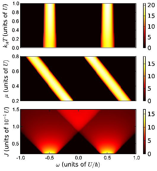
IV Doublon production rate

We calculate the DPR induced by the amplitude modulation of an optical lattice potential using the above formalism. The amplitude modulation of the optical lattice potential, $V(t)=V_{0}+\delta{V}\cos(\omega t)$ , modifies both $J$ and $U$ as $J\rightarrow J[1+\delta{J}\cos(\omega t)]$ and $U\rightarrow U[1+\delta{U}\cos(\omega t)]$ , where $\delta{J}$ and $\delta{U}$ are dimensionless modulation perturbation parameters and given as a function of $\delta{V}$ . However, it is possible to map the two parameter modulations problem to single parameter one of either $J$ or $U$ [10, 11, 8, 15]. Namely, the modulation perturbation to be discussed here can be written as

H_{\rm mod}(t)=\delta{F}\cos(\omega t)H_{\rm K},

(16)

where $\delta{F}=\delta{J}-\delta{U}$ . ¹¹ 1 There is a slight additional modification coming from the presence of the trap in this formula, but this does not change quantitatively the results for the case considered here Within the second-order perturbation in terms of $\delta{F}$ , the DPR defined as the time averaged growth rate of atoms forming doublons is given as [8]

P_{\rm D}(\omega)=-\frac{(\delta{F})^{2}}{U}\omega\Im{{\chi}^{\rm R}_{\rm K}(\omega)},

(17)

where ${\chi}^{\rm R}_{\rm K}(\omega)=-i\int_{0}^{\infty}\!\!dt\ e^{i\omega t}\langle[H_{\rm K}(t),H_{\rm K}(0)]\rangle$ . As shown in Appendix B, we represent the correlation function $\chi_{\mathrm{K}}(\tau)=-\langle{T_{\tau}H_{\mathrm{K}}(\tau)H_{\mathrm{K}}(0)}\rangle$ without vertex corrections in the slave-particle description ²² 2 The vertex corrections give at least the correction of ${\cal O}((J/U)^{4})$ . In addition, it does not affect crucially in the insulator with the large Mott gap.,

	$\displaystyle\chi_{\rm K}(\tau)$	$\displaystyle=-2J^{2}\sum_{\langle{i,j}\rangle}\{\Gamma_{ij}^{\mathrm{h}}(\tau)\bar{\mathcal{G}}_{\mathrm{b}}(\tau)\bar{\mathcal{G}}_{\mathrm{b}}(-\tau)+\Gamma_{ij}^{\mathrm{d}}(\tau)\bar{\mathcal{G}}_{\mathrm{b}}(\tau)\bar{\mathcal{G}}_{\mathrm{b}}(-\tau)$
		$\displaystyle\quad-[\bar{\mathcal{G}}_{\mathrm{b}}(-\tau)]^{2}\mathcal{G}_{\mathrm{h}}(\tau)\mathcal{G}_{\mathrm{d}}(\tau)-[\bar{\mathcal{G}}_{\mathrm{b}}(\tau)]^{2}\mathcal{G}_{\mathrm{h}}(-\tau)\mathcal{G}_{\mathrm{d}}(-\tau)\},$		(18)

where $\Gamma_{ij}^{\mathrm{X}}(\tau)=\langle{T_{\tau}x_{i}^{\dagger}(\tau)x_{j}(\tau)x_{j}^{\dagger}(0)x_{i}(0)}\rangle$ ( $x=d$ or $h$ ) is a two-particle Green’s function of a doublon ( $\mathrm{X}=\mathrm{d}$ ) and holon ( $\mathrm{X}=\mathrm{h}$ ). The diagrams corresponding to the terms in Eq. (18) are illustrated in Fig. 5. Without the vertex correction, the two-particle propagators are contracted to a single particle propagators by the Wick expansion: $\Gamma_{ij}^{\rm X}(\tau)=-{\cal G}_{\rm X}(\tau){\cal G}_{\rm X}(-\tau)$ . Through the Fourier transform of $\chi_{\rm K}(\tau)$ and analytic continuation, one can straightforwardly obtain the real-time kinetic energy correlation function in frequency domain. As a result, the imaginary part of the correlation function is given as

$\displaystyle\frac{\Im{\chi_{\rm K}^{\rm R}(\omega)}}{-NW^{2}/8}$	$\displaystyle=\int\!\!\frac{d\nu}{2\pi}[f(\nu-\omega)-f(\nu)][{\cal A}_{\rm h}(\nu){\cal A}_{\rm h}(\nu-\omega)$
	$\displaystyle\quad+{\cal A}_{\rm d}(\nu){\cal A}_{\rm d}(\nu-\omega)]+2\sinh(\epsilon_{\rm b})\int\!\!\frac{d\nu}{2\pi}[b(2\epsilon_{\rm b})$
	$\displaystyle\quad+f(\nu)]\{[f(2\epsilon_{\rm b}-\nu)-f(2\epsilon_{\rm b}-\nu+\omega)]$
	$\displaystyle\quad\times{\cal A}_{\rm d}(\nu){\cal A}_{\rm h}(2\epsilon_{\rm b}+\omega-\nu)-(\omega\rightarrow-\omega)\}.$	(19)

V Comparison with experiments

Let us compare our result (19) with the experimental data. We employ a set of the parameters evaluated in the ⁴⁰K atom experiment [9]: the hopping $J/\hbar=2\pi\times 85$ (Hz) and the interaction $U/\hbar=2\pi\times 5400$ (Hz). In terms of the optical lattice potential, the depth, modulation rate and lattice constant are, respectively, taken to be $V_{0}=10E_{\rm R}$ where $E_{\rm R}$ is a recoil energy, $\delta{V}/V_{0}=0.1$ and $a=532$ (nm). The lattice modulation is translated into $\delta{F}\approx-0.32$ in hopping modulation. The LDA is used to take into account the effect of the harmonic trap potential $V_{\rm trap}(\bm{r})$ whose frequency is $(\omega_{x}/2\pi,\omega_{y}/2\pi,\omega_{z}/2\pi)=(56,61,139)$ (Hz). In the LDA, we replace the chemical potential of the homogeneous case by the local one, $\mu(\bm{r})=\mu_{0}-V_{\rm trap}(\bm{r})$ where $\mu_{0}$ is self-consistently determined to give the total trapped atom number $8\times 10^{4}$ . In our framework, temperature is treated as a free parameter so that we determine the temperature by a fit of the DPR spectrum intensity at $\omega=U/\hbar$ , which is obtained in the experiment.

The temperature dependence of the DPR spectrum at $\omega=U/\hbar$ is shown in the inset in Fig. 6, and $k_{\rm B}T/U\approx 0.052$ in this system is determined.³³ 3 A least square fit has been also implemented, and gives the similar result $k_{B}T/U\approx 0.045$ . The determined temperature is in the region to justify the slave-particle approach, which is discussed in Sec. III, and the theory is thus expected to work well. Furthermore, using the obtained temperature, we plot the DPR spectrum in Fig. 6. The agreement is remarkably good. In addition to giving access to the line shape it means that via our theory one can use the shaking method as a good thermometer in low temperature regime ⁴⁴ 4 In contrast the HTSE would be instead better in the higher temperature region, as discussed in Ref. [25], since the curve giving the amplitude versus temperature (the inset in Fig. 6) is reasonably smooth and steep. To check this point we compare in our case the temperature determined by the fitting of the shaking curve with other estimates from entropy calculations [25] and find that the two results are perfectly consistent.

VI Conclusion and summary

In this paper, we have described the charge excitation of strongly correlated fermionic systems in the spin-incoherent paramagnetic regime by a slave-particle representation and diagrammatic approach from the atomic limit. This method allows us to take the finite temperature and trapping into account. Based on the spectrum functions of the doublon and holon, the analytical form of the DPR spectrum as a second-order response of the optical lattice modulation has been given, and extended to the homogeneous system of the trapped atom cloud by using the local density approximation. In addition, substituting the parameters evaluated in the experiment [9], a comparison with the experiment has been made. Although temperature has not been directly measured in experiments, it has been determined as an optimization parameter which is controlled to fit the experimental data. The result has been in agreement with the experimental data, which shows that one can use the lattice modulation spectroscopy as a thermometer.

Our method has potential extension such as SU( $N$ ) higher symmetric atom systems realized in alkaline-earth-metal atom experiments. [26, 27, 28, 29]

Acknowledgements.

We are grateful to C. Berthod, T. Esslinger, D. Greif, N. Kawakami, A. Koga, L. Pollet, L. Tarruell, and T. Uehlinger for fruitful discussions. In addition, we thank D. Pekker for contributions at an early stage of this work and T. Esslinger’s group for making their data available. ED acknowledges support from the DARPA OLE program, Harvard-MIT CUA, NSF Grant No. DMR-07-05472, AFOSR Quantum Simulation MURI. This work was supported by the Swiss National Foundation under MaNEP and division II.

Appendix A The slave-particle density in the atomic limit

In order to clarify the parameter regime to justify the slave-particle approach, we make a comparison with the exact calculation in the atomic limit. Then we focus on the single site occupations as a function of temperature and chemical potential, which is identical to the densities of the slave boson, holon, and doublon.

Let us perform the atomic limit calculation. We consider the atomic Hamiltonian (1b). Then the partition function is calculated as

Z_{\mathrm{atom}}=1+2x+x^{2}y

(20)

where $x=e^{\mu/K_{B}T}$ and $y=e^{-U/k_{B}T}$ . To calculate the densities of the slave boson, holon, and doublon, we introduce the projection operators. In the original fermion picture, the projection operators of the slave boson, holon and doublon state are, respectively, written as $p_{\sigma}=n_{\sigma}-n_{\uparrow}n_{\downarrow}$ , $p_{\mathrm{h}}=(n_{\uparrow}-1)(n_{\downarrow}-1)$ , and $p_{\mathrm{d}}=n_{\uparrow}n_{\downarrow}$ . They obviously obeys the constraint $\sum_{\sigma}p_{\sigma}+p_{\mathrm{h}}+p_{\mathrm{d}}=1$ . Taking the statistical average of these projection operators, we obtain the following exact result of slave-particle densities:


$\displaystyle n_{\sigma}$	$\displaystyle=\langle{p_{\sigma}}\rangle=\frac{x}{1+2x+x^{2}y},$	(21a)
$\displaystyle n_{\mathrm{h}}$	$\displaystyle=\langle{p_{\mathrm{h}}}\rangle=\frac{1}{1+2x+x^{2}y},$	(21b)
$\displaystyle n_{\mathrm{d}}$	$\displaystyle=\langle{p_{\mathrm{d}}}\rangle=\frac{x^{2}y}{1+2x+x^{2}y}.$	(21c)

On the other hand, in the case of the slave-particle approach combined with the MF solution of the Lagrange multiplier $\lambda$ , the slave-particle densities are given as


	$\displaystyle n_{\sigma}^{\mathrm{MF}}=b(\epsilon_{\mathrm{b}}),$		(22a)
	$\displaystyle n_{\mathrm{h}}^{\mathrm{MF}}=f(\epsilon_{\mathrm{h}}),$		(22b)
	$\displaystyle n_{\mathrm{d}}^{\mathrm{MF}}=f(\epsilon_{\mathrm{d}}),$		(22c)

where $\epsilon_{\mathrm{b}}=\lambda$ , $\epsilon_{\mathrm{h}}=\mu+\lambda$ , and $\epsilon_{\mathrm{d}}=U-\mu+\lambda$ , and $\lambda$ is a solution of the MF constraint equation (7). For $k_{B}T/U\ll 1$ the MF Lagrange multiplier $\lambda$ is analytically obtained as shown in Eq. (9). The comparison of the exact result (21) and the MF approach (22) is shown in Fig. 1.

Appendix B Calculation of the kinetic-energy correlation function

Here we show the calculation of the kinetic energy correlation function $\chi_{\mathrm{K}}(\tau)$ in detail, and derive Eq. (18) given in Sec. IV. Using the expression of the kinetic energy Hamiltonian (4), the correlation function $\chi_{\mathrm{K}}(\tau)$ is straightforwardly written as

$\displaystyle\chi_{\mathrm{K}}(\tau)$	$\displaystyle=-J^{2}\sum_{\langle{i,j}\rangle,\langle{l,m}\rangle}\{\langle T_{\tau}F_{ji}(\tau)F_{ml}(0)\rangle\langle T_{\tau}[h_{i}^{\dagger}(\tau)h_{j}(\tau)$
	$\displaystyle\quad-d_{i}^{\dagger}(\tau)d_{j}(\tau)][h_{l}^{\dagger}(0)h_{m}(0)-d_{l}^{\dagger}(0)d_{m}(0)]\rangle$
	$\displaystyle\quad+\langle T_{\tau}A_{ij}^{\dagger}(\tau)A_{lm}(0)\rangle\langle T_{\tau}d_{j}(\tau)d_{m}^{\dagger}(0)\rangle\langle T_{\tau}h_{i}(\tau)h_{l}^{\dagger}(0)\rangle$
	$\displaystyle\quad+\langle T_{\tau}A_{ij}(\tau)A_{lm}^{\dagger}(0)\rangle\langle T_{\tau}h_{i}^{\dagger}(\tau)h_{m}(0)\rangle\langle T_{\tau}d_{j}^{\dagger}(\tau)d_{l}(0)\rangle\},$	(23)

where the correlation functions between the operators $F_{ji}$ and $A_{ml}$ have been supposed to be zero because the slave bosons do not condense in this case. The autocorrelations for $F_{ji}$ and $A_{ml}$ should be finite, and in the calculation the spin-incoherent assumption (10) is applied in the same way as in Sec. III. As a result, the autocorrelations are calculated as follows:

		$\displaystyle\langle{T_{\tau}F_{ji}(\tau)F_{lm}(0)}\rangle=2\delta_{j,l}\delta_{i,j}\bar{\mathcal{G}}_{\mathrm{b}}(-\tau)\bar{\mathcal{G}}_{\mathrm{b}}(\tau),$		(24)
		$\displaystyle\langle{T_{\tau}A_{ij}(\tau)A_{lm}^{\dagger}(0)}\rangle=-2\left(\delta_{j,l}\delta_{i,m}+\delta_{j,m}\delta_{i,l}\right)\bar{\mathcal{G}}_{\mathrm{b}}(\tau)\bar{\mathcal{G}}_{\mathrm{b}}(\tau).$		(25)

As seen in Sec. III the doublon and holon propagators turn out to be local: Namely,

		$\displaystyle\langle{T_{\tau}h_{i}(\tau)h_{j}^{\dagger}(0)}\rangle=i\delta_{i,j}\mathcal{G}_{\mathrm{h}}(\tau),$		(26)
		$\displaystyle\langle{T_{\tau}d_{i}(\tau)d_{j}^{\dagger}(0)}\rangle=i\delta_{i,j}\mathcal{G}_{\mathrm{d}}(\tau).$		(27)

We substitute Eqs. (24)- (27) into Eq. (23), and then the correlation function is rewritten as

	$\displaystyle\chi_{\mathrm{K}}(\tau)$	$\displaystyle=-2J^{2}\sum_{\langle{i,j}\rangle}\{\bar{\mathcal{G}}_{\mathrm{b}}(-\tau)\bar{\mathcal{G}}_{\mathrm{b}}(\tau)\left[\Gamma^{\mathrm{h}}_{i,j}(\tau)+\Gamma^{\mathrm{d}}_{i,j}(\tau)\right]$
		$\displaystyle\quad-[\bar{\mathcal{G}}_{\mathrm{b}}(-\tau)]^{2}\mathcal{G}_{\mathrm{h}}(\tau)\mathcal{G}_{\mathrm{d}}(\tau)-[\bar{\mathcal{G}}_{\mathrm{b}}(\tau)]^{2}\mathcal{G}_{\mathrm{h}}(-\tau)\mathcal{G}_{\mathrm{d}}(-\tau)\},$		(28)

where the following two particle correlation functions have been defined as

		$\displaystyle\Gamma^{\mathrm{h}}_{i,j}(\tau)=\langle{T_{\tau}h_{i}^{\dagger}(\tau)h_{j}(\tau)h_{j}^{\dagger}(0)h_{i}(0)}\rangle,$		(29)
		$\displaystyle\Gamma^{\mathrm{d}}_{i,j}(\tau)=\langle{T_{\tau}d_{i}^{\dagger}(\tau)d_{j}(\tau)d_{j}^{\dagger}(0)d_{i}(0)}\rangle.$		(30)

References

[1] I. Bloch, J. Dalibard, and W. Zwerger, Rev. Mod. Phys. 80, 885 (2008).
[2] T. Esslinger, Annu. Rev. Condens. Matter Phys. 1, 129 (2010).
[3] M. Imada, A. Fujimori, and Y. Tokura, Rev. Mod. Phys. 70, 1039 (1998).
[4] P. A. Lee, N. Nagaosa, and X.-G. Wen, Rev. Mod. Phys. 78, 17 (2006).
[5] R. Jördens, N. Strohmaier, K. Günter, H. Moritz, and T. Esslinger, Nature 455, 204 (2008).
[6] U. Schneider, L. Hackermüller, T. Best, I. Bloch, and T. A. Costi, Science 322, 1520 (2008).
[7] T. Stöferle, H. Moritz, C. Schori, M. Köhl, and T. Esslinger, Phys. Rev. Lett. 92, 130403 (2004).
[8] C. Kollath, A. Iucci, I. P. McCulloch, and T. Giamarchi, Phys. Rev. A 74, 041604(R) (2006a).
[9] D. Greif, L. Tarruell, T. Uehlinger, R. Jördens, and T. Esslinger, Phys. Rev. Lett. 106, 145302 (2011).
[10] A. Reischl, K. P. Schmidt, and G. S. Uhrig, Phys. Rev. A 72, 063609 (2005).
[11] A. Iucci, M. A. Cazalilla, A. F. Ho, and T. Giamarchi, Phys. Rev. A 73, 041608(R) (2006).
[12] C. Kollath, A. Iucci, T. Giamarchi, W. Hofstetter, and U. Schollwöck, Phys. Rev. Lett. 97, 050402 (2006b).
[13] W. F. Brinkman and T. M. Rice, Phys. Rev. B 2, 1324 (1970).
[14] C. L. Kane, P. A. Lee, and N. Read, Phys. Review. B 39, 6880 (1989).
[15] R. Sensarma, D. Pekker, M. D. Lukin, and E. Demler, Phys. Rev. Lett. 103, 035303 (2009).
[16] S. D. Huber and A. Rüegg, Phys. Rev. Lett. 102, 065301 (2009).
[17] Z. Xu, S. Chiesa, S. Yang, S.-Q. Su, D. E. Sheehy, J. Moreno, R. T. Scalettar, and M. Jarrell, Phys. Rev. A 84, 021607 (2011).
[18] G. Kotliar and A. E. Ruckenstein, Phys. Rev. Lett. 57, 1362 (1986).
[19] A. Rüegg, S. D. Huber, and M. Sigrist, Phys. Rev. B 81, 155118 (2010).
[20] J. A. Henderson, J. Oitmaa, and M. C. B. Ashley, Phys. Rev. B 46, 6328 (1992).
[21] There is a slight additional modification coming from the presence of the trap in this formula, but this does not change quantitatively the results for the case considered here.
[22] The vertex corrections give at least the correction of ${\cal O}((J/U)^{4})$ . In addition, it does not affect crucially in the insulator with the large Mott gap.
[23] A least square fit has been also implemented, and gives the similar result $k_{B}T/U\approx 0.045$ .
[24] In contrast the HTSE would be instead better in the higher temperature region, as discussed in Ref. [25].
[25] R. Jördens, L. Tarruell, D. Greif, T. Uehlinger, N. Strohmaier, H. Moritz, T. Esslinger, L. De Leo, C. Kollath, A. Georges, V. Scarola, L. Pollet, E. Burovski, E. Kozik, and M. Troyer, Phys. Rev. Lett. 104, 180401 (2010).
[26] M. A. Cazalilla, A. F. Ho, and M. Ueda, New Journal of Physics 11, 103033 (2009).
[27] S. Taie, Y. Takasu, S. Sugawa, R. Yamazaki, T. Tsujimoto, R. Murakami, and Y. Takahashi, Phys. Rev. Lett. 105, 190401 (2010).
[28] A. V. Gorshkov, M. Hermele, V. Gurarie, C. Xu, P. S. Julienne, J. Ye, P. Zoller, E. Demler, M. D. Lukin, and A. M. Rey, Nature Phys. 6, 289 (2010).
[29] B. J. DeSalvo, M. Yan, P. G. Mickelson, Y. N. Martinez de Escobar, and T. C. Killian, Phys. Rev. Lett. 105, 030402 (2010).