Hubble flow around Fornax cluster of galaxies
Abstract
Aims. This work aims to provide a new mass estimate for the Fornax cluster and the Fornax-Eridanus complex, avoiding methods like the virial or fits of X-ray emission profile, which assume that the system is in equilibrium, probably not the case of Fornax, still in process of formation.
Methods. Our mass estimate is based on the determination of the zero-velocity surface which, in the context of the spherical infall model permits an evaluation of the total mass inside such a surface. The zero-velocity surface radius was estimated either by a running median procedure or by fitting the data to the velocity field expected from the spherical model, including effects of the cosmological constant. The velocity field in a region within 20 Mpc of the Fornax center was mapped using a list of 109 galaxies whose distances have an average accuracy of mag in their distance modulus.
Results. Our analysis indicates that the mass of the Fornax cluster itself inside a radius of Mpc is while the mass inside Mpc, corresponding to the Fornax-Eridanus complex is .
Key Words.
galaxies – clusters – individual: Fornax1 Introduction
In the hierarchical scenario of structure formation, clusters of galaxies are one of the largest structures observed in nature. Clusters have been assembled relatively late in the history of the universe, being located in the intersection of filaments constituting the cosmic web (Voit 2005). Clusters are bound essentially by the gravitational action of the so-called dark matter with the luminous (baryonic) component given only a minor contribution to the gravitational potential of the system. Moreover, most of the baryonic matter is under the form of hot and warm gas filling the intracluster medium, which is detected by its X-ray emission. Clusters of galaxies have a particular interest in cosmology since the evolution of their number density above a given mass provide strong constraints on parameters characterizing different world models (Rosati et al. 2002).
Masses of clusters are generally estimated by using the virial relation, which presupposes that the system is dynamically relaxed. This is not the case during phases in which the cluster undergoes a merger episode or accretes mass through filaments (see, for instance, Girardi & Biviano 2002). Moreover, this method is affected by the eventual inclusion of interlopers by projection effects in the considered sample and by dynamical friction, which may introduce an important bias between the velocity dispersion of galaxies and dark matter particles. The reliability of the virial relation as a mass estimator has been checked by numerical simulations performed by different authors. Danese et al. (1981) and Fernley & Bhavsar (1984) concluded that projection effects are important and may affect considerably the virial masses. Similar results were obtained by Perea et al. (1990), who reached the conclusion that the virial, in general, overestimates the masses unless interlopers are eliminated. A more recent study by Biviano et al. (2006) led to more quantitative results: the virial relation overestimates true masses by about 10% if the simulated clusters have more than 60 members, with uncertainties increasing up to 50–60% for objects having 15–20 members.
Besides the virial, other methods have been frequently employed as mass estimators of clusters. The X-ray emission profile of the hot intracluster gas can be used to trace the gravitational potential of clusters, under the assumption of hydrostatic equilibrium (Sarazin 1986; Reiprich & Bohringer 2002). The accuracy of this approach was tested by cosmological simulations, which indicate that when masses are evaluated inside a radius at which the mean cluster density is about 500–2500 times the critical density, the uncertainties are of the order of 14–29% (Evrard et al. 2006). The masses of galaxy clusters can be also estimated through the analysis of gravitational lensing, since the gravitational field of clusters distorts the image of galaxies situated behind them (Broadhurst et al. 1995). A comparison of masses resulting from X-ray data and strong lensing shows that values drawn from the latter method are, on the average, twice those obtained from the former procedure (Wu 2000). These differences could be the consequence of an oversimplification of the lens model and/or the violation of the hypothesis of the gas isothermality. More recently, weak gravitational lensing, a technique permitting to track the gravitational potential of these objects by the distortion induced in the shape of background galaxies (see, for instance, Mellier 1999) has been used to estimate masses of different clusters. However, the presence of nearby filaments leads in general to an overestimate of masses by 10–30% (Metzler et al. 1999).
All the above mentioned methods correspond to scales less or of the order of 1–2 Mpc, which are typical dimensions of the central region of galaxy clusters. At larger scales, corresponding to the surroundings of clusters, galaxies are probably falling onto the cluster for the first time. These outskirt galaxies despite of being bound to the cluster are not in dynamical equilibrium. In this case, the knowledge of the velocity field of these objects may lead to an estimate of the central region mass. In fact, such an approach was proposed by Lynden-Bell (1981) and Sandage (1986) based on the spherical infall model. The motion of the outskirt galaxies is supposed to be essentially radial and from the knowledge of the distance , at which the radial velocity with respect to the center of mass is zero, the mass inside such a surface can be estimated. The spherical model predicts also the existence of caustics, surfaces at which (theoretically) the galaxy number density is infinite (Regos & Geller 1989). The profile of the caustic amplitude, as seen in a phase-space diagram for the outskirt galaxies, can be used as a mass estimator with an accuracy of a factor of two (Diaferio 1999).
In the present paper we intend to present a new estimate of the mass of the southern cluster located in Fornax (Abell S0373) at a distance of 20 Mpc. An early survey in the Fornax area performed by Ferguson (1989) indicates that probably 340 galaxies are cluster members and a fit of the projected density with a King profile suggests a core radius of about . Despite of being a cluster less rich than Virgo, the system presents different interesting features. Its main structure is centered in NGC 1399. According to Drinkwater et al. (2001), dwarf galaxies form a distinct population which is probably infalling onto the main system. Using the method by Diaferio (1999) mentioned above, which does’t assume dynamical equilibrium, Drinkwater et al. (2001) estimated the projected mass inside a radius of 1.4 Mpc as . Since then a large amount of data on galaxies within the Local Universe, including radial velocities and precise distances have been accumulated. This justifies a novel study of the velocity field in the Fornax region as well as new estimates of its mass, based on the analysis of the velocity field of outskirt galaxies, modeled by the spherical infall model and avoiding problems present in other mass indicators as mentioned above. This paper is organized as follows: in Section 2 the available data is presented, in Section 3 mass estimates are discussed and finally in Section 4 the main results are summarized.
2 The data
In the past decade a significant number of galaxies present in the Local Volume had their distances measured with a quite good accuracy, in particular thanks to data obtained with the Hubble Space Telescope (Karachentsev et al. 2002a, 2002b, 2006, 2009). Besides galaxies present in the neighborhood of the Local Group a substantial effort was also made to increase the database on the Virgo cluster.
Distances to galaxies in the Local Universe have been estimated from different methods:
1) TRGB, based on the luminosity of the Tip of the Red Giant Branch, considered as one of the most efficient methods to determine distances of nearby galaxies, practically independent on their morphological type. The method requires images in two ore more photometric bands obtained with WFPC2 or ACS cameras on board of the HST, yielding an accuracy of about 7% on distances derived by such a procedure (Rizzi et al. 2007). A consolidated list of distances for galaxies in the Local Volume is given in the Catalog of Neighboring Galaxies (hereafter CNG, Karachentsev et al. 2004). Galaxies from CNG with only TRGB or Cepheid distances were used, including some new determinations (Karachentsev et al. 2006, Tully et al. 2006).
2) The surface brightness fluctuation method (SBF), applied to early type galaxies, assumes that the old stellar population present in those objects gives the main contribution to their luminosity. The method presupposes that the brightness distribution is not affected by irregularities as, for instance, that introduced by the presence of dust clouds. Using this approach, Tonry et al. (2001) determined SBF distances for 300 E and S0 galaxies with typical errors of 12%. Galaxies in this sample are distributed over the whole sky, extending up to cz km s-1 and having a median velocity of 1800 km s-1.
3) Blakeslee et al. (2009) undertook a two-color ACS/HST imaging survey including 43 early type galaxies situated in the Fornax core (the ACS Fornax Cluster Survey project, hereafter ACS-FCS), deriving SBF distances with errors of about 8%. To the ACS-FCS list were added 18 dwarf ellipticals belonging to the cluster, having SBF distances with an accuracy of about 9% estimated by Jerjen (2003) and Dunn & Jerjen (2006). These authors suggest from the S-shaped pattern distribution of these galaxies that Fornax is still in process of formation.
4) Two galaxies within 15 Mpc of the Fornax cluster with distances measured with an accuracy of 5% by using SNIa light curves (Tonry et al. 2003) were also included in our database.
5) Kashibadze (2008) determined distances for 402 edge-on spiral galaxies selected from the 2MASS Flat Galaxy Catalog (2MFGC, Mitronova et al. 2004), having radial velocities less than 3000 km s-1. Using a multiparametric NIR Tully-Fisher relation, distances with an accuracy of about % were obtained. The zero point of the luminosity-line width relation was established by using 15 galaxies with distances derived from cepheids and TRGB data.

6) We supplemented the aforementioned samples with a compilation of distances by Tully et al. (2008, 2009) derived from the Tully-Fisher relation calibrated for optical () magnitudes. This compilation relays on numerous HI line and photometric observations carried out by Methewson & Ford (1996), Haynes et al. (1999), Tully & Pierce (2000), Koribalski et al. (2004), Springob et al. (2005), Theureau et al. (2006) and other authors. Again, the zero point of these relations were set by using a sample of 40 galaxies with distances determined by cepheids and TRGB data. Finally, the list of galaxies by Springob et al. (2007) (SFI++ sample), not considered by Tully et al. (2009) was also used in our compilation.
The first four samples are referred as precise data because their typical errors don’t exceed 10–12 %, while the last two datasets are mentioned as Tully-Fisher data.
In this paper we will generally follow Karachentsev & Nasonova (2010) and examine the 3D sample considering galaxies with limited spatial distances from the Fornax cluster center. As it was discussed by the authors, this approach isn’t free of systematical effects because galaxy distances are measured with errors and their significance is different at the proximate and the distant boundary of the spherical volume (the so-called Malmquist bias; see Figure 2).
Our initial list includes 1140 galaxies within 30 Mpc of the Fornax cluster (available in the electronic version of the paper). However, in the present study, we will be focused in a region of 20 Mpc around the center of the cluster, representing a sample of 562 objects which, in principle, would permit an estimate not only of zero velocity surface but also of the transition region between bound and unbound objects, the latter tracking essentially the Hubble flow. The characteristics of these galaxies are given in Table 1. The first column indicates the distance estimate method; the second column gives the mean error in the distance modulus; the third column gives the number of galaxies and the last column gives the sample goodness defined as (Kudrya et al. 2003). Figure 1 shows the projected distribution of these galaxies in the sky. Galaxies are marked as circles and their diameters indicate different distance ranges.
| Distance method | N | G | |
|---|---|---|---|
| TRGB + Ceph | 0.15 | 113 | 7.1 |
| SBF (Tonry) | 0.25 | 69 | 3.3 |
| ACSFCS+ | 0.19 | 55 | 3.9 |
| SNIa (Tonry) | 0.10 | 2 | 1.4 |
| TF (IR) | 0.40 | 69 | 2.1 |
| TF (opt) | 0.40 | 254 | 4.0 |
| All | 562 | 27.8 |
2.1 The velocity field
In order to map the velocity field around the Fornax center and to have an estimate of the velocity-distance relation, accurate radial velocities and distances are required. Then, in the next step, these data must be converted into distances and velocities relative to the cluster center.
Data on radial velocities, mostly from HI observations, were obtained in most cases from the same sources of distances. When not available, NED data on heliocentric velocities were used. Observational errors in radial velocities are quite small (1–2 km s-1) in the case of HI observations (Tifft & Huchtmeier 1990) and can be neglected in comparison with distance errors () in the scales of the nearest clusters ( Mpc).
The transformation of heliocentric velocities into the Local Group reference frame was performed with the standard apex parameters (Karachentsev & Makarov 1996) adopted in NED. If is the angular separation between the apex and a galaxy, then the converted velocity is and the error of this conversion is not more than , where km s-1 and %, so km s-1. Thus, the errors introduced by this transformation are about 6 km s-1, being negligible in comparison with distance errors.
The gravitational effect of the Fornax cluster can be seen directly from the radial velocity vs. distance relation as an S-shaped wave. Radial velocities and distances relative to the Local Group centroid for 98 galaxies in the cluster core () are represented in the top panel of Figure 2. Here, precise distances for most galaxies were obtained within the special survey ACS-FCS with HST (Blakeslee et al. 2009). The centroid of galaxies forming the “virial column” at [] Mpc is marked by gray (see Section 3.1 for discussion of the Fornax cluster barycenter position). The plotted value of virial radius, Mpc, is an approximate estimate based on the value for the Fornax-Eridanus complex obtained in this paper (4.60 Mpc). The S-shaped curves correspond to a Hubble flow perturbed by a point-like masses of and as the limiting cases within the confidence range (see Section 3.2 for details) in the case of line-of-sight passing exactly through the cluster center. The typical distance error bars for datasets (2), (3) and (4) are shown.
The distribution of radial velocities and distances for remaining galaxies of the sample in periphery of the Fornax cluster () is shown in the bottom panel of Figure 2. Here, the S-shaped lines having lower amplitudes describe the behavior of perturbed Hubble flow at angular distance . The typical distance error bars for datasets (1), (6) and (7) are presented.


However, a serious source of uncertainty is caused by the absence of data on tangential velocities. In order to estimate galaxy velocities with respect to the center of mass of Fornax, some model should be used and thus, the results turn out to be model-dependent. Taking into account the lack of data on the true velocity vector of galaxies, there are at least two approaches to obtain such a transformation.
The first one assumes that the prevailing motion, which involves most of the galaxies under study is the asymptotic Hubble relationship (the model of the minor attractor). The second approach considers that galaxies are within the infall zone (the model of the major extended attractor), i.e., they do not follow the Hubble flow but instead are falling towards the cluster center. Both cases were discussed in details by Karachentsev & Nasonova (2010); see Figure 3 sketching the relative positions of the considered galaxy (), the observer () and the cluster center).

When a galaxy is located strictly in front or behind the cluster center (i.e. the angles and are small), both approaches yield the same infall velocity toward the cluster center. When is close to 90∘, in the second case leading to a significant discrepancy between the two approaches. However, there are no dramatic differences between both methods in the Hubble diagram. Some galaxies move along the vertical axis appreciably, but the behavior of running medians (see next section) traces the infall of galaxies towards the cluster in a similar way. Nevertheless, as we shall see later, the second method yields systematically slightly larger values of . The scatter of galaxies in the Hubble diagram also increases in the second case. These considerations suggest the first approach to be preferred.
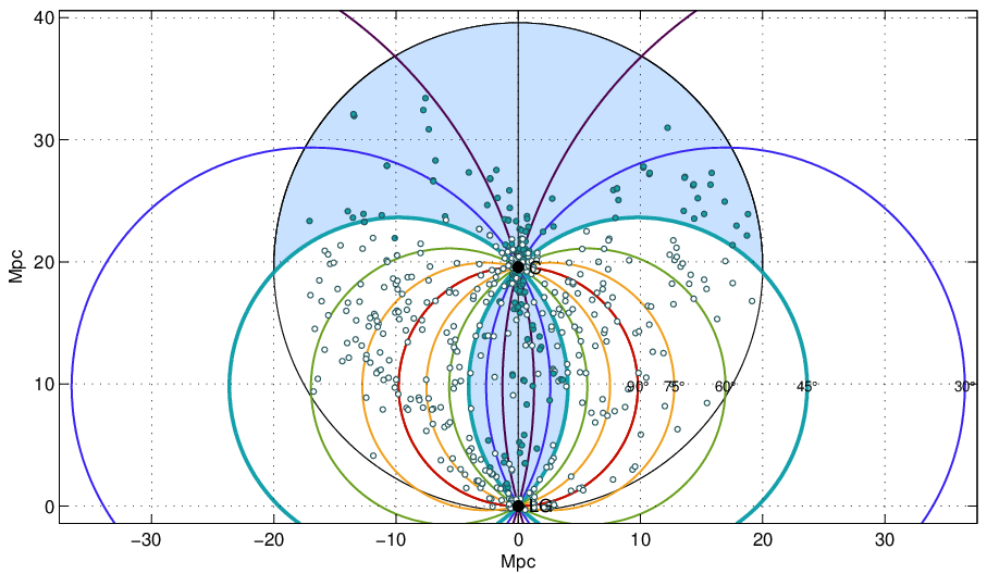
Finally, in order to reduce the role of the unknown tangential component of the velocity and to avoid further uncertainties, we decided to select for our analysis only galaxies situated approximately in front and behind the cluster, i.e. in a cone satisfying the conditions or . The number of galaxies satisfying this additional constraint within 20 Mpc of the Fornax center is 164 and their projected distribution in the sky is shown in Figure 4.
It should be mentioned that the role of possible chaotic tangential velocities of the galaxies had been studied by Karachentsev & Kashibadze (2006). They have performed numerical simulations, adding some random tangential component to the observed radial velocity. Their modeling of the Hubble flow in the vicinity of the Local Group showed that typical tangential velocities with amplitudes of 35 and 70 km s-1 produce a statistical uncertainty in the evaluation of the zero-velocity surface radius as small as 2% and 4% respectively.
3 Mass estimates
The difficulties with the different mass estimators were already mentioned. In particular, the presence of interlopers lead to an overestimate of the mass ranging from 10% up to 60% when the virial relation is used, whereas estimates based on X-ray data have uncertainties ranging from 14–30%.

The case of the Fornax cluster is quite particular. Unlike clusters as Coma or Virgo, which have a well defined center and a more or less smooth mass distribution, despite the presence of some substructures, the Fornax cluster has a complicated mass distribution, including many substructures. Such a complexity is sketched in Figure 5 where it is possible to identify: the Fornax cluster centered on NGC 1399, the Eridanus subcluster, including the groups NGC 1407, NGC 1332, NGC 1395 and NGC 1398 as well as other small neighboring groups. It should be emphasized that the virial radii of these groups do not overlap, suggesting that these objects are separated and constitute gravitationally bound structures. However these groups overlap in the scale of the zero-velocity radius, indicating that despite the absence of dynamical equilibrium, they are probably bound to the main structure.
3.1 The spatial position of the Fornax-Eridanus barycenter
| Group | RA, Dec | |||||||||||||||
|---|---|---|---|---|---|---|---|---|---|---|---|---|---|---|---|---|
| hh mm ss dd mm ss | km/s | km/s | kpc | Mpc | Mpc | ∘ | ∘ | ∘ | ∘ | |||||||
| (1) | (2) | (3) | (4) | (5) | (6) | (7) | (8) | (9) | (10) | (11) | (12) | (13) | (14) | (15) | (16) | (17) |
| NGC 1097 | 024621.0314430 | 4 | 1 | 1189 | 81 | 140 | 43 | 11.26 | 12.53 | 15.9 | 3.2 | 16.3 | 11 | 131 | 10 | 142 |
| NGC 1187 | 030238.6230819 | 4 | 1 | 1315 | 28 | 48 | 106 | 10.60 | 11.90 | 18.4 | 3.7 | 18.0 | 15 | 96 | 9 | 125 |
| NGC 1201 | 030408.0275549 | 2 | 2 | 1633 | 48 | 48 | 312 | 10.95 | 11.94 | 21.0 | 0.8 | 22.4 | 12 | 65 | 7 | 88 |
| NGC 1232 | 030945.5212514 | 3 | 2 | 1582 | 49 | 70 | 475 | 11.07 | 12.93 | 19.2 | 0.5 | 21.7 | 16 | 86 | 10 | 113 |
| NGC 1291 | 031718.6425331 | 3 | 3 | 703 | 70 | 99 | 226 | 11.03 | 13.09 | 8.2 | 0.5 | 9.6 | 6 | 170 | 13 | 159 |
| NGC 1302 | 031723.8260702 | 6 | 4 | 1663 | 21 | 47 | 383 | 11.15 | 12.30 | 19.2 | 1.0 | 22.8 | 10 | 91 | 5 | 136 |
| NGC 1332 | 032500.7212102 | 22 | 9 | 1469 | 40 | 183 | 279 | 11.55 | 13.39 | 24.1 | 0.8 | 20.1 | 15 | 45 | 8 | 43 |
| NGC 1340 | 032819.7325555 | 3 | 2 | 1074 | 4 | 6 | 432 | 10.73 | 11.76 | 20.2 | 0.4 | 14.7 | 5 | 67 | 3 | 131 |
| NGC 1399 | 033230.3360845 | 111 | 79 | 1411 | 23 | 244 | 454 | 12.30 | 13.94 | 19.6 | 0.2 | 19.3 | 0 | 0 | 7 | 116 |
| IC 1970 | 033631.5440235 | 2 | 1 | 1090 | 9 | 9 | 103 | 10.06 | 10.06 | 19.4 | 2.0 | 14.9 | 8 | 90 | 15 | 99 |
| NGC 1386 | 033734.3360610 | 8 | 5 | 755 | 26 | 70 | 165 | 10.37 | 12.40 | 19.8 | 0.9 | 10.3 | 1 | 58 | 7 | 113 |
| NGC 1398 | 033754.9260905 | 10 | 4 | 1386 | 30 | 89 | 612 | 11.46 | 13.09 | 22.7 | 1.8 | 19.0 | 10 | 45 | 3 | 34 |
| NGC 1407 | 034002.6191705 | 25 | 5 | 1713 | 34 | 167 | 385 | 11.61 | 13.22 | 24.2 | 1.2 | 23.5 | 17 | 47 | 10 | 47 |
| NGC 1395 | 034014.0231718 | 24 | 11 | 1548 | 25 | 121 | 378 | 11.53 | 13.05 | 24.3 | 1.0 | 21.2 | 13 | 41 | 6 | 34 |
| NGC 1482 | 035438.9212951 | 3 | 2 | 1715 | 55 | 78 | 48 | 10.70 | 11.32 | 28.9 | 3.1 | 23.5 | 16 | 28 | 9 | 23 |
| NGC 1519 | 040703.1183633 | 4 | 2 | 1781 | 15 | 26 | 238 | 10.29 | 11.57 | 23.8 | 2.4 | 24.4 | 20 | 51 | 14 | 56 |
| NGC 1532 | 041226.4332640 | 10 | 3 | 1159 | 30 | 89 | 137 | 11.25 | 12.70 | 20.3 | 1.5 | 15.9 | 9 | 72 | 9 | 98 |
In the present paper we regard the dynamical center of the Fornax cluster (NGC 1399 group) situated near the core of the hot X-ray emitting gas (Jones et al. 1997, Scharf et al. 2005, Machacek et al. 2005) as the gravity center of the whole Fornax-Eridanus complex. Its spatial position was calculated as the mean position of all NGC 1399 group members, yielding Mpc, and . For the moment this choice (as the first approximation) seems to be reasonable since the NGC 1399 region has been investigated most detaily. The next step is to determine the spatial position of the Fornax-Eridanus complex barycenter as the weighted mean for position vectors of all the virialized substructures forming the complex. This will be possible after obtaining more observational data in a wider area of the complex. Still, the same calculation techniques are applied by us for both center positions (with values Mpc, , adopted for the second case), and the resulting values didn’t differ significantly. The barycenter position associated with NGC 1399 group yields 0.23 Mpc lower value from precise data and 0.19 Mpc higher value from Tully-Fisher data, leading to the upper bound of discrepancy Mpc. Generally speaking, the zero-velocity surface method is rather stable in the sense of a barycenter position (Karachentsev & Kashibadze 2006).
Table 2 represents groups, triplets and pairs forming the Fornax-Eridanus complex with individual distance estimates (Karachentsev & Makarov 2008; Makarov & Karachentsev 2009, 2011). Columns of the table contain: (1) name of the brightest galaxy in a group/triplet/pair; (2) equatorial coordinates of the brightest galaxy for triplets and pairs or mean equatorial coordinates for groups (at the J2000.0 equinox); (3) number of galaxies in a system; (4) number of galaxies with measured distances; (5, 6) mean velocity with respect to the Local Group centroid and its error; (7) radial velocity dispersion; (8) harmonical radius; (9) integrated luminosity of the group in the band; (10) virial mass of the group; (11, 12) mean distance of the group and its error; (13) Hubble distance calculated as where km s-1 Mpc-1; (14) and (16) angular distance to the Fornax-Eridanus complex barycenter for the cases of (14) dynamical center of the NGC 1399 group situated near the center of the hot X-ray emitting gas and (16) dynamical center of all substructures forming the complex; (15) and (17) angle between the directions to the Local Group and to the Fornax-Eridanus complex barycenter for both cases mentioned above, respectively.
The possible role of barycenter position is illustrated by Figure 6 representing velocity vs. distance diagrams where only the centers of the groups forming the Fornax-Eridanus complex are shown. The top panel represents radial velocities and distances of the groups relative to the Local Group centroid. The distance to the Fornax-Eridanus complex, 21.1 Mpc, corresponds to the spatial position of the complex barycenter as the weighted mean for position vectors of all the virialized substructures forming the complex. The sets of dashed and dotted lines indicate the Hubble flow perturbed by a point-like mass of and respectively which corresponds to the mass of the whole Fornax-Eridanus complex estimated in this paper and the virial mass estimation of the Fornax cluster itself (Makarov & Karachentsev 2011). Both sets include S-shaped lines signing different angular separations from the complex center (, , and ). The error bars indicate rms uncertainties in distances and velocities.
The velocity vs. distance diagram relative to the center of the Fornax-Eridanus complex is shown in the bottom panel of the Figure 6. Two types of markers, circles and squares, correspond to the center of the hot X-ray emitting gas and the dynamical center of all substructures forming the complex, respectively. The solid line indicates the Hubble flow perturbed by a point-like mass of (the virial mass estimation of the Fornax cluster itself) while the dashed and dotted lines are constructed as least square estimates for both adopted center positions mentioned above ( and respectively).


The structural complexity of the galaxy distribution suggests that probably the best mass indicator for this cluster should be based on the velocity field of the outskirt galaxies. Here two approaches will be adopted. In the first, the radius of the zero velocity surface will be estimated from a running median procedure. From the knowledge of , the mass inside such a surface follows immediately. In the second, the expected radial velocity profile derived from the spherical model is fitted to the data and again, the mass inside the zero-velocity surface results from the derived fit parameters.
3.2 The running median
The zero-velocity radius can be estimated from a running median procedure, using directly observational data (Figure 7).


In order to account errors in observed distances and velocities and to give some estimates of the uncertainties, a Monte-Carlo simulations technique was used. For any galaxy in a given dataset , a corresponding distance from the center is generated according to the relation , where is the observed distance from the Fornax center, is an observational error associated to the distance and is a normally distributed random number (with ). Generated velocities were derived by a similar procedure. About 10,000 datasets were generated and for each of them the running median method was applied, yielding different values of , which were then averaged. The distribution of 10,000 are shown in Figure 8 as well as the mean and median values and the 90 %error band (for the window Mpc). The resulting median values and corresponding errors for (A) minor attractor and (B) major extended attractor cases are given in Table 3. The first two columns correspond to the cases when only precise or Tully-Fisher data were used for Monte-Carlo simulations while the third column corresponds to the whole dataset. The lines of the table correspond to the different median windows.

| Window | Precise distances | TF distances | All | |||
|---|---|---|---|---|---|---|
| (Mpc) | (samples 1–4) | (samples 5–6) | samples | |||
| (A) | (B) | (A) | (B) | (A) | (B) | |
| 0.8 | 4.48 | 4.56 | 4.87 | 5.15 | 4.41 | 4.67 |
| 3.885.46 | 3.945.63 | 3.956.18 | 4.086.68 | 3.835.39 | 3.935.76 | |
| 1.0 | 4.58 | 4.72 | 5.04 | 5.39 | 4.42 | 4.78 |
| 3.875.50 | 3.955.75 | 3.956.32 | 4.096.81 | 3.825.42 | 3.935.79 | |
| 1.2 | 4.51 | 4.66 | 5.15 | 5.51 | 4.39 | 4.83 |
| 3.885.56 | 3.925.85 | 3.956.33 | 4.166.86 | 3.825.48 | 3.935.88 | |
With the Fornax cluster distance of Mpc and the typical uncertainty of 10 % for the ACSFCS+ galaxies populating the central core of the cluster, the observational distance errors in the virialized zone will be of about 2 Mpc. Assuming the virial radius of the Fornax cluster to be Mpc we should conclude that the cluster core galaxies can possibly distort the pattern in the region for the Fornax cluster itself, but not for the whole Fornax-Eridanus complex. Anyway, the galaxies in the Fornax cluster core, i.e. those with Mpc, were not regarded in the Monte-Carlo data simulations, resulting to 109 galaxies (see Figure 7).
The substantial dip in the running median of simulations based on precise data can be explained partially by the enormous velocity of NGC 1400 (see, for example, Perrett et al. 1997). Belonging to the NGC 1407 group, NGC 1400 has an extremely low velocity relative to the Local Group (558 km s-1) while NGC 1407 has km s-1. Both galaxies have roughly the same distance (26.4 Mpc for NGC 1400 and 28.8 Mpc for NGC 1407 according to Tonry et al. 2001). In the velocity-distance diagrams NGC 1400 has a significant negative velocity relatively to the Fornax-Eridanus complex center, 380 km s-1 and 988 km s-1 for the cases of minor and major attractors respectively, and therefore it appears in the legend region at the Fornax-centric distance of 9.6 Mpc shifting the running median downwards.
According to the Table 3, the median estimate of is 4.60 Mpc with confidence interval corresponding to 90 % error band of Mpc.
Once is known, the mass inside the zero-velocity surface can be computed. Using the spherical model, including the effects of the cosmological constant, the mass inside is (E. Shaya, private communication; Karachentsev et al. 2007)
| (1) |
where
| (2) |
with being the mass density parameter.
Figure 9 shows the ratio of masses of a galaxy system computed in the CDM model and in the empty Universe model respectively as a function of . As one can see, the adopted uncertainty in value affects as about 3 % in mass estimation, which is negligible as compared with uncertainties caused by observational errors.

CDM parameters can be determined from WMAP data with a sufficient accuracy, i.e., km s-1 Mpc-1 and (Spergel et al. 2007). Substituting these values into the Equation (1), we get
| (3) |
Notice that from the numerical solution of the equations describing the Lemaître-Tolman model, modified in order to include effects of the cosmological constant, Peirani & de Freitas Pacheco (2008) obtained for the mass inside the zero-velocity surface
| (4) |
The numerical coefficient was obtained for and for both relations derived either analytically or numerically agree quite well. For = 4.60 Mpc the corresponding total mass of the Fornax complex is and for the limiting values of 90 % error band Mpc we obtain as a confidence interval.
3.3 Mass estimate from the radial velocity profile
In this section, the mass inside the zero-velocity surface is estimated by fitting a theoretical profile directly to data. We follow the procedure developed by Peirani & de Freitas Pacheco (2006, 2008), who have numerically computed the velocity field of outskirt galaxies, based on the spherical collapse model including effects of the cosmological constant. This approach assumes that: a) most of the cluster mass is concentrated in the core, in which the shell crossing has already occurred and b) that orbits of galaxies outside the core are mainly radial. From the numerical calculations by Peirani & de Freitas Pacheco (2008), the velocity-distance relation is
| (5) |
Here is the core cluster mass, is the distance of the member galaxy to the cluster center, is the radial velocity of the galaxy with respect to the mass center, is the present value of the Hubble parameter and . The relation above results from a fit of numerical data and is valid for the present time (), since it varies as a function of the redshift. Notice that eq. 4 can be deduced from this equation when .


In principle, if accurate radial velocities and distances are available, from the fitting of eq. 5 to data it is possible to derive both the core cluster mass and the Hubble parameter (Peirani & de Freitas Pacheco 2008). Here face to the uncertainties in the determination of Fornax-centric velocities, as explained in the previous section, we adopted the procedure of fixing as 73 km s-1 Mpc-1 and computing the mass either for the “minor attractor” or for the “major extended attractor” models.
| Parameter | “Minor attractor” | “Major attractor” |
|---|---|---|
| Mass (in | 0.93 | 1.55 |
| 0.382.10 | 0.434.54 | |
| (in Mpc) | 3.44 | 4.08 |
| 2.574.52 | 2.675.85 | |
| (in km s-1) | 300 | 345 |
| (in km s-1) | 84 | 190 |
Masses resulting from our fitting procedure are given in Table 4 for the two models adopted to estimate Fornax-centric velocities. The zero velocity surface radius and the velocity dispersion with respect to the mean infall flow are also given. The second column corresponds to velocities estimated from the “minor attractor” approach whereas the third column gives values derived from the “major extended attractor” model. The corresponding confidence intervals for mass and values are estimated as 90 % error band. The third and the fourth lines give respectively the uncorrected and the corrected velocity dispersions with respect to the infall flow towards Fornax. Notice that this method leads to values of masses that are, on the average, 50% smaller than the “running median” approach, being rather a mass estimate for the Fornax cluster core than for the total Fornax-Eridanus complex. It is worth mentioning that the derived 1-D velocity dispersion with respect the bulk motion, (300–345 km s-1), is one order of magnitude higher than that observed in the vicinities of the Local Group but it drops to (84–190 km s-1) when the distance measurement errors are taken into account. Figure 10 shows the best fit between the expected velocity profile (eq. 5) derived from the spherical model and data, whose velocities were computed according to the “minor attractor” model (upper panel) or to the “major attractor” model (lower panel). The number of galaxies used in the fitting procedure is limited by satisfying the relation and actually accounts for 22 and 23 galaxies respectively.
Considering the mass values estimated from these procedures we adopt for the Fornax cluster itself a mass of with the confidence interval of , and for the total Fornax-Eridanus complex a mass of with the confidence interval of , which corresponds to a value half order of magnitude the Virgo cluster mass. In Table 5 we compare previous mass estimates for the Fornax cluster (normalized to Mpc and Mpc) with the present study, based on the velocity field of outskirt galaxies.
| Fornax | Eridanus | Other clumps | Total | Reference |
| 1.53 | 0.20 | 0.15 | 1.88 | 1 |
| 1.15 | 0.70 | 1.85 | 2 | |
| 0.7 | 3 | |||
| 1.00 | 0.92 | 1.92 | 4 | |
| 0.87 | 0.62 | 0.43 | 1.92 | 5 |
| 0.403.32 | 6, eq. 5 | |||
| 1.303.93 | 6, via |
4 Concluding remarks
The distribution of galaxies in the vicinity of the Fornax cluster indicates a substantial degree of subclustering that forming the Fornax complex. As a consequence, mass estimates based on the virial relation are affected by the fact that the system has not yet reached an equilibrium state and is still probably in formation (Dunn & Jerjen 2006). In fact dwarf galaxies have distinct dynamic properties in comparison with bright galaxies and are probably infalling into the system (Drinkwater et al. 2001). These difficulties may be circumvent by studying the velocity field of outskirt galaxies, which permits an estimate of the zero-velocity surface and, consequently of the mass inside such a surface as proposed originally by Lynden-Bell (1981) and Sandage (1986).
In this investigation, a culled sample of 109 galaxies with measured distances and within 20 Mpc from the cluster center were used to study the velocity field in the neighborhood of the Fornax cluster. Since tangential velocities are unknown, in order to estimated the galaxy velocities with respect to the cluster center two main assumptions were made: in the first, it was supposed that the velocity vector is essentially dominated by the Hubble flow (“minor attractor" model) while in the second, it was assumed that galaxies are infalling radially (“major attractor" model). The zero-velocity radius was derived by two different methods: the “running median" and by fitting directly the data to the expected velocity profile derived from the spherical model, including the effects of a cosmological constant.
The best fit radius of the zero-velocity sphere for the Fornax-Eridanus complex is estimated by us to be Mpc with the confidence interval of Mpc while the mass inside such a surface is . At the distance to Fornax cluster 20 Mpc, the radius Mpc corresponds to shown in Figure 5. Notice that within this circle there are almost all systems identified by Makarov & Karachentsev (2011) as virialized groups bound to Fornax cluster. Their total virial mass, , agrees with , meaning that probably only a small part of the Fornax-Eridanus complex mass is spreaded between the groups.
Acknowledgements.
Support of this work has been provided by Henri Poincaré Junior Fellowship of ADION in 2010, Observatoire de la Côte d’Azur, CNRS, France; the Dynasty Foundation of Noncommercial Programs, Russia; The Ministry of Education and Science of the Russian Federation (contract no. 14.740.11.0901); the Russian Foundation for Basic Research (projects no. 10-02-92650, 11-02-00639).References
- (1) Biviano A., Murante G., Borgani S. et al. 2006, A&A, 456, 23
- (2) Blakeslee J. P., Jordán A., Mei S. et al. 2009, ApJ, 694, 556
- (3) Broadhurst T. J., Taylor A. N., Peacock J. A. 1995, ApJ, 438, 49
- (4) Brough S., Forbes D. A., Kilborn V. A. et al. 2006, MNRAS, 369, 1351
- (5) Crook A. C., Huchra J. P., Martimbeau N. et al. 2007, ApJ, 655, 790
- (6) Danese L., de Zotti G., Giuricin G. et al. 1981, ApJ, 244, 777
- (7) Diaferio A. 1999, MNRAS, 309, 610
- (8) Drinkwater M. J., Gregg M. D., Holman B. A., Brown M. J. I. 2001, MNRAS, 326, 1076
- (9) Dunn L. P. & Jerjen H. 2006, AJ, 132, 1384
- (10) Evrard A. E., Croton D., White M., Cohn J., Ellingson E. 2006, BAAS, 38, 1196
- (11) Ferguson H. C. 1989, AJ, 98, 367
- (12) Ferguson H. C. & Sandage A. 1990, AJ, 100, 1
- (13) Fernley J. A. & Bhavsar S. P. 1984, MNRAS, 210, 883
- (14) Girardi M. & Biviano A. 2002, in Merging Processes in Galaxy Clusters, eds. L. Ferreti, I. M. Gioia and G. Giovannini, Dordrecht, Kluwer, p. 39
- (15) Haynes M. P., Giovanelli R., Salzer J. J. et al. 1999 AJ, 117, 1668
- (16) Jerjen H. 2003, A&A, 398, 63
- (17) Jones C., Stern C., Forman W. et al. 1997, ApJ, 482, 143
- (18) Karachentsev I. D. & Makarov D. I. 1996, AJ, 111, 794
- (19) Karachentsev I. D., Sharina M. E., Makarov D. I. et al. 2002a, A&A, 389, 812
- (20) Karachentsev I. D., Dolphin A. E., Geisler D. et al. 2002b, A&A, 383, 125
- (21) Karachentsev I. D., Karachentseva V. E., Huchtmeier W. K., Makarov D. I. 2004, AJ, 127, 2031 (CNG)
- (22) Karachentsev I. D. & Kashibadze O. G. 2006, Astrophysics, 49, 3
- (23) Karachentsev I. D., Dolphin A. E., Tully R. B. et al. 2006, AJ, 131, 1361
- (24) Karachentsev I. D., Tully R. B., Dolphin A. E. et al. 2007, AJ, 133, 504
- (25) Karachentsev I. D. & Makarov D. I. 2008, AstBu, 63, 299
- (26) Karachentsev I. D., Kashibadze O. G., Makarov D. I., Tully R. B. 2009, MNRAS, 393, 1265
- (27) Karachentsev I. D. & Nasonova O. G. 2010, MNRAS, 405, 1075
- (28) Kashibadze O. G. 2008, Astrophysics, 51, 409
- (29) Koribalski B. S., Staveley-Smith L., Kilborn V. A. et al. 2004, AJ, 128, 16
- (30) Kudrya Yu. N., Karachentseva V. E., Karachentsev I. D. et al. 2003, A&A, 407, 889
- (31) Lynden-Bell D. 1981, The Observatory, 101, 111
- (32) Machacek M., Dosaj A., Forman W. et al. 2005, ApJ, 621, 663
- (33) Makarov D. I. & Karachentsev I. D. 2009, AstBu, 64, 24
- (34) Makarov D. I. & Karachentsev I. D. 2011, submitted to MNRAS
- (35) Mellier Y. 1999, ARA&A, 37, 127
- (36) Methewson D. S., Ford V. L. 1996, ApJS, 107, 97
- (37) Metzler C. A., White M., Norman M., Loken C. 1999, ApJ, 520, L9
- (38) Mitronova S. N., Karachentsev I. D., Karachentseva V. E., Jarrett T. H., Kudrya Yu. N. 2004, Bull. Spec. Astrophys. Obs., 57, 5 (2MFGC)
- (39) Peebles P. J. E. 2005, personal communication
- (40) Peirani S., de Freitas Pacheco J. A. 2006, New Astron., 11, 325
- (41) Peirani S., de Freitas Pacheco J. A. 2008, A&A, 488, 845
- (42) Perea J., del Olmo A., Moles M. 1990, A&A, 237, 319
- (43) Perrett K. M., Hanes D. A., Butterworth S. T. et al. 1997, AJ, 113, 895
- (44) Regos E. & Geller M. J. 1989, AJ, 98, 755
- (45) Reiprich T. H. & Bohringer H. 2002, ApJ, 567, 716
- (46) Rizzi L., Tully R. B., Makarov D. I. et al. 2007, ApJ, 661, 813
- (47) Rosati P., Borgani S., Norman C. 2002, ARA&A, 40, 539
- (48) Sandage A. 1986, ApJ, 307, 1
- (49) Sarazin C. L. 1986, Rev. Mod. Phys., 58, 1
- (50) Scharf C. A., Zurek D. R., Bureau M. 2005, ApJ, 633, 154
- (51) Spergel D. N.; Bean R.; Doré O. et al. 2007, ApJS, 170, 377.
- (52) Springob C. M., Haynes M. P., Giovanelli R., Kent B. R. 2005, ApJS, 160, 149
- (53) Springob C. M., Masters K. L., Haynes M. P. et al. 2007, ApJS, 172, 599
- (54) Theureau G., Martin J. M., Cognard L. et al. 2006, in ASP conference ser., Vol. 351, ed. G. Gabriel, p. 429
- (55) Tifft W. G. & Huchtmeier W. K. 1990, A&AS, 84, 47
- (56) Tonry J. L., Dressler A., Blakeslee J. P. et al. 2001, ApJ, 546, 681
- (57) Tonry J. L., Schmidt B. P., Barris B. et al. 2003, ApJ, 594, 1
- (58) Tully R. B. 1987, ApJ, 321, 280
- (59) Tully R. B., Pierce M.J. 2000, ApJ, 533, 744
- (60) Tully R. B., Rizzi L., Dolphin A. E. et al. 2006, AJ, 132, 729
- (61) Tully R. B., Shaya E. J., Karachentsev I. D. et al. 2008, ApJ, 676, 184
- (62) Tully R. B., Rizzi L., Shaya E. J. et al. 2009, AJ, 138, 323
- (63) Voit G. M. 2005, Rev. Mod. Phys., 77, 207
- (64) Wu X.-P., 2000, MNRAS, 316, 29