Chameleon stars
Abstract
We consider a gravitating spherically symmetric configuration consisting of a scalar field non-minimally coupled to ordinary matter in the form of a perfect fluid. For this system we find static, regular, asymptotically flat solutions for both relativistic and non-relativistic cases. It is shown that the presence of the non-minimal interaction leads to substantial changes both in the radial matter distribution of the star and in the star’s total mass. A simple stability test indicates that, for the choice of parameters used in the paper, the solutions are unstable.
I Introduction
In cosmology scalar fields play a key role in models of both the inflation era of the early Universe [1] and the current accelerated expansion [2]. Scalar fields are also widely used to study smaller scale objects such as the effect of a dark matter, scalar field on the structure of galaxies [3]. Moving to still smaller scales there have been studies of boson stars [4] – compact (usually spherically symmetric) configurations formed from gravitating scalar field(s). The sizes of such configurations varies from the microscopic (“gravitational atom”) up to sizes corresponding to massive black holes such as those presumed to exist at the center of many galaxies including our own. In this connection, it is quite natural to investigate the role that such scalar fields may have in the processes of formation and evolution of galaxies and more compact astrophysical structure – stars and their clusters. As applied to the stars, it is possible to imagine a situation where scalar fields can exist inside usual stars consisting of ordinary matter. The existence of such scalar fields would undoubtedly have an impact on the star’s inner structure. One such example is the model of a star consisting of both ordinary polytropic matter and a ghost scalar field [5]. The presence of the field leads to the appearance of a tunnel at the center of such stellar configurations which provides new geometric and physical properties to such objects. Another example of such stellar objects involves fermion fields interacting with a real scalar field not only gravitationally but also through the Yukawa coupling of the type , where is a Yukawa type coupling constant [6]. Further examples of mixed configurations consisting of both boson and fermion fields can be found in references [7, 8, 9].
The investigation in the present work is along the direction of the above works – we consider a scalar field interacting non-minimally with ordinary matter in the form of a perfect polytropic fluid. An interaction similar to this was used to describe the evolution of dark energy within the framework of chameleon cosmologies [10, 11]. In chameleon cosmologies the properties of the scalar (chameleon) field depend strongly on the environment [12] into which it is embedded. For example, the mass of the scalar field can change depending on the background environment [12]. As will be shown below, the presence of such an interaction between the polytropic fluid and the scalar field results in a substantial change of the inner structure of the polytropic star. This change is related to the fact that the behavior of the scalar field depends the “environment” (i.e. the fluid) into which it is embedded as is the case with chameleon cosmology models. Thus we call these configurations chameleon stars.
In building our model of a chameleon star we will use a real scalar field. In the bulk of the literature complex (charged) scalar fields are more often used in constructing models of boson stars. The charge of the complex scalar field generically leads to repulsion which counteracts the attraction of gravity and thus gives a physical basis for the existence of these boson star solutions. Real scalar fields have received less attention because they do not carry a charge, and constructing regular stable solutions is more difficult task in this case. The known static solutions for real scalar fields are either singular [13, 14], or use phantom scalar fields [15, 16, 17]. Singular solutions with trivial topology and non-phantom fields have been found for both massless fields [13] and for self-interacting fields [14]. The latter ordinary scalar field solutions are asymptotically flat but the issue of their stability is not quite clear (for further discussion see reference [18]). In [19] regular, static solutions in the presence of the cosmological constant were found. In this case the space-time asymptotically approaches de Sitter space-time. The linear stability analysis of these solutions indicate that they are unstable. In contrast the paper [20] found regular, static solutions which asymptotically approached anti-de-Sitter space-time, which were stable under a linear stability analysis. In the present paper the real scalar field non-minimally interacts with the polytropic fluid. As will be shown below, this leads to the existence of regular, asymptotically flat solutions.
In the absence of gravity, Derrick’s theorem [21, 22] forbids the existence of non-trivial, stable, regular static dimensional solutions from only scalar fields. This theorem assumes that the potential energy of the system is some non-negative function, , vanishing only at its absolute minima. A partial extension of Derrick’s theorem to the case of general relativity has been studied in [23, 24] where it was shown that the existence of asymptotically flat particle-like solutions with a regular center and normal (non-phantom) scalar fields is also impossible if . The distinction between the non-gravitational form of Derrick’s theorem [21, 22] and the gravitational variant [23, 24] is that the latter does not touch on the stability of the solutions.
If one allows other fields besides just scalar fields (e.g. vector or fermion fields) then there are static solutions when the spatial dimensionality is three or more. In the absence of gravity, one has the ’t Hooft-Polyakov monopole which is a finite energy, stable solution for Yang-Mills vector fields plus scalar fields [25, 26]. In the presence of gravity plus a real scalar field there are boson star solutions (for a review see [4]) which however have one or more of the bad features listed above (e.g. non-trivial topology, not asymptotically flat, not stable)
In this paper we study the gravitating system of a real scalar field plus a perfect fluid and show that for this system there are regular, three-dimensional, static solutions. The most important feature of this system, aside from the gravitational interaction, is the presence of the non-minimal coupling between the scalar field and the perfect fluid. It is this interaction which allows us to avoid the restrictions of the gravitational version of Derrick’s theorem [23, 24], and find regular static solutions even if the potential energy of the scalar field satisfies . We take a polytropic equation of state for the perfect fluid. Stellar models using polytropic fluids were investigated in detail both within the framework of Newtonian gravitational theory [27] and for strong gravitational fields [28]. Both of these studies hinted at the existence of finite size, regular solutions. These solutions were successfully used to give a description of both non-relativistic stars and stars where relativistic effects were important e.g. neutron stars. As will be shown below, the inclusion of the non-minimal interaction between the polytropic fluid and the scalar field leads to regular solutions which, however, are generally different from usual polytropic stars.
The paper is organized as follows: In section II the general equations describing a static configuration consisting of a real scalar field coupled to a perfect polytropic fluid are derived. In section III these equations are written for a particular case when the potential energy of the scalar field is chosen to have a quadratic mass term and a quartic self-interaction term. For this potential energy, in section IV we give the results of the numerical calculations for this potential for both relativistic and non-relativistic cases, and discuss the issue of the stability of the solutions obtained. Next, in section V we present a simple analytical solution for the non-relativistic case with the scalar field taken to be massless and for a special choice of the coupling function. Finally, in section VI we summarize the main results and give some speculations about the physical applications of these chameleon star configurations to neutron stars and living stars (i.e. stars still on the main sequence).
II Derivation of equations for a static configuration
As discussed in the introduction we consider a gravitating system of a real scalar field coupled to a perfect fluid. The Lagrangian for this system is
| (1) |
Here is the real scalar field with the potential ; is the Lagrangian of the perfect isotropic fluid i.e. a fluid with only one radial pressure; is some function describing the non-minimal interaction between the fluid and the scalar field. The case corresponds to the absence of the non-minimal coupling, but even in this case the two sources are still coupled via gravity.
We choose the Lagrangian for the isentropic perfect fluid to have the form [29, 30]. Using this Lagrangian, the corresponding energy-momentum tensor is (details are given in Appendix A)
| (2) |
where and are the density and the pressure of the fluid, is the four-velocity (here and throughout the paper we set ). We take the static metric of the form
| (3) |
where is the metric on the unit 2-sphere. The and components of the Einstein equations for the metric (3) and the energy-momentum tensor (2) are
| (4) | |||
| (5) |
The equation for the scalar field coming from the Lagrangian (1) is
Using this field equation above with the perfect fluid , and the metric (3), gives the following scalar field equation
| (6) |
where the prime denotes differentiation with respect to . The Einstein field equations are not all independent because of the relation . The component of this equation has the form
| (7) |
Taking into account the expressions
and , from (4), (5) and using (6), allows us to write (7) as
| (8) |
The matter Lagrangian used here, , is not the only possibility. Other variants can be found in [31]. However, the choice has the simplifying feature (8) does not contain additional terms involving the coupling function .
For a polytropic equation of state one has
| (9) |
where are constants. Now one can introduce the new variable defined as [32]
| (10) |
Here is the central density, and the constant , the polytropic index, is related to via . Putting these definitions together gives equation (9) in the form
| (11) |
Using (11) in equation (8) leads to
| (12) |
with and is the pressure of the fluid at the center of the configuration. This equation may be integrated to give in terms of :
| (13) |
where is the value of at the center of the configuration where . The integration constant , corresponds to the value of at the center of the configuration. It is determined by requiring at infinity that i.e. that the space-time is asymptotically flat.
The gravitating system of a real scalar field interacting with a perfect fluid is characterized by three unknown functions – and . These three functions are determined by the three equations (4), (5) and (6), and also by the relation (13). We now rewrite these equations by the introduction of a new function [28]
| (14) |
Here is the mass of the configuration within the range , where is the boundary of the fluid where . Using this function, equation (4) becomes
| (15) |
From (14) one can define which can be interpreted as the total mass of the configuration in the range . This mass has contributions from both the fluid and the scalar field, within a sphere of coordinate radius . To avoid a singularity in at the origin, one has to put [28]. This corresponds to the fact that the mass at the origin is equal to zero i.e. .
In anticipation of analyzing the system of equations – (4), (5) and (6)) – numerically, we introduce the following dimensionless variables
| (16) |
has the dimensions of an inverse length. With this one can rewrite equations (4) and (5) in the form
| (17) | |||||
| (18) |
where is the dimensionless potential energy of the field.
III Configuration with a mass and a quartic self-interaction term
In this section we will show that there are non-singular, finite-mass solutions of equations (17)-(19). First we specify the boundary conditions. Using the above dimensionless variables we “normalize” to unity at the center of the configuration
| (20) |
From equation (17) one can show that like as . Combining this with equation (18) one in turn finds as . Bearing in mind that we are looking for regular solutions, we define the boundary conditions in the vicinity of as
| (21) |
where corresponds to the initial value of the scalar field , the parameters are arbitrary, and the value of the coefficient is defined from equation (19) as
The index denotes that the values of the functions are taken at .
Using the boundary conditions (21), we proceed to solve the system (17)-(19) numerically. The behavior of the solution will depend both on the parameters of the polytropic fluid and the form of the potential energy of the scalar field , and the coupling function . One of the simplest and most commonly used choices for the potential energy is that of a scalar field with mass and a quartic self-interaction term ()
It was pointed out in [14] that the system with such potential has only singular static solutions. Below we show that an inclusion of the non-minimal interaction between the scalar field and the polytropic fluid allows one to obtain regular static solutions. As an example, let us choose the coupling function in dimensionless form as follows
| (22) |
Then, using the dimensionless variables introduced in the previous section, the potential can be rewritten as
| (23) |
where the new dimensionless constants are given as
Using the above potential and the function , equations (17)-(19) take the form
| (24) | |||||
| (25) | |||||
| (26) | |||||
The parameter can be absorbed by introducing the rescalings , , , . Bearing this in mind, we assume in further calculations. One can see from these equations that the presence of the interaction between the scalar field and the fluid is defined by the parameter . In the absence of the fluid, this system only has singular solutions [14]. The inclusion of the fluid changes the situation since the presence of the term on the right hand side of (26) for the scalar field corresponds to an effective mass term whose sign depends both on the behavior of the fluid density and the values of the parameters and . We note that the present system of gravitating real scalar field plus perfect fluid turns out to be similar to the gravitating complex scalar scalar field system considered in [33]. The gravitating complex scalar field studied in [33] had a potential of the type (23) and it gave regular, stationary solutions. Thus this is already a hint that we can expect regular, stationary solutions for the present system.
IV Numerical results
IV.1 Relativistic case
The results of the numerical calculations for the system (24)-(26) with the boundary conditions (21) are presented in tables 1 and 2. The solutions were started near the origin (i.e. near ) and solved out to a point where the function becomes zero. From equations (9) and (10) this is where the fluid vanishes and it is this point, , that we define to be the surface of the star. Beyond the point we continued the numerical solutions with only the gravitational and scalar fields while the fluid was set to zero. The interior and exterior solutions were then connected to one another. Details of this are given below. Previous numerical studies with a fluid having a polytropic equation of state [28] found regular, relativistic star-like configurations. These star-like solutions of [28] where found for the values of the parameters and . Since our system has two additional parameters () we restrict ourselves to examine just two sets of the parameters (i.e. and ) at different values of and when looking for regular solutions. Below we show that these two sets of solutions differ considerably in the behavior of their physical characteristics.
The parameters of the system under consideration for the chosen values of and are given in tables 1 and 2. The procedure for finding these parameters is the following: given the values of and , we seek eigenvalues (i.e. values of the parameters and ) for which the function goes to zero at some finite value of which as mentioned above we take to correspond to the surface of the star. Then since (where is the total mass of the star between and its surface at ) it is required that . Using this we can evaluate the function from (16) at
| (27) |
This quantity defines the total mass of the configuration through the parameters of the fluid , and which determine the parameter .
The value of the coordinate , corresponding to the boundary of the configuration, does not represent the radius of the star as measured by a distant observer. To define this radius it is necessary to make a coordinate transformation to a new dimensionless variable which is defined as follows
or taking into account (14) and (16)
| (28) |
Then the observable radius of the configuration in dimensional variables is defined as in accordance with the data presented in tables 1 and 2.
| 1500 | 10200 | 0.37 | 0.4017 | 0.0269 | 0.6273 | 0.1344 |
| 1250 | 8500 | 0.41 | 0.4450 | 0.0295 | 0.7786 | 0.1344 |
| 1000 | 6900 | 0.47 | 0.5092 | 0.0326 | 1.0609 | 0.1341 |
| 750 | 5200 | 0.54 | 0.5851 | 0.0376 | 1.3972 | 0.1341 |
| 500 | 3500 | 0.66 | 0.7150 | 0.0458 | 2.0939 | 0.1340 |
| 250 | 1800 | 0.95 | 1.0277 | 0.0637 | 4.4834 | 0.1337 |
| 150 | 1130 | 1.25 | 1.3494 | 0.0801 | 8.1296 | 0.1331 |
| 100 | 790 | 1.58 | 1.7012 | 0.0955 | 13.7681 | 0.1326 |
| 75 | 620 | 1.83 | 1.9678 | 0.1075 | 19.0029 | 0.1322 |
| 60 | 525 | 2.13 | 2.2830 | 0.1160 | 27.7771 | 0.1316 |
| 41 | 395 | 2.70 | 2.8820 | 0.1330 | 49.3308 | 0.1308 |
| 30 | 325 | 3.35 | 3.5573 | 0.1449 | 86.4977 | 0.1299 |
| 20 | 260.5 | 4.70 | 4.9472 | 0.1594 | 217.0848 | 0.1287 |
| 10 | 195.24 | 9.00 | 9.3259 | 0.1798 | 1351.2011 | 0.1269 |
| 5 | 162.1683 | 21.00 | 21.4257 | 0.1983 | 15568.1073 | 0.1229 |
| 3 | 148.8345216 | 30.00 | 30.4723 | 0.2102 | 42819.2173 | 0.1192 |
| 1500.0 | 8700 | 0.210 | 0.2315 | 0.0313 | 0.0985 | 0.1229 |
| 1250.0 | 7250 | 0.230 | 0.2535 | 0.0343 | 0.1181 | 0.1229 |
| 1000.0 | 5800 | 0.257 | 0.2833 | 0.0384 | 0.1473 | 0.1230 |
| 500.0 | 2910 | 0.362 | 0.3992 | 0.0543 | 0.2909 | 0.1231 |
| 350.0 | 2050 | 0.430 | 0.4742 | 0.0648 | 0.4090 | 0.1231 |
| 200.0 | 1200 | 0.567 | 0.6250 | 0.0846 | 0.7181 | 0.1229 |
| 150.0 | 920 | 0.655 | 0.7216 | 0.0965 | 0.9712 | 0.1227 |
| 100.0 | 640 | 0.800 | 0.8805 | 0.1152 | 1.4810 | 0.1222 |
| 50.0 | 350 | 1.110 | 1.2204 | 0.1559 | 2.9250 | 0.1217 |
| 30.0 | 238 | 1.400 | 1.5362 | 0.1880 | 4.8644 | 0.1209 |
| 20.0 | 180 | 1.650 | 1.8084 | 0.2160 | 6.9318 | 0.1203 |
| 10.0 | 126 | 2.160 | 2.3567 | 0.2551 | 13.1668 | 0.1185 |
| 6.8 | 109 | 2.442 | 2.6577 | 0.2724 | 17.8189 | 0.1175 |
| 5.0 | 100 | 2.670 | 2.8992 | 0.2825 | 22.4626 | 0.1167 |
| 3.0 | 90 | 3.000 | 3.2474 | 0.2950 | 30.5069 | 0.1157 |
| 1.0 | 80 | 3.500 | 3.7719 | 0.3094 | 46.1887 | 0.1145 |
| 0.3 | 76 | 3.670 | 3.9511 | 0.3169 | 52.0002 | 0.1141 |
| 0.1 | 75 | 3.750 | 4.0345 | 0.3186 | 55.1796 | 0.1140 |
| , | ||||||
| Relativistic star without a scalar field | ||||||
| 2.699 | 0.9604 | 6.8270 | 0.2207 | |||
| Relativistic star with the scalar field | ||||||
| 0.30 | 2101.0 | 1642.5 | 3.055 | 0.1022 | 92.9763 | 0.1325 |
| 0.35 | 617.0 | 868.0 | 3.040 | 0.1186 | 78.9467 | 0.1323 |
| 0.40 | 184.0 | 531.0 | 3.030 | 0.1306 | 70.9796 | 0.1316 |
| 0.44 | 54.5 | 385.0 | 3.025 | 0.1376 | 67.0397 | 0.1308 |
| 0.45 | 34.9 | 355.0 | 3.025 | 0.1396 | 66.0795 | 0.1304 |
| 0.47 | 6.6 | 317.0 | 3.025 | 0.1402 | 65.8043 | 0.1297 |
| , | ||||||
| Relativistic star without a scalar field | ||||||
| 2.277 | 1.1430 | 3.4430 | 0.2108 | |||
| Relativistic star with the scalar field | ||||||
| 0.27 | 510.15 | 275.10 | 2.424 | 0.2986 | 15.8983 | 0.1262 |
| 0.30 | 300.40 | 225.90 | 2.425 | 0.2947 | 16.1309 | 0.1250 |
| 0.33 | 178.90 | 190.30 | 2.427 | 0.2903 | 16.4159 | 0.1237 |
| 0.35 | 124.50 | 169.95 | 2.430 | 0.2889 | 16.5532 | 0.1228 |
| 0.39 | 57.70 | 142.00 | 2.436 | 0.2794 | 17.2429 | 0.1207 |
| 0.41 | 36.00 | 130.00 | 2.442 | 0.2769 | 17.5278 | 0.1197 |
| 0.43 | 19.30 | 119.00 | 2.442 | 0.2739 | 17.7255 | 0.1185 |
| 0.45 | 6.80 | 109.00 | 2.442 | 0.2724 | 17.8189 | 0.1175 |
| 0.46 | 1.90 | 105.00 | 2.442 | 0.2714 | 17.8864 | 0.1171 |


Also the ratio of the central density (of the fluid only) to the average density (of both the fluid and the scalar field) is presented in the tables. We define the average density as [28]
Using the expression for from (27), one can express the quantity in terms of the central density and the boundary value of the mass function. Then we obtain the relation
Finally, in the last column of both tables the gravitational potential energy expressed in units of is shown (see [28] for more details):
where the expression for the energy density is defined from (2). Using equations (14), (16), (22) and (23) one can write the energy density in the following form (in units of )
| (29) |
The absolute value of the potential energy represents the work that would have to be done on the system to diffuse its mass to infinity.
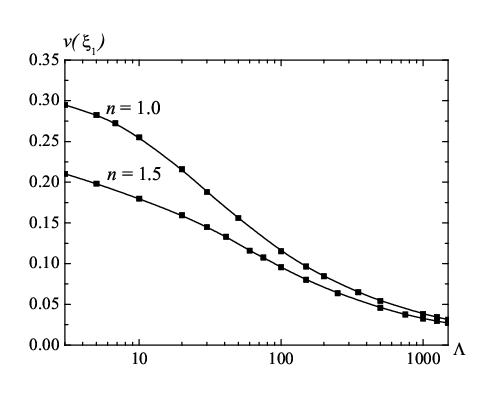
Next, using the data from the tables, in figure 2 we plot , which is proportional to the total mass of the configuration , on the value of the self-coupling parameter at some constant central . In figure 2 we plot as a function of the value of central for different values and . From figure 2 one can see that, while increases, the masses of the configurations decrease both for and . Initially, for small , the masses are very different for and ; asymptotically, for large , they approach comparable values. This is because for large the total mass is defined by the scalar field but not by the contribution from the fluid. The sizes of the configurations are different for the two cases (which has a size characterized by ) and (which has a size characterized by ).
On the other hand if one fixes the size of the star to equal the size of a corresponding relativistic configuration without a scalar field, and changes the central value of so as to get regular solutions, it is necessary to choose appropriate eigenvalues of and . In this case as a function of is given in figure 2. From this figure one sees that as increases the mass of the configuration can either increase (for the case) or decreases (for the case).
It follows from tables 1, 2 and figures 2, 2 that the masses of the configurations, computed for the values of the system parameters used here, are considerably smaller than the masses of the stars without a scalar field. The maximal dimensionless masses of the configuration with the scalar field for and at are and , respectively; without a scalar field the masses of the same configurations are and , respectively. Our attempts to increase the masses of the system by varying were not successful. From figure 2 the implication is that the masses change only slightly with .
Next, in figure 3 the metric functions , and the mass distribution (as a function of the dimensionless radius ) are given. In plotting these functions we used the following procedure:
Inside the Star: The function was plotted using (13); the function was plotted from equation (14), in terms of the dimensionless variables from (16). Explicitly
| (30) |
From the interior solution parts of figure 3 (i.e. the region ) we see the reason for the terminology “chameleon star” for the present solutions – the scalar field mimics the behavior of the fluid in the interior region. Even in the exterior region where the fluid goes to zero the scalar field is asymptotically going to zero.
Outside the star: The solution goes to the Schwarzschild solution
| (31) |
The mass function is defined as
Finally, in figures 5 and 5 we plot the energy density, , from the expression (29). The definition of the mass function given just above takes into account the energy of the fluid and the scalar field from to . Although the fluid vanishes at the scalar field does not vanish. Thus in principle one should include the contribution to the mass function of the scalar field from to . However from the figures 3-5 one can see that and rapidly go to zero as and thus the mass function is given essentially just by the fluid and scalar field energy density between and .
We now turn the the question of connecting the interior region (i.e. where one has both fluid plus scalar field as a source) with the exterior region (i.e. where one has only a rapidly vanishing scalar field). For this purpose, we write down the Einstein equations of (4) and (5), and the scalar field equation of (6), without the fluid source i.e. so that from (9) and (10) we have zero pressure and density. This leads to the following system of equations:
| (32) | |||
| (33) | |||
| (34) |
which, by analogy with the transformations made above, can be rewritten in terms of the dimensionless variables and as follows
| (35) | |||
| (36) | |||
| (37) |
where is given by (30), and is taken from (23). Note that this system of equations (32)-(34) (or (35)-(37)) is essentially the same as those obtained in [14] which considered a real scalar field with quartic self-interaction. The above system contains the parameter as a trace of the influence of the fluid on the external solution. The solution sought beginning from the surface of the star at using, as the boundary conditions, the values of and obtained from the solution of the equations (24)-(26) for the internal part of the configuration. This allows one to determine the value of the integration constant from (13) by requiring to be equal to unity at infinity, providing asymptotical flatness of the space-time. (The values of for the examples shown in figures 3 are given in the caption.) Thus the complete solution for the configuration under consideration is derived by matching of the internal fluid solutions given by equations (24)-(26) with the external solutions obtained from the system (35)-(37).
The system (35)-(37) has obvious asymptotically flat solutions in the form: with taken from (31) that corresponds to the fact that, by choosing the eigenvalues of the parameters and presented in tables 1 and 2, the external scalar field makes negligible contribution to the total mass of the configuration. It allows using the solution for the metric functions in the form of (31) as a good approximation; , where the constant is made equal to zero by the corresponding choice of (see above); . The numerical calculations of the system (35)-(37) confirm this asymptotic behavior.
From figures 3, 5 and 5 we can draw the following conclusions about the metric functions, and the mass distribution :
(1) Asymptotically, as , the space-time becomes flat, i.e. . To get this asymptotic behavior of the metric function , it is necessary to choose a specific value for the central value, (see the caption of figures 3). The asymptotic behavior of follows from equation (30) and the fact that as .
(2) As shown in [28], the relativistic configurations without a scalar field are characterized by a greater concentration of matter toward the center than in the non-relativistic case. By including a scalar field, we obtain even greater concentration of matter toward the center. This can be seen by comparing figures 3 with figures 1 and 2 from the paper [28]. The main reason for the increased concentration of mass is the non-minimal coupling between the scalar field and the fluid with the choice of the coupling function given by (22). The functional form of this coupling gives the required regular solutions, lying in the range , only for the eigenvalues of the parameter (see tables 1, 2). This leads to the fact that near the origin, when , a greater concentration of mass occurs due to the presence of the term in the expression for the energy density (29). At the same time both and give relatively small contributions to the energy density compared to the term coming from the non-minimal scalar-fluid coupling. This fact will become important, below, when we consider the stability of the solutions.
(3) The total energy density presented in figures 5 and 5 strongly depends on the polytropic index . At comparable central values of the scalar field the energy density for the case is several times greater than for the case . In turn, both values of yield a greater energy density at the center of the configurations than in the case of the relativistic stars without a scalar field [28] when the energy density was found to be 1.
(4) Despite the higher concentration of matter at the center of the configurations with the addition of the scalar field, their masses are considerably smaller than the masses of the relativistic stars of the same size but without a scalar field (see table 2). This occurs as a consequences of the fact that the external region of the stars, with only the scalar field as a source, is strongly rarefied due to the rapid vanishing of the scalar field in the region .
IV.2 Non-relativistic case
In this section we consider the non-relativistic limit of the system (24)-(26). The non-relativistic limit corresponds to , and . First, we recall some results about this system in the absence of the scalar field [32]. With no scalar field the system of equations (24)-(26) reduces to the well known Lane-Emden equation
| (38) |
This equation has solutions which describe finite size configurations for different values of the parameter [32]. The non-relativistic limit for the case when there a scalar field is obtained by omitting all terms with in equations (24)-(26) except for the term in the scalar field equation (26). This term must be kept since the product is generally a non-zero quantity even for . Taking all the above into account we rewrite the system (24)-(26) in the following form:
| (39) | |||||
| (40) | |||||
| (41) |
Here, as in the relativistic case the presence of the term is important – it leads to a change in sign of the effective mass term for certain values of . This feature is important for the existence of regular solutions.
Proceeding as in the previous section, we obtain numerical results for the non-relativistic limit which we present in table 3. We chose the parameter to be . Such a small value of requires that be large enough so that the first term on the right hand side of equation (41) is negative, which is the necessary condition to have regular solutions. In the non-relativistic case, as in the relativistic case, we need to find eigenvalues of two parameters and in order to have regular solutions for a given values of the polytropic index, , and the central value of the scalar field, . From table 3 we do indeed find that there are values of large enough to make the first term on the right hand side of (41) negative thus yielding regular solutions.
| , | ||||||
| Non-relativistic star without a scalar field | ||||||
| 3.6538 | 2.7141 | 5.9907 | 0.0000 | |||
| Non-relativistic star with the scalar field | ||||||
| 0.039 | 1040 | 20600 | 3.6538 | 0.4384 | 37.0928 | -0.0009 |
| 0.038 | 1850 | 21800 | 3.6538 | 0.4373 | 37.1840 | -0.0009 |
| 0.036 | 3980 | 24500 | 3.6538 | 0.4354 | 37.3411 | -0.0009 |
| 0.034 | 7010 | 27600 | 3.6538 | 0.4346 | 37.4105 | -0.0009 |
| 0.030 | 17575 | 35500 | 3.6538 | 0.4349 | 37.3895 | -0.0009 |
| 0.028 | 25895 | 39500 | 3.6538 | 0.4462 | 36.4388 | -0.0009 |
| 0.027 | 31270 | 41700 | 3.6538 | 0.4556 | 35.6855 | -0.0009 |
| , | ||||||
| Non-relativistic star without a scalar field | ||||||
| 3.1416 | 3.1416 | 3.2899 | 0.0000 | |||
| Non-relativistic star with the scalar field | ||||||
| 0.039 | 190 | 10700 | 3.1416 | 0.6568 | 15.7364 | -0.0008 |
| 0.038 | 595 | 11000 | 3.1416 | 0.6687 | 15.4556 | -0.0008 |
| 0.036 | 1645 | 12000 | 3.1416 | 0.6761 | 15.2872 | -0.0008 |
| 0.034 | 3070 | 13100 | 3.1416 | 0.6868 | 15.0493 | -0.0008 |
| 0.030 | 7645 | 15700 | 3.1416 | 0.7166 | 14.4227 | -0.0008 |
| 0.025 | 20685 | 21000 | 3.1416 | 0.7457 | 13.8609 | -0.0008 |
Using the data from table 3, the dependence of the on the central value of the scalar field is given in figure 7. Figure 7 uses the date from table 3 to plot the ratio of the energy density to the central density, as a function of the dimensionless, normalized radius. Also from table 3 one can see that we have fixed the radius of a star to be equal to the size of a non-relativistic star without a scalar field. From the figure we can draw the following observations:
(1) The masses of the stars with a scalar field are considerably smaller than the masses of the stars without a scalar field. In the case the masses are 4-5 times smaller, and in the case about 6 times smaller.
(2) The mass is a fairly slowly varying function of , especially when .
(3) There is a greater concentration of the mass density towards the center of the stellar configurations. This can be seen explicitly by comparing with the distribution of the mass density for a star without a scalar field which is also presented in figure 7.
All these results are very similar to those of the relativistic case.


IV.3 Stability of the solutions
In this section we discuss the issue of the stability of the regular solutions obtained above. There are two basic approaches to studying the stability: (i) The energy approach to the theory of equilibrium for a star [32]; (ii) A more rigorous dynamical stability approach based on studying the stability of linear and nonlinear time-dependent perturbations. In this paper we will use the first approach. Proceeding along the lines of reference [28], we define the total energy of the system, including the internal and gravitational energies, as
| (42) |
where is defined by (2) and corresponds to the total energy density of the system (recall that ). Next, we consider a system consisting of a gas of particles having a rest-mass density . Its relativistic energy density is the sum of the rest energy plus the density of internal energy. For the special case of an adiabatic process which assumes the absence of heat flow terms in the energy-momentum tensor (2), it is possible to obtain a relation between the gas density and the total mass density or alternatively between and , .
To do this we use the first law of thermodynamics which, in our case, takes the form
| (43) |
where is the total pressure, and is the specific volume (this symbol should not be confused with the potential energy used earlier). Since , equation (43) gives the following relation
| (44) |
In general, when and are functions of , this equation cannot be integrated. However, for our configuration, the numerical calculations performed in the previous sections show that the main part of the energy is provided by the term containing the non-minimal coupling but not by and . This allows us to neglect the terms containing the scalar field kinetic energy and potential as compared with and in the and components of the energy-momentum tensor (2), respectively. In this approximation we have the following expressions for the total mass density and the pressure:
Substituting these expressions into (44) and taking into account that and , we have from (44):
This equation differs from the case without a scalar field by the presence of the second term on the right-hand side containing the coupling function . In the absence of the non-minimal coupling, i.e. when , this term vanishes. Integrating, we find
| (45) |
where is the value of the gas density at the center of the configuration. This constant may be evaluated as follows [28]: near the boundary of the configuration, where , equation (45) becomes approximately
where is the point starting from which the approximation becomes valid. This equation can be rewritten in differential form as
| (46) |
Since is a function of , the term on the right-hand side can be evaluated as follows
Taking this expression into account, equation (46) takes the form
Near the boundary the internal energy density is small compared to the rest-mass energy density, so that . Comparing the above equation with the expression , we obtain
and equation (45) becomes
| (47) |
Using expression (47), the corresponding proper energy of the gas may be defined as the integral of with respect to proper volume for the metric (3) as follows
| (48) |
The quantity is proportional to the total number of particles in the configuration, , where is Avogadro’s number. Using the dimensionless variables (16) and expressions (30), (47), we obtain the proper energy of the gas (48) in units of the total energy in the following form
| (49) |
This expression differs from the corresponding expression in [28] through the presence of an extra factor under the integral which comes from the non-minimal coupling in the system. Stability of the configuration can tested via the sign of the expression [28, 32]
| (50) |
The necessary (but not a sufficient) condition for stability of the system that i.e. that the total system energy is less that the energy of the non-gravitationally interacting gas, , making the energetically preferred state. The condition in (50) amounts to requiring that the Binding Energy defined in this equation be positive. In the paper [34], the question of stability of adiabatic polytropic configurations was considered. It was shown that such configurations may have both positive and negative binding energies depending on the value of the polytropic index , and the parameter (configurations with and were considered).
When a non-minimally coupled scalar field is included, we considered a very narrow range of these parameters, and , and also only one choice of the coupling function given by the form (22). In this case the numerical calculations indicate that , i.e. we have the negative binding energy, and correspondingly the configurations under consideration are unstable. The same values of and without a scalar field give configurations with the positive binding energy [34]. Obviously, the difference between the present results and those of [34] is connected with the presence of the extra factor under the integral in the expression (49) whose value, as numerical calculations indicate, is much less than unity for the parameters , used in the paper, and for the coupling function of the form (22).
The behavior of in (49) can be approximately estimated as follows: Since we are looking only for solutions with , the value of may be approximated as giving a finite contribution to the value of integral in the form of some constant factor , i.e. . Then one can see that
When the coupling function is taken in the form (22), we have the finite value of , and since then as well, thereby suppressing the value of in (49). In the non-relativistic case, where , we have and the situation with the instability is the same.
Possible ways of resolving this problem are:
(i) Consider configurations for which , and the function varies slowly in the range to provide a large value of the above . In this case, one can expect that the configuration will have a “tail” of a scalar field outside the fluid at (a similar thing happens for configurations considered in [5]). In this case, it will be necessary to perform a stability analysis of both internal solutions (where the fluid and the scalar field are involved) and external solutions (where only the scalar field is involved).
(ii) Since the solutions and their stability are sensitive to the nature of the scalar field-fluid coupling, which in this paper was take to have the form given in (22), one could look for stable solutions by examining different forms of this coupling; for example one could try a non-polynomial coupling of the form . These stability studies will be the focus of future work.
V Non-relativistic case: an analytical solution for a massless scalar field
The numerical results obtained in the previous sections demonstrate the possibility of obtaining the regular solutions both in relativistic and non-relativistic cases when the coupling function is chosen in the form of (22). This choice is not the only one possible. It will be shown latter in this section that, by choosing the special form of the function , it is possible to find an analytical solution in a particular non-relativistic case when the polytropic index , and the scalar field is taken to be massless. This case corresponds to an incompressible fluid with a constant mass density, , and a spatial varying pressure, .
To begin we rewrite the system of equations (24)-(26) for the massless case and in the non-relativistic limit () in the form
| (51) | |||||
| (52) | |||||
| (53) |
We have kept the -containing-term on the right-hand side of equation (53) since it is does not necessarily small for arbitrary . Differentiating the first equation of the system, and substituting the second and the third equations into this expression, gives
| (54) |
The last term of this equation contains the factor . For , equation (54) reduces to the Lane-Emden equation (38) which has an analytical solution for the case of an incompressible fluid with a constant mass density – see [32], equation (10.3.14). This solution is
| (55) |
Equation (54) can also be integrated analytically by choosing the function to have the following power-law form
| (56) |
where , and are arbitrary parameters. Using this function and taking the parameter to be of order 1 so that the product , we have from (54):
When , this equation can be integrated giving the following regular solution
| (57) |
Here is an integration constant. A second integration constant was set equal to zero to make the solution regular at . We take so that in the absence of the scalar field (i.e. when and ) equation (57) will reduce to equation (55). This solution is regular everywhere, including the point , when . The degenerate case corresponds to the classical solution (55) which can be obtained from (57) by setting and . This choice that corresponds to turning equation (54) into the Lane-Emden equation (38).
We now analyze the behavior of the solution as . To begin we calculate the first and second derivatives of :
For a spherically symmetric solution with maximal mass density as , two conditions must be satisfied: (1) the first derivative must be equal to zero; (2) the second derivative must be negative. The former condition gives . Given this the behavior of the second derivative is:
| if : | |
| if : | for any . |
One can see that for the second condition is satisfied only if .
On the other hand, the regularity of the solution assumes the presence of a point on the axis, , where . For the classical solution (55), this point is . In the case of configurations with a scalar field, the location of the point will depend on the factors in front of the term in (57), i.e. it will be determined by the values of and the denominator . In the range only negative are allowed if one wants as , which is one of conditions that the solution (57) be regular. In the range the regularity of the solution is guaranteed if , since otherwise the solution grow as a power law of .
The above analysis shows that the inclusion of a scalar field decreases the size of configurations, as compared to the classical case (55), for all acceptable values of the parameter . In this sense the behavior of the solutions with a massless scalar field and the coupling function in the form of (56) differs from the behavior of the solutions obtained in section IV.2 when the function was chosen to have the form (22). In the latter case, the size of the configurations for given values of and depends considerably on the parameters , , and , and it can be larger or smaller than the size of a configuration without a scalar field.
Substituting the expression for from (57) into the scalar field equation (53) with , we find the following analytical solution for the scalar field in the interior of the configuration
| (58) |
One can see from this expression that the behavior of the scalar field is defined in large measure by the factor in front of the square brackets. Since in the non-relativistic limit , this factor will differ appreciably from zero only for large . For not large one can expect that the field will be practically constant and equal to the central value up to the boundary of the fluid at where . The general solution for for all is obtained by matching of the internal solution (58) with an external solution of equation (53) where the right-hand side is equal to zero. The exterior equation has a solution of the form
where are integration constants which are determined by matching of the external solution with the interior solution solution at the boundary of the fluid at . One can see from this expression that the corresponding mass density, which is proportional to , tends asymptotically to zero.
VI Conclusion
In this article we studied gravitating, spherically symmetric, star-like, configurations with a matter source consisting of a normal (i.e. non-ghost, non-phantom) scalar field plus a perfect isotropic fluid. The motivation for studying such a model is that scalar fields have found broad use in various cosmological models as well as astrophysical models. It is natural to postulate that, if scalar fields do really play a role in the Universe that these scalar fields might play a role in the structure of compact objects such as Main Sequence stars or neutron stars. Proceeding from this assumption, we studied a model of a star-like configuration supported by a scalar field non-minimally coupled to ordinary matter in the form of a perfect fluid. As an example, we considered the case when the scalar field had a quadratic mass term and a quartic self-interaction giving a scalar field potential of the form (23). The coupling between the scalar field and the perfect fluid, , was taken to have the form (22). For this model we studied solutions both in the relativistic and non-relativistic limit. Our investigation showed that the existence of regular solutions is possible exactly because of the presence of the non-minimal coupling between the scalar field and fluid. In the absence of such coupling, the potential (23) gives only singular solutions [14]. From the mathematical point of view, the existence of regular solutions in our model is possible because of the appearance in scalar field equation (26) of an effective mass term whose sign depends both on the behavior of the fluid density and the values of the parameters and . It was shown that when , there were regular solutions with finite masses and sizes. In some sense the solutions presented above are a cross between the interacting scalar field solutions of [33] and the interacting real scalar field solutions of [14]. In the interior region, , we have a real scalar field and a fluid which interacts with the scalar field. Due to the chameleon-like behavior of the scalar field with respect to the fluid (from figure 3 one can see that in the interior region the field mimics the fluid) one might think of the two degrees of freedom associated with the scalar field and the fluid as being equivalent to the two degrees of freedom of a complex scalar field. While there is certainly some validity in this analogy (both the present solutions and those in [33] are non-singular) one must avoid pushing the analogy too far since the fluid vanishes exactly at some point (i.e. at ) while the complex scalar field of [33] and the real scalar of the present solution only go to zero asymptotically. Thus after reaching the point our solutions become those of [14].
Our results are interesting since they show that by adding such a fluid one can find regular solutions, thus evading some gravitational version of Derrick’s theorem [23, 24] which prohibits regular solutions for the system of gravity plus a normal scalar field if the potential . Thus the addition of the fluid was crucial to the existence of these solutions. The original, non-gravitational version of Derrick’s theorem [21, 22] assumes not merely the regularity of solutions, but also their stability. In this paper we have performed a preliminary stability analysis based on energy considerations. In this case we compared the total energy of the system (including the internal and gravitational energies) and the rest energy of the gas particles. For the values of the polytropic index and the parameter , and the specific coupling function in the form of (22), this energy approach showed that the solutions studied in this paper are unstable. This was because the binding energy of the system, which was equal to the difference of the rest energy and the total energy, was negative. But, as it was shown in [34], even a positive binding energy does not guarantee stability of a system allowing its transition to an energetically more advantageous state with the same polytropic index , but having another parameter . Obviously, such process is accompanied by an ejection of the excess of energy. In our case, the possibility is not excluded that there exist regular solutions with positive binding energy, for other values of and and other parameters of the scalar field . There is an additional possibility for finding stable solutions which was described at the end of section IV.3 – since the solutions and their stability are sensitive to the form of the scalar field-fluid coupling (which in the present work had the form (22)) one could look for stable solutions by changing the form of the scalar field-fluid coupling. For example, one could try non-polynomial couplings of the form . Finally, the energy approach to stability which was used in this paper, can and should be supplemented by a study of dynamical stability along the lines of the linear stability analysis performed in [14, 18, 20] or by using the catastrophe theory method suggested in [35]. In future work we plan to perform a stability analysis of the chameleon star solutions investigated here using both these approaches.
The spherically symmetric solution that we found for the system considered in this paper were called chameleon stars in analogy with chameleon cosmological models [10] because the characteristics of the scalar field (e.g. its mass) strongly depend the other fields and fluids in its environment. We characterized the behavior of these chameleon star configurations for both relativistic and non-relativistic cases. For the relativistic chameleon stars we found that in general the mass-energy density tended to be more concentrated toward the center of the star at . Despite this greater concentration of mass near the center of the chameleon star the total mass of the chameleon star was lower than the corresponding relativistic stars without a scalar field. This was the result of the outer regions of the chameleon star being much less dense than a corresponding non-chameleon, relativistic star. Similar comments apply to the non-relativistic chameleon stars. For the non-relativistic case we were able to find an analytical solution for the case when the scalar field was massless. This analytical solution had similar behavior to the numerically obtained solutions from section IV.2.
We briefly give some speculations about possible physical applications of the present solutions. Scalar fields are thought to play a role in cosmological dynamics (dark energy) and in dynamics at the galactic scale (dark matter). The present proposal is that a scalar field could play some role in astrophysics at the stellar scale in the formation of the chameleon star configurations discussed here. The fluid in our model would be provided by the star. For example one could consider neutron stars which contain a significant amount of the scalar field. From the discussion above our chameleon stars – both relativistic and non-relativistic – would be less massive for a given radius despite having a higher concentration of mass near the center. Thus one might look for neutron stars which have a larger radius for a given mass than would be expected for a normal neutron star. In this sense chameleon stars would have the opposite behavior from hypothetical quark stars which have a larger mass for a given radius. Another possibility is that some living stars (i.e. stars which are still fusing elements and are on the Main Sequence) might have trapped some significant amount of scalar field in their interior. Such living, chameleon stars would tend to have a larger density near their center thus increasing the rate at which they fused elements. The consequence of this is that such stars would be hotter and live a shorter than expected life span for their mass. Again a given chameleon star would have less overall mass than a non-chameleon star but would be nevertheless have a higher, interior temperature. The physical applications of the chameleon star model suggested above would of course require the existence of stable solutions. A search for such stable solutions is a goal of future studies.
Acknowledgements
V.D. and V.F. are grateful to the Research Group Linkage Programme of the Alexander von Humboldt Foundation for the support of this research.
Appendix A Derivation of the energy-momentum tensor
In the case of the isentropic quasipotential flow, the Lagrangian of the continuous medium has the form [29, 30]
| (A.1) |
where is the heat function, and is the energy density. Introducing the quasipotential
where is the velocity of light and is the action for the matter, we have
from which it follows
The Lagrangian (A.1) now takes the form
| (A.2) |
The total action (including gravity plus all matter sources) in curvilinear coordinates is [36]
| (A.3) |
where the Lagrange density, , above is that given in equation (1). By varying the action (A.3) with respect to the metric, , one can obtain the Einstein equations and the energy-momentum tensor. In this way the energy-momentum tensor is given by the expression
| (A.4) |
where the Lagrangian, , contains only the matter components of the Lagrangian (1) namely
Since does not depend on , the last term in (A.4) equals zero. Then we have
| (A.5) |
Taking into account that and also using the expressions (A.1) and (A.2), we find
and
Substituting these expressions into (A.5), we finally have:
| (A.6) |
References
- [1] A. Linde, Particle Physics and Inflationary Cosmology, Harwood, Chur (1990); hep-th/0503203.
- [2] E. J. Copeland, M. Sami and S. Tsujikawa, Int. J. Mod. Phys. D 15, 1753 (2006) [arXiv:hep-th/0603057].
- [3] G. Bertone, D. Hooper, J. Silk, Phys. Rept. 405, 279-390 (2005). [hep-ph/0404175].
- [4] F. E. Schunck, E. W. Mielke, Class. Quant. Grav. 20, R301-R356 (2003). [arXiv:0801.0307 [astro-ph]].
- [5] V. Dzhunushaliev, V. Folomeev, B. Kleihaus and J. Kunz, JCAP 1104, 031 (2011) [arXiv:1102.4454 [astro-ph.GA]].
- [6] T. D. Lee and Y. Pang, Phys. Rev. D 35, 3678 (1987).
- [7] A. B. Henriques, A. R. Liddle and R. G. Moorhouse, Phys. Lett. B 233, 99 (1989).
- [8] A. B. Henriques, A. R. Liddle and R. G. Moorhouse, Nucl. Phys. B 337, 737 (1990).
- [9] P. Jetzer, Phys. Lett. B 243, 36 (1990).
- [10] H. Farajollahi and A. Salehi, Int. J. Mod. Phys. D 19, 621 (2010) [arXiv:1004.3508 [gr-qc]].
- [11] F. Cannata and A. Y. Kamenshchik, Int. J. Mod. Phys. D 20, 121 (2011) [arXiv:1005.1878 [gr-qc]].
- [12] J. Khoury and A. Weltman, Phys. Rev. D 69, 044026 (2004) [arXiv:astro-ph/0309411].
- [13] M. Wyman, Phys. Rev. D 24, 839 (1981).
- [14] P. Jetzer and D. Scialom, Phys. Lett. A 169, 12 (1992).
- [15] T. Kodama,Phys. Rev. D 18, 3529 (1978).
- [16] T. Kodama, L.C.S. de Oliveira, and F.C. Santos, Phys. Rev. D 19, 3576 (1979).
- [17] V. Dzhunushaliev, V. Folomeev, R. Myrzakulov and D. Singleton, JHEP 0807, 094 (2008) [arXiv:0805.3211 [gr-qc]].
- [18] M.A. Clayton, L. Demopoulos, and J. Légaré, Phys. Lett. A 248, 131 (1998).
- [19] T. Torii, K. Maeda and M. Narita, Phys. Rev. D 59, 104002 (1999).
- [20] V. Dzhunushaliev, V. Folomeev, R. Myrzakulov and D. Singleton, Phys. Rev. D 82, 045032 (2010) [arXiv:1006.1527 [gr-qc]].
- [21] G.H. Derrick, J. Math Phys. 5 1252 (1964).
- [22] R. Rajaraman, An Introduction to Solitons and Instantons in Quantum Field Theory (North-Holland Publishing Company, Amsterdam, New York, Oxford, 1982).
- [23] K. A. Bronnikov, S. B. Fadeev, A. V. Michtchenko, Gen. Rel. Grav. 35, 505-525 (2003). [gr-qc/0212065].
- [24] K. A. Bronnikov and J. C. Fabris, Phys. Rev. Lett. 96, 251101 (2006) [arXiv:gr-qc/0511109].
- [25] G. ’tHooft, Nucl. Phys. B 79, 276 (1974).
- [26] A.M. Polyakov, JETP Lett. 20, 194 (1974).
- [27] S. Chandrasekhar, An Introduction to the Study of Stellar Structure (Chicago: University of Chicago Press; New York: Dover Publications, 1957).
- [28] R. Tooper, Astrophys. J. 140, 434 (1964).
- [29] K.P. Stanukovich, Soviet Physics Doklady 9, 63 (1964).
- [30] K.P. Stanukovich, Unsteady flows of continuous medium, Nauka, Moscow, 1971. (In Russian.)
- [31] O. Bertolami, F. S. N. Lobo and J. Paramos, Phys. Rev. D 78, 064036 (2008) [arXiv:0806.4434 [gr-qc]].
- [32] Ya. B. Zel’dovich, I. D. Novikov, Stars and relativity (Mineola, New York: Dover Publications, 1996).
- [33] M. Colpi, S. L. Shapiro, I.Wasserman, Phys. Rev. Lett. 57, 2485 (1986).
- [34] R. Tooper, Astrophys. J. 142, 1541 (1965).
- [35] F. V. Kusmartsev, E. W. Mielke, and F. E. Schunck, Phys.Rev. D 43, 3895 (1991)
- [36] L. Landau, E. Lifshitz, The classical theory of fields (Pergamon, Oxford, 1987).