Transverse Momentum Dependent Parton Density Functions and a Self-Similarity based Model of Proton Structure Function $F_{2}(x,Q^{2})$ at Large and Small $x$

One of the most intriguing problems in QCD is the growth of the cross-sections for hadronic interactions with energy. Conventionally deep inelastic lepton-hadron scattering is described in terms of scale-dependent parton distributions $xg(x,k_{t}^{2})$ and $xq(x,k_{t}^{2})$. These distributions correspond to the density of partons in the proton with longitudinal momentum fraction x and parton transverse momentum $k_{t}^{2}$ [17].

The self-similarity based Model of the nucleon structure function proposed in Ref. [7, 8] has been designed to be valid at small Bjorken-x. The formalism described in these references is based on the imposition of self-similarity constraints to the dimensionless TMD quark density $f_{i}(x,k_{t}^{2})$ and relate it to the integrated density. In other words, using magnification factors $\displaystyle\frac{1}{x}$ and $\displaystyle\left(1+\frac{k_{t}^{2}}{Q_{0}^{2}}\right)$, an unintegrated quark density (TMD) is given as:

$$\log f_{i}(x,k_{t}^{2})=D_{1}\log\frac{1}{x}\log\left(1+\frac{k_{t}^{2}}{Q_{0}^{2}}\right)+D_{2}\log\frac{1}{x}+D_{3}\log\left(1+\frac{k_{t}^{2}}{Q_{0}^{2}}\right)+D_{0}^{i}$$

(5)

where i denotes a quark flavor. Here, $D_{2}$ and $D_{3}$ are the fractal parameters; $D_{1}$ is the dimensional correlation relating the two magnification factors; while $D_{0}^{i}$ is the normalization constant. Conventional integrated quark densities [PDF] $q_{i}(x,Q^{2})$ are defined as sum over all contributions with quark virtualities smaller than that of the photon probe $Q^{2}$. Thus $f_{i}(x,k_{t}^{2})$ has to be integrated over $k_{t}^{2}$ (Eq (2)) to obtain $q_{i}(x,Q^{2})$.

The following analytical parameterization of a quark density is obtained by using Eq (2).

$$q_{i}(x,Q^{2})=\frac{e^{D_{0}^{i}}Q_{0}^{2}x^{-D_{2}}}{1+D_{3}+D_{1}\log\frac{1}{x}}\left(x^{-D_{1}\log\left(1+\frac{Q^{2}}{Q_{0}^{2}}\right)}\left(1+\frac{Q^{2}}{Q_{0}^{2}}\right)^{D_{3}+1}-1\right)$$

(6)

Now using Eq (6) in Eq (1), the expression for proton structure function is obtained as:

$$F_{2}(x,Q^{2})=\frac{e^{D_{0}}Q_{0}^{2}x^{-D_{2}+1}}{1+D_{3}+D_{1}\log\frac{1}{x}}\left(x^{-D_{1}\log\left(1+\frac{Q^{2}}{Q_{0}^{2}}\right)}\left(1+\frac{Q^{2}}{Q_{0}^{2}}\right)^{D_{3}+1}-1\right)$$

(7)

where $D_{0}=\Sigma_{i}D_{0}^{i}$ .

As we have seen above, Lastovicka’s Model starts with self-similar TMDPDFs. Imposing large x limit, i.e. at $x\rightarrow 1$, Eq (7) becomes:

$$F_{2}(1,Q^{2})=\frac{e^{D_{0}}Q_{0}^{2}}{1+D_{3}}\left(\left(1+\frac{Q^{2}}{Q_{0}^{2}}\right)^{D_{3}+1}-1\right)$$

(8)

Let

$$\tilde{F}_{2}(1,Q^{2})=\frac{F_{2}(1,Q^{2})}{e^{D_{0}}Q_{0}^{2}}=\frac{1}{1+D_{3}}\left(\left(1+\frac{Q^{2}}{Q_{0}^{2}}\right)^{D_{3}+1}-1\right)$$

(9)

If $F_{2}(1,Q^{2})=0$, then we get $D_{3}=-1$ and subsequently $\tilde{F}_{2}(x,Q^{2})$ becomes indeterminate (using Eq (9)). It implies that the Model does not have correct $x\rightarrow 1$ behavior. This calls for generalization of PDFs to add a new term in TMDPDFs. A plausible way to incorporate correct $x\rightarrow 1$ behavior for TMDPDF is to introduce an additional term $h(x,k_{t}^{2})$ which does not have fractal basis.

Now, starting with the TMDPDF, we have:

	$\displaystyle logf_{i}(x,k_{t}^{2})$	$\displaystyle=$	$\displaystyle D_{1}\log\frac{1}{x}\log\left(1+\frac{k_{t}^{2}}{Q_{0}^{2}}\right)+D_{2}\log\frac{1}{x}+D_{3}\log\left(1+\frac{k_{t}^{2}}{Q_{0}^{2}}\right)+$		(10)
			$\displaystyle{}D_{0}^{i}+\log h(x,k_{t}^{2})$

i.e.

$$f_{i}(x,k_{t}^{2})=\left(\frac{1}{x}\right)^{D_{1}\log\left(1+\frac{k_{t}^{2}}{Q_{0}^{2}}\right)}\left(\frac{1}{x}\right)^{D_{2}}\left(1+\frac{k_{t}^{2}}{Q_{0}^{2}}\right)^{D_{3}}e^{D_{0}}h(x,k_{t}^{2})$$

(11)

Thus the integrated quark density is given as:

$$q_{i}(x,Q^{2})=\int\limits_{0}^{Q^{2}}\,dk_{t}^{2}\left(\frac{1}{x}\right)^{D_{1}\log\left(1+\frac{k_{t}^{2}}{Q_{0}^{2}}\right)}\left(\frac{1}{x}\right)^{D_{2}}\left(1+\frac{k_{t}^{2}}{Q_{0}^{2}}\right)^{D_{3}}e^{D_{0}^{i}}h(x,k_{t}^{2})$$

(12)

In the simplest case, consider $h(x,k_{t}^{2})$ to be only x-dependent, i.e. $h(x,k_{t}^{2})\approx h(x)$.
Then, the improved model is

$$F_{2}^{I}(x,Q^{2})=F_{2}(x,Q^{2}).h(x);\qquad\qquad where\quad 0\leq x\leq 1$$

(13)

where $F_{2}(x,Q^{2})$ is the original Lastovicka’s model (Eq (7)).

Neglecting $k_{t}^{2}$ dependence of $h(x,k_{t}^{2})$, the most economical way of having correct large x behavior is $h(x,k_{t}^{2})\approx h(x)\sim(1-x)^{\alpha},\mathrm{for}\;\alpha>0$, but in general the integration is to be carried out with its explicit $k_{t}^{2}$ dependence in Eq (12). Thus large x effect should be introduced as an additional component of TMDPDF to make the PDF compatible with the theoretical expectation, i.e. $F_{2}(x,Q^{2})\rightarrow 0$ as $x\rightarrow 1$ [22, 23, 24].

In general, TMDPDF depends on two hard scales, parton transverse momentum $k_{t}^{2}$ and the scale $Q^{2}$ of the probe [20, 38, 39]. In Fractal Inspired Model (Lastovicka’s), it will therefore have three magnification factors, viz. $\displaystyle\frac{1}{x}$, $\displaystyle\left(1+\frac{k_{t}^{2}}{k_{0}^{2}}\right)$ and $\displaystyle\left(1+\frac{Q^{2}}{Q_{0}^{2}}\right)$; and four correlation terms. The generalization of TMDs of this Model is therefore given as:

	$\displaystyle logf_{i}(x,k_{t}^{2},Q^{2})=$				(14)
			$\displaystyle D_{1}\log\frac{1}{x}\log\left(1+\frac{k_{t}^{2}}{k_{0}^{2}}\right)+D_{2}\log\frac{1}{x}+D_{3}\log\left(1+\frac{k_{t}^{2}}{k_{0}^{2}}\right)+$
			$\displaystyle D_{4}\log\left(1+\frac{Q^{2}}{Q_{0}^{2}}\right)+D_{5}\log\frac{1}{x}\log\left(1+\frac{Q^{2}}{Q_{0}^{2}}\right)+$
			$\displaystyle D_{6}\left(1+\frac{k_{t}^{2}}{k_{0}^{2}}\right)\left(1+\frac{Q^{2}}{Q_{0}^{2}}\right)+D_{7}\log\frac{1}{x}\log\left(1+\frac{k_{t}^{2}}{k_{0}^{2}}\right)\left(1+\frac{Q^{2}}{Q_{0}^{2}}\right)+$
			$\displaystyle D_{8}\log h\left(x,k_{t}^{2},Q^{2}\right)+D_{0}^{i}$

where $h(x,k_{t}^{2},Q^{2})$accounts for large x behavior.

In the above Eq (14), there are altogether eight parameters, viz.$D_{2}$, $D_{3}$, $D_{4}$ (Fractal dimensions);$D_{1}$, $D_{5}$, $D_{6}$, $D_{7}$ (Correlation parameters) and $D_{0}^{i}$ (Normalization constant); as well as one unknown function $h(x,k_{t}^{2},Q^{2})$.

While $D_{1}$, $D_{5}$, $D_{6}$, $D_{7}$ are the correlation parameters correlating the different magnification factors, $h(x,k_{t}^{2},Q^{2})$ is the additional function that cannot be constrained by the notion of fractal geometry.
Now following the same steps as above, Eq (14) can be rewritten in the following way:

	$\displaystyle f_{i}(x,k_{t}^{2},Q^{2})$	$\displaystyle=$	$\displaystyle e^{D_{0}^{i}}.h(x,k_{t}^{2},Q^{2})\left(\frac{1}{x}\right)^{D_{2}}\left(1+\frac{k_{t}^{2}}{k_{0}^{2}}\right)^{D_{3}}\left(1+\frac{Q^{2}}{Q_{0}^{2}}\right)^{D_{4}}.$		(15)
			$\displaystyle{}\left(\frac{1}{x}\right)^{D_{1}\log\left(1+\frac{k_{t}^{2}}{k_{0}^{2}}\right)}\left(\frac{1}{x}\right)^{D_{5}\log\left(1+\frac{Q^{2}}{Q_{0}^{2}}\right)}\left(1+\frac{k_{t}^{2}}{k_{0}^{2}}\right)^{D_{6}\log\left(1+\frac{Q^{2}}{Q_{0}^{2}}\right)}.$
			$\displaystyle{}\left(\frac{1}{x}\right)^{D_{7}\log\left(1+\frac{k_{t}^{2}}{k_{0}^{2}}\right)\log\left(1+\frac{Q^{2}}{Q_{0}^{2}}\right)}$

The integrated quark density is then given as:

$$q_{i}(x,Q^{2})=e^{D_{0}^{i}}\left(\frac{1}{x}\right)^{D_{2}+D_{5}\log\left(1+\frac{Q^{2}}{Q_{0}{2}}\right)}\left(1+\frac{Q^{2}}{Q_{0}^{2}}\right)^{D_{4}}I(x,Q^{2})$$

(16)

where

	$\displaystyle I(x,Q^{2})$	$\displaystyle=$	$\displaystyle\int\limits_{0}^{Q^{2}}\,dk_{t}^{2}\;h(x,k_{t}^{2},Q^{2})\left(\frac{1}{x}\right)^{D_{1}\log\left(1+\frac{k_{t}^{2}}{k_{0}^{2}}\right)+D_{7}\log\left(1+\frac{k_{t}^{2}}{k_{0}^{2}}\right)\log\left(1+\frac{Q^{2}}{Q_{0}^{2}}\right)}.$		(17)
			$\displaystyle{}\left(1+\frac{k_{t}^{2}}{k_{0}^{2}}\right)^{D_{3}+D_{6}\log\left(1+\frac{Q^{2}}{Q_{0}^{2}}\right)}$

Eq (16) is the most general form of PDF which contains two cut-off parameters: $k_{0}^{2}$ and $Q_{0}^{2}$ .

In a special case, imposing the limit $D_{4}$, $D_{5}$, $D_{6}$, $D_{7}=0$ and $D_{8}=0$ (i.e. $h(x,k_{t}^{2},Q^{2})=1$ [see Eq (14)]), the above integral of Eq (17) becomes:

$$I(x,Q^{2})=\int\limits_{0}^{Q^{2}}\,dk_{t}^{2}\left(\frac{1}{x}\right)^{D_{1}\log\left(1+\frac{k_{t}^{2}}{k_{0}^{2}}\right)}\left(1+\frac{k_{t}^{2}}{k_{0}^{2}}\right)^{D_{3}}$$

(18)

which is the original Lastovicka’s Integral to obtain Eq (6). Now let us proceed to evaluate the integral of Eq (17), in more general case, with the following observation:
The exponent of $\displaystyle\frac{1}{x}$ in Eq (17) can be re-expressed as
$\log\left(1+\frac{k_{t}^{2}}{k_{0}^{2}}\right)\tilde{D}_{1}$ with $\tilde{D}_{1}=\left\{D_{1}+D_{7}\log\left(1+\frac{Q^{2}}{Q_{0}^{2}}\right)\right\}$ .

Similarly, the exponent of $\displaystyle\left(1+\frac{k_{t}^{2}}{k_{0}^{2}}\right)$ in Eq (17) is $\tilde{D}_{3}=D_{3}+D_{6}\log\left(1+\frac{Q^{2}}{Q_{0}^{2}}\right)$.

Without explicit form of $h(x,k_{t}^{2},Q^{2})$, Eq (17) cannot be evaluated analytically.

In the limit $h(x,k_{t}^{2},Q^{2})=1$, Eq (17) then becomes:

$$I(x,Q^{2})=\int\limits_{0}^{Q^{2}}\,dk_{t}^{2}\;\left(\frac{1}{x}\right)^{\tilde{D}_{1}\log\left(1+\frac{k_{t}^{2}}{k_{0}^{2}}\right)}\left(1+\frac{k_{t}^{2}}{k_{0}^{2}}\right)^{\tilde{D}_{3}}$$

(19)

which is again similar to Eq (18), i.e. Lastovicka’s Integral, except that in this case $D_{1}$ is replaced by $\tilde{D}_{1}$ and $D_{3}$ by $\tilde{D}_{3}$ . Eq (19) implies

$$I(x,Q^{2})=\frac{Q_{0}^{2}}{1+\tilde{D}_{3}+\tilde{D}_{1}\log\frac{1}{x}}\left\{x^{-\tilde{D}_{1}\log\left(1+\frac{Q^{2}}{k_{0}^{2}}\right)}\left(1+\frac{Q^{2}}{k_{0}^{2}}\right)^{\tilde{D}_{3}+1}-1\right\}$$

(20)

Now substituting this integral from Eq (20) in Eq (16), we obtain:

	$\displaystyle q_{i}(x,Q^{2})$	$\displaystyle=$	$\displaystyle\frac{e^{D_{0}^{i}}\;Q_{0}^{2}\;\left(\frac{1}{x}\right)^{D_{2}+D_{5}\log\left(+\frac{Q^{2}}{k_{0}^{2}}\right)}}{1+\tilde{D}_{3}+\tilde{D}_{1}\log\frac{1}{x}}\left(1+\frac{Q^{2}}{k_{0}^{2}}\right)^{D_{4}}.$		(21)
			$\displaystyle{}\left\{x^{-\tilde{D}_{1}\log\left(1+\frac{Q^{2}}{k_{0}^{2}}\right)}\left(1+\frac{Q^{2}}{k_{0}^{2}}\right)^{\tilde{D}_{3}+1}-1\right\}$

The expression for the proton structure function $F_{2}^{I}(x,Q^{2})$ can thus be obtained using Eq (21) in Eq (1):

	$\displaystyle F_{2}^{I}(x,Q^{2})$	$\displaystyle=$	$\displaystyle\frac{e^{D_{0}}\;Q_{0}^{2}\;\left(\frac{1}{x}\right)^{D_{2}+D_{5}\log\left(+\frac{Q^{2}}{k_{0}^{2}}\right)-1}}{1+\tilde{D}_{3}+\tilde{D}_{1}\log\frac{1}{x}}\left(1+\frac{Q^{2}}{k_{0}^{2}}\right)^{D_{4}}.$		(22)
			$\displaystyle\left\{x^{-\tilde{D}_{1}\log\left(1+\frac{Q^{2}}{k_{0}^{2}}\right)}\left(1+\frac{Q^{2}}{k_{0}^{2}}\right)^{\tilde{D}_{3}+1}-1\right\}$

where $\tilde{D}_{1}$ and $\tilde{D}_{3}$ are independent of $k_{t}^{2}$ .

As in Eq (7), imposing boundary condition (Eq (4)) at $x\rightarrow 1$, Eq (22) yields $\tilde{D}_{3}=-1$ and subsequently $F_{2}^{I}(x,Q^{2})$ becomes indeterminate.

Thus the correct $x\rightarrow 1$ limit of the structure function (Eq (22)) cannot be incorporated as in the original one. Therefore the most economic way to incorporate large x behavior is by putting $h(x,k_{t}^{2})\neq 1$ but of the factorizable form $h(k_{t}^{2})(1-x)^{\alpha}$ so that it vanishes as $x\rightarrow 1$. As in the original Model it can be seen that $x\rightarrow 1$ limit of Eq (22) with $h(x,k_{t}^{2})\sim h(k_{t}^{2})(1-x)^{\alpha},\mathrm{for}\;\alpha>0$, exists. As noted earlier (with Eq (13)), we have neglected explicit $k_{t}^{2}$ (and $Q^{2}$ as well) dependence of $h(x,k_{t}^{2},Q^{2})$ in the most economical version of the model. However, as noted above, the integration of Eq (17) can be carried out only with its explicit $k_{t}^{2}$ dependence.

Exact relation between TMDPDF and PDF is still an active area of study [38, 39, 40]. Formally, the integration over the transverse component of the parton momentum is expected to yield the PDF (Eq (2)). However, the self-silmilar TMDPDF (Eq (5), Eq (10) and Eq (14)) are by construction dimensionless in the formalism. As a result, the resulting PDF as well as the proton structure function possess dimension of inverse area. Literally speaking, PDF has become dimensional while TMDPDF is dimensionless. Phenomenologically, it matters not much but in principle, it is questionable. If instead we consider Eq (3), $k_{t}^{2}$ in the denominator plays the role of dimensionality check. But even if dimensionality problem is solved, there arises a singularity at $k_{t}^{2}=0$. This can be overcome by introducing a minimum transverse cut-off momentum. The crucial point is that in order to make the PDF finite and dimensionless in the formalism, we need to have a cut-off over $k_{t}^{2}$, say $\tilde{k}_{0}^{2}$.
Thus, the dimensionless Lastovicka’s integral can be written as:

$$\hat{I}(x,Q^{2})=\int\limits_{\tilde{k}_{0}^{2}}^{Q^{2}}\,\frac{dk_{t}^{2}}{k_{t}^{2}}\left(\frac{1}{x}\right)^{D_{1}\log\left(1+\frac{k_{t}^{2}}{k_{0}^{2}}\right)}\left(1+\frac{k_{t}^{2}}{k_{0}^{2}}\right)^{D_{3}}$$

(23)

So the dimensionless PDF in the original Lastovicka’s Model becomes:

$$q_{i}^{*}(x,Q^{2})=e^{D_{0}^{i}}\left(\frac{1}{x}\right)^{D_{2}}\hat{I}(x,Q^{2})$$

(24)

and the corresponding structure function becomes:

$$F_{2}^{*}(x,Q^{2})=e^{D_{0}}\left(\frac{1}{x}\right)^{D_{2}-1}\hat{I}(x,Q^{2})$$

(25)

to be compared with Eq (6) and Eq (7) respectively.

The formalism can be generalized to TMDPDF with two hard scales as well. In this case, dimensionless PDF in the two-scale generalized Lastovicka’s Model is given as:

$$\tilde{q}_{i}(x,Q^{2})=e^{D_{0}^{i}}\left(\frac{1}{x}\right)^{D_{2}+D_{5}\log\left(1+\frac{Q^{2}}{Q_{0}^{2}}\right)}\left(1+\frac{Q^{2}}{Q_{0}^{2}}\right)^{D_{4}}\tilde{I}(x,Q^{2})$$

(26)

where

$$\tilde{I}(x,Q^{2})=\int\limits_{\tilde{k}_{0}^{2}}^{Q^{2}}\,\frac{dk_{t}^{2}}{k_{t}^{2}}\left(\frac{1}{x}\right)^{\tilde{D}_{1}\log\left(1+\frac{k_{t}^{2}}{k_{0}^{2}}\right)}\left(1+\frac{k_{t}^{2}}{k_{0}^{2}}\right)^{\tilde{D}_{3}}$$

(27)

and consequently, the structure function has the form:

$$\tilde{F}_{2}(x,Q^{2})=e^{D_{0}}\left(\frac{1}{x}\right)^{D_{2}+D_{5}\log\left(1+\frac{Q^{2}}{Q_{0}^{2}}\right)-1}\left(1+\frac{Q^{2}}{Q_{0}^{2}}\right)^{D_{4}}\tilde{I}(x,Q^{2})$$

(28)

to be compared with Eq (21) and Eq (22) respectively.

Froissart bound [25, 26] implies that the total cross-section (or equivalently structure functions) cannot rise faster than the logarithmic growth of $\ln^{2}\displaystyle\left(\frac{1}{x}\right)$. Such a slow logarithmic growth is however not compatible with the notion of fractal dimension as occurred in the original Fractal Inspired Model [7, 8]. The reason is that self-similar models allow only power law growth and not the logarithmic one. This statement can be explained in a more explicit way in the following manner.

(i) Power law growth

Let $N(R)$ be the number of self-similar objects, $R(N)$ be the magnification factor and $D$ the exponent of the power law behavior, then the relation is given as:

$$N(R)=cR(N)^{-D}$$

(29)

where c is the proportionality constant. Eq (29) leads to

$$D\approx\lim_{N\to\infty,R\to 0}\frac{\log N(R)}{\log\left(1/R(N)\right)}$$

(30)

Eq (30) shows that D is ultimately independent of $N(R)$ and $R(N)$ in the limit $N\rightarrow\infty$ and $R\rightarrow 0$. It implies that D is universal property of a self-similar object to be identified as its fractal dimension [41].

(ii) Logarithmic growth

If, on the other hand, number of self-similar objects is assumed to grow logarithmically, i.e.

$$N(R)=\frac{c}{(R(N))^{D}}$$

(31)

one obtains

$$D_{N\to\infty}\approx-\frac{\ln N(R)}{\ln\ln R(N)}$$

(32)

Eq (32) implies that limiting D is not $N(R)$ or $R(N)$-independent and hence it is not an intrinsic property of the object. So it cannot be identified as fractal dimension.
Thus the logarithmic growth and hence the Froissart behavior cannot be described in a self-similar model.

Understanding the behavior of high energy hadron reactions from a fundamental perspective within QCD is an important goal of high energy physics. It was already observed that the total hadronic cross-section grows with the centre of mass energy $(\sqrt{s})$. A QCD based explanation for this rising behavior was proposed by Gaisser and Halzen [42]: the cross-section would grow because partons would begin playing a dominant role in the hadronic reactions. At high energy, the parton distribution, especially the gluon distribution, grows very rapidly and thus leads to rising cross-section. It is expected that at very high energies the hadronic cross-sections satisfy the Froissart bound, which is a well-established property of the strong interactions [29]. It has been shown that the Froissart bound is saturated at very high energies [43, 44] in $\gamma p$, $\pi^{\pm}p$ and $\bar{p}p$ & $pp$ scattering. Saturation of the Froissart bound refers to an energy dependence of the total cross-section rising no more rapidly than $\ln^{2}s$ [27].

It is already known that the BFKL evolution equation [30, 31, 32] sums leading logarithms $\ln(1/x)$. The gluon distribution function, governed by this equation, is found to increase at small x and it has been confirmed by the recent HERA data of the proton structure function $F_{2}(x,Q^{2})$ which is involved in DIS [45, 46]. The increase is however power-like, such that $F_{2}(x,Q^{2})$ and the DIS cross-section rise as power of $\left(\frac{1}{x}\right)$, i.e., as power of s for $x=Q^{2}/s$. This behavior does not satisfy the Froissart bound and thus violates unitarity [47]. The BFKL equation cannot thus be the final theory for small x physics.

This bound [25, 26] derived from analyticity and unitarity demands that $F_{2}(x,Q^{2})$ grow no more rapidly than $\displaystyle\ln^{2}\left(\frac{1}{x}\right)$ at very small x for all values of $Q^{2}$. Therefore, for fixed $Q^{2}$ and small x, if the condition

$$F_{2}(x,Q^{2})h(x,k_{t}^{2})\leq\ln^{2}\left(\frac{1}{x}\right)$$

(33)

is satisfied, then the Model satisfies the Froissart bound with $F_{2}(x,Q^{2})$ and $h(x,k_{t}^{2})$ as defined in Eq (7) and Eq (11).

Consider $F_{2}(x,Q^{2})$ at $Q^{2}=Q_{0}^{2}$ and ultra small x. Then, $D_{1}\log\left(\frac{1}{x}\right)>>D_{3},1$ and therefore Eq (7) yields

$$F_{2}(x,Q_{0}^{2})\approx\frac{\left(\frac{1}{x}\right)^{D_{2}+D_{1}\ln 2-1}}{\ln\left(\frac{1}{x}\right)}$$

(34)

Using Eq (34) in Eq (33), we have:

$$h(x,Q_{0}^{2})\lesssim\frac{\ln^{3}\left(\frac{1}{x}\right)}{\left(\frac{1}{x}\right)^{D_{2}+D_{1}\ln 2-1}}$$

(35)

for a given $k_{t}^{2}$.

Eq (35) gives the specific limiting behavior of $h(x,Q^{2})$ for Froissart bound compatibility of Eq (7) at $Q^{2}=Q_{0}^{2}$.

Froissart compatibility condition (Eq (35)) can be generalized to any $Q^{2}$ for ultra small x.

$$h(x,Q^{2})\lesssim\frac{\ln^{3}\left(\frac{1}{x}\right)}{\left(\frac{1}{x}\right)^{D_{2}-1}\left(\frac{1}{x}\right)^{D_{1}\log\left(1+\frac{Q^{2}}{Q_{0}^{2}}\right)}\left(1+\frac{Q^{2}}{Q_{0}^{2}}\right)^{D_{3}+1}}$$

(36)

In Ref. [35], Gotsman, Levin and Maor had improved Froissart-Martin bound for ultra small x at fixed $Q^{2}$ for virtual photon-proton cross-section:

$$\sigma(r^{\ast},p)\approx\frac{F_{2}^{p}(x,Q^{2})}{1-x}\lesssim\left(\ln^{5/2}\frac{1}{x}\right)$$

(37)

In that case the corresponding improved Froissart compatibility condition on the TMDPDF factor $h(x,k_{t}^{2})$ will be

$$h(x,k_{t}^{2})\lesssim\frac{\ln^{3}\left(\frac{1}{x}\right)}{\left(\frac{1}{x}\right)^{D_{2}+D_{1}\ln 2-1}}$$

(38)

for any given $k_{t}^{2}$ at $Q^{2}=Q_{0}^{2}$.

Specific models of TMDPDFs available in recent literature are summarized in Ref. [48]. Here we analyze the ones of Ref. [7, 8] alone. The TMDPDFs $f_{i}(x,k_{t}^{2})$ of the original Lastovicka’s model (Eq (5)) contain the parameters $D_{0}^{i}$, $D_{1}$, $D_{2}$, $D_{3}$ and $Q_{0}^{2}$. These are determined from HERA data in the range:

	$\displaystyle 0.045\leq Q^{2}\leq 150\;\mathrm{GeV}^{2}$
	$\displaystyle\mathrm{and}\quad 6.2\times 10^{-7}\leq x\leq 0.2$		(39)

where

	$\displaystyle D_{0}$	$\displaystyle=$	$\displaystyle 0.339\pm 0.145$
	$\displaystyle D_{1}$	$\displaystyle=$	$\displaystyle 0.073\pm 0.001$
	$\displaystyle D_{2}$	$\displaystyle=$	$\displaystyle 1.013\pm 0.01$
	$\displaystyle D_{3}$	$\displaystyle=$	$\displaystyle-1.287\pm 0.01$
	$\displaystyle Q_{0}^{2}$	$\displaystyle=$	$\displaystyle 0.062\pm 0.01\;\mathrm{GeV}^{2}$		(40)

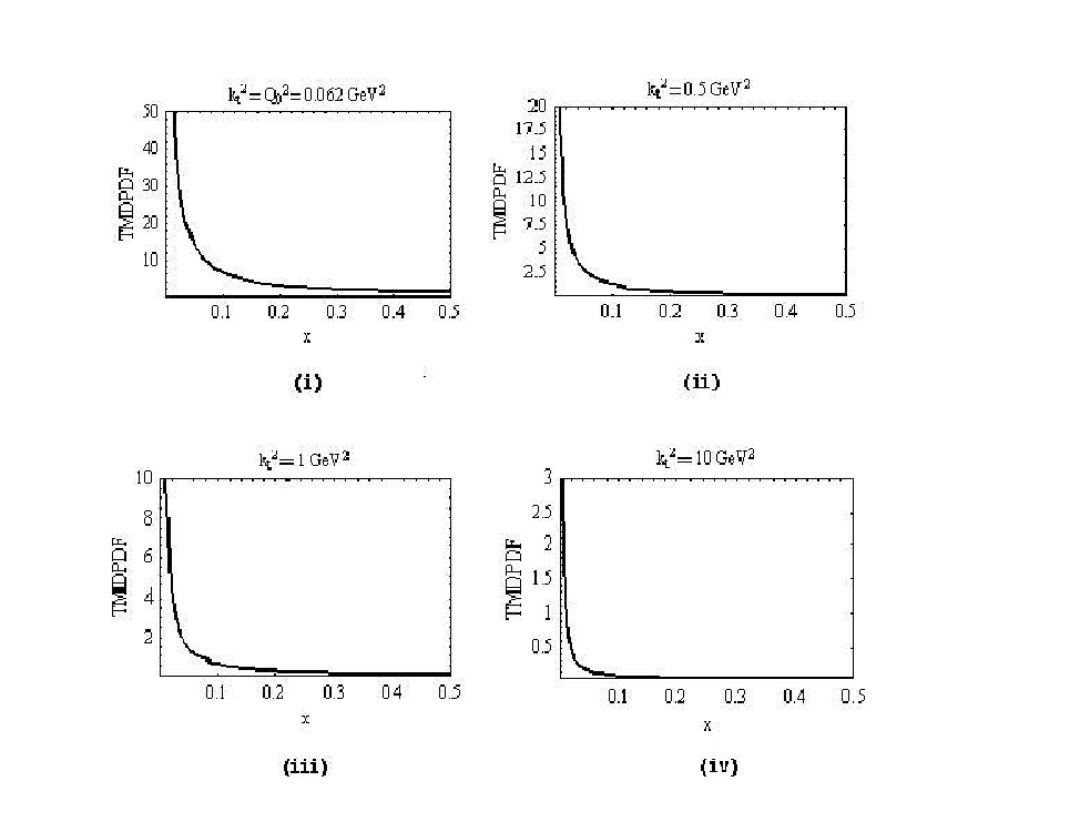
Using Eq (39) and taking $n_{f}=4$, $D_{0}^{i}\approx 0.085$ (taking $D_{0}=\Sigma_{i}D_{0}^{i}=n_{f}D_{0}^{i}$), $f_{i}(x,k_{t}^{2})$ is given by Eq (5), viz.

$$f_{i}(x,k_{t}^{2})=e^{D_{0}^{i}}\left(\frac{1}{x}\right)^{D_{2}+D_{1}\ln\left(1+\frac{k_{t}^{2}}{Q_{0}^{2}}\right)\left(1+\frac{k_{t}^{2}}{Q_{0}{2}}\right)^{D_{3}}}$$

(41)

In Figure 1, $f_{i}(x,k_{t}^{2})$ vs $k_{t}^{2}$ is shown for representative values of $\mathrm{(i)}\;x=10^{-4}\mathrm{(ii)}\;x=10^{-3}\mathrm{(iii)}\;x=10^{-2}$ and $\mathrm{(iv)}\;x=0.1$.

Similarly, $f_{i}(x,k_{t}^{2})$ vs x is shown in Figure 2 for representative values of $\mathrm{(i)}\;k_{t}^{2}=Q_{0}^{2}=0.062\;\mathrm{GeV}^{2}\mathrm{(ii)}\;k_{t}^{2}=0.5\;\mathrm{GeV}^{2}\mathrm{(iii)}\;k_{t}^{2}=1\;\mathrm{GeV}^{2}$ and $\mathrm{(iv)}\;k_{t}^{2}=10\;\mathrm{GeV}^{2}$.

References

- [1] I M Dremin, Mod. Phys. Lett. A3, 1333 (1988)
- [2] R Lipa and B Buschbeck, Phys. Lett. B223, 465 (1989)
- [3] W Florkowski and R C Hwa, Phys. Rev. D43, 1548 (1991)
- [4] James D Bjorken, SLAC-PUB-6477 (1994); arXiv:hep-ph/9610516
- [5] S N Banerjee, A Bhattacharya, B Chakraborty and S Banerjee, Int. J. Mod. Phys. A15, 2053 (2000); ibid. A16, 4939 (2001); ibid. A17, 4939 (2002)
- [6] I M Dremin and B B Levtchenko, Phys. Lett. B292, 155 (1992)
- [7] T Lastovicka, Euro. Phys. J. C24, 529 (2002); arXiv:hep-ph/0203260
- [8] T Lastovicka, Ph. D. Thesis, DESY Thesis 2004-016 (Humboldt University, Berlin, 2003)
- [9] D K Choudhury and Rupjyoti Gogoi; arXiv:hep-ph/0310260
- [10] D K Choudhury and Rupjyoti Gogoi; arXiv:hep-ph/0503047
- [11] Akbari Jahan and D K Choudhury; arXiv:1102.0069[hep-ph]
- [12] L Frankfurt, M Strikman and C Weiss, Ann. Rev. Nucl. Part. Sci. 55, 403 (2005); arXiv:hep-ph/0507286
- [13] V Rebyakova, M Strikman and M Zhalov, Phys. Rev. D81, 031501 (2010); arXiv:0911.5169 [hep-ph]
- [14] David d’Enterria and the CMS Collaboration, J. Phys. G: Nucl. Part. Phys. 34, S709 (2007)
- [15] V N Gribov and L Lipatov, Sov. J. Nucl. Phys. 15, 438 (1972); 15, 675 (1972)
- [16] Y L Dokshitzer, Sov. Phys. JETP 46, 641 (1977)
- [17] G Altarelli and G Parisi, Nucl. Phys. B126, 298 (1977)
- [18] C Aidala, S Liuti and C Riedl, arXiv:1007.4563 [hep-ph]
- [19] M A Kimber, J Kwiecinski, A D Martin and A M Stasto, Phys. Rev. D62, 094006 (2000); arXiv:hep-ph/0006184
- [20] M A Kimber, A D Martin and M G Ryskin, Phys. Rev. D63, 114027 (2001); arXiv:hep-ph/0101348
- [21] G Gustafson; arXiv:hep-ph/0312313
- [22] R G Roberts, The Structure of Proton (Cambridge University Press, Cambridge) p30 (1990)
- [23] F J Yudurain, Theory of Quark and Gluon Interactions (Springer Verlag, Berlin) p129 (1992)
- [24] C Pascaud and F Zomer, preprint DESY, 96-266 (1996)
- [25] M Froissart, Phys. Rev. 123, 1053 (1961)
- [26] A Martin, Scattering Theory: Unitarity, Analyticity and Crossing, Lecture Notes in Physics, Springer-Verlag, Berlin-Heidelberg-New York (1969)
- [27] M M Block, Edmond L Berger and Chung-I Tan, Phys. Rev. Lett. 97, 252003 (2006); arXiv:hep-ph/0610296
- [28] Edmond L Berger, M M Block and Chung-I Tan, Phys. Rev. Lett. 98, 242001 (2007); arXiv:hep-ph/0703003
- [29] F Carvalho, F O Duraes, V P Goncalves and F S Navara, arXiv:0705.1842 [hep-ph]
- [30] E A Kuraev, L N Lipatov and V S Fadin, Sov. Phys. JTEP 45, 199 (1977)
- [31] Ya. Ya. Balitskii and L N Lipatov, Sov. J. Nucl. Phys. 28, 822 (1978)
- [32] L N Lipatov, Sov. Phys. JTEP 63, 904 (1986)
- [33] L N Lipatov, Perturbative QCD, Edited by A H Mueller (World Scientific, Singapore, 1989)
- [34] V N Gribov, Sov. Phys. JETP 30, 709 (1970)
- [35] E Gotsman, E M Levin and U Maor, Eur. Phys. J. C5, 303 (1998); arXiv:hep-ph/9708275
- [36] M Ciafaloni, Nucl. Phys. B296, 49 (1988)
- [37] S Catani, F Fiorani and G Marchesini, Phys. Lett. B234, 339 (1990); Nucl. Phys. B336, 18 (1990)
- [38] I O Cherednikov and N G Stefanis, arXiv:0809.1315 [hep-ph]
- [39] N G Stefanis and I O Cherednikov, arXiv:0910.3108 [hep-ph]
- [40] Bernhard Musch, arXiv:0907.2381 [hep-lat]
- [41] B B Mandelbrot, Fractal Geometry of Nature, W H Freman, New York (1982)
- [42] T K Gaisser and F Halzen, Phys. Rev. Lett. 54, 1754 (1985)
- [43] M M Block and F Halzen, Phys. Rev. D70, 091901 (2004); arXiv:hep-ph/0405174
- [44] M M Block and F Halzen, Phys. Rev. D72, 036006 (2005); arXiv:hep-ph/0506031
- [45] ZEUS Collaboration: M Derrick et al, Z. Phys. C65, 379 (1995)
- [46] H1 Collaboration: T Ahmed et al, Nucl. Phys. B439, 471 (1995)
- [47] Hsiang-nan Li, Phys. Lett. B429, 121 (1998); arXiv:hep-ph/9709236
- [48] S Meiner, A Metz and K Goeke, Phys. Rev. D76, 034002 (2007)
- [49] D K Choudhury and Rupjyoti Gogoi, Indian J. Phys. 80, 659 (2006); arXiv:hep-ph/0503047
- [50] Francis C Moon, Chaotic and Fractal Dynamics: An Introduction for Applied Scientists and Engineers, John Wiley, New York, p364 (1992)
- [51] D K Choudhury and P K Sahariah, Pramana J. Phys. 60, 563 (2003)
- [52] A Donnachie and P V Landshoff, Z. Phys. C61, 139 (1994); arXiv:hep-ph/9305319
- [53] A Donnachie and P V Landshoff, Phys. Lett. B437, 408 (1998); arXiv:hep-ph/9806344
- [54] J R Cudell, A Donnachie and P V Landshoff, Phys. Lett. B448, 281 (1999);arXiv:hep-ph/9901222
- [55] H Kröger, Phys. Rep. 323, 81 (2000)